High-resolution land surface modelling over Africa: the role of uncertain soil properties in combination with forcing temporal resolution

Land surface modelling runs conducted with the Community Land Model version 5.0 (CLM5) over Africa at 3 km resolution were carried out, and we assessed the impact of different sources of soil information and different upscaling strategies for the soil information, in combination with different atmospheric forcings and different temporal resolutions of those atmospheric forcings. FAO and SoilGrids250m soil information was used. SoilGrids information at 250 m resolution was upscaled to the 3 km grid scale by three different methods: (i) random selection of one of the small SoilGrids250m grid cells contained in the model grid cell, (ii) arithmetic averaging of SoilGrids soil texture values, and (iii) selection of the dominant soil texture. These different soil model inputs were combined with different atmospheric forcing model inputs, which provide inputs at different temporal resolutions: CRUNCEPv7 (6-hourly input resolution), GSWPv3 (3-hourly), and WFDE5 (hourly). We found that varying the atmospheric forcing influenced the states and fluxes simulated by CLM5 much more than changing the soil information. Varying the source of soil texture information (FAO or SoilGrids250m) influences model water balance outputs more than the upscaling methodology of the soil texture maps. However, for a high temporal resolution of atmospheric forcings (WFDE5), the different soil texture upscaling methods result in considerable differences in simulated evapotranspiration (ET), surface runoff, and subsurface runoff at the local and regional scales, which is related to the higher-temporal-resolution representation of rainfall intensity in the model. The upscaling methodology of fine-scale soil texture information influences land surface model simulation results but only when clearly in combination with high-temporal-resolution atmospheric forcings.

1 Introduction

Understanding the intricate dynamics of land surface models (LSMs) over Africa involves a detailed examination of soil properties, which are indispensable yet steeped with uncertainty. The heterogeneity and complexity of soil properties (Vågen et al., 2016; Hengl et al., 2021) influence LSM simulations (Li et al., 2022), yet they often remain inadequately described within LSMs (Xu et al., 2023) due to limited data availability as a result of spatially insufficient measurements (Dube et al., 2023). This inadequacy is further exacerbated in LSMs by the need to represent the point-scale measurements at a coarse spatial resolution for field-, regional-, or continental-scale studies. Consequently, upscaling of soil information becomes a critical undertaking, aiming to bridge the gap between the fine-scale variability of soil properties and the broader scale at which LSMs usually operate (Van Looy et al., 2017; Montzka et al., 2017).

The quality of input datasets, like atmospheric forcings, soil physical properties, or land surface parameters, was found to greatly impact land surface modelling. Vahmani and Hogue (2014) compared remotely sensed green vegetation fraction (GVF) and impervious surface area (ISA) with the default look-up-table-derived values of the same parameters. The authors found that, using the remotely sensed parameters, the model was able to replicate the observed ET. This feat was attributed to capturing all year-round irrigation by means of the remotely sensed data in the domain of interest. This highlights the importance of the source of the datasets input into LSMs. The sensitivity of land surface models to atmospheric forcings as exemplified by Traore et al. (2014) over Africa was analysed with two atmospheric forcing datasets: Watch Forcing Data Era Interim (WFDEI) and Watch Forcing Data (WFD). These two reanalysis datasets were generated using the same methodologies but with a slight difference in their source datasets (Weedon et al., 2014). The results showed that, although there is a poor performance in terms of ET in Central African forests, WFDEI was closer to eddy covariance measurements than WFD, with correlations between 0.25 and 0.40. Lovat et al. (2019) used the ISBA-TOP coupled system (Bouilloud et al., 2010) over locations in the Mediterranean region at varying resolutions to assess river discharge and spatial runoff. It was noted that soil texture influences river discharge and runoff more than land cover does. Tafasca et al. (2020) used the land surface model ORCHIDEE and various global soil texture maps and noted that SoilGrids1km, upscaled to 0.5° by selecting the dominant soil type, generated similar water budgets as the 5 arcmin FAO Soil Map of The World (Reynolds et al., 2000) and the 1° resolution Global Soil Types map of Zobler (1986). The authors did, however, indicate that the weak model sensitivity to the soil texture variation could have been caused by the coarse spatial resolution of 0.5° at which soil texture was discretized in the ORCHIDEE model.

These existing gaps in data and the critical impact of their uncertainties on LSM performance highlight the need for detailed studies. Studying how varying resolutions of soil and atmospheric data affect high-resolution LSM outputs across diverse African ecosystems could help in refining model parameters and improving prediction accuracy. Furthermore, exploring new methods for effectively upscaling fine-scale soil measurements to broader applications in LSMs could provide insights into more robust upscaling strategies.

In this work, we are concerned with understanding the role of high-resolution soil texture input (at 3 km horizontal spatial resolution) and its upscaling in the Community Land Model version 5.0 (Lawrence et al., 2019) (hereafter, CLM5) simulations over the entire African continent. This study investigates the impact of uncertainty in soil input variables and the upscaling method of soil texture information at different spatial scales (from local to continental) and also in combination with different temporal resolutions of atmospheric forcings. The aim is not to compare simulations with measurements but rather to detect model-internal sensitivities to (the upscaling of) soil texture information.

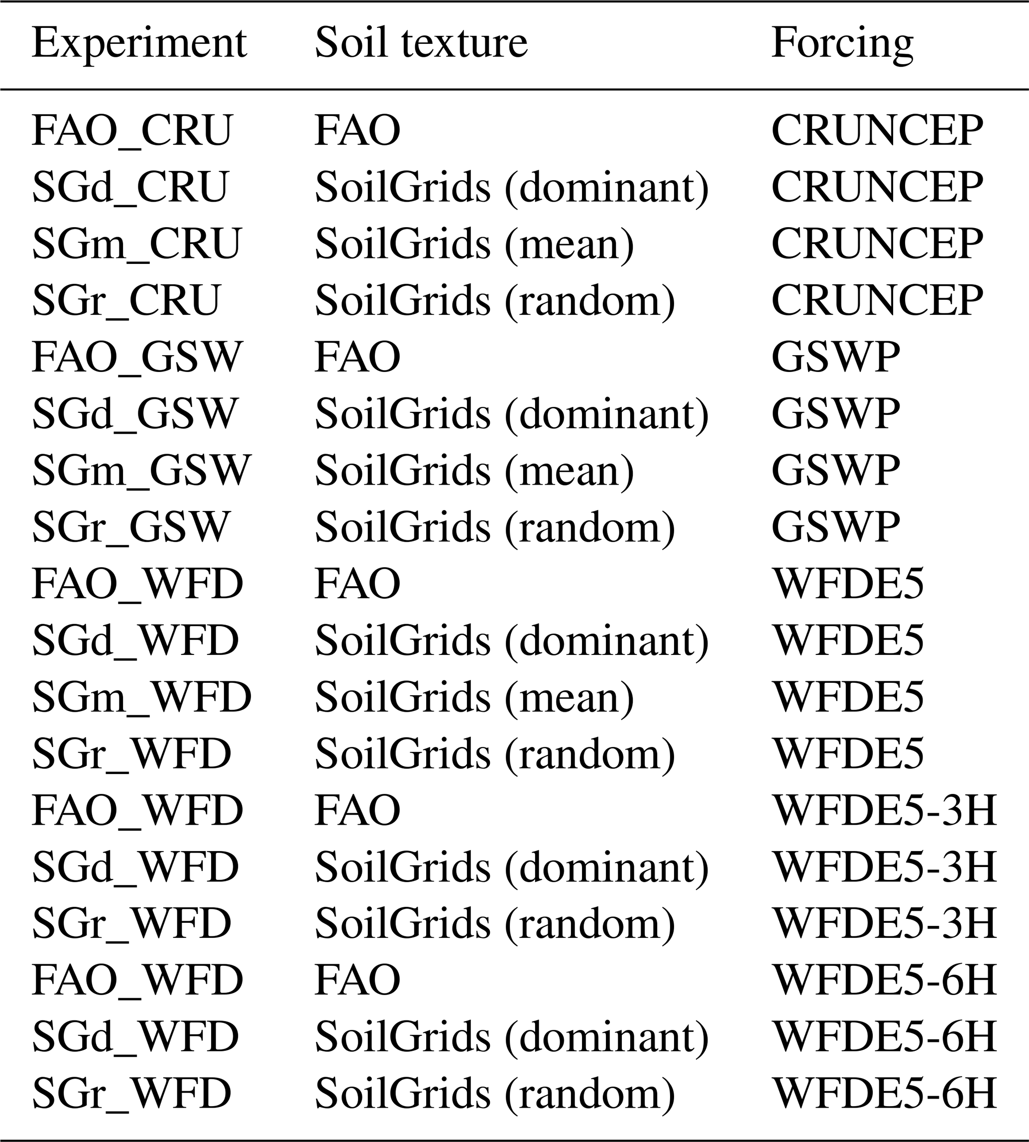
Twelve simulations combining four different soil texture inputs (FAO (Global Soil Data Task, 2014) and three differently upscaled SoilGrids maps (Hengl et al., 2017) and three different meteorological forcings were carried out, and results are analysed in this work at the continental, regional, and point scale. We also compared our outputs with an external dataset, GLDAS-2.1 (Beaudoing and Rodell, 2020), to assess the performance of the different upscaling methods. The novelty of this work lies in the detection of the impact of uncertainty in the (upscaling of) soil texture information, especially in combination with different temporal resolutions of atmospheric forcings. The impact of uncertainties of atmospheric forcings on land surface model simulations over Africa has been studied (Boone et al., 2009; Iyakaremye et al., 2021), but its interaction with the uncertainties in soil information has not been studied over Africa at a high spatial resolution.

This research therefore seeks to answer the following questions: (1) are simulation results of CLM5 sensitive to different soil texture inputs and the different upscaling methods applied to soil texture input? (2) What is the role of the temporal resolution of atmospheric forcings in combination with the different soil texture inputs?

2 Materials and methods

2.1 CLM5

CLM5 is a mechanistic land surface model which represents land surface heterogeneity differently from most other land surface models previously used over Africa in continental simulations (Traore et al., 2014; Ghent et al., 2010; Weber et al., 2009). While some of the models previously used over Africa had a single-layered sub-grid system popularly known as a mosaic system, CLM5 uses a multi-layered sub-grid hierarchy. This means that, in CLM5, each grid cell represents multiple land units consisting of vegetated, lake, urban, and glacier areas. Each land unit represents multiple columns which could have different soil profiles with autonomously evolving vertical profiles of soil moisture content and temperature, and each column has multiple patches of plant functional type (PFT) or crop functional type (CFT) (Lawrence et al., 2019). Among the numerous improvements in CLM5 compared to its predecessor are the inclusion of a spatially variable soil depth, the replacement of the Ball–Berry model with Medlyn stomatal conductance, and updated irrigation scheduling (Lawrence et al., 2019). Considering Africa's land surface heterogeneity, CLM5 has features of great interest for land surface modelling over Africa at a high spatial resolution.

CLM5 provides a framework for modelling the soil processes necessary for understanding terrestrial hydrology. This version of the model improves the representation of soil porosity and pore size distributions considering both mineral and organic components of the soil (Lawrence et al., 2019). Saturated hydraulic conductivity and soil matric potential are calculated using the method of Cosby et al. (1984) for mineral soils, with modifications to accommodate the effects of organic matter based on its depth and content. Detailed equations are comprehensively provided in Lawrence et al. (2019).

Furthermore, CLM5 employs the Brooks and Corey model (Brooks and Corey, 1964) to associate soil moisture content with water potential considering the variability in soil texture using organic and mineral soil fraction parameters.

$$\begin{array}{}\text{(1)}& B_i=\left(\mathrm{1}-f_{\left\{\mathrm{om},i\right\}}\right)\cdot B_{\left\{\min ,i\right\}}+f_{\left\{\mathrm{om},i\right\}}\cdot B_{\left\{\mathrm{om}\right\}}\end{array}$$

In the above, B_{om} covers organic matter, f_{om,i} represents organic matter fraction, and

$$\begin{array}{}\text{(2)}& B_{\left\{\min ,i\right\}}=\mathrm{2.91}+\mathrm{0.159}\cdot {\left(\mathit{\%}\left\{\mathrm{clay}\right\}\right)}_i\end{array}$$

is for mineral soil, where (%{clay}) is the percentage of clay in each grid cell at level i.

The full water balance equation now implies interactions between canopy, surface, soil, and aquifer water and ice storage, defining the model's detailed approach to hydrologic partitioning over varying temporal scales.

The water balance equation is represented by

$$\begin{array}{}\text{(3)}& \begin{array}{rl}\mathrm{\Delta }\mathrm{Sc},\mathrm{l}& +\mathrm{\Delta }\mathrm{Sc},\mathrm{sn}+\mathrm{\Delta }\mathrm{Ssfc}+\mathrm{\Delta }\mathrm{Ssn}\\ & +{\sum }_{i=\mathrm{1}}^{N_{\mathrm{levso}},i}\left(\mathit{\theta }{s}_{\mathrm{liq},i}+\mathit{\theta }{s}_{\mathrm{ice},i}\right)+\mathrm{\Delta }\mathrm{Sacq}\\ & =(\mathrm{qrn}+\mathrm{qsn}-\mathrm{Ev}-\mathrm{Eg}-\mathrm{qover}\\ & -\mathrm{qsfcwat}-\mathrm{qdr}-\mathrm{qrgl}-\mathrm{qsnsfc})\mathrm{\Delta }t,\end{array}\end{array}$$

where ΔScl represents changes in canopy water, ΔScsn represents changes in canopy snow, ΔSsfc represents changes in surface water, ΔSsn represents changes in surface snow, and ΔSacq represents changes in water stored in the aquifer. θs_liq,i represents changes in soil water, and θs_ice,i represents changes in soil ice at each soil level i. N_levso,i refers to the number of soil levels. On the right-hand side of the equation, qrn represents rainfall, qsn represents snowfall, Ev represents transpiration, and Eg represents evaporation, while qover refers to surface runoff, qsfcwat refers to runoff from surface water storage, qdr refers to drainage, qrgl refers to glacier and lake runoff, and qsnsfc refers to snow-capped surface runoff. Precipitation (qrn + qsn) is intercepted by the canopy, which is controlled by leaf area index. The moisture input reaching the surface after evaporative losses from both the vegetation and the surface (Ev, Eg) is then divided between surface runoff, surface water storage, and infiltration. The unit for fluxes is kg m⁻² s⁻¹, while storage variables are quantified in kg m⁻², and Δt is in mm s⁻¹. For a detailed description of the mathematical formulations and their applications within CLM5, readers are referred to Lawrence et al. (2019), where these processes are described in-depth.

Irrigation in CLM5 separates irrigated and rainfed crops by assigning them to separate soil columns. Irrigation is applied daily at 06:00 (simulation local time per grid cell) based on the difference between soil moisture content and target soil moisture while also taking the crop leaf area index into account. Irrigation decisions are guided by datasets detailing areas equipped for irrigation according to Portmann et al. (2010). To constrain CLM5 irrigation, irrigation water is sourced from river storage, with provisions for supplements from ocean reserves. Alternatively, in severe cases of water scarcity, irrigation demand is dynamically adjusted to conserve river water levels. The applied irrigation in CLM5 is hard-coded to bypass canopy interception, meaning it is added directly to the ground surface. More details can be found in Lawrence et al. (2019).

2.2 Soil texture information

Soil hydraulic and thermal properties are critical for flux and state calculations in LSMs (Zhao et al., 2018). These values are generally obtained from soil texture information through pedotransfer functions, which is also the case for CLM5. Two different soil texture datasets, the IGBP-DIS soil dataset and the SoilGrids250m dataset, were used as input for CLM5 simulations over Africa. The IGBP-DIS soil dataset was generated using the linkage method, which is characterized by lack of intra-polygonal variation. This soil texture dataset constitutes the default soil texture information available in CLM5. The soil texture dataset, which is at approximately 8 km resolution, provides information for the top 10 CLM5 soil layers at 0.0175, 0.0451, 0.0906, 0.1656, 0.2892, 0.493, 0.829, 1.3829, 2.2962, and 3.4332 m depth.

ISRIC's SoilGrids250m (Hengl et al., 2017) was produced by machine learning, and it is the successor of the SoilGrids1km product (Hengl et al., 2014). SoilGrids250m has a spatial resolution of 250 m and is therefore considered because of its potential to better represent local-scale soil processes as a result of the higher spatial resolution. When evaluated with soil profiles from WoSIS (World Soil Information Service), SoilGrids250m has a higher accuracy than FAO, with an RMSE of 18.6 % versus 26.3 % for the sand fraction at 0–30 cm depth and 12.5 % versus 15.4 % for clay fractions at this depth (Dai et al., 2019).

Improvements in SoilGids250m compared to its earlier version, SoilGrids1km, include, for example, further soil information for deserts and arid areas such as the Sahara Desert, covering about 30 % of Africa's land mass (Tucker and Nicholson, 1999). About 150 000 soil profiles were obtained globally across all continents from both actual observations and pseudo-observations. Actual observations were from in situ and remote sensing measurements and values reported by national classification systems. Pseudo-observations came from expert assessment of both restricted areas and places with extreme climate conditions like deserts, glaciers, mountaintops, tropical forests, and austere regions. SoilGrids250m provides global estimates for soil texture fractions, organic carbon, bulk density, cation exchange capacity, pH, and coarse fragments. Compared to SoilGrids1km, SoilGrids250m records a relative improvement of over 60 % in sand, silt, and clay contents, as explained by a 10-fold cross-validation exercise. The Soilgrids250m, unlike the IGBP-DIS, was provided at seven standard soil depths of 0, 0.05, 0.15, 0.30, 0.60, 1.00, and 2.00 m depth.

2.3 Upscaling of soil textural properties

Upscaling of soil hydraulic properties is needed when the model resolution is coarser than the resolution of the measurement-based product. SoilGrids250m soil texture information needs to be upscaled to the 3 km × 3 km resolution of the CLM5 model for Africa. One CLM5 grid cell therefore contains 144 SoilGrids250m grid cells. Three upscaling methods of soil texture information were compared in this work:

• i.

  The first method is simple averaging of the soil texture values for all the SoilGrids grid cells which are contained in a larger CLM grid cell (e.g. Kochendorfer and Ramírez, 2010). Since information on both clay and sand soil texture was provided as fractions per grid cell, a simple averaging of the fractions was performed.

• ii.

  The second method is selection of the dominant soil type (according to USDA soil classification) in a CLM grid cell and use of the soil texture values for that soil type for the complete CLM grid cell. This method was, for example, used in Tafasca et al. (2020). The dominant soil type is any soil type with the highest representation among the 144 SoilGrids grid cells.

• iii.

  Finally, we conduct random selection of a single SoilGrids cell and use the soil texture values for this grid cell for the complete 3 km × 3 km CLM model grid cell. This method, which is a novelty of this work, creates a chance for texture outliers to define the soil hydraulic parameters. This ensures that, over larger regions, the probability density function (PDF) of soil properties is better reproduced by the model than by selecting the dominant soil texture or average soil texture. It differs from other upscaling methods as it avoids spatial averaging or smoothing. Although it can introduce larger local biases in the soil hydraulic parameters and thus model output variables, it is not expected to induce systematic biases at larger scales as local biases for some grid cells will be cancelled out by biases at other grid cells. In addition, as soil texture is not averaged or smoothed before being processed through the non-linear simulation model, it is expected that model output variables, averaged over larger areas, are also unbiased. We also specified a random-number generator (RNG) seed, which makes the randomization reproducible in other machines.

2.4 Meteorological forcing datasets and evaluation dataset

In this work, the impact of three different meteorological forcing datasets with different temporal resolutions, in combination with the different soil texture input datasets, was investigated. We examined CRUNCEPv7 (Viovy, 2018), GSWP3 (Hyungjun, 2017), and WFDE5 (the bias-corrected ERA5 dataset using the WATer and global CHange (WATCH) Forcing Data methodology) (Cucchi et al., 2020). These three forcings have been selected because they possess all the atmospheric variables CLM5 requires and have similar spatial resolutions and, in particular, varying temporal resolutions of 6 h (CRUNCEP), 3 h (GSWP), and 1 h (WFDE5). The impact of the varying temporal resolutions was studied in combination with the different soil texture inputs. GSWPv3 and CRUNCEPv7 have already been used in the past in combination with CLM4, CLM4.5, and CLM5 (Bonan et al., 2019). WFDE5 has been tested at 13 globally spread FLUXNET2015 locations. Cucchi et al. (2020) showed that WFDE5 has smaller mean absolute errors and larger correlations of variables like precipitation, global radiation, specific humidity, air temperature, and wind speed with observations than the WFDEI (Watch Forcing Data ERA Interim) dataset, which was used in Traore et al. (2014) over Africa. For comparison and assessment of the different upscaling-method performances, the GLDAS-2.1 dataset was used. The dataset has been used over Africa to train deep learning algorithms for modelling groundwater (Gaffoor et al., 2022), calculating drought recovery time (Hao et al., 2022), and assessing the spatio-temporal patterns of drought in East Africa (Liu et al., 2022). Our choice of the GLDAS-2.1 dataset is motivated by the fact that it provides soil moisture information from 0 to 200 cm.

• i.

  CRUNCEPv7. CRUNCEPv7 dataset is a combination of CRU (Climate Research unit Time Series) 3.24 (Harris, 2013) and National Centre for Environmental Protection (NCEP) reanalysis (Kalnay et al., 1996). The data are available for the period between 1901 and 2016 with a horizontal resolution of 0.5° and 6 hourly temporal resolution. Precipitation, cloudiness, temperature, and relative humidity were taken from CRU while wind speed, pressure and long wave radiation were obtained from NCEP.

• ii.

  GWSP3. The Global Soil Wetness Project version 3 dataset is a 3-hourly atmospheric forcing product at 0.5° horizontal resolution. The data are available for the period between 1900 and 2014 and are based on NCEP's 20th-century reanalysis project (Compo et al., 2011). Though the 20th-century project dataset was published at 2° horizontal resolution, the GSWP version 3 dataset was downscaled to 0.5° horizontal resolution using a spectral-nudging technique (Yoshimura and Kanamitsu, 2008). Four out of seven variables, namely air temperature, precipitation, and longwave and shortwave radiation, were bias-corrected using the Climate Research Unit's CRU Tsv3.21 (Harris, 2013), the Global Precipitation Climatology Centre's GPCCv7 (Schneider et al., 2014), and surface radiation budget datasets (Lawrence et al., 2019). GSWP3 is the default forcing provided with the CLM5 model (Lawrence et al., 2019). Since both GSWP3 and CRUNCEPv7 datasets were provided for use in CLM by the developers, there was no additional processing needed to use these datasets in CLM5.

• iii.

  WFDE5. The WFDE5 dataset was created by using the WATer and global CHange (WATCH) Forcing Data methodology to process near-surface fifth-generation ECMWF (European Centre for Medium-Range Weather Forecasts) Reanalysis (ERA5) variables. WFDE5 was provided globally on a regular long–lat grid at 0.5°×0.5° spatial resolution at hourly time steps. It therefore has the highest temporal resolution of the atmospheric forcing datasets considered in this study. WFDE5 correlates better with FLUXNET2015 datasets at each site than WFDEI (Traore et al., 2014). Another advantage WFDE5 has over the higher-spatial-resolution ERA5 dataset is that the monthly precipitation totals were bias-corrected using precipitation data from the Climate Research Unit Time Series (CRU TS) and the Global Precipitation Climatology Centre (GPCC). This is important as precipitation has a large impact on LSM simulations compared to other meteorological forcings (Bucchignani et al., 2016) over Africa.

• iv.

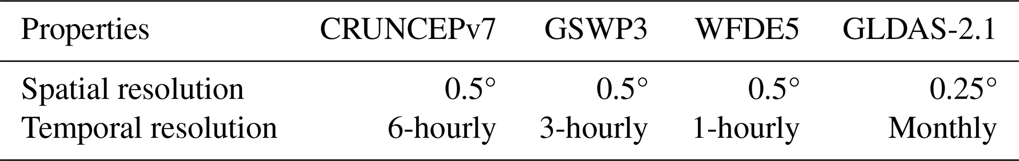
  GLDAS-2.1. The GLDAS-2.1 dataset was used for verification purposes in this work. The Global Land Data Assimilation System was originally developed to absorb satellite- and ground-based observational data products using advanced land surface modelling and data assimilation techniques in order to generate fields of land surface states and fluxes (Rodell et al., 2004). The GLDAS-2.1 dataset, which was reprocessed in January 2020, delivers monthly 0.25° data produced by temporal averaging of 3-hourly simulations using the Noah-MP land surface model 3.6 (LIS, version 7). The GLDAS-2.1 simulations were driven by NOAA/GDAS atmospheric fields, GPCP V1.3 precipitation data, and AGRMET radiation variables from March 2001 onward. Table 1 summarizes the details regarding the different meteorological forcing and evaluation datasets used in this work.

Table 1 Main properties of the reanalysis datasets CRUNCEPv7, GSWPv3, WFDE5, and GLDAS-2.1 used in this work.

2.5 Model setup and analysis

In this work, CLM5 was run in land-only mode; i.e. instead of coupling CLM5 with an atmospheric model, atmospheric reanalysis datasets are used as external forcings of the land surface model. Atmospheric input into CLM5 includes precipitation, incoming shortwave radiation, air temperature, surface air pressure, specific humidity, wind speed, and incoming longwave radiation. These are available every 6 h for CRUNCEP, every 3 h for GSWP, and hourly for WFDE5. However, since the model time step is 30 min, precipitation is divided equally over the different model time steps. For air temperature, surface air pressure, specific humidity, and wind speed, all values are interpolated to model time steps using the nearest-neighbour algorithm. For solar radiation, the cosine of the solar zenith angle is used to ensure a smoother diurnal cycle while preserving the total radiation from the atmospheric input data.

Sixteen plant functional types were activated alongside transient CO₂ and aerosol deposition rates. All 12 model simulations (Table 2) apply monthly leaf area index (LAI) as observed from satellite phenology. A spatially varying soil thickness dataset (Pelletier et al., 2016), with values ranging from 0.4 to 8.5 m, was also applied. The land cover description is based on 1 km resolution Moderate Resolution Imaging Spectroradiometer (MODIS) products. Land cover type is from MCD12Q1 version 5, which provides annual land cover intervals between 2000 and 2015.

Twelve simulations (three atmospheric forcings combined with four soil texture maps) were performed over the CORDEX Africa domain, which covers 45.76° S to 42.24° N latitude and −24.64° W to 60.28° E longitude (results over African continent only). The horizontal resolution for all model simulations was approximately 0.027°, i.e. about 3 km. This discretization results in 10 033 920 grid cells. The simulation period was from 1 January 2011 to 31 December 2014, and the results for the first 2 years were discarded (spin-up period). Earlier works over the southern African region, including Crétat et al. (2012), Ratna et al. (2014), and Zhang et al. (2023), have employed spin-up times of 6 months or less using different land surface models, while Zheng et al. (2017) employed 1 year for spin-up with a predecessor of CLM5 over the Tibetan Plateau. We compared the simulated water balance components in this work with water balance components (evapotranspiration, surface runoff, and soil water content) from a fresh simulation which had 11 years of spin-up time, and the results do not alter the initial conclusion of this study (Figs. S54–56 in the Supplement). Moreover, we evaluated the adequacy of the reference period employed in this study. The continental annual average of the deepest soil moisture layer was calculated, a trend line was fixed, and the statistical significance was calculated to determine whether the slope of the trend differed significantly from zero. The resulting p value of 0.353 indicated that the trend in soil moisture over the 3-year period was not statistically significant based on a 95 % confidence interval (Fig. S57 in the Supplement), suggesting that extending the study period will not alter the current outcome.

Although the model time step size was 30 min, most results are presented as monthly sums (at regional and local scales). For continental-scale results, annual mean of evapotranspiration (ET), surface runoff, and subsurface runoff were computed, along with the seasonal mean of the weighted average of the top 2 m soil moisture content. The weights for calculating the weighted average of soil moisture content were defined according to the thickness of each soil layer in CLM5.

To further substantiate the role of soil texture input into CLM5, a new set of simulations was conducted. To ensure comparability with CRUNCEP (6-hourly) and GSWP (3-hourly), the hourly WFDE5 forcings were aggregated to 6 and 3 h, respectively. The model was then run with the soil texture information. This was conducted to identify discrepancies between the simulation outcomes of WFDE5 at hourly and 3 and 6 h temporal resolutions. Furthermore, a comparison was made with the results obtained by CRUNCEP and GSWP. The results were also analysed at the monthly level in addition to the regional and local time series.

A metric termed “average margin” was introduced to quantify the impact of the temporal resolution of atmospheric forcings in combination with soil texture map variation. The four soil texture maps were considered, each providing a unique output at every time step within the time series. The average margin for a simulated variable for a certain atmospheric forcing and/or soil texture map combination at a given time step is denoted by M₁(t), M₂(t), M₃(t), and M₄(t). The difference in terms of the maximum and minimum simulated value for the variable between the soil texture maps at a given time step is then computed as

$$\begin{array}{}\text{(4)}& \begin{array}{rl}D\left(t\right)& =max\left(M_{\mathrm{1}}\left(t\right),M_{\mathrm{2}}\left(t\right),M_{\mathrm{3}}\left(t\right),M_{\mathrm{4}}\left(t\right)\right)\\ & -min\left(M_{\mathrm{1}}\left(t\right),M_{\mathrm{2}}\left(t\right),M_{\mathrm{3}}\left(t\right),M_{\mathrm{4}}\left(t\right)\right),\end{array}\end{array}$$

and the average margin is given by

$$\begin{array}{}\text{(5)}& A={\displaystyle \frac{\mathrm{1}}{T}}{\sum }_{t=\mathrm{1}}^{T}D\left(t\right),\end{array}$$

where T represents the total number of time steps in the time series, and t denotes the time step.

A one-way analysis of variance (ANOVA) was conducted to ascertain whether the outputs of the four soil maps for each atmospheric forcing group exhibited significant variation. Firstly, the mean of the four soil map outputs was calculated, and the deviation of each map's output from the mean was obtained. The resulting deviations were subsequently expressed as percentages relative to the mean output, thus providing a normalized measure of the deviation for each soil map, which could then be compared with results for other atmospheric forcings. The data were subsequently transformed into a long format suitable for ANOVA, in which the percentage deviations for each soil map were compared. The dependent variables were the obtained percentage deviations, while the independent variables were the categorical variable defining the compared groups (FAO, dominant, mean, and random). Subsequently, an analysis of variance (ANOVA) was conducted to ascertain whether there were statistically significant discrepancies between the models' percentage deviations. The results of the ANOVA analysis yielded a p-value statistic, which was used to determine the significance of the observed variations in soil texture map outputs at the 95 % confidence interval. For further details on the ANOVA framework, we direct the reader to the works of Fisher (1925) and Brandt (2014).

Finally, we compared the different soil texture map outcomes with the GLDAS-2.1 dataset as a benchmark to compare CLM5 model outputs to an established external dataset. We compared ET, surface runoff and soil moisture content using the Pearson correlation (Pearson and Henrici, 1997) to measure the strength of the relationship between the datasets and the root mean square error (RMSE). More details about the RMSE and its proper use are described by Hodson (2022). For the reference study period, for every grid cell and all time steps, the calculated water balance components were compared with the ones from the GLDAS-2.1 dataset. This comparison was performed on a grid-cell-by-grid-cell basis, resulting in a complete continental assessment of the water balance components.

Table 2 Summary of CLM5 experiments in this study combing different soil texture input information and atmospheric forcings.

2.6 Definition of regions

Iturbide et al. (2020) updated the IPCC climate reference regions for subcontinental analysis based on, amongst others, the coherence of climate variables. The new reference regions for Africa include the Mediterranean, Sahara, West Africa, northeastern Africa, Central Africa, central East Africa, southwestern Africa, and southeastern Africa. Here, we combined southeastern Africa and Madagascar into one region. Figure S1 shows the African sub-regions. The eight regions are used as a basis to calculate region-specific water balance components.

3 Results and discussion

3.1 Comparison of simulated water balance components with GLDAS-2.1 datasets

To assess the agreement between the CLM5-simulated water balance components and a reference dataset, a comparison was conducted with the outputs of GLDAS-2.1. We acknowledge that, while the GLDAS-2.1 serves as a benchmark for comparison, the extent to which it accurately represents actual conditions remains uncertain.

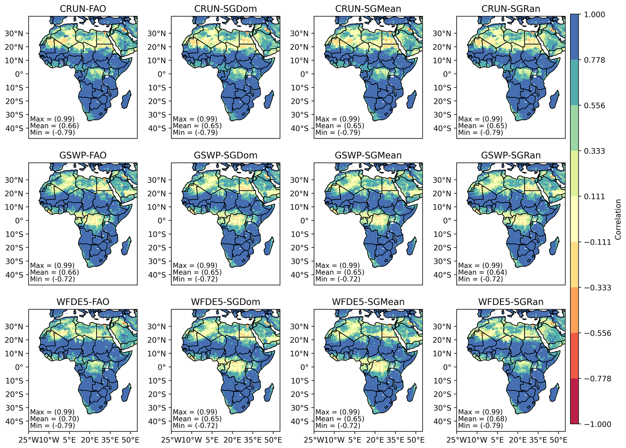
Figure 1 Temporal correlation maps of simulated evapotranspiration compared with the Global Land Data Assimilation System (GLDAS-2.1) dataset over Africa for three different atmospheric forcing datasets (CRUN, GSWP, and WFDE5) and four soil texture maps (FAO and SoilGrids (dominant – SGDom; mean – SGMean; and random – SGRan)). Top row: correlation maps for the CRUNCEP dataset using the FAO, SGDom, SGMean, and SGRan soil texture maps. Middle row: correlation maps for the GSWP dataset using the same four soil texture maps. Bottom row: correlation maps for the WFDE5 dataset using similar maps.

3.1.1 Evapotranspiration

The correlation of CLM5-simulated ET with GLDAS (Fig. 1) shows a clear spatial gradient across Africa. Strong positive correlations above 0.75, as referenced in hydrology studies over Africa (Scanlon et al., 2022; Larbi et al., 2020), are mainly seen in the equatorial region and in parts of East Africa, southern Africa, and Madagascar, indicating acceptable model performance in these regions. Northern Africa, some parts of Central Africa, and the cape of South Africa tend to show moderate to weak positive correlations, with some areas having negative correlations (down to around −0.79). The mean correlation values hover around 0.64–0.70, reflecting relatively moderate agreement with GLDAS across the continent. The RMSE for ET (Fig. S50) displays a concentration of lower errors in the moisture-deficient northern and southern parts of Africa, while the moisture-richer central and eastern regions show higher RMSE values. This suggests that, while CLM5-simulated ET corresponds well with GLDAS in the equatorial zones, there is higher variability and model uncertainty in the arid and semi-arid regions. It is important to note, however, that RMSE scores are magnitude dependent as they increase or decrease with the magnitude of evaluated variables.

3.1.2 Surface runoff

Surface runoff correlations (Fig. 2) over Africa exhibit wide variability, with very high positive correlations (up to 1.0) in savannah regions of West Africa, including parts of Namibia, Zambia, and Mozambique. There are, however, areas with low to strongly negative correlations, particularly in Mauritania, Mali, Algeria, Libya, Egypt, and Sudan, where correlation values are as low as −1.0. This high variability results in an average continental correlation of 0.50–0.58. The RMSE for surface runoff over Africa (Fig. S52) shows minimal errors in water-scarce northern and southwestern Africa, with the highest RMSE values ranging from 0 to 11 mm per month. Central Africa and western African regions show relatively higher RMSE values. The high RMSE values suggest substantial discrepancies in surface runoff simulation between CLM5 and GLDAS, especially in equatorial areas.

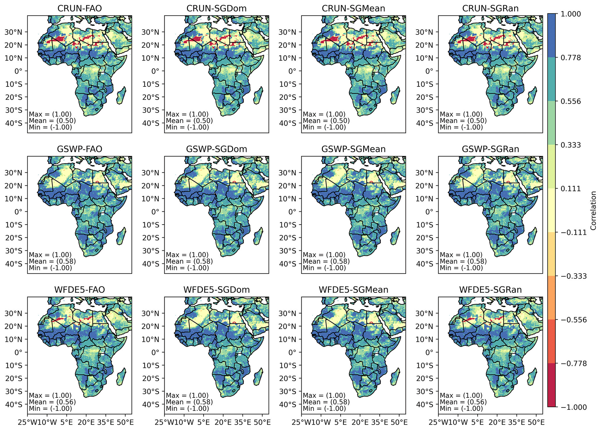
Figure 2 Temporal correlation maps of simulated surface runoff compared with the Global Land Data Assimilation System (GLDAS-2.1) dataset over Africa for three different atmospheric forcing datasets (CRUN, GSWP, and WFDE5) and four soil texture maps (FAO, SGDom, SGMean, and SGRan). Top row: correlation maps for the CRUNCEP dataset using the FAO, SGDom, SGMean, and SGRan soil texture maps. Middle row: correlation maps for the GSWP dataset using the same four soil texture maps. Bottom row: correlation maps for the WFDE5 dataset using similar maps.

3.1.3 Soil moisture

Soil moisture correlations with GLDAS (Fig. 3) show a slightly different spatial pattern compared to ET. The highest correlations (strong positive) are generally observed above the Equator, in the top fringes of southern Africa, and in northern Madagascar. However, strong negative correlations are found in parts of the Sahara, specifically Mauritania, Mali, Algeria, Egypt, and Sudan, where certain grid cells exhibit correlations as low as −0.79. Overall, the average correlations for soil moisture are lower than for ET, with a range of 0.56–0.67, indicating less correlation across the continent compared to ET. The RMSE map for soil moisture (Fig. S51) exhibits average values ranging between 0.05–0.06 cm³ cm⁻³. There is slightly higher RMSE in parts of Central Africa specifically, in the Democratic Republic of Congo, where errors peak around 0.26–0.27 cm³ cm⁻³. This RMSE pattern suggests that the CLM5-simulated soil moisture maintains a relatively stable agreement with GLDAS, having minimal extreme errors across the continent.

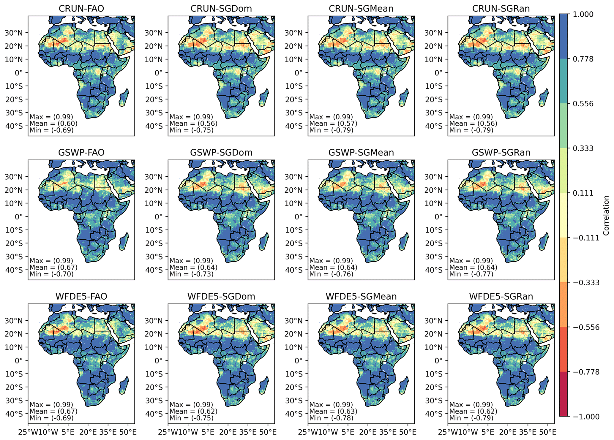
Figure 3 Pearson correlation maps of simulated soil water content compared with the Global Land Data Assimilation System (GLDAS-2.1) dataset over Africa for three different atmospheric forcing datasets (CRUN, GSWP, and WFDE5) and four soil texture maps (FAO, SGDom, SGMean, and SGRan). Top row: correlation maps for the CRUNCEP dataset using the FAO, SGDom, SGMean, and SGRan soil texture maps. Middle row: correlation maps for the GSWP dataset using the same four soil texture maps. Bottom row: correlation maps for the WFDE5 dataset using similar maps.

3.2 Continental simulated water balance components

3.2.1 Evapotranspiration

Figure 4 shows actual ET estimates over Africa for the different soil texture maps used in this study and the different atmospheric forcings. Continental average ET and local ET maxima were estimated for all 12 simulations for the reference period of 2013–2014.

The soil texture map has, in general, only a limited impact on simulated ET. For CRUNCEP-forced simulations, the yearly ET varies among the soil maps between 452.9 and 454.4 mm yr⁻¹, with the lowest ET for the FAO soil texture map and slightly higher ET for the SoilGrids texture maps. Also, for GSWP-forced simulations, we find the lowest simulated ET for the FAO soil texture map (438.7 mm yr⁻¹), while the highest simulated ET is only slightly higher (439.6 mm yr⁻¹). Simulated ET is highest for the SoilGrids soil map, which is randomly upscaled. Also, for the WFDE5 simulations, differences in simulated ET are very small and vary between 442.5 mm yr⁻¹ (FAO) and 443.5 mm yr⁻¹ (SoilGrids, randomly upscaled). These numbers also illustrate that the impact of variations in soil texture input is much smaller than that of variations in atmospheric forcings. While the four different soil texture maps result in maximum variations in average yearly ET over the African continent of only ∼ 1 mm for a given atmospheric forcing, the variations in atmospheric forcing result in maximum variations in average yearly ET over the African continent of around 14 mm yr⁻¹ for a given soil texture dataset. Specifically, the upscaling procedure of the soil texture information exhibits negligible effects on the mean annual estimates of evapotranspiration over Africa. Also, the maximum simulated ET for a grid cell over Africa is hardly affected by the soil texture map input (< 1 mm yr⁻¹), with even smaller variations among soil texture maps than the continental average. On the other hand, variations in atmospheric forcings affect the local maximum simulated yearly ET more strongly, with variations among forcings of ∼ 36 mm yr⁻¹.

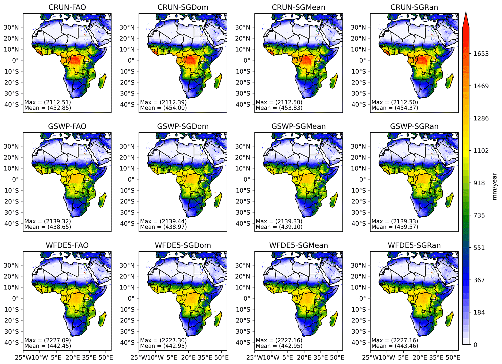
Figure 4 Spatial distribution of simulated mean annual evapotranspiration over Africa. Upper row: CRUNCEP-forced simulations with, from left to right, FAO, dominant, mean, and random upscaled soil texture map inputs. Middle row: like the upper row but for GSWP-forced simulations. Bottom row: like the upper row but for WFDE5-forced simulations.

3.2.2 Surface runoff

Also, the continental surface runoff is not strongly affected by variations in the soil texture map (Fig. 5). For all three atmospheric forcings, the average surface runoff over the African continent is almost the same for the four different soil texture maps, and differences in surface runoff are never larger than 0.3 mm yr⁻¹ for a given atmospheric forcing. When examining the influence of soil texture maps on surface runoff, it becomes evident that the disparities between the various SoilGrids maps, generated using different upscaling methods, are minimal. The maximum difference in continental averages of surface runoff between the SoilGrids soil texture maps with the highest and lowest values is only 0.01–0.02 mm yr⁻¹, depending on the atmospheric forcing. However, slightly larger differences are observed when comparing the FAO soil texture map with the SoilGrids texture maps, with a maximum variation of 0.20–0.26 mm yr⁻¹, again depending on the atmospheric forcing. These findings indicate that, while the upscaling process of soil texture maps does not substantially impact simulated surface runoff with CLM5, the source and type of soil texture maps employed do have a small, yet perceivable, influence on the results.

On the other hand, the atmospheric forcing shows a much larger impact on average surface runoff over Africa, with a value of approximately 94 mm yr⁻¹ for CRUNCEP (6-hourly temporal resolution), 114 mm yr⁻¹ for GSWP (3-hourly temporal resolution), and 122 mm yr⁻¹ for WFDE5 (hourly resolution). Spatial details can be found in Fig. 2. The substantial difference of 28 mm yr⁻¹ in average annual surface runoff between WFDE5 and CRUNCEP potentially contributes to higher ET estimates for CRUNCEP at 11 mm yr⁻¹. The increased surface runoff in the WFDE5-forced simulations reduces the availability of water for ET processes, especially after runoff events.

The differences in surface runoff could be related to the temporal resolution of the atmospheric forcings. A higher temporal resolution of the atmospheric forcings, as for WFDE5, will result in higher peaks of precipitation intensity, whereas a coarser temporal resolution of 6 h, like for CRUNCEP, will average out intensive precipitation over longer time periods, with fewer high peaks in precipitation intensity. As surface runoff is generated under conditions of (very) high precipitation intensity, it can be expected that the temporal resolution of the atmospheric forcings will affect the simulated amount of surface runoff.

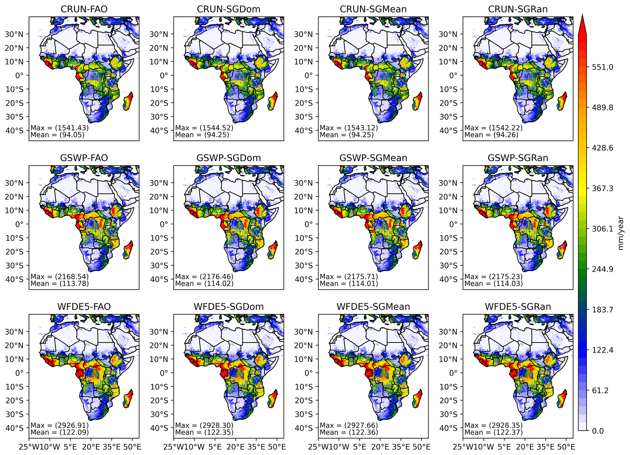
Figure 5 Spatial distribution of simulated mean annual surface runoff over Africa. Upper row: CRUNCEP-forced simulations with, from left to right, FAO, dominant, mean, and random upscaled soil texture map inputs. Middle row: similar to the upper row but for GSWP-forced simulations. Bottom row: similar to the upper row but for WFDE5-forced simulations.

3.2.3 Subsurface runoff

Simulated subsurface runoff across the African continent (Fig. 6) is, in general, low in most regions and across all simulation scenarios, typically below 250 mm yr⁻¹. The estimation of subsurface runoff is more influenced by soil texture variations and the upscaling of soil texture properties compared to ET and surface runoff simulations. The most substantial differences in simulated subsurface runoff among soil texture inputs are between the FAO soil map and the SoilGrids250m maps, while the disparities among the upscaled SoilGrids250m maps are smaller, especially with GSWP and CRUNCEP forcings. For CRUNCEP forcings, the difference between the maximum and minimum simulated subsurface runoff among the soil texture maps (averaged over Africa) is 11.3 mm yr⁻¹, whereas it is 2.1 mm yr⁻¹ among the upscaled SoilGrids maps. For GSWP, these differences are 11.6 and 2.4 mm yr⁻¹, respectively, while for WFDE5, they are 26.0 and 14.5 mm yr⁻¹, respectively. Notably, for WFDE5 (with 1-hourly forcings), the differences in simulated subsurface runoff among the different upscaled SoilGrids maps are considerably larger than for the other forcings. The variations in maximum subsurface runoff values among soil texture maps are more pronounced than for the mean subsurface runoff, particularly for CRUNCEP and WFDE5, where the differences among upscaled SoilGrids maps are also substantial.

On the other hand, the spatially averaged subsurface runoff over Africa showed considerable variations among atmospheric forcings: 17–29 mm yr⁻¹ for CRUNCEP, between 36 and 48 mm yr⁻¹ for GSWP, and 42–68 mm yr⁻¹ for WFDE5. Like surface runoff patterns, WFDE5 has the highest values, followed by GSWP, while CRUNCEP simulations yield the lowest subsurface runoff estimates. This discrepancy can be attributed to the higher average precipitation in WFDE5 over Africa (see Fig. 2).

In summary, for subsurface runoff simulation, variations in both atmospheric forcings and soil texture, including different upscaling methods, play an important role.

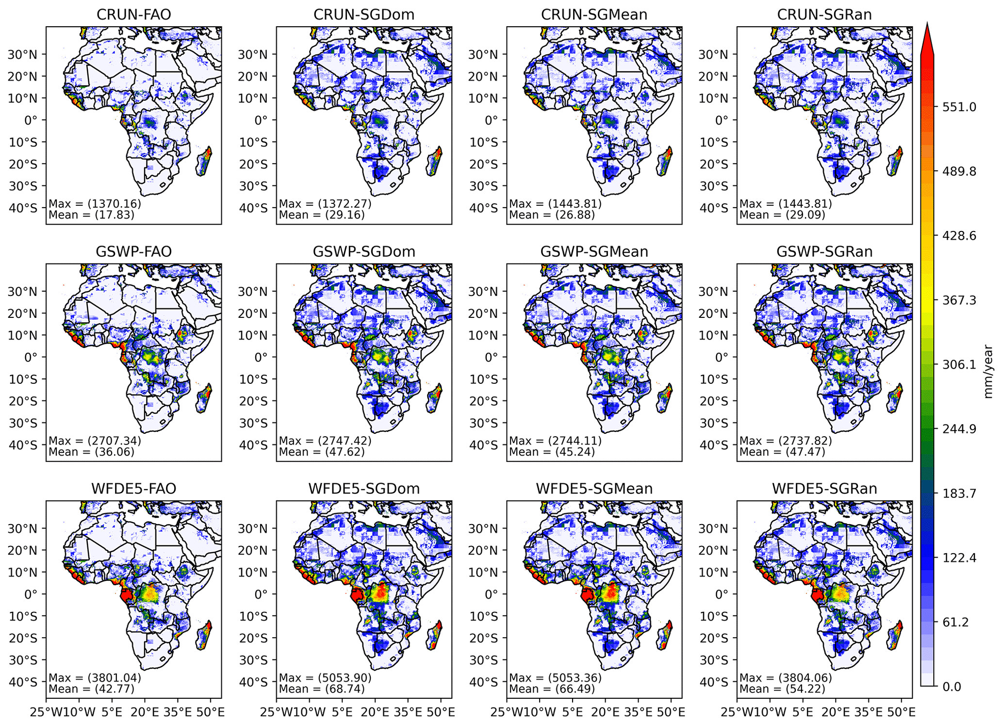
Figure 6 Spatial distribution of simulated mean annual subsurface runoff over Africa. Upper row: CRUNCEP-forced simulations with, from left to right, FAO, dominant, mean, and random upscaled soil texture map inputs. Middle row: like the upper row but for GSWP-forced simulations. Bottom row: like for the upper row but for WFDE5-forced simulations.

3.2.4 Soil moisture content

Soil moisture content estimates were obtained by calculating the weighted average of soil moisture content over the top 2 m of the soil profile in CLM5. Mean annual maxima and averages have also been analysed for each season as seasonal analysis of soil moisture content reflects seasonal changes in hydrological processes (Myeni et al., 2019) and allows a better understanding of the relationship between vegetation and water availability (Huber et al., 2011). Specifically, for the boreal summer season (JJA), the average simulated soil moisture content across the African continent varies between 0.02 cm³ cm⁻³ in the Sahara and 0.54 cm³ cm⁻³ in both Equatorial Guinea and along the coasts of Sierra Leone among the 12 simulations (Fig. 7). The upscaled soil texture maps all give very similar continental averages of soil moisture content for the summer season. The source of the soil texture maps (FAO vs. SoilGrids) resulted in some variation in the continental soil moisture content averages. A difference map showing the difference between the SGMean (SoilGrids, mean) and the three other soil texture maps (FAO and SoilGrids, dominant (SGDom) and random (SGRan)) for the same season (Fig. S2) also clearly shows that, while there is a 0.0 cm³ cm⁻³ continental mean difference among the upscaled SoilGrids maps, there is an maximum difference of 0.19 cm³ cm⁻³, a minimum difference of −0.19 cm³ cm⁻³, and a mean continental difference of 0.01 cm³ cm⁻³ between FAO and SGMean. This suggests that the source of a soil texture map could influence the soil moisture content estimates of a land surface model more than the upscaling procedure of the soil texture information. The WFDE5 atmospheric forcings are associated with more variation in simulated soil moisture content among the four soil texture maps than the other atmospheric forcings. The mean soil moisture content and the difference maps for other seasons can be found in Figs. S3–8.

Like for ET and surface runoff, varying the atmospheric forcing impacted the continental maximum of soil moisture content more than variations in soil texture input. CRUNCEP-forced simulations (6-hourly time steps) gave lower maximum soil moisture content values (0.46–0.47 cm³ cm⁻³) than GSWP-forced simulations (3-hourly time steps; 0.51–0.53 cm³ cm⁻³) and WFDE5-forced simulations (hourly time steps; 0.50–0.54 cm³ cm⁻³). This difference is likely to be attributable to lower precipitation amounts in the CRUNCEP-forced simulations combined with slightly higher ET values in comparison to simulations with the other forcings.

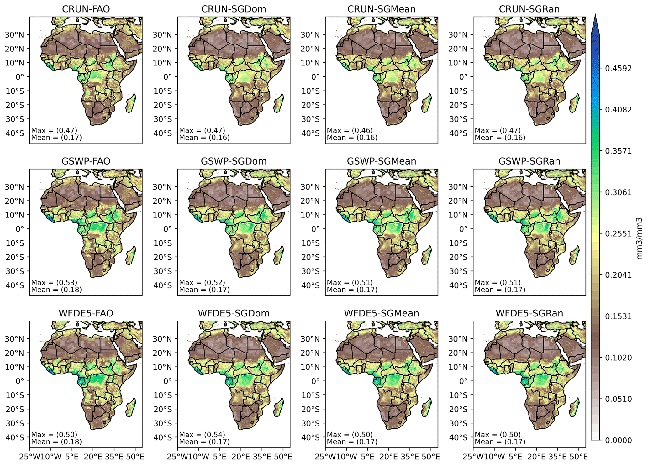
Figure 7 Spatial distribution of simulated soil moisture content in the JJA season over Africa. Top row: CRUNCEP-forced simulations with FAO and dominant, mean, and random upscaled soil texture map inputs. Middle row: like the top row but for GSWP-forced simulations. Bottom row: like the top row but for WFDE5-forced simulations.

3.3 Regional results

We present results for two regions (the Sahara and Central Africa) based on their moisture availability contrast.

3.3.1 Sahara region

The Sahara region is generally the most moisture-deficient region in Africa. Rainfall over the region was highest in August 2013 (around 30 mm per month) and was near 0 mm per month for many other months, especially in the winter season (see Fig. 8, upper row).

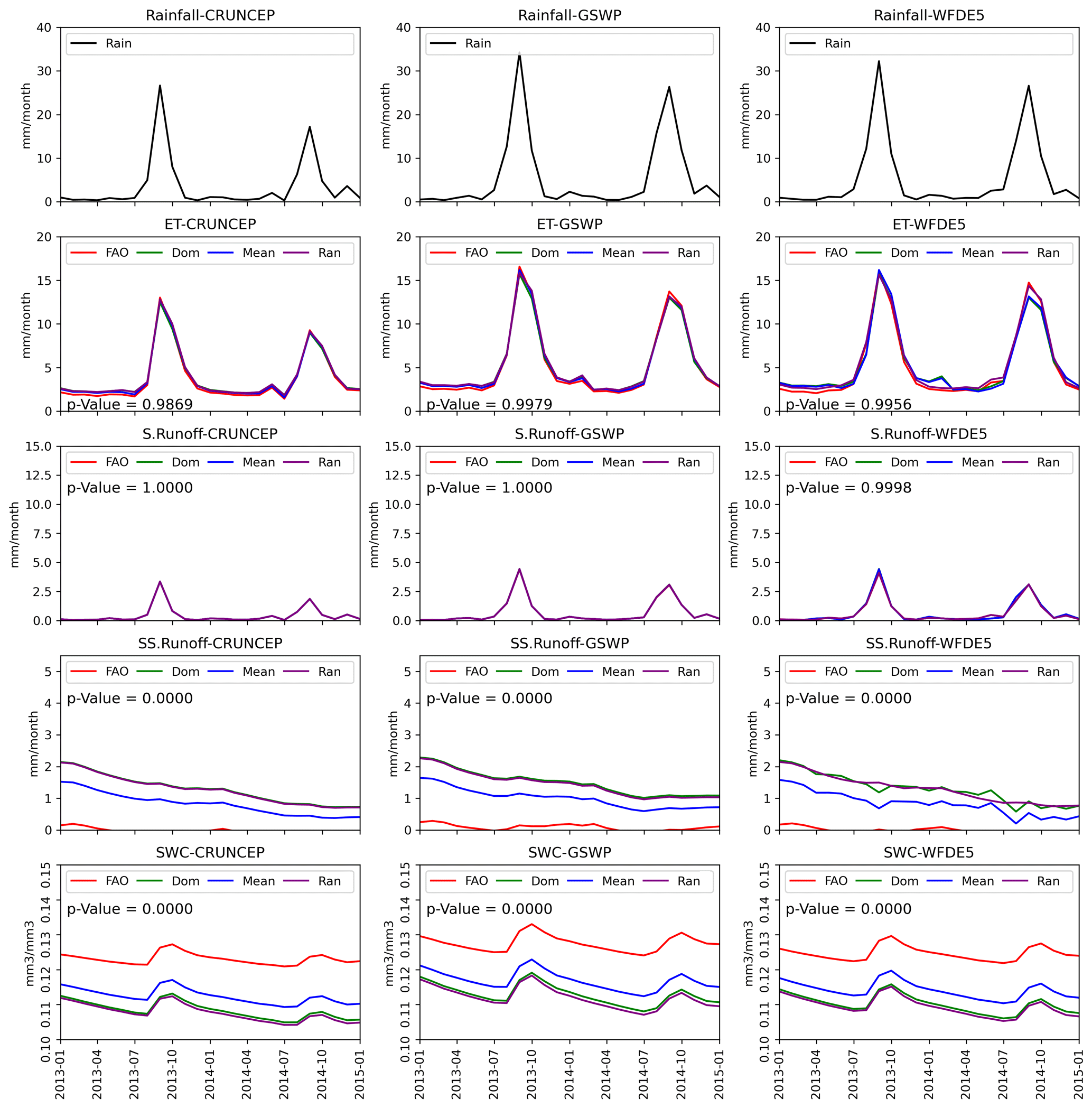
Figure 8 Monthly regional mean of water balance components over the Sahara. The p values indicate the statistical significance of the variations observed in the model outputs. The first to the fifth rows show precipitation, actual ET, surface runoff, subsurface runoff, and soil moisture content, respectively. Left, middle, and right columns show the same variables for CRUNCEP, GSWP, and WFDE5 atmospheric forcings, respectively. The lines in the figures represent results for different soil textures as input. Red line: FAO; green line: SoilGrids (dominant); blue line: SoilGrids (mean); and purple line: SoilGrids (random).

Simulated ET and surface runoff differed little among the different soil texture maps for the different atmospheric forcings. The average margin in actual ET among soil texture maps is only 0.4 mm per month for both the CRUNCEP and GSWP forcings and 0.8 mm per month for the WFDE5 forcing. ET simulated by the CLM5 model varied more as function of the atmospheric forcing and can, for a given soil texture map, vary by up to a few millimetres per month between different atmospheric forcings.

Simulated surface runoff exhibits similar patterns for all soil texture maps, with minimal surface runoff and slight increases during months with higher precipitation. The average monthly differences in surface runoff between the different soil texture maps are smaller than 0.1 mm per month. Subsurface runoff shows a decreasing trend, which is attributed to initially higher groundwater levels. While subsurface runoff is generally small in absolute terms, the different soil texture maps result in significantly varying relative amounts of subsurface runoff. Simulated average soil moisture content over the Sahara region is consistently low, with values around 0.12 cm³ cm⁻³. These significantly different values, which are not extremely low despite very limited precipitation, could be attributed to the amount of loamy soil over the region (Fig. S10), with higher residual soil moisture content than in sandy soils. Differences in simulated soil moisture content among the soil texture maps are primarily influenced by the variations in soil properties used in each map.

The different soil texture inputs into the WFDE5-forced simulations result in larger differences in simulated ET and surface runoff (though these are not significant according to ANOVA) compared to the other atmospheric forcings for regions with low soil moisture content like the Mediterranean (Fig. S12) and southwestern Africa (Fig. S16). The higher temporal resolution (1 h) of the WFDE5 atmospheric forcing leads to varying surface runoff compared to forcings with lower temporal resolutions (3 h or 6 h).

Overall, these findings over the Sahara and other low-moisture regions like the Mediterranean and southwestern Africa highlight some influence of atmospheric forcing and its temporal resolution; soil texture map variations; and their interactions in the simulation of ET, surface runoff, subsurface runoff, and soil moisture content across different regions of Africa.

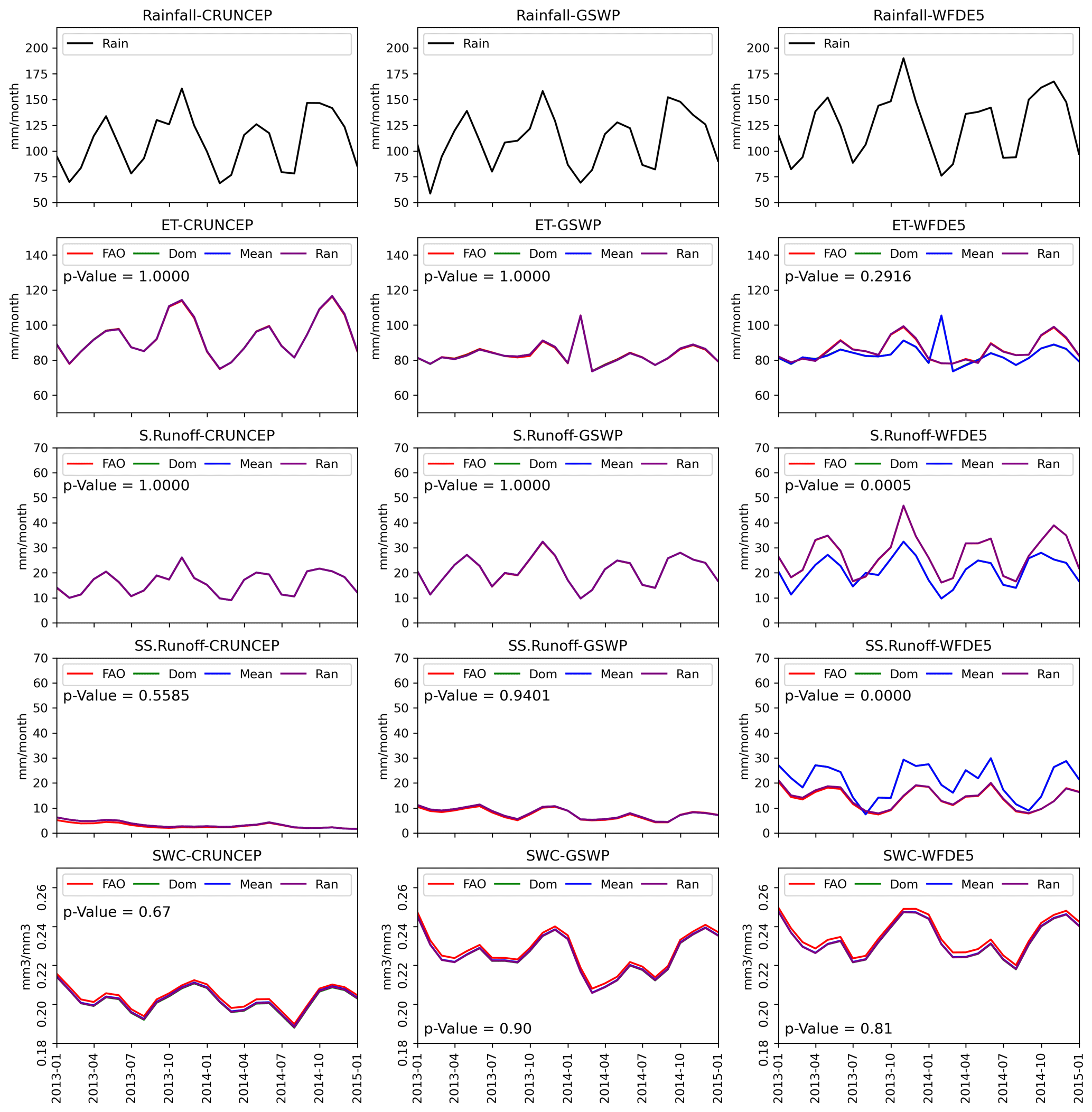
Figure 9 Monthly regional mean of water balance components over Central Africa. The p values indicate the statistical significance of the variations observed in the model outputs. Left, middle, and right columns show the same variables for CRUNCEP, GSWP, and WFDE5 atmospheric forcings, respectively. The lines in the figures represent results for different soil textures as input. Red line: FAO; green line: SoilGrids (dominant), blue line: SoilGrids (mean); and purple line: SoilGrids (random).

3.3.2 Central Africa

Central Africa encompasses the Congo rainforest, the second-largest rainforest in the world, consisting of evergreen and semi-evergreen deciduous forests (Aloysius and Saiers, 2017), and stands out as one of the most moisture-rich regions in Africa, characterized by a regional mean rainfall ranging from 50 to 200 mm per month. The proximity to the Equator results in frequent rainfall events due to recurrent convective precipitation events. The dense vegetation in Central Africa contributes to high transpiration rates, which are supported by the substantial amounts of rainfall.

Once again, we observe that only the WFDE5 atmospheric forcings exhibit a variation (not significant) in ET values across different soil texture maps, as shown in Fig. 9. On average (over the years 2013 and 2014), the soil texture maps with the highest and lowest monthly averaged ET differ by 0.5 mm per month for CRUNCEP and GSWP but by 5.8 mm per month for WFDE5. The monthly averaged surface runoff values for CRUNCEP and GSWP show little variation among different soil texture maps. However, for WFDE5, the SoilGrids map upscaled with random selection results, on average, in a significantly higher surface runoff (6.7 mm per month) than the other soil texture maps. Regarding subsurface runoff, GSWP and CRUNCEP simulations exhibit, at most, a 0.4 mm per month difference in average monthly subsurface runoff among different soil texture maps, whereas WFDE5 shows a significant difference of 7.0 mm per month. The soil moisture content maps display nearly similar average values across all atmospheric forcings and soil texture maps, with no significant differences.

Other moisture-rich regions including West Africa (Fig. S13), northeastern Africa (Fig. S14), central East Africa (Fig. S15), and southeastern Africa (Fig. S17) also show that WFDE5-forced simulations resulted in clear differences which are mostly closer to significance than GSWP and CRUNCEP in terms of simulated ET, surface runoff, and subsurface runoff for the different soil texture inputs. On the other hand, soil moisture content did not show clear significant differences for the different soil texture maps in all regions.

3.4 Local results

We now look at the results at the local scale (grid scale) to analyse further the impact of the variation in soil texture maps and atmospheric forcings on simulation outcomes. We selected one location for each of the eight climate regions: Cairo (Egypt, Mediterranean), Agadez (Niger, Sahara), Abuja (Nigeria, West Africa), Addis Ababa (Ethiopia, northeastern Africa), Salong (Democratic Republic of Congo, Central Africa), Dar es Salaam (Tanzania, central East Africa), Windhoek (Namibia, southwestern Africa), and Maseru (Lesotho, southeastern Africa). Two of the eight locations are discussed due to their contrasting moisture availability, while other locations are available in the Supplement.

3.4.1 Agadez

Agadez, situated at 16.97° N and 7.98° E, experienced its highest precipitation of 125 mm per month in August 2013 and received no rainfall during several winter months within our reference period. The grid cell in focus is also dominated by sandy and loamy soils according to all four soil texture maps. The results for Agadez indicate a close association between ET peaks and precipitation peaks as ET in this region, the Sahara, is limited by water availability. Despite a 5-month period without rainfall from September 2013 to January 2014, ET values in Agadez remained at nonzero (1.5 mm per month) between January 2014 and April 2014. This can be attributed to irrigation practices automatically applied to sustain irrigated crops when the soil moisture content falls below a critical threshold within CLM5.

The WFDE5-forced simulations for Agadez (Fig. 10) show that different (upscaled) soil texture maps yield varying monthly ET, surface runoff, and subsurface runoff values. On average (over the years 2013 and 2014), the soil texture maps with the highest and lowest monthly averaged ET differ by 0.7 mm per month for CRUNCEP, 0.9 mm per month for GSWP, and 1.8 mm per month for WFDE5 (though this is not significant according to ANOVA). This can be attributed to low rainfall. Model simulations driven by CRUNCEP or GSWP show no variation in surface runoff as function of the soil texture map, while slight but insignificant variations in surface runoff are found for WFDE5. A similar pattern is observed for subsurface runoff. Although the texture class for the dominant and mean SoilGrids is loamy sand (LS) and that for FAO and the random SoilGrids is sandy loam (SL) for the grid cell in question (Table S17), statistically significant differences in soil water content are observed among the four soil texture maps. These differences arise because, although the soil texture classes are similar, the proportions of clay, sand, and silt vary among the four maps, resulting in different hydraulic conductivities.

Overall, the results for Agadez demonstrate the influence of soil texture map variation on ET, surface runoff, and subsurface runoff, with WFDE5 simulations exhibiting more pronounced variations compared to CRUNCEP and GSWP forcings. These findings underscore the importance of soil texture representation and the temporal resolution of the atmospheric forcing in capturing the hydrological processes in Agadez and similar locations.

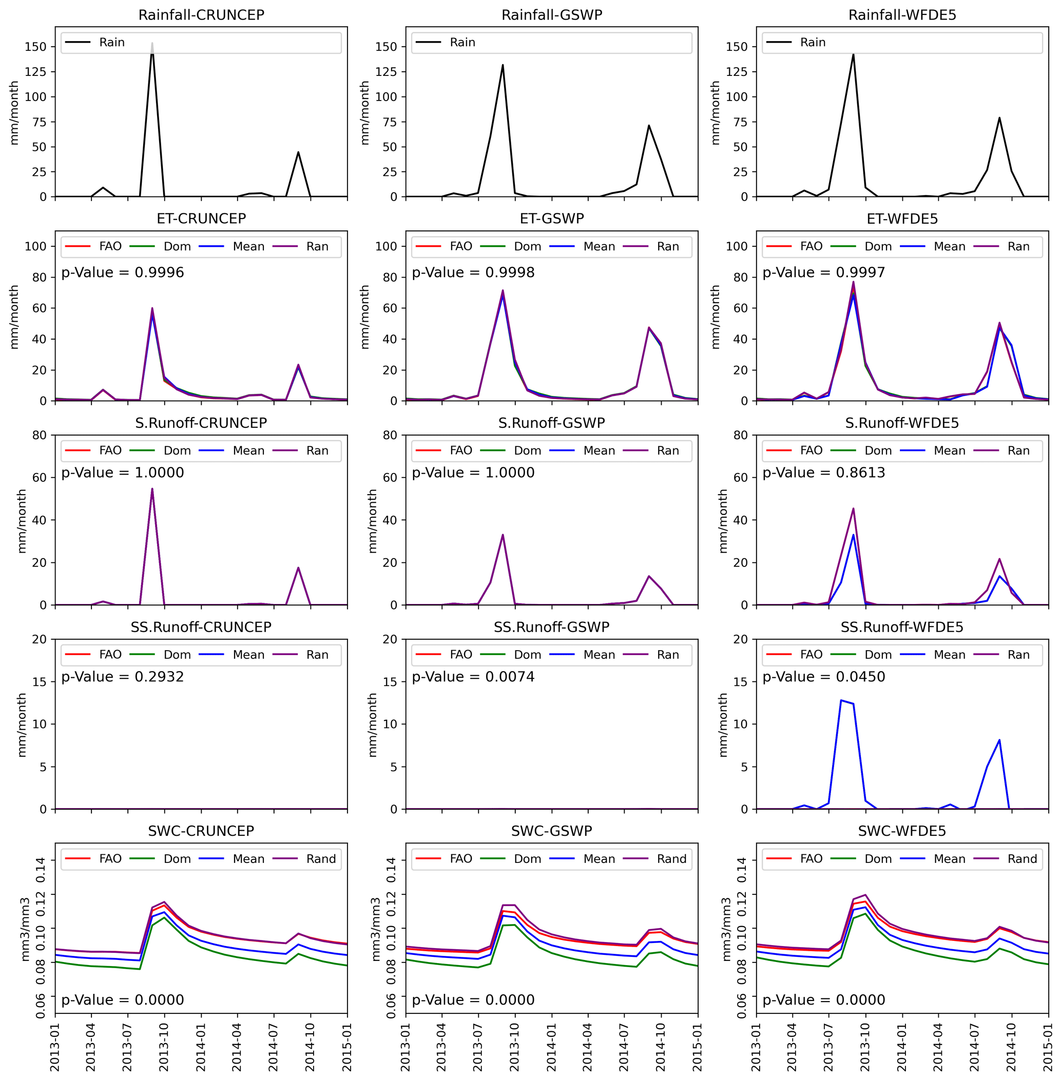
Figure 10 Monthly local estimates of water balance components over Agadez. The p values indicate the statistical significance of the variations observed in the model outputs. Left, middle, and right columns show the same variables for CRUNCEP, GSWP, and WFDE5 atmospheric forcings, respectively. The lines in the figures represent results for different soil textures as input. Red line: FAO; green line: SoilGrids (dominant); blue line: SoilGrids (mean); and purple line: SoilGrids (random).

3.4.2 Abuja

Abuja, situated in Nigeria at coordinates of 9.07° N, 7.30° E, exhibits a distinct yearly precipitation cycle characterized by high rainfall during the summer months, with precipitation exceeding 200 mm per month. Conversely, the winter season is dry, with months devoid of any rainfall (Fig. 11). ET peaks in Abuja typically occur approximately 1 month or more after the peak of rainfall, as observed in 2014.

Simulated ET, surface runoff, and subsurface runoff in Abuja demonstrate variations across different soil texture maps, although these are not statistically significant; these are particularly noticeable with the high-temporal-resolution atmospheric forcings provided by WFDE5. In terms of ET, WFDE5 displays the highest mean margin differences among soil texture maps (10.4 mm per month), followed by GSWP (1.4 mm per month) and CRUNCEP (1.0 mm per month). Regarding surface runoff, WFDE5 also yields the highest mean margin (7.5 mm per month), while CRUNCEP and GSWP exhibit negligible differences (< 0.2 mm per month). Similarly, the ranking of differences in subsurface runoff follows the same pattern, with WFDE5 showing the largest disparities (7.7 mm per month), followed by GSWP (0.4 mm per month) and, finally, CRUNCEP (0.0 mm per month). Notably, the FAO soil texture map consistently results in slightly higher soil moisture content (SWC) compared to the SoilGrids soil texture maps for all atmospheric forcings (as depicted in the lower row of Fig. 8). However, these differences in SWC do not exceed 0.01 cm³ cm⁻³ across all atmospheric forcings and are valued as insignificant according to ANOVA.

Similar patterns are observed for other locations, including Cairo (Fig. S18), Addis Ababa (Fig. S19), Salong (Fig. S20), Dar es Salaam (Fig. S21), Windhoek (Fig. S22), and Maseru (Fig. S23). WFDE5-forced simulations exhibit larger variations in simulated ET, surface runoff, and subsurface runoff among different soil texture maps compared to the other atmospheric forcings. Simulated soil moisture content shows minimal variations among the different soil texture maps for a given atmospheric forcing.

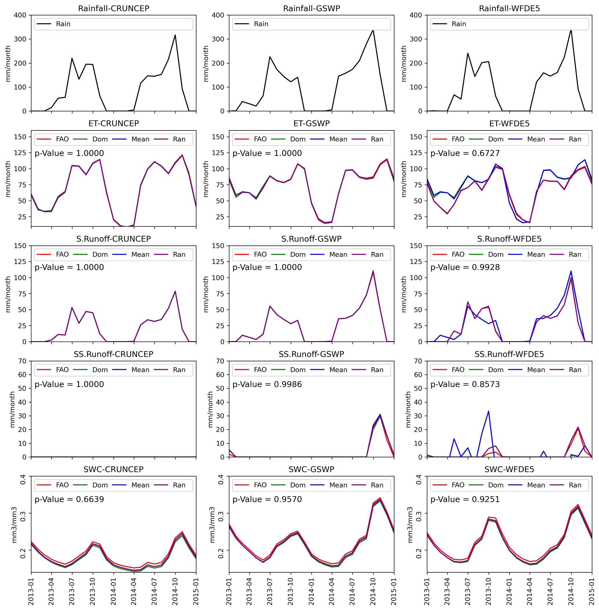
Figure 11 Monthly local estimates of water balance components over Abuja. The p values indicate the statistical significance of the variations observed in the model outputs. Left, middle, and right columns show the same variables for CRUNCEP, GSWP, and WFDE5 atmospheric forcings, respectively. The lines in the figures represent results for different soil textures as input. Red line: FAO; green line: SoilGrids (dominant); blue line: SoilGrids (mean); and purple line: SoilGrids (random).

3.4.3 Aggregation of WFDE5 to 3-hourly and 6-hourly resolutions

To further validate the role of the temporal resolution of atmospheric forcings, WFDE5 forcing was aggregated (from hourly data) to 3-hourly and 6-hourly resolutions so that it varied temporally only on a 3-hourly and 6-hourly basis, like GSWP and CRUNCEP. Simulations were performed to examine the impact of the new temporal resolution on ET, surface runoff, subsurface runoff, and soil moisture content both regionally and locally. We compare CRUNCEP (6-hourly), 6H-WFDE5 (6-hourly), 3H-WFDE5 (3-hourly), GSWP (3-hourly), and WFDE5 (1-hourly).

Table 3 Mean margin of simulated variables among soil texture maps for CRUNCEP (6-hourly), GSWP (3-hourly), 6H-WFDE5 (6-hourly), 3H-WFDE5 (3-hourly), and WFDE5 (1-hourly).

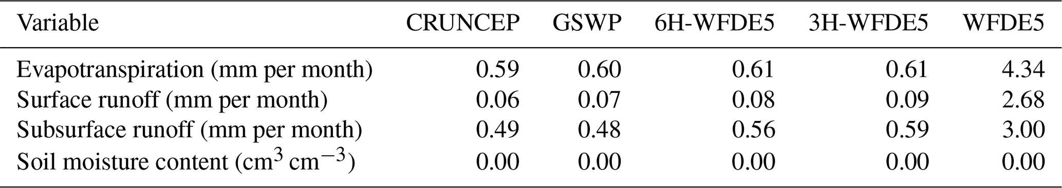
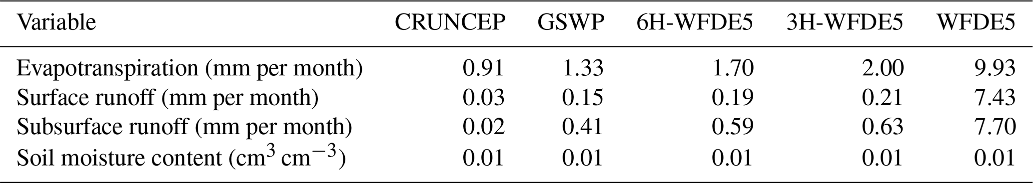
Table 3 shows the impact of varying soil texture map inputs on different water balance component for West Africa. Simulated variables show much less variation as a function of soil texture map input for CRUNCEP, GSWP, 6-hourly aggregated WFDE5 forcings, and 3-hourly aggregated WFDE5 forcings compared to 1-hourly WFDE5 forcings. Similar results are found for Abuja (Table 4), where CRUNCEP, GSWP, 6H-WFDE5, and 3H-WFDE5 forcings produce variations between 0.02 and 2.0 mm per month in ET, surface runoff, and subsurface runoff as a function of the soil texture map, while WFDE5 produces variations between 7.43 and 9.93 mm per month among soil texture maps. A similar observation was also made for other regions (Tables S1, S2, S4, S5, S6, S7, and S8) and locations (grid cells) (Tables S9, S10, S11, S12, S13, S14, S15, and S16).

Table 4 Mean margin of simulated variables among soil texture maps for CRUNCEP (6-hourly), GSWP (3-hourly), 6H-WFDE5 (6-hourly), 3H-WFDE5 (3-hourly), and WFDE5 (1-hourly).

3.5 Discussion

The simulation results over Africa suggest that the atmospheric forcings exert an important control on the ET estimates, while soil texture is important for simulating surface and subsurface runoff. The simulation results also suggest that the temporal resolution of atmospheric forcings influences the simulation outcomes, especially surface and subsurface runoff, and the interaction with soil texture seems to play a role here. These findings agree with the work of Zhang et al. (2023) on the role of soil texture and the work of Beusekom et al. (2022) on the impact of temporal forcing aggregation on land surface model outputs.

The analysis of water budget components shows differences in simulated ET, surface runoff, and subsurface runoff for the different upscaled soil texture maps in combination with WFDE5-forced simulations but not in combination with other atmospheric forcings with more coarse temporal resolutions. We observed for ET and surface runoff across all regions that a higher temporal resolution led to higher differences in ET and surface runoff between soil texture map outcomes, with the largest differences for WFDE5 (hourly resolution), followed by GSWP (3-hourly resolution) and CRUNCEP (6-hourly resolution). For subsurface runoff, a higher temporal resolution did not result in such a systematic pattern in moisture-rich regions with rainfall above 200 mm per month. However, in moisture-deficient regions, a higher temporal resolution of the atmospheric forcing is associated with more variation in subsurface runoff for different soil texture maps. The temporal resolution of the atmospheric forcings did not result in different soil moisture content results for each soil texture map, but in all regions, it was observed that the FAO soil texture map resulted in different soil moisture content than the SoilGrids250m soil texture maps, partially confirming the findings of Tafasca et al. (2020), which showed that soil mapping had a stronger influence on soil moisture content compared to fluxes.

3.5.1 The role of temporal resolution in rainfall intensity representation

We investigated whether the higher temporal resolution of simulations influenced the rainfall partitioning into surface runoff and infiltration. The absolute monthly (Figs. S26 and S27) and annual (Fig. S9) precipitation amounts over the continent vary only slightly among CRUNCEP, GSWP, and WFDE5. The spatial averages for annual precipitation are 608, 638, and 666 mm yr⁻¹ for CRUNCEP, GSWP, and WFDE5 respectively. These differences in rainfall amount do not explain why only WFDE5 soil texture variations result in larger runoff and evapotranspiration variations. We also analysed the number of precipitation events with a rainfall intensity above 3 mm h⁻¹ for each of the three atmospheric forcings and eight selected locations. We found that WFDE5 had a much higher number of precipitation events with rainfall intensity greater than 3 mm h⁻¹ than both CRUNCEP and GSWP at all eight locations (see Table S17), indicating a better representation of rainfall intensity. GSWP and CRUNCEP had more rainfall events with much lower intensities. This indicates that rainfall intensity representation and its impact on the partitioning between infiltration and surface runoff in the land surface model is a likely reason for the higher sensitivity of model outcomes to soil texture input in WFDE5-forced simulations than in GSWP- and CRUNCEP-forced simulations.

3.5.2 The role of soil texture in water balance components

Rainfall intensity has a stronger influence on surface runoff generation than rainfall amount (e.g. Jungerius and ten Harkel, 1994; Yao et al., 2021), and surface runoff is, on the other hand, also strongly influenced by the hydraulic conductivity, with lower conductivity supporting higher surface runoff (Suryatmojo and Kosugi, 2021; Ow and Chow, 2021; Chandler et al., 2018). Therefore, for WFDE5 forcings, there are potentially more situations with surface runoff, such that the role of different soil properties can come into play. We analysed this for all eight locations (Fig. S53) by calculating the standard deviation of the fraction of precipitation turned into surface runoff among the four soil texture maps for each atmospheric forcing. For the WFDE5 atmospheric forcings, this standard deviation varies between 1.2 % of rainfall for Dar es Salaam and 10.1 % of rainfall in Addis Ababa, while the standard deviations are less than 0.4 % for both CRUNCEP (6-hourly) and GSWP (3-hourly) atmospheric forcings for all locations. This identified impact of surface runoff agrees with Mizuochi et al. (2021) for the ORCHIDEE model and with Fersch et al. (2020) for the WRF-Hydro model. This shows that the soil texture information has a control over the partitioning of fluxes for higher-temporal-resolution atmospheric forcings (Shuai et al., 2022). Since surface runoff and infiltration are sensitive to rainfall intensity (Mertens et al., 2002) and since soil texture determines saturated hydraulic conductivity, the timings of runoff (Hammond et al., 2019), surface runoff, and subsurface runoff vary as a function of soil texture inputs into the WFDE5 simulations (mainly at the local and regional scales).

3.5.3 Implications for land surface modelling and community impact

This work demonstrates the critical role that high-resolution soil texture information and higher-temporal-resolution forcing datasets play in simulating water balance components. It highlights the need to use higher-resolution soil texture information in land surface model simulations to improve the capturing of grid- and sub-grid-scale land surface heterogeneity. It is also necessary to provide better pedotransfer functions which link soil texture and soil hydraulic parameters which ultimately control infiltration. The higher temporal resolution of atmospheric forcing (hourly) in this work has also captured water balance dynamics differently compared to coarse-temporal-resolution atmospheric forcing, which indicates a need for the community to further strengthen research to improve the temporal resolution of atmospheric forcings, especially over Africa. There have been advances in improving the spatial resolution of atmospheric forcings (e.g. Funk et al., 2015), but this work serves as an indicator that higher-temporal-resolution atmospheric forcings are also needed. The works of Hersbach et al. (2020) and Cucchi et al. (2020) must be complemented in producing a higher temporal resolution of atmospheric forcings. This advancement can eliminate the need for temporal disaggregation of precipitation, as done in this work. This work showed that soil texture information is important in combination with a high temporal resolution of atmospheric forcings as it impacts the division of rainfall into surface runoff and infiltration. Ultimately, land surface models also need to be better tuned to correctly reproduce this division in the context of the higher temporal resolution of atmospheric input data and the higher spatial resolution of information on soil hydraulic properties.

4 Conclusions

Community Land Model version 5 (CLM5) model runs over the African continent were performed at a high spatial resolution of approximately 3 km, with four different soil texture maps and three different atmospheric forcings. The four different soil texture inputs included the FAO soil map and three differently upscaled SoilGrids250 maps. The three different atmospheric forcings were CRUNCEPv7, GSWP3, and WFDE5. The most important findings were as follows: average evapotranspiration and surface runoff simulated by CLM5 over the African continent show a limited sensitivity to variations in the soil texture input. The source of soil texture information (FAO versus SoilGrids) results only in minor variations in the continental average ET or surface runoff (0.3 % variations around mean), and the impact of different upscaling approaches of soil texture information is even smaller. This sensitivity to soil texture input is much smaller than the sensitivity to the different atmospheric forcings (3 % variation for mean ET and 26 % variation for surface runoff). Average subsurface runoff and average soil moisture at the continental scale are both as sensitive to variations in atmospheric forcings as they are to variations in soil texture information.

Although average surface runoff at the continental scale shows a limited sensitivity to soil texture input, at the regional and, especially, the local scale, this sensitivity is much higher, but this is mainly so in combination with the higher temporal resolution of WFDE5 forcings (hourly). The higher temporal resolution of WFDE5 forcings (hourly) compared to the other atmospheric forcings resulted in larger variations not only in simulated surface runoff but also in ET and subsurface runoff for the different soil texture maps. This points to the fact that the impact of soil texture becomes more important in combination with the higher temporal resolution of atmospheric forcings. We explain this with the impact of the temporal resolution of atmospheric forcings on the rainfall intensity and the partitioning of rainfall into surface runoff, which is also determined by the hydraulic conductivity of the soil. This, in turn, also affects the amount of water available for evapotranspiration and drainage.

This study therefore recommends further advances in the provision of both higher-temporal-resolution climate datasets and higher-spatial-resolution soil information over Africa. With higher-spatial-resolution soil information, sub-grid-scale land surface heterogeneity will be handled with more accuracy. Also, higher-temporal-resolution climate datasets at less than 1 h time steps will not only eliminate the need for temporal disaggregation in land surface model applications but will also ensure that more accurate atmospheric variables are supplied to the land surface model at each time step.

This study also highlights specific implications for the simulation of surface runoff by land surface models. A higher spatial resolution of soil texture data or of soil hydraulic properties at finer spatial scales will potentially allow for a better modelling of surface runoff and, subsequently, of other water balance components in each grid cell. In addition, higher-temporal-resolution atmospheric forcing captures high-intensity rainfall events that can produce more surface runoff in a short period of time, especially on soils with low hydraulic conductivity, leading to a more accurate estimate of surface runoff in each affected grid cell.

It is assumed in this work that model shortcomings (for example, those related to the representation of yearly vegetation cycles and the representation of different crop types) do not substantially affect the differences in the simulation results. Furthermore, the release of CLM5 as used in this work assumes 16 plant functional types for the African continent by default, which does not represent all vegetation types. Also, irrigation is hard-coded into the surface datasets. Future work should reduce these limitations.