CH-RUN: a deep-learning-based spatially contiguous runoff reconstruction for Switzerland

This study presents a data-driven reconstruction of daily runoff that covers the entirety of Switzerland over an extensive period from 1962 to 2023. To this end, we harness the capabilities of deep-learning-based models to learn complex runoff-generating processes directly from observations, thereby facilitating efficient large-scale simulation of runoff rates at ungauged locations. We test two sequential deep-learning architectures: a long short-term memory (LSTM) model, which is a recurrent neural network able to learn complex temporal features from sequences, and a convolution-based model, which learns temporal dependencies via 1D convolutions in the time domain. The models receive temperature, precipitation, and static catchment properties as input. By driving the resulting model with gridded temperature and precipitation data available since the 1960s, we provide a spatiotemporally continuous reconstruction of runoff. The efficacy of the developed model is thoroughly assessed through spatiotemporal cross-validation and compared against a distributed hydrological model used operationally in Switzerland.

The developed data-driven model demonstrates not only competitive performance, but also notable improvements over traditional hydrological modeling in replicating daily runoff patterns, capturing interannual variability, and discerning long-term trends. The resulting long-term reconstruction of runoff is subsequently used to delineate substantial shifts in Swiss water resources throughout the past decades. These are characterized by an increased occurrence of dry years, contributing to a negative decadal trend in runoff, particularly during the summer months. These insights are pivotal for the understanding and management of water resources, particularly in the context of climate change and environmental conservation. The reconstruction product is made available online.

Furthermore, the low data requirements and computational efficiency of our model pave the way for simulating diverse scenarios and conducting comprehensive climate attribution studies. This represents a substantial progression in the field, allowing for the analysis of thousands of scenarios in a time frame significantly shorter than those of traditional methods.

1 Introduction

Hydrological modeling and runoff prediction are critical for understanding and managing water resources, particularly in the face of climate change and increasing human impacts on the environment (Seneviratne et al., 2021; Arias et al., 2023). In Switzerland, a country characterized by diverse topography and climatic conditions, understanding and predicting runoff patterns is essential for effective water management, flood control, and environmental conservation (Brunner et al., 2019a).

Traditional hydrological models offer pivotal insights into land surface processes. For Switzerland, a diverse array of hydrological models has been employed (Horton et al., 2022), ranging from complex ones, which are heavily founded on physical principles, to lightweight ones using conceptual process representations with calibrated parameters. While the former offer detailed insights and control, they rely on a large number of inputs and are computationally expensive. The latter, in contrast, can be parsimonious in terms of data and computational resources, yet they need to be calibrated per catchment, which limits their applicability to prediction in ungauged catchments. Generalization to ungauged catchments via regionalization is possible but introduces another layer of complexity (Beck et al., 2016). As a complementary approach, deep learning holds potential as a tool for hydrological modeling in terms of both performance and efficiency (Nearing et al., 2021), and it comes with built-in regionalization when trained jointly on multiple catchments (Kratzert et al., 2024).

The potential of machine learning to represent land surface processes, including runoff, has been widely demonstrated and discussed (Camps-Valls et al., 2021; Reichstein et al., 2018; Kraft et al., 2019; Gudmundsson and Seneviratne, 2015; Ghiggi et al., 2021). Deep learning, in particular, has shown promise for nowcasting and forecasting runoff in gauged catchments, aiding in warning systems for extreme flow events (Kratzert et al., 2018; Gauch et al., 2021a). It is, however, less common to employ data-driven models for large-scale reconstruction and monitoring (Nasreen et al., 2022). Reconstruction products are widely used for process understanding, investigation of long-term trends, and study of extreme events within a wider spatiotemporal context (Gudmundsson and Seneviratne, 2015; Ghiggi et al., 2019, 2021; Muelchi et al., 2022). In addition, machine-learning-based models enable simulation of scenarios and real-time monitoring with significant speedup (Reichstein et al., 2019; Kraft et al., 2021).

This study introduces a data-driven approach to reconstructing daily runoff in Switzerland with contiguous spatial coverage, spanning an extensive period from 1962 to 2023 with the potential for continuous updates. We optimize a range of neural-network-based models in different setups and evaluate their performance at the catchment level in a comprehensive spatiotemporal cross-validation scheme. The results are benchmarked against simulations from the PREVAH (PREecipitation-Runoff-EVApotranspiration Hydrological) model, which is used operationally in Switzerland. The extended coverage compared to PREVAH is enabled by reduced data requirements by only using temperature and precipitation as meteorological drivers. In the Swiss context, these variables cover the period from the 1960s onward as regular grids, while additional variables, such as relative humidity and wind speed, are available from the 1980s. The best-performing model has subsequently been used to reconstruct daily runoff rates with complete spatiotemporal coverage since the 1960s. The paper closes with a discussion of the strengths and limitations of the approach and the first insights from the extended reconstruction.

2 Data

2.1 Runoff observations

The observed discharges were taken from the CAMELS-CH dataset (Höge et al., 2023), which was updated with current data from the Swiss Federal Office for the Environment (FOEN, 2024) and supplemented by stations operated by the cantons Aargau, Baselland, Bern, St. Gallen, and Zurich. In total, 267 stations were available. A subset of 98 catchments was selected to minimize the anthropogenic impact (Fig. 1); i.e., no hydropower plant or reservoir was located upstream of the gauging station. This selection was based on the attributes of the CAMELS-CH dataset and insights from a previous study (Brunner et al., 2019c).

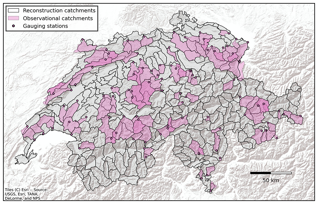
Figure 1 From sparse observations with low anthropogenic impact on contiguous spatial coverage, the 98 observational catchments highlighted in magenta were selected to be only marginally affected by anthropogenic factors and served as a basis for training and evaluating the data-driven models. These catchments are of similar sizes to the target catchments for reconstruction (grey).

2.2 Meteorological drivers

We considered daily precipitation and air temperature to be meteorological drivers from interpolated observational data with a spatial resolution of 1 km, i.e., the daily gridded datasets RhiresD (Schwarb, 2000; MeteoSwiss, 2021a) and TabsD (Frei, 2014; MeteoSwiss, 2021b). Gridded daily temperature and precipitation were spatially averaged for all the considered catchments.

2.3 Catchment properties

For the across-catchment modeling of runoff, a set of static catchment properties was considered. These variables can improve generalization to catchments not seen during training. The static variables used are identical to those needed to force the spatially distributed PREVAH model (see the next section) and include elevation, aspect, land use, soil depth, soil water holding capacity, hydraulic conductivity, and two further indices describing soil and hydraulic properties. These gridded variables were aggregated to appropriate catchment values depending on the level of measurement, e.g., a circular mean for aspect or a distribution of classes within each catchment for land use. As compared to previous applications of PREVAH (Viviroli et al., 2009b; Speich et al., 2015), the sources of the data providing the static properties have been updated and include the following:

• the swissALTI3D digital elevation model (swisstopo, 2018; Weidmann et al., 2018);

• the new habitat map of Switzerland (Price et al., 2023), aggregated to match the land use classes integrated into PREVAH;

• the SoilGrids products (Hengl et al., 2017; Poggio et al., 2021), enriched with high-resolution data for Swiss forests (Baltensweiler et al., 2022) and merged and used to estimate soil properties; and

• the recent information on the extent of glaciers in Switzerland (Linsbauer et al., 2021).

2.4 PREVAH runoff simulations as a benchmark

The modeling of Swiss catchments has a long history in hydrology research (Horton et al., 2022; Addor and Melsen, 2019). Among a set of 21 models compared, Horton et al. (2022) found the PREVAH model (Viviroli et al., 2009b) to be the most commonly used one, with applications going from the plot-scale process evaluation (Zappa and Gurtz, 2003) to the operational implementation for drought anticipation (Bogner et al., 2022) and to the Switzerland-wide assessment of climate impacts on hydrology (Brunner et al., 2019a). Furthermore, a PREVAH-based baseline is included in the Swiss version of the CAMELS (Höge et al., 2023) dataset (catchment attributes and meteorology for large-sample studies) as introduced by Addor et al. (2017).

For this study, we created a benchmark runoff simulation for the selected catchments on the basis of PREVAH. The simulations cover the period from 1981 until the end of 2022. The procedure adopted to obtain the PREVAH benchmark closely follows the methodologies presented in previous studies (Speich et al., 2015; Brunner et al., 2019c; Höge et al., 2023). The gridded version of PREVAH (Viviroli et al., 2009b; Speich et al., 2015) has been applied at 500 m resolution. The time series of the investigated catchments were then obtained by spatially averaging daily gridded values. For further details on the setup and application of PREVAH, we refer the reader to the references provided above. For the present study it is nevertheless important to know that the gridded simulations at 500 m×500 m resolution have not been specifically recalibrated for the catchments investigated. Instead, the spatially explicit version of PREVAH accesses a previously calibrated set of model parameters covering Switzerland that have been estimated using a regionalization approach (Viviroli et al., 2009c, a; Köplin et al., 2010). We also note that runoff rates from PREVAH are to be considered the natural response of the grids within the catchments investigated, without any considerations of water diversions for hydropower, flood damping by (regulated) lakes, or any kind of water use (Brunner et al., 2019d).

3 Methods

3.1 Neural network architectures

We used two classes of temporal neural network models for runoff modeling, i.e., the long short-term memory (LSTM; Hochreiter and Schmidhuber, 1997) model and the temporal convolutional network (TCN; Bai et al., 2018). While the LSTM model maintains an internal state that is updated dynamically, the TCN is based on a sparse and efficient 1D convolution in the time domain. The latter is parallelizable in time and therefore computationally more efficient. We employ three approaches, described hereafter, to fuse the dynamic meteorological variables x_t,c at time t and catchment c with the static variables s_c, independent of the temporal model used. The selection of the best fusion approach was part of the hyperparameter tuning (Sect. 3.3) and was performed independently of the model setup described in Sect. 3.5. Note that the following description of the model architectures is simplified and that the actual setup uses vectorized and efficient computation.

3.1.1 Pre-fusion with encoding

In the first approach, which we called pre-fusion with encoding, ${\mathit{x}}_{t,c}\in {\mathbb{R}}^M$ (a vector of M meteorological features) and s_c∈ℝ^S (a vector of S static features) are, as part of the model training, encoded into ${\mathit{e}}_{t,c}\in {\mathbb{R}}^D$, i.e., into a vector of length D (the model dimensionality). The encoding is done using the stacked feed-forward neural network layers $f_{{\text{NN}}_{\mathrm{1}}}$ and $f_{{\text{NN}}_{\mathrm{2}}}$, respectively. The two encodings are combined by element-wise addition; i.e., static encoding is added to each meteorological encoding equally, as shown in Eq. (1). The resulting combined encoding e_t,c is then fed into one or more temporal layers f_TNN (Eq. 2), yielding the temporal encoding ${\mathit{h}}_{t,c}\in {\mathbb{R}}^D$, which is then decoded into a single value $q_{t,c}^{*}\in \mathbb{R}$ (Eq. 3) by another stack of feed-forward neural networks $f_{{\text{NN}}_{\mathrm{3}}}$.

$$\begin{array}{}\text{(1)}& {\displaystyle }\text{Feature encode}{\mathit{e}}_{t,c}& {\displaystyle }=f_{{\text{NN}}_{\mathrm{1}}}\left({\mathit{x}}_{t,c}\right)+f_{{\text{NN}}_{\mathrm{2}}}\left({\mathit{s}}_c\right)\text{(2)}& {\displaystyle }\text{Temporal encode}{\mathit{h}}_{t,c}& {\displaystyle }=f_{\text{TNN}}({\mathit{e}}_{t,c},{\mathit{e}}_{t-\mathrm{1},c},\mathrm{\dots },{\mathit{e}}_{t-k,c})\text{(3)}& {\displaystyle }\text{Output decode}{q}_{t,c}^{*}& {\displaystyle }=f_{{\text{NN}}_{\mathrm{3}}}\left({\mathit{h}}_{t,c}\right)\text{(4)}& {\displaystyle }\text{Output transform}{q}_{t,c}& {\displaystyle }=\log (\mathrm{1}+\exp (q_{t,c}^{*}\left)\right)\end{array}$$

While the LSTM model uses all the input time steps, the TCN uses the limited-context k, depending on its hyperparameters. The decoded output is then transformed into the positive domain, $q_{t,c}\in {\mathbb{R}}_{+}$, using the softplus activation, as shown in Eq. (4). This output mapping is consistent across the fusion methods.

In this fusion approach, the potentially complex interactions of the dynamic and static input variables are injected prior to the temporal layer, presumably offloading some nontemporal interaction complexity from it. Note that the selection of model characteristics, such as the number of hidden nodes and layers, was based on hyperparameter tuning (see the next section).

3.1.2 Pre-fusion with repetition

In the second approach, pre-fusion with repetition, the static vector s_c is simply repeated in time and concatenated to the temporal input x_t,c (Eq. 5). This combined encoding, based on a feed-forward neural network $f_{{\text{NN}}_{\mathrm{4}}}$, is then fed into the temporal module (Eq. 6) and mapped to the output with another neural network $f_{{\text{NN}}_{\mathrm{5}}}$ as previously described and as shown in Eqs. (7) and (8). This approach is conceptually similar to pre-fusion with encoding, but it leaves the learning of the nonlinear interactions within the static inputs to the temporal layer.

$$\begin{array}{}\text{(5)}& {\displaystyle }\text{Feature encode}{\mathit{e}}_{t,c}& {\displaystyle }=f_{{\text{NN}}_{\mathrm{4}}}\left(\right[{\mathit{x}}_{t,c},{\mathit{s}}_c\left]\right)\text{(6)}& {\displaystyle }\text{Temporal encode}{\mathit{h}}_{t,c}& {\displaystyle }=f_{\text{TNN}}({\mathit{e}}_{t,c},{\mathit{e}}_{t-\mathrm{1},c},\mathrm{\dots },{\mathit{e}}_{t-k,c})\text{(7)}& {\displaystyle }\text{Output decode}{q}_{t,c}^{*}& {\displaystyle }=f_{{\text{NN}}_{\mathrm{5}}}\left({\mathit{h}}_{t,c}\right)\text{(8)}& {\displaystyle }\text{Output transform}{q}_{t,c}& {\displaystyle }=\log (\mathrm{1}+\exp (q_{t,c}^{*}\left)\right)\end{array}$$

3.1.3 Post-fusion with repetition

Post-fusion with repetition, finally, first encodes the meteorological input x_t,c (Eq. 9) with a feed-forward neural network $f_{{\text{NN}}_{\mathrm{6}}}$ and then runs the encoding through the temporal module (Eq. 10). It then decodes the combined temporal encoding and static inputs s_c via repetition in time (Eq. 11) by $f_{{\text{NN}}_{\mathrm{7}}}$, followed by mapping to the positive domain (Eq. 12). In this approach, the dynamics learned by the temporal layers cannot be modulated by the static variables.

$$\begin{array}{}\text{(9)}& {\displaystyle }\text{Feature encode}{\mathit{e}}_{t,c}& {\displaystyle }=f_{{\text{NN}}_{\mathrm{6}}}\left({\mathit{x}}_{t,c}\right)\text{(10)}& {\displaystyle }\text{Temporal encode}{\mathit{h}}_{t,c}& {\displaystyle }=f_{\text{TNN}}({\mathit{e}}_{t,c},{\mathit{e}}_{t-\mathrm{1},c},\mathrm{\dots },{\mathit{e}}_{t-k,c})\text{(11)}& {\displaystyle }\text{Output decode}{q}_{t,c}^{*}& {\displaystyle }=f_{{\text{NN}}_{\mathrm{7}}}\left(\right[{\mathit{h}}_{t,c},{\mathit{s}}_c\left]\right)\text{(12)}& {\displaystyle }\text{Output transform}{q}_{t,c}& {\displaystyle }=\log (\mathrm{1}+\exp (q_{t,c}^{*}\left)\right)\end{array}$$

3.2 Model training and hyperparameter tuning

3.2.1 Data transformation

We transformed both the dynamic and static input features using Z transformation to have zero mean and unit variance. This process was executed individually for each cycle of cross-validation (see Sect. 3.4) and based on the specific training set assigned to that cycle. To maintain the target variable, i.e., runoff, within a positive range, its values were adjusted through normalization by dividing the values by the global 95th percentile derived from the training set.

3.2.2 Model optimization

The model parameters were updated using standard backpropagation (Amari, 1993) with the AdamW optimizer (Loshchilov and Hutter, 2019), a stochastic gradient descent method with adaptive first-order and second-order moments. As the objective function, we used the mean squared error (MSE), defined as ${\mathcal{L}}_{\text{MSE}}=\frac{\mathrm{1}}{TC}{\sum }_{c=\mathrm{1}}^C{\sum }_{t=\mathrm{1}}^T(y_{t,c}-{\widehat{y}}_{t,c}{)}^{\mathrm{2}}$, where y_t,c is the normalized observation and ${\widehat{y}}_{t,c}$ is the respective predicted runoff at time t of T number of time steps and catchment c of C catchments. Optionally, we considered the square-root-transformed prediction and target to reduce the right-skewness of the distribution and therefore to facilitate the training.

The training sets were constructed with the goal of ensuring equal representation of each catchment, regardless of the number of observations available from each. To do this, we iteratively selected samples from each catchment in a randomized order. We refer to one complete iteration through all the catchments as an “epoch”. For each catchment, a 2-year period was randomly selected, ensuring that at least 30 d of runoff data were present. Additionally, a 1-year lead-in phase was introduced for model spinup, which was not factored into the optimization calculations.

Throughout the model training phase, we used minibatches of 32 samples. A minibatch is a subset of the training data used in each step of the gradient descent process to update the model's parameters. This approach strikes a balance between computational efficiency and the stochastic nature of the training, allowing more frequent updates and efficient use of parallel processing. For validation and testing, the complete time series was processed in each evaluation epoch, optimizing for efficiency since no parameter updates were needed in these phases.

3.3 Hyperparameter tuning

Hyperparameter tuning, an essential step in enhancing a deep-learning model's performance, was conducted systematically. This involves identifying the best combination of preset parameters, like the learning rate or the number of neurons per layer, to optimize model performance. We refer the reader to Appendix A1 for a comprehensive list of the hyperparameters used. We used the initial cycle of our cross-validation (see Sect. 3.4) process for this tuning. The hyperparameters were tuned using the Optuna framework (Akiba et al., 2019). After the evaluation of 15 random hyperparameter combinations, 45 further configurations were suggested iteratively using a Bayesian surrogate model based on the tree-structured Parzen estimator (TPE) algorithm (Bergstra et al., 2011). As some configurations may perform poorly in the early training phase, we used hyperband pruning to stop such unpromising runs early on without wasting resources (Li et al., 2018). With the optimal hyperparameters determined, we completed the full cross-validation process described in the next section.

3.4 Cross-validation

We carefully designed a k-fold cross-validation setup for a fair model evaluation and to assert the high quality of the final reconstruction product. The 98 training catchments were randomly divided into k=8 sets and iterated over such that each set was used once for both validation and testing during the cross-validation process (Fig. 2a). While the training data are used to optimize the model and the validation data are used to monitor model generalization during training, the test data are used for the final model evaluation. The remaining 169 catchments, which are more impacted by anthropogenic factors, were used optionally as additional training catchments – but never to evaluate the model. In addition, the time domain was split into training, validation, and test periods (Fig. 2b). These periods were kept fixed during cross-validation. The temporal splitting was chosen to be representative of the model's temporal interpolation and extrapolation skills. At the same time, the validation and test periods should contain minimal missing data in order not to place more emphasis on catchments with more observations. Therefore, we selected two 5-year blocks of test data, one from (the beginning of) 1995 to (the end of) 1999 and one from 2016 to 2020. The test ranges were separated from the training set to ensure minimal data leakage. This relates to the fact that autocorrelation in time series data can lead to overfitting because it causes models to mistake random patterns in the data as being significant. In addition, the buffer added after every temporal block avoids overlap of the test set spinup period of 1 year with the training set, which would again encourage overfitting. Note that the validation set was not separated by a buffer from the training set in order to avoid discarding any observations and because the final evaluation was done on the test set. Overall, the spatiotemporal data splitting was a trade-off between computational efficiency, autocorrelation concerns, and data limitations.

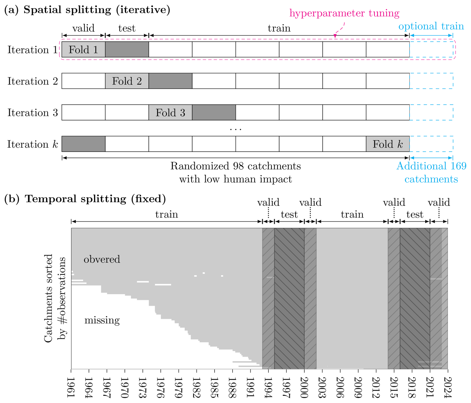
Figure 2 Cross-validation scheme: panel (a) shows the spatial domain, consisting of 98 catchments in Switzerland, which we randomly divided into k=8 sets. These sets were used iteratively, allowing each to serve once as a validation set and test set. Catchments significantly affected by human actions were optionally included in the training phase to enrich model learning, but they were consistently excluded from the validation and test phases to maintain the focus on natural runoff patterns. In panel (b), the time domain is delineated into fixed training, validation, and test periods. The used sets are the intersections of these spatiotemporal splits. With the initial iteration, hyperparameter (HP) tuning was performed, and the best HPs identified were then applied in subsequent cross-validation steps. By evaluating the model on the test sets, we comprehensively assessed the model's skill in generalizing across both spatial and temporal dimensions.

In each of the k iterations, six catchment sets were used for training, i.e., for optimizing the neural network parameters, while one set was used for validation and one for testing. After an epoch, i.e., one full iteration through the training data, the loss was computed on the validation set. The loss was monitored and training was interrupted if the loss on the validation set increased over a given number of epochs (the “patience”). The best model in terms of the validation loss was then restored and used for prediction on the test set. This routine is called “early stopping” and reduces overfitting (Yao et al., 2007). The final predictions on the test set were then used for model evaluation. As each catchment set was the test set once, we obtained independent test predictions for each of the 98 catchments.

3.5 Factorial experiment and model evaluation

In this section, we describe the model setups tested in a factorial experiment and the model evaluation procedures. We selected the best-performing model based on the median Nash–Sutcliffe modeling efficiency (NSE, Nash and Sutcliffe, 1970) across catchments, evaluated on the test set. The NSE as defined in Eq. (13) is calculated at the catchment level:

$$\begin{array}{}\text{(13)}& {\displaystyle }{\displaystyle }\text{NSE}=\mathrm{1}-{\displaystyle \frac{{\sum }_{t=\mathrm{1}}^T{\left(y_t-{\widehat{y}}_t\right)}^{\mathrm{2}}}{{\sum }_{t=\mathrm{1}}^T{\left(y_t-\stackrel{\mathrm{‾}}{y}\right)}^{\mathrm{2}}}},\end{array}$$

where y_t is the observed runoff and ${\widehat{y}}_t$ is the simulated runoff at time t of T total time steps. $\stackrel{\mathrm{‾}}{y}$ is the mean of the observed time series. The NSE can take values from −∞ to 1, where values above 0 indicate that the predictions are better than taking the mean of the observations and 1 means perfect prediction. Note that the NSE is closely related to R², but the NSE normalizes the sum of the squared residuals using the catchment variance instead of the global variance. Hence, the NSE does not place more emphasis on catchments with larger variance and is, therefore, also sensitive to catchments with a low dynamic range.

Different model setups were tested in a factorial experiment, and each combination of the factors was evaluated. The first factor determines the temporal component of the overarching model architecture: {LSTM,TCN}. The next factor determines whether the target variable and predictions are transformed using the square root, in order to reduce the skewness of the distribution: {T_none,T_sqrt}. We tested the inclusion of the 169 optional catchments (267 in total with the 98 default catchments) in the training set, compared to the 98 only (Fig. 2a): {C₉₈,C₂₆₇}. The last factor concerns the usage of static input variables. Due to the relatively large number of catchment properties (28), we alternatively used dimensionality-reduced static features. Using principal component analysis (PCA, Wold et al., 1987), all static features except catchment area were compressed into five components, which represent 66 % of the variance. Catchment area was always treated as a separate static input, as we consider it to be a key input feature. Hence, we either use catchment area only, a dimensionality-reduced version of the static variables using PCA, or all static variables described in the data section: $\mathit{\{}{S}_{\text{area}},S_{\text{PCA}},S_{\text{all}}\mathit{\}}$.

This yields a total of 24 models, and for each of them independent hyperparameter tuning and cross-validation were performed. Note that the fusion strategy for static and dynamic features, introduced in Sect. 3.1, was not considered a factor here but was part of the hyperparameter tuning.

To better understand the error structure, we also evaluate the MSE decomposition into bias, variance, and phase error (Kobayashi and Salam, 2000; Gupta et al., 2009):

$$\begin{array}{}\text{(14)}& {\displaystyle }{\displaystyle }{e}_{\text{MSE}}=\stackrel{e_{\text{bias}}}{\overbrace{({\mathit{\mu }}_{\widehat{y}}-{\mathit{\mu }}_y{)}^{\mathrm{2}}}}+\stackrel{e_{\text{variance}}}{\overbrace{({\mathit{\sigma }}_{\widehat{y}}-{\mathit{\sigma }}_y{)}^{\mathrm{2}}}}+\stackrel{e_{\text{phase}}}{\overbrace{\mathrm{2}{\mathit{\sigma }}_{\widehat{y}}{\mathit{\sigma }}_y(\mathrm{1}-r)}},\end{array}$$

where μ is the mean and σ is the standard deviation of the simulations $\widehat{y}$ and the observations y, and r is the linear correlation coefficient between them. The squared bias e_bias reflects the model fit in terms of the average and the variance error e_variance in terms of the scale. The phase error e_phase measures the reproduction of the timing, i.e., how well the dynamics are matched regardless of bias and scale.

3.6 Runoff reconstruction

To achieve a complete contiguous reconstruction from 1962 to 2023 for the small- to medium-sized catchments with national coverage (Fig. 1), we used the best-performing model from the cross-validation. The best model was selected based on median test set NSE across catchments. From the ensemble members from the 8-fold cross-validation, we obtained eight reconstructions with full coverage, of which we use the median (average of the two middle values) as the final data product. The year 1961 was removed from the reconstruction as it served as spinup.

4 Results

4.1 Catchment-level performance and benchmarking

In this section, we evaluate the model performance at the catchment level and compare the data-driven models. All the analyses are, unless stated otherwise, based on the test set (Fig. 2), i.e., spatially and temporally distinct data. Due to the iteration over the catchment groups in the cross-validation, each catchment was in the test set once. The fixed splitting of the time domain, however, restricts our evaluation to the test periods, i.e., January 1995–December 1999 and January 2016–December 2020. Throughout the evaluation, we use the hydrological model PREVAH as a benchmark.

4.1.1 Model performance

To understand the capabilities of our model to represent daily runoff at the catchment level, we evaluate the model performance first. Figure 3 presents the empirical cumulative density functions for different metrics across the 98 catchments. Models based on the TCN architecture are depicted in blue, those using LSTM networks in red, and the PREVAH model in black. The model with the best performance is emphasized using a thicker line. Figure 3a focuses on the NSE, while Fig. 3b–d provide a detailed breakdown of the MSE into its components – squared bias, variance error, and phase error – as introduced previously.

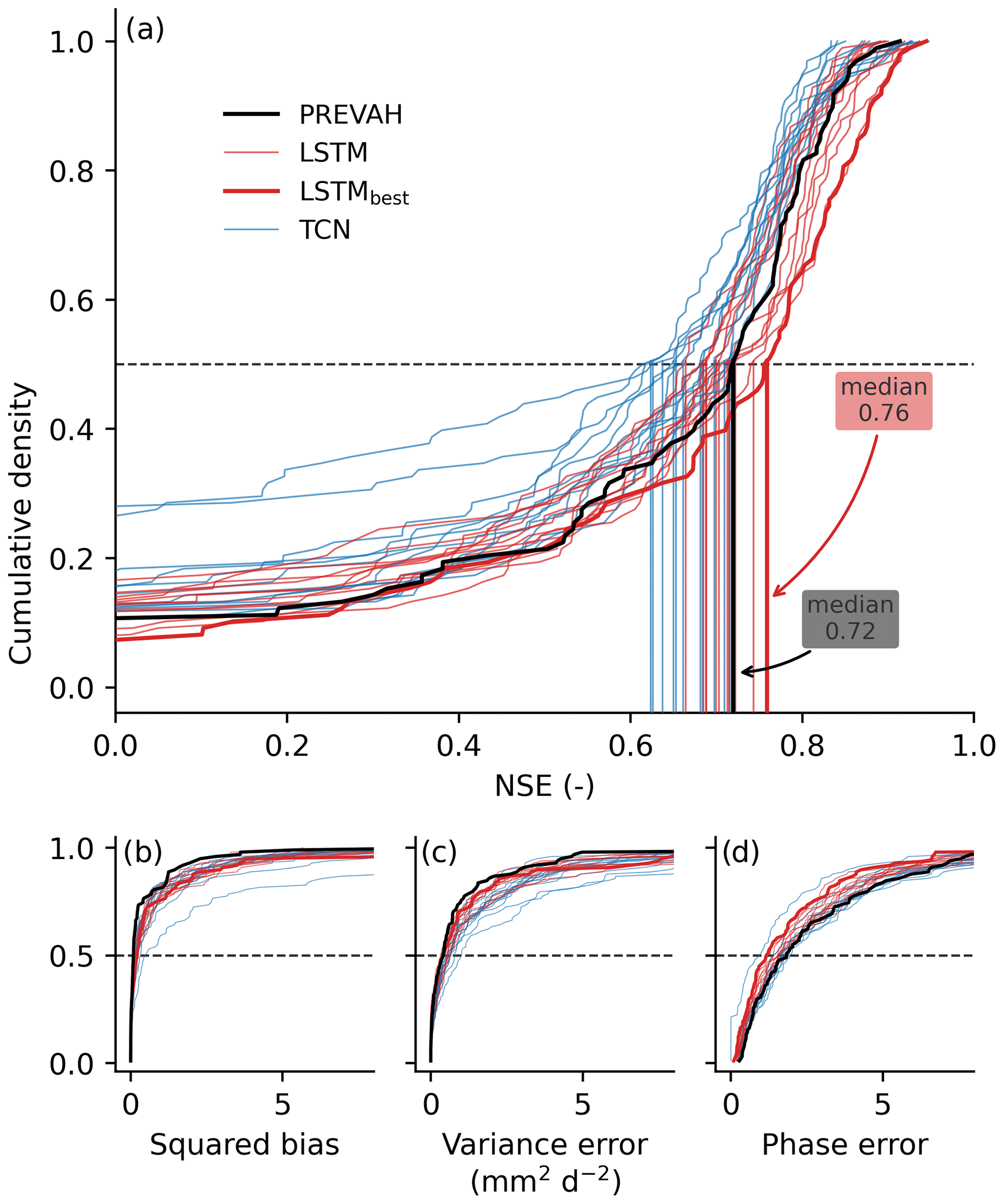
Figure 3 The catchment-level model performance across the 98 catchments evaluated on the test set that was not used for model calibration. We show different versions of the data-driven models, corresponding to the model setups: blue represents the convolution-based architectures (TCN) and red the LSTM architectures. The PREVAH model (black solid line) serves as a benchmark. The best-performing model (LSTM_best), used for the reconstruction, is highlighted. The y axis represents the cumulative probability density, i.e., the fraction of catchments that have the given value or lower. Panel (a) shows the Nash–Sutcliffe modeling efficiency (NSE), with median values as the vertical lines. Panels (b)–(d) show the squared bias, variance error, and phase error, respectively. Note that here, other than for the NSE in panel (a), lower values are better. The x axes are truncated.

Overall, we observed a large variance in performance across the model setups in terms of catchment-level NSE, and the TCN-based models performed worse than the LSTM model in general. This is mainly due to the two best-performing LSTM models (see also the model NSE in Appendix A, Tables A2 and A3). The best-performing LSTM (LSTM_best) achieved a median NSE of 0.76. The MSE decomposition shown in Fig. 3b–d indicates that LSTM_best (thick red line) is among the best models in terms of all error components. The phase error contributed most to the overall error by a wide margin, signifying that representing the timing of the runoff is more challenging than representing the average and the scale.

The best-performing setup was $\mathit{\{}\text{LSTM},S_{\text{all}},C_{\mathrm{267}},T_{\text{sqrt}}\mathit{\}}$, i.e., with all the static features, additional training catchments, and square root transform of the target, paired with the LSTM architecture. This model performed only marginally better than $\mathit{\{}\text{LSTM},S_{\text{all}},C_{\mathrm{98}},T_{\text{sqrt}}\mathit{\}}$, i.e., the one not using the additional catchments for training. These models both worked best with the pre-fusion with encoding approach (see Sect. 3.1). An overview of all the model setups and their performance is provided in Appendix A1, and a short discussion of the factorial experiment can be found in Appendix A2.

The PREVAH model achieved a median NSE of 0.72 (Fig. 3a), which is marginally lower than LSTM_best (NSE of 0.76) yet better than some of the other data-driven models. The PREVAH model showed a similar bias and variance error (Fig. 3b–d) to those of LSTM_best in terms of the median, yet it seems to be more robust in representing these aspects, as LSTM_best lags behind in the larger errors. Regarding the phase error, in contrast, the data-driven models in general and LSTM_best in particular clearly outperformed PREVAH across the catchments.

Next, we investigate the spatial distribution of the errors. First, we notice that the performance of LSTM_best in terms of NSE, shown in the top-left panel of Fig. 4, does not exhibit a clear spatial pattern. However, the model seems to struggle with some particular catchments. Interestingly, these are the very catchments where PREVAH clearly outperformed LSTM_best (compare the Fig. 4 top-left-panel dark-blue values to its lower-left-panel dark-red values).

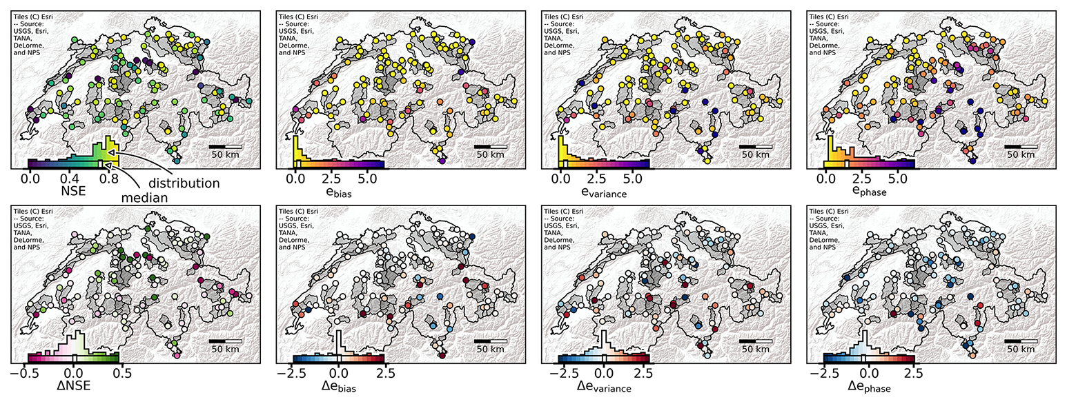
Figure 4 Spatial catchment-level performance of our best-performing model (LSTM_best) contrasted with the PREVAH model. The top row shows the performance of LSTM_best, with the NSE in the leftmost panel and the bias (e_bias), variance error (e_variance), and phase error (e_phase) in the remaining panels. Note that, in the top row, yellowish colors indicate better performance; i.e., for NSE, a larger number is better, and for the error components lower numbers are preferred. The bottom row shows the performance difference between LSTM_best and PREVAH. Here, reddish colors indicate that PREVAH performs better than LSTM_best, i.e., negative values for the NSE and positive values for the error components. The inset histograms represent the distribution of the catchment metrics, and the white bar indicates the median of the distribution per panel. The evaluation is performed on the test set, but all the catchments are in this set once in our cross-validation setup.

To understand how these spatial patterns are linked to catchment properties, we performed an exploratory analysis. First, we identified the tails of the distributions (inset histograms in Fig. 4 and PREVAH performance – not shown) using the 10th and 90th percentiles. We then compared properties of catchments in the tails to the “normal” group (between the 10th and 90th percentiles) using the two-sided, nonparametric Mann–Whitney U test with a significance level of α=0.1 (Mann and Whitney, 1947). The analysis was restricted to a subset of catchment properties: mean and variance of runoff, elevation, catchment area, and water body fraction. Here, we report the most notable findings of this ad hoc analysis.

For LSTM_best, poor performance (NSE below 0.14) was observed in catchments with a low mean and runoff variance, whereas good performance (NSE above 0.86) was achieved in catchments with a high runoff variance. Similarly, PREVAH struggled (NSE below 0.08) in catchments with a low runoff mean and variance as well as under low-elevation, lake-dominated conditions, but it performed well (NSE above 0.84) in catchments with a high runoff mean, a large catchment area, and minimal lake presence. As expected, the bias of LSTM_best was low in catchments with a low runoff mean and variance, with variance error increasing under high-runoff-variance conditions. The phase error for LSTM_best was lowest in catchments with a low runoff mean and variance and a large catchment area.

Significant differences in NSE performance were observed between the two models in catchments with low runoff variance. PREVAH outperformed LSTM_best (NSE improvement above 0.28) in catchments with both low runoff mean and variance. Conversely, LSTM_best clearly outperformed PREVAH (NSE improvement above 0.28) in low-elevation, lake-dominated catchments that also had low runoff variance.

4.1.2 Annual variability and trends

For a reconstruction product, it is crucial to adequately represent yearly variability and long-term trends. We, therefore, evaluate this aspect on annual runoff aggregates (Fig. 5). The best-performing model, LSTM_best, represented the interannual variability (Fig. 5a), quantified as the Pearson correlation coefficient between the annual values for each catchment, well, with a median of r=0.93 and 75 % of the catchments above r=0.85. The bias averages close to zero, and for 50 % of the catchments it was in the range −250–250 mm yr⁻¹ (Fig. 5b). On the interannual variability, PREVAH showed a slightly lower correlation (Fig. 5a) across the catchments, with a median of r=0.91. In terms of bias, PREVAH performed marginally better, with a median closer to zero and a lower spread (Fig. 5b).

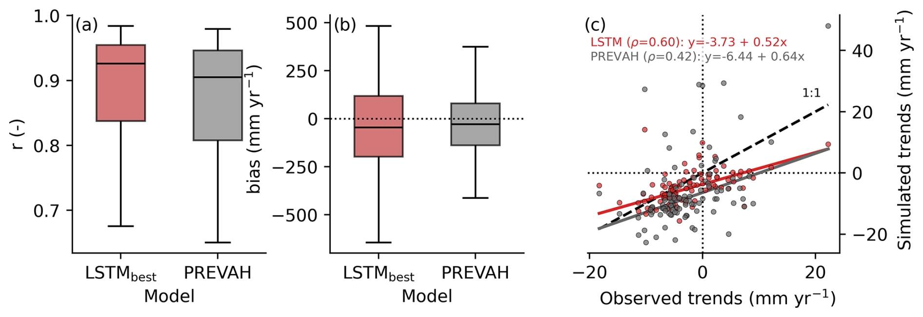
Figure 5 Catchment-level evaluation at the annual scale. (a) The Pearson correlation (r) and (b) bias (mm yr⁻¹) distribution across 98 training catchments evaluated on the test set. (c) The simulated annual runoff trends compared to the observations. The points represent the linear trend (found by the robust least-squares fit) of the individual catchments. Note that, for the trend calculation, the time range from 1995 (start of the first test period) to 2020 (end of the second test period) was used. The inset equation shows the linear least-squares fit and the corresponding rank correlations.

Figure 5c illustrates how the models captured spatial patterns of annual trends between January 1995 and December 2020 (Fig. 5c). The agreement was calculated independently by first computing the catchment-level linear trends for the observations and simulations using PREVAH and LSTM_best with the robust Theil–Sen estimator (Sen, 1968). Then, we fit a regression between the observed and estimated trend slopes of the two models using robust regression with Huber weighting and the default tuning constant of c=1.345 (Huber and Ronchetti, 2009). This approach reduced the impact of outliers by giving lower weight to large residuals. To quantify the alignment of the simulated trends, we used the Spearman correlation (ρ), which is relatively robust against outliers. While LSTM_best represented the spatial patterns of the linear trend relatively well with a correlation of ρ=0.60, PREVAH achieved a correlation of ρ=0.42. Both models underestimated the strength of negative and positive trends, with slopes of 0.52 (LSTM_best) and 0.64 (PREVAH), and they exhibited small negative biases of −3.73mm yr⁻¹ (LSTM_best) and −6.44mm yr⁻¹ (PREVAH).

4.2 Qualitative evaluation of selected catchments

To understand how the models represent different hydrological regimes, we performed a qualitative comparison for a selection of catchments. For this purpose we selected single catchments that are dominated by (a) rainfall, (b) lakes, (c) snow, or (d) glaciers (Fig. 6). These example catchments serve as means for qualitative model comparison, and we do not expect these insights to directly generalize across catchments.

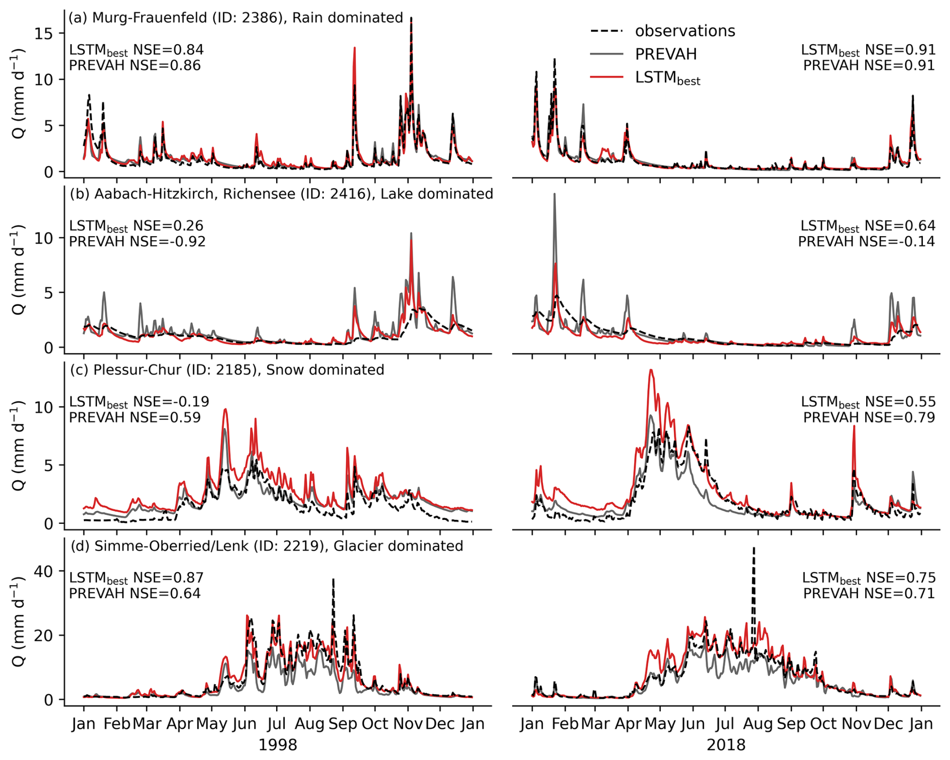
Figure 6 Daily runoff Q (mm d⁻¹) for four selected catchments and 2 distinct years selected from the test periods. Observations (dashed black line), PREVAH simulations (grey), and out-of-catchment predictions of the data-driven LSTM_best (red) are shown. The catchments were selected to represent different modeling challenges: (a) rainfall-, (b) lake-, (c) snow-, and (d) glacier-dominated. The inset NSE values represent the model performance for the selected year.

The rainfall-dominated catchment, the Murg at Frauenfeld (ID 2386), is located in the northwest of Switzerland on the Swiss Plateau, with an area of ∼200 km² and an average elevation of ∼600 m. The maximum snow water equivalent (SWE) has been below 80 mm in recent years (Höge et al., 2023) and was not considered to affect runoff for most days of the year. The lake-dominated catchment, the Aabach at Hitzkirch (ID 2416), is located in the central Pre-Alps, with an area of ∼70 km² and an average elevation of ∼600 m. The gauging station is located just a few hundred meters from the outflow of the ∼5 km² Lake Baldegg, which damps runoff peaks and also affects the low-flow regime. The snow-dominated catchment, the Plessur at Chur (ID 2185), is located in the eastern Swiss Alps, with an area of ∼250 km² and an average elevation of ∼1900 m (from ∼500 to ∼3000 m). The maximum SWE varied in the past 25 years between 200 and 500 mm. There are no large glaciers in this area that could influence runoff. The glacier-dominated catchment, the Simme at Oberried/Lenk (ID 2219), is located in the western Swiss Alps, with an area of 35 km² and an average elevation of ∼2300 m (from ∼1000 to ∼3200 m). More than 25 % of the area is covered by glaciers. The maximum SWE varied in the past 25 years between 400 and 1100 mm.

For the rainfall-dominated catchment, PREVAH and LSTM_best showed similar behavior (Fig. 6a), and both models were able to reproduce the runoff peaks and overall patterns. For the lake-dominated catchment, LSTM_best outperformed the PREVAH model in terms of NSE (Fig. 6b). Visual inspection shows high peaks in PREVAH simulations, which indicate missing buffering dynamics in lakes. This is not surprising, as PREVAH does not represent lakes explicitly, while the LSTM model can learn the buffering implicitly via the catchment properties, of which the fraction of water bodies may be the most relevant. For the snow-dominated catchment shown in Fig. 6c, the PREVAH model managed to represent the runoff processes better in 1998 and similarly in 2018. Here, LSTM_best overestimates runoff in general, and it peaks particularly in summer. Snowmelt responds strongly to radiation, which was not included as a driver of the LSTM model. Further, snow-related processes are spatially heterogeneous, depending on elevation and aspect. The lumped LSTM model cannot resolve these processes at the subcatchment level, while the PREVAH model operates on a high-resolution grid. Although worse in terms of NSE, the LSTM model managed to better represent the snowmelt in 2018, possibly because snow had already melted away in the PREVAH simulation. In a glacier-dominated catchment, finally, LSTM_best represented the runoff patterns slightly better than PREVAH.

4.3 Runoff reconstruction

The reconstruction of daily runoff from 1962 to 2023, referred to as CH-RUN, was conducted with the best-performing model based on prior analysis. The final estimate was calculated as the median across the eight ensemble members from the cross-validation. Figure 7 shows the annual runoff as quantiles relative to the reference period from 1971 to 2000. The quantiles were calculated per catchment by comparing the annual values to the empirical distribution of the reference period. Turquoise colors indicate that, for a given catchment, the yearly average runoff is rather high compared to the reference, and brown colors signify dry years.

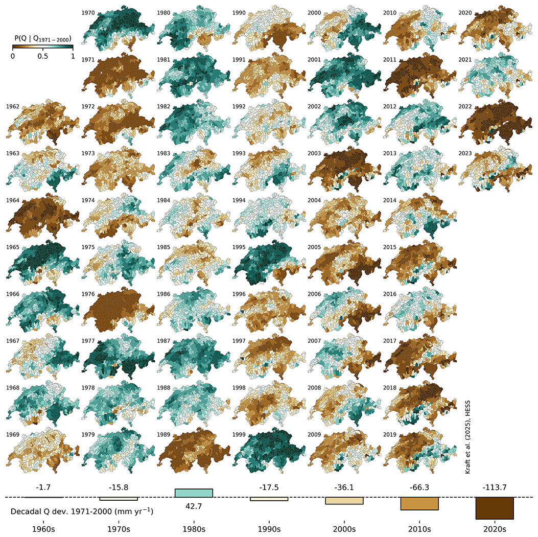
Figure 7 Spatially contiguous reconstruction of runoff from 1962 to 2023 from the CH-RUN reconstruction. The maps represent the yearly catchment-level runoff quantiles relative to the reference period (1971 to 2000) empirical distribution. The bottom bars show the decadal deviation (mm yr⁻¹) of the national-level runoff relative to the reference period (1971 to 2000).

The reconstruction suggests that dry years with similar intensities compared to the conditions of the 21st century were already present in the 1960s and 1970s (e.g., in 1964 and 1976). However, the frequency of dry years increased significantly – and that of wet years decreased substantially – according to the model estimates.

Figure 8 shows the annual national runoff anomalies and the corresponding trends for CH-RUN. According to the CH-RUN reconstruction, the recent dry conditions are matched by values in the 1960s and 1970s in terms of amplitude, while the frequency of dry years increased and that of wet years decreased. Extremely dry years (exceeding the 0.1 quantile of the reference period) were absent in the 1980s and 1990s, while wet years (exceeding the 0.9 quantile of the reference period) were more frequent during this period. The last extremely wet year was 1999, and the driest year was 2022.

Figure 8 Annual runoff anomalies for Switzerland from 1962 to 2023 from the CH-RUN reconstruction. The bars represent the CH-RUN annual deviation (mm yr⁻¹) of the national-level runoff relative to the reference period (1971 to 2000). The aggregation from the catchment to the national level was done with the area-weighted mean. Positive anomalies are depicted in turquoise and negative ones in brown. The solid red line represents the trend, i.e., the low-pass-filtered signal using a Gaussian filter with a standard deviation of σ=2. The dashed lines are the 0.1 and 0.9 quantiles of the reference period.

In Fig. 9, the decadal mean values are disaggregated into seasonal patterns. Here, the average annual sums across the decades are shown, again relative to the reference period from 1971 to 2000. The decadal means again hint at strong trends towards less runoff on a yearly scale. In the winter months December to February (DJF), we see a slight tendency towards less runoff north of the Alps, while the 2020s exhibit more runoff in the Pre-Alps. From March to May (MAM), northern Switzerland, the Pre-Alps, and the canton of Ticino show a clear trend towards drier conditions. Even more pronounced, the June–August (JJA) period reveals a tendency towards less runoff in the central Alps with higher altitudes and the canton of Ticino. From September to November (SON), the patterns are again less distinct, yet there is a general trend towards drier conditions in most of the catchments.

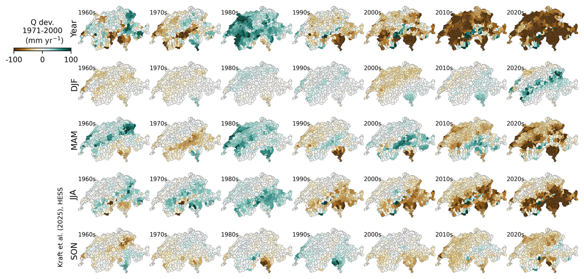
Figure 9 Decadal evolution of the spatially contiguous reconstruction of runoff from 1962 to 2022 by season from the CH-RUN reconstruction. The maps represent the decadal-average catchment-level runoff (mm yr⁻¹) relative to the reference period (1971 to 2000). From the top to bottom rows: year – full year; DJF – December to February; MAM – March to May; JJA – June to August; SON – September to November.

5 Discussion

5.1 Neural network architectures and the role of data

The better performance of the LSTM model compared to the TCN (Fig. 3) is somewhat surprising, as the latter has been reported to perform well in time series prediction settings (e.g., Zhao et al., 2019; Catling and Wolff, 2020; Yan et al., 2020). The difference in performance can be traced back to the two best-performing LSTM models (Fig. 3 and Tables A2 and A3) and hints at better capabilities of the LSTM model to represent interactions between meteorological and static features under these data-limited conditions. It seems that the LSTM model is more data-efficient than the TCN, which is also supported by the lower number of tunable parameters used by the former (see Tables A2 and A3). It might, therefore, be possible for the TCN to compete with the LSTM architecture if more training data are available. Other deep-learning approaches to modeling time series exist, of which transformer-based architectures (Vaswani et al., 2017) have become popular recently (Lim et al., 2021; Zhou et al., 2021; Xu et al., 2023). Due to the powerful and complex encoder–decoder structure, these models especially release their potential in forecasting settings and with large amounts of training data. Given the relatively low amounts of training data available for the study domain, we do not expect significant improvement from using such architectures. Nevertheless, exploration of this architecture may hold potential for improved reconstruction in the future.

In runoff modeling, integrating catchment properties with meteorological features is a prevalent approach (e.g., Kratzert et al., 2019). We found that the most effective data fusion method involved channeling static variables through the LSTM model's temporal layers while handling some nontemporal interactions in an upstream encoding layer. Our LSTM model successfully learned the complex interactions between static and meteorological features, extending its applicability to untrained catchments and time ranges. Enhancing the model's predictions was achieved by incorporating a broader range of catchments and fully utilizing catchment properties (Fig. A1), acknowledging that a wider input feature space necessitates more data. This finding aligns with our previous diagnosis of spatial information limitations due to the relatively small number of training catchments. Although the importance of data has been reported well (Kratzert et al., 2018; Gauch et al., 2021b), these results reaffirm the value of additional data in enhancing model performance. Consequently, we recommend exploring methods to incorporate more training data, such as transfer learning from other tasks (Sadler et al., 2022) or other regions (Pan and Yang, 2010; Yao et al., 2023; Xu et al., 2023), e.g., from large-scale datasets (Kratzert et al., 2023; do Nascimento et al., 2024), and considering alternative data sources like bottom-up data mobilization efforts (Do et al., 2018; Gudmundsson et al., 2018; Nardi et al., 2022; Kebede Mengistie et al., 2024) as promising avenues for future research.

It is encouraging to see that the LSTM model did manage to implicitly learn complex runoff dynamics across hydrological regimes (Fig. 6). The data-driven model has learned buffering effects by lakes and, to a certain extent, runoff-generating processes related to snow and, possibly, glaciers. Similar behavior has been reported before. Kratzert et al. (2019) and Lees et al. (2022), for example, reported that an LSTM model was able to represent long-term snow dynamics. We expect potential for improvement by better representing buffering processes via routing of the runoff (Bindas et al., 2024) and by an improved representation of snow and glacier processes. This can be achieved via the combination of physically based and data-driven modeling (Reichstein et al., 2019), e.g., by directly employing physical constraints in an end-to-end hybrid physics–machine learning setup (Kraft et al., 2022, 2020; Höge et al., 2022), by penalizing physically implausible simulations during training (Daw et al., 2021), or by regularizing the model with auxiliary tasks (Sadler et al., 2022).

5.2 Comparison with the PREVAH model

Although some neural networks outperformed the PREVAH model (Fig. 3), the differences in terms of NSE were small. The marginally better representation of runoff mean and amplitude by PREVAH makes sense intuitively, as the data-driven model has a very limited number of training catchments to learn spatial features from. Equivalently, the better representation of temporal patterns by the LSTM model could be explained by the fact that it has access to long time series to learn dynamics from. It is not surprising that machine learning can outperform physically based models in runoff prediction, as this has been demonstrated in previous studies (e.g., Kratzert et al., 2018; Lees et al., 2021; Gudmundsson and Seneviratne, 2015; Ghiggi et al., 2021). However, in this study, we used a limited number of meteorological drivers compared to the needs of the PREVAH model. Furthermore, PREVAH is an expert model that uses carefully regionalized parameters for the study domain (Viviroli et al., 2009c). As PREVAH provides the natural discharge within the catchment domain, it is not able to capture the dampening effect provided by lakes (Fig. 6b). The LSTM model is able to cope with such effects as part of its global calibration result.

From the analysis of the spatial patterns of the model performance (Fig. 4), we learned that LSTM_best encountered challenges with dry catchments that have both low runoff mean and variance. This was not surprising due to the high signal-to-noise ratio in runoff observations and the sensitivity to minor variability in the meteorological variables and catchment properties in dry catchments. Similarly, PREVAH struggled with dry conditions, but it still clearly performed better under such conditions. In contrast, LSTM_best represents lake-dominated catchments with low elevation significantly better. This was expected, as PREVAH does not represent lake processes, and therefore it cannot properly represent their dampening effect. The interaction with elevation could be explained by the fact that the largest lakes in Switzerland are at medium to low elevations.

The PREVAH model is already used successfully for reconstruction (Otero et al., 2023) and future (Laghari et al., 2018; Brunner et al., 2019b) climate scenarios. With the objective of real-time monitoring, long-term reconstruction, and potentially efficient simulation of climate scenarios in mind, we consider the similar performance compared to the benchmark to be sufficient. The similar ability to represent interannual patterns by LSTM_best and the slightly better fidelity of trends (Fig. 5) are, especially given the lowered data requirements, encouraging. We want, however, to state here upfront that a process-based hydrological model has advantages over a data-driven model, such as interpretability and physical consistency.

5.3 Plausibility of the runoff reconstruction product

The reconstruction of runoff back to the early 1960s for Switzerland is a novelty enabled by the reduced data needs of our deep-learning-based approach compared to the PREVAH model. Here, we evaluate the plausibility of the simulated patterns based on Figs. 7–9 by contrasting them with prior knowledge.

The overall trend towards drier conditions simulated by our data-driven model aligns with independent studies. This has been reported widely for Europe (Orth and Destouni, 2018; Hanel et al., 2018) and specifically for Switzerland (Hohmann et al., 2018; Brunner et al., 2019b; Henne et al., 2018). Interestingly, the results reveal that the runoff anomalies of the 2022 drought (e.g., Toreti et al., 2022; Schumacher et al., 2024) were larger than those of the well-documented 2003 drought (e.g., Ciais et al., 2005; Rebetez et al., 2006; Seneviratne et al., 2012). The identified drying trend in the summer season is consistent with a reported increase in agroecological droughts in western and central Europe in the latest report of the Intergovernmental Panel on Climate Change (IPCC; Arias et al., 2023) and may indicate the presence of a drying trend in streamflow in this region, which was assigned low confidence at the time of the IPCC report (Seneviratne et al., 2021).

In the winter months, an increase in runoff in the Pre-Alps may be linked to an earlier onset of snowmelt (Vorkauf et al., 2021). In the same region and other mid-altitude areas such as the Jura sub-Alpine mountain range, runoff decreases in spring. This could be related to a combination of a trend towards lower snowmelt due to less snowfall during winter (Matiu et al., 2021) and an earlier onset of snowmelt due to the previously mentioned warmer temperatures. The Alps are, supposedly, similarly affected by those effects, yet the onset of thawing is delayed due to higher altitudes, and hence we see the main contribution to negative trends in the later summer. In Ticino, a strong trend towards warmer temperatures has been reported, although precipitation seems not to show significant trends (Reinhard et al., 2005). The negative trend in summer is likely caused by both a lack of snowmelt and an increase in evapotranspiration via warmer air temperatures, which can have a significant impact on runoff (Teuling et al., 2013; Goulden and Bales, 2014).

5.4 Potential applications

Other than catchment-level observations, the spatially and temporally complete reconstruction provides a tool for studying runoff beyond the observational horizon and for ungauged catchments. The focus on catchments with low human impacts during model training allows the investigation of physical processes in isolation. This is an advantage for climate-focused studies, as it is challenging and often not possible to disentangle effects of human water use from physical effects associated with human-induced climate change. We encourage researchers to use the CH-RUN product for trend analysis and to understand the drivers of simulated patterns. We further see potential in using CH-RUN as an independent benchmark dataset for hydrological models: it is challenging to understand the different sources of uncertainty during model development. Having a methodologically independent benchmark dataset can help disentangle methodological and data limitations.

With our data-driven approach, we achieve a speedup by a factor of 600 compared to PREVAH, assuming PREVAH is run parallelized across 100 central processing units (CPUs) and CH-RUN is employed on a high-performance graphics processing unit (GPU). The reconstruction for the entire domain took approximately 20 s for one ensemble member on an NVIDIA A100 GPU. This speedup enables computationally cheap real-time monitoring of runoff on a national scale. In addition, the model can be fed with meteorological forecasts, which would enable early warning of floods and droughts. A common use case for hydrological models is to run scenarios, i.e., to simulate responses to a changing climate or to attribute runoff patterns to anthropogenic forcing. However, running scenarios with physically based models is computationally expensive, which limits the ensemble size and forecast horizon. The speedup compared to a traditional hydrological model allows thousands of scenarios to be run with ease. The application in early warning and running scenarios must be examined carefully and may require further calibration steps, but it holds potential for understanding and mitigating climate change impacts in the near future.

5.5 Limitations

In the evaluation at the catchment level, it was observed that the CH-RUN model, although effective in general, faces challenges under certain conditions in accurately representing runoff, such as in catchments with a low runoff mean and variance. The model's performance was evaluated in catchments with minimal human impact, such as dam operations and surface irrigation, in order to reduce anthropogenic influences on the results. However, the model did not incorporate detailed land use information beyond basic surface classifications, thereby not accounting for direct human alterations in the hydrological system.

A limitation of our approach was the reliance on air temperature and precipitation data only for long-term reconstruction, excluding other meteorological factors like sunshine hours, which can only be implicitly approximated by the model via the available input variables. The assumption of static variables, such as land use and glacier coverage, being constant over time is a necessary simplification but introduces potential inaccuracies. This is particularly critical as land use can vary, and glacier areas are known to decrease over time, potentially leading to biases, especially in the early stages of the reconstruction, when observational data are sparse.

Moreover, the dataset used for training the model and the dataset for reconstruction are not entirely independent, though they are not identical. The temporal overlap of the training set within the reconstruction period was unavoidable due to data limitations. Efforts were made to mitigate the risk of overfitting by employing a distinct validation set that was both spatially and temporally separated from the training data.

In runoff modeling, the quality of meteorological drivers has a high impact on model performance, and both meteorological products used here have known limitations. The TabsD product of air temperature shows a clear relationship between the error and number of stations used for the interpolation, which results in larger errors in the 1960s and 1970s that are most pronounced in the winter months, particularly in the Alps and Ticino. The linear trend (1961–2010) of interpolated air temperature shows relatively low agreement with the observed trends (Frei, 2014). The RhiresD precipitation product is affected by two primary sources of uncertainty: the rain gauge measurements are prone to undercatch, leading to underestimation of precipitation, particularly with heavy winds and snow in general (Neff, 1977). This leads, in Switzerland, to underestimations of about 4 % at low elevations and up to 40 % at high altitudes in winter (Sevruk, 1985). From the interpolation, there is a tendency to overestimate light precipitation and underestimate heavy precipitation (MeteoSwiss, 2021b), although these inaccuracies are reduced for areal aggregates such as the catchment averages deployed in the present study. Although no information on the accuracy over time was found, it is expected that the sparser measurement network in the 1960s and 1970s will lead to larger errors during this period, similar to the TabsD product. These uncertainties are expected to affect the results substantially. We acknowledge that, for the early reconstruction period (1960s and 1970s), where fewer measurement stations were available, the reconstruction may be less trustworthy. The low agreement of interpolated air temperature trends with observations could explain why both PREVAH and CH-RUN struggle to represent extreme runoff trends. While we did not specifically investigate the representation of extreme runoff events in this study, we expect that the overestimation of weak precipitation events and the underestimation of strong precipitation events will result in a bias in runoff simulations.

Finally, our deep-learning model depends heavily on the availability and diversity of data. Representing infrequent occurrences or events, which are less common in the data distribution, poses a significant challenge. Consequently, the model's ability to accurately depict rare and extreme hydrological events, such as sudden heavy rains leading to flash floods, is likely limited. This aspect is underscored by the inherent difficulties in modeling the “long tail” of event distributions (Zhang et al., 2023).

6 Conclusions

In this study, we developed a data-driven daily runoff reconstruction product for Switzerland, spanning the period from 1962 to 2023. Our model not only matched but also surpassed the performance of an operational hydrological model at the catchment level. This achievement is particularly noteworthy considering the reduced data requirements, a limitation necessary to achieving such an extensive reconstruction period. Our model effectively captured daily runoff patterns and interannual variability and represents long-term trends decently, providing a comprehensive and satisfying depiction of runoff dynamics.

The reconstruction product revealed interesting patterns in long-term runoff trends that align with prior knowledge. The additional reconstruction of the 1960s and 1970s suggests that the negative decadal runoff trend is driven by an increase in the frequency, rather than amplitude, of dry years, along with a decrease in the frequency of wet years. We diagnosed a trend towards lower runoff at the national scale that was mainly linked to the summer months, where the spatial patterns of runoff indicated increasingly dry conditions, particularly at mid to high altitudes. We encourage in-depth investigation of the identified patterns in subsequent studies.

One of the major strengths of our approach lies in its computational efficiency, which opens up possibilities for contiguous near-real-time monitoring and potential forecasting of runoff. The reduced data demands of our model make it an invaluable tool for scenario simulation and attribution of trends to anthropogenic climate change, allowing for rapid evaluation of thousands of scenarios that was not feasible with traditional physically based models.

Looking ahead, we believe that the current approach could be enhanced further by integrating additional data constraints or incorporating physical knowledge. Specifically, for a more accurate representation of large catchments, we see the inclusion of routing processes as a vital next step.

Appendix A: Model training

A1 Hyperparameter tuning

The hyperparameter space searched is shown in Table A1. model_dim denotes the model dimensionality, i.e., the size of the internal representations. enc_dropout refers to the dropout (random deactivation of nodes with probability p during training) applied in the encoding layers, and fusion_method refers to the method used for fusion of the temporal and static variables. For the AdamW optimizer, learning_rate denotes the step size and weight_decay the L2 regularization. temp_layers refers to the number of stacked temporal layers for both the LSTM model and the TCN, and kernel_size is the dimensionality of the 1D kernel used for convolution in the time dimension for the latter. An optional temporal_dropout is used for the TCN. The performance of the models and the corresponding hyperparameters is provided in Table A2 for the LSTM models and in Table A3 for the TCNs.

Table A1 The search space for hyperparameter tuning. The common hyperparameters were used for both architectures, and the other ones are model-specific.

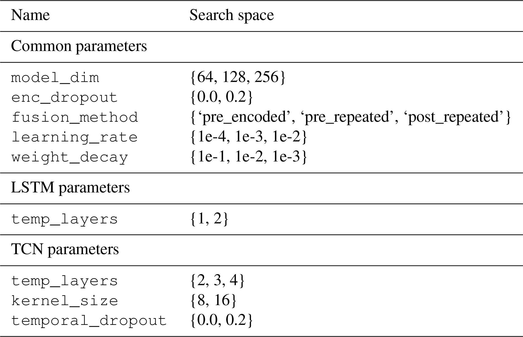
model_dim corresponds to the model dimensionality, which is shared among all feed-forward and temporal neural networks. enc_dropout was used in the encoder layers prior to the temporal layer, and fusion_method corresponds to the approaches described in Sect. 3.1. learning_rate and weight_decay are parameters of the optimizer and control the weight update step size and regularization, respectively. For the long short-term memory (LSTM) model and the temporal convolutional network (TCN), temp_layers defines the number of stacked temporal layers. For the latter, kernel_size is the width of the 1D convolution kernel applied along the time dimension, and temporal_dropout deactivates entire channels of input encoding instead of randomly dropping activations.

Table A2 Hyperparameters found by tuning for the LSTM-based architectures. The rows are sorted by the catchment-level Nash–Sutcliffe modeling efficiency (NSE) in descending order, and the rank column represents the overall rank among all the models. The columns allbasins (using additional catchments for training or not), sqrttrans (transform runoff with a square root or not), and static (use all static variables, a dimensionality-reduced version, or just the catchment area) refer to the factorial experiments described in Sect. 3.5. Columns model_dim, enc_dropout, fusion_method, temp_layers, learning_rate, and weight_decay denote the hyperparameters of the model. Column num_params shows the number of tunable model weights.

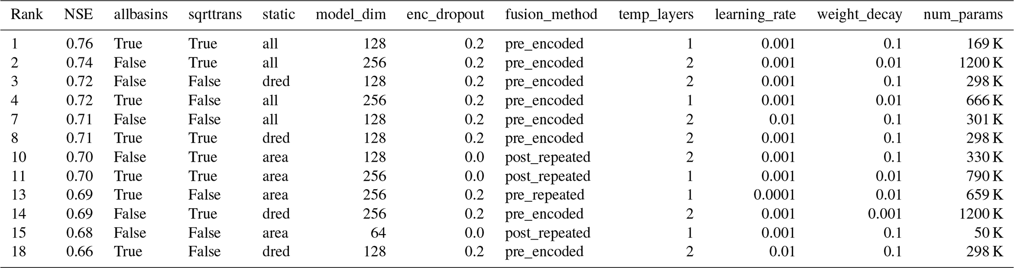
Table A3 Hyperparameters found by tuning for the TCN-based architectures. The rows are sorted by the catchment-level NSE in descending order, and the rank column represents the overall rank among all the models. The columns allbasins (use additional catchments for training or not), sqrttrans (transform runoff with a square root or not), and static (use all static variables, a dimensionality-reduced version, or just catchment area) refer to the factorial experiments described in Sect. 3.5. Columns model_dim, enc_dropout, fusion_method, temp_layers, kernel_size, learning_rate, and weight_decay denote the hyperparameters of the model. Column num_params shows the number of tunable model weights.

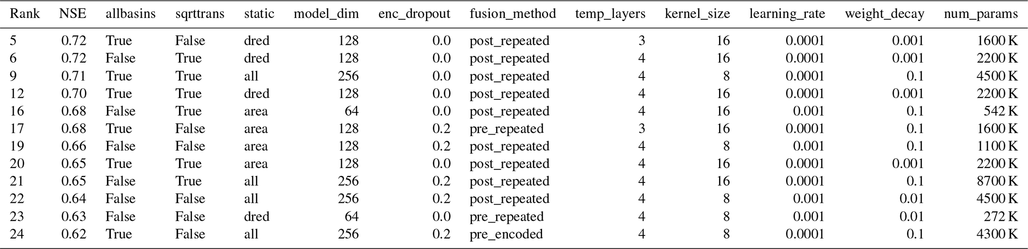
From the fusion methods introduced in Sect. 3.1, pre-fusion with encoding was selected most often for the LSTM architecture, while post-fusion was more commonly selected for the TCN (Appendix A, Tables A2 and A3). Note that the fusion was part of the hyperparameter tuning, and only the best approach is used to make the final predictions. For both architectures, pre-fusion with encoding was commonly selected if all the static variables were used as input. Interestingly, as seen in Tables A2 and A3, the number of tunable parameters, an outcome of the hyperparameter tuning process, was larger by a factor of 5 for the TCN architectures (2.8 million on average) compared to the LSTM models (0.52 million on average).

A2 Comparison of model setups

Here, we evaluate the factorial experiment outlined in Sect. 3.5. In Fig. A1, the diagonal shows how the model setups impact the median NSE across the catchments, and the offset triangle shows the interactions of the factors.

For the LSTM architecture, using all the training catchments and all the static variables had a higher impact on the outcome than the square root transform of the target variable, which was negligible. The factors “training catchments” and “static variables” interacted strongly, indicating that having both more training data and more information on catchment properties contributes more to the model performance than using the factors independently. The interaction with the “target transform”, in contrast, was minimal for the LSTM architectures. For the TCNs, the results look different. Using more static variables as input seems to have improved the model performance, while using additional training catchments did so only marginally and the interactions of the training catchments and static variables were less clear. Overall, the TCNs show a lower range of performance across the setups than the LSTM models.

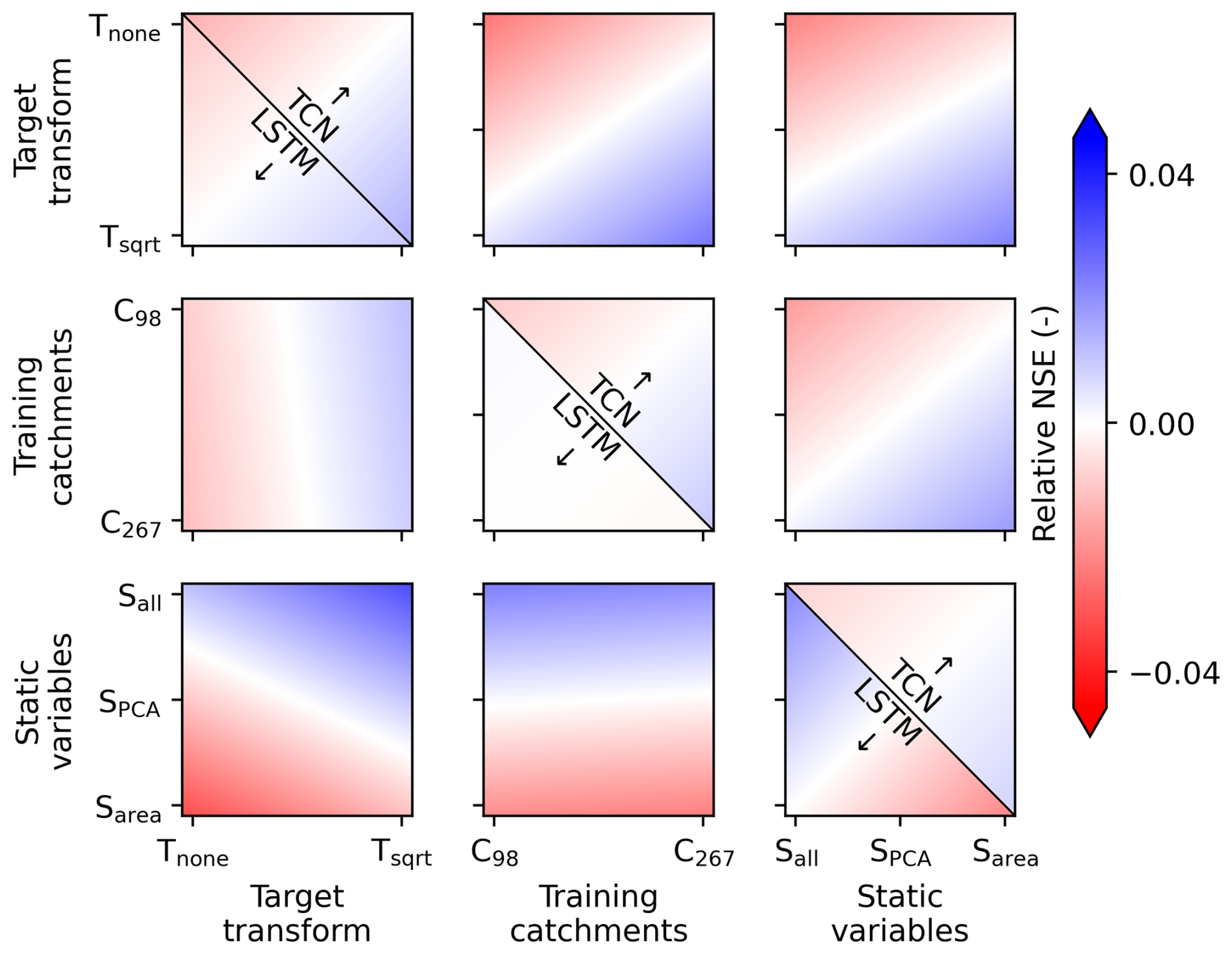
Figure A1 Model setup impact on performance and its interactions based on the median catchment NSE, evaluated on the spatially and temporally independent test set. The colors represent the NSE relative to the respective model mean across the setups: red represents worse performance, and blue represents better performance. The background gradients have been calculated using linear least-squares regression, with the model performance as the dependent variable. The offset lower triangular panels show results for the LSTM model, the offset upper triangular panels those for the TCN (i.e., variable interactions), and the three panels on the diagonal the main effects, split to distinguish between the two models. The x and y axes represent the setups tested in the factorial experiment. “Training catchments” refers to the catchments used for training: a subset of 98 catchments less impacted by anthropogenic factors (C₉₈) or all the catchments (C₂₆₇). “Target transform” is either T_none if the target variable was not transformed or T_sqrt for square root transform. “Static variables” is S_all if all the static variables are used, S_PCA if they are first transformed using PCA, or S_area if only the catchment area is used beyond the meteorological variables.