the Creative Commons Attribution 4.0 License.
the Creative Commons Attribution 4.0 License.
 | 27 Feb 2024
Toward interpretable LSTM-based modeling of hydrological systems
Luis Andres De la Fuente
Mohammad Reza Ehsani
Hoshin Vijai Gupta
Laura Elizabeth Condon
Several studies have demonstrated the ability of long short-term memory (LSTM) machine-learning-based modeling to outperform traditional spatially lumped process-based modeling approaches for streamflow prediction. However, due mainly to the structural complexity of the LSTM network (which includes gating operations and sequential processing of the data), difficulties can arise when interpreting the internal processes and weights in the model.
Here, we propose and test a modification of LSTM architecture that is calibrated in a manner that is analogous to a hydrological system. Our architecture, called “HydroLSTM”, simulates the sequential updating of the Markovian storage while the gating operation has access to historical information. Specifically, we modify how data are fed to the new representation to facilitate simultaneous access to past lagged inputs and consolidated information, which explicitly acknowledges the importance of trends and patterns in the data.
We compare the performance of the HydroLSTM and LSTM architectures using data from 10 hydro-climatically varied catchments. We further examine how the new architecture exploits the information in lagged inputs, for 588 catchments across the USA. The HydroLSTM-based models require fewer cell states to obtain similar performance to their LSTM-based counterparts. Further, the weight patterns associated with lagged input variables are interpretable and consistent with regional hydroclimatic characteristics (snowmelt-dominated, recent rainfall-dominated, and historical rainfall-dominated). These findings illustrate how the hydrological interpretability of LSTM-based models can be enhanced by appropriate architectural modifications that are physically and conceptually consistent with our understanding of the system.
- Article
(10404 KB) - Full-text XML
-
Supplement
(7792 KB) - BibTeX
- EndNote


Scientific research that incorporates machine learning (ML) has exploded over the past several years, and hydrology is not an exception. Reasons for this include the existence of open-source application programming interfaces (APIs), the availability of large dataset repositories, and the ability to obtain good performance without requiring too much computational power (Hey et al., 2020; Pugliese et al., 2021). However, understanding (in a hydrological context) what is happening inside such models continues to limit the interpretability of their results (Xu and Liang, 2021).
Reasons for this lack of interpretability are diverse, but one of the most fundamental reasons is that many of the ML architectures have been developed to address problems that are, in many respects, quite different from the ones relevant to hydrology and/or the earth sciences. Specifically, many were developed in the general field of data science with a particular focus on classification or predictive performance, rather than on knowledge extraction.
By contrast, the scientific method typically presumes some degree of “interpretability and understanding” in the formulation of hypotheses and experiments. Using ML-based approaches for hypothesis testing can be challenging if we are unable to interpret what is happening inside the model or what is learned by our representations and how they are related to our scientific questions. This aligns perfectly when we check the definition of interpretability, “degree to which an observer can understand the cause of a decision” (Miller, 2019), which is fundamental if we want to learn from the analysis of data.
1.1 Lack of LSTM interpretability
In hydrology, the long short-term memory (LSTM, Hochreiter and Schmidhuber, 1997) architecture has exhibited excellent predictive performance in multiple areas such as the prediction of streamflow (Kratzert et al., 2019), water temperature (Qiu et al., 2021), water table levels (Ma et al., 2021), and snowpack (Wang et al., 2022). However, while it has become one of the default algorithms used in any new ML-based hydrology research that considers a dynamic process, much of this development has not been accompanied by discoveries that expand on the existing hydrology knowledge base.
The use of many sources of data (dynamic and static) as input, hundreds of cell states (neurons or state variables), and large numbers of trainable weights (as many as thousands or even millions) in the construction of the internal representation help to ensure that the task of extracting interpretable knowledge from a trained model becomes almost impossible. For instance, a review of the hydrological literature shows that many LSTM-based streamflow prediction studies have used between 20 and 365 cell states or more (Kratzert et al., 2018; Gauch et al., 2021) depending on the catchments trained and the depth of the network, which makes the problem of interpreting the information contained within those cell states a complex task. By contrast, most spatially lumped water-balance models (conceptual models) have the order of only 2–6 cell states (e.g., see GR4J, Perrin et al., 2003, and SAC-SMA, Burnash et al., 1973, respectively). It is possible, therefore, that either the corresponding LSTM-based models are not efficient (parsimonious) representations of the input–state–output dynamics, or that our conceptual hydrological models are overly simplified representations of reality (over-compression). In this paper, we make an argument that a more parsimonious state representation is possible and desirable.
1.2 Previous work on the interpretability issue
Considerable effort has been devoted to understanding the nature of the relationships learned by ML-based models and summarizing the techniques available for doing so (Molnar, 2022; Carvalho et al., 2019; Linardatos et al., 2020). Some of these techniques are generic (model-agnostic), such as the use of permutation feature importance and partial dependence plots (Friedman, 2001). Others are model-specific to particular ML methods such as those that exploit the information provided by the backpropagation of gradients (gradient-based methods).
The permutation feature importance approach (Breiman, 2001) is based on quantifying the improvement or deterioration in performance when a given feature is included or excluded from the data used as input. This can be very useful for understanding the overall sensitivity of the output to the properties of the input and output, but the same analysis cannot be easily performed for specific events. On the other hand, the expected gradient approach (Erion et al., 2021) can be used to score the importance of a specific realization of the input using an integrated gradient over a predefined path. However, the task of generalizing from this information requires the analysis of a large number of representative cases. These characteristics limit the ability to interpret the underlying system, and a method that is more generally able to extract knowledge from the data would be desirable.
Nonetheless, some remarkable uses of the aforementioned methods for hydrological investigation have been reported. Addor et al. (2018) ranked the importance of traditional static attributes in 15 traditional hydrological signatures, to obtain useful insights into the role that static attributes play in determining the nature of the input–output relationship. Jiang et al. (2022) analyzed the gradients in an LSTM-based model during flooding events and defined three characteristic input–output mechanisms (snowmelt, recent rainfall, and historical rainfall dominated) that facilitate an understanding of the roles that relevant attributes and dynamic forcings play in streamflow prediction, and how they can be interpreted in the context of existing hydrological knowledge.
Other efforts to interpret the results of LSTM-based representations have included the incorporation of physical constraints such as mass conservation (Hoedt et al., 2021), feature contexts in some of the gates (Kratzert et al., 2019), post-analysis of the states (Lees et al., 2022), and use of ML-based models coupled with conceptual models (Khandelwal et al., 2020; Cho and Kim, 2022; Cui et al., 2021). However, these previous approaches have not explicitly exploited the isomorphism between the structures of the LSTM and that of conceptual hydrological models to show how the learned weights (parameters) can be informative regarding the nature of the underlying hydrology processes.
1.3 Objectives and scope of this paper
Our goal is to enhance the interpretability of ML-based models by reducing the number of state variables used, and by adding direct interpretability to the “weights” learned by the model. Section 2 discusses the similarity between equations of the LSTM and the hydrological reservoir model, Sect. 3 uses these insights to propose a new LSTM-like architecture (called “HydroLSTM”) that is both parsimonious and more interpretable, and Sect. 4 discusses our general experimental methodology. In Sect. 5 we discuss an experiment that compares the performance of HydroLSTM-based and standard-LSTM-based models calibrated to simulate the input–state–output behaviors of 10 carefully selected catchments located in differing hydroclimatic regions. Based on those results, Sect. 6 examines how the new architecture performs over a larger dataset of 588 catchments and discusses the implications of the creation of a single “global” model. Finally, Sects. 7 and 8 discuss the benefits obtained by using parsimonious, specifically designed representations, in terms of the potential for enhanced hydrological interpretability.
We begin by analyzing the general concepts associated with the LSTM representation and its hydrological interpretation. Then we explore the similarities and differences between LSTM models and the hydrologic reservoir model (as a simple benchmark for understanding). Our goal with this comparison is to explore how we could use our hydrological intuition to create a modified LSTM representation. This section requires some basic knowledge about the LSTM representation, and therefore we refer readers to Kratzert et al. (2018) for more details.
2.1 Structure of the LSTM
Hochreiter and Schmidhuber (1997) proposed the LSTM representation as a solution to the “exploding and vanishing gradients” problem that can occur during backpropagation-based learning using recurrent networks. This problem can occur when there are long-lagged relationships between inputs, in other words, when the system state at the current time step depends on conditions from some distant past, as can occur in hydrological systems.
Note, however, that the meaning of what is understood as “short” and “long” memory can differ from field to field. In hydrology, we commonly understand catchment “memory” as referring to some kind of within-catchment storage of information that influences how its behavior in the current time step depends on events (such as meteorological forcings) occurring in the past (de Lavenne et al., 2022). In this paper, we will refer to short-term memory as that where the influence of the past system inputs only extends to a few weeks (or perhaps a season), and long-term memory as that where the influence can extend to the indefinite past (potentially many years), typically through the storage of water in the catchment (in the forms of groundwater, lakes, soil moisture, and snowpack, etc.). To be clear, these specific hydrological conceptions of memory may, or may not, align with those associated with the use of the standard LSTM representation or in other fields (such as natural language processing).
Regardless, as has been amply demonstrated, the LSTM architecture is well suited to generating predictions of the behaviors of complex dynamical hydrological systems (Kratzert et al., 2019; Qiu et al., 2021; Ma et al., 2021, 2022). This is mainly due to its abilities to (i) represent Markovian behaviors through its cell states, and (ii) its ability to learn the functional forms of the gating mechanisms that determine what kinds of information are retained (or forgotten) at each time step (Lees et al., 2022; Kratzert et al., 2019). Specifically, the forget gate (denoted by the symbol f(t)) can control how conservative the system is during the year (e.g., rates of water loss from storage can be greater during the summer than in the winter). Similarly, the input gate (denoted by the symbol i(t)) can control how much information is added to the system (e.g., for the same rates of daily precipitation and potential evapotranspiration, the amount of available water can be different in summer versus winter due to the plant varying uptake). Finally, the output gate (denoted by the symbol o(t)) can control the fraction of the system state that is converted into output at any given time (e.g., irrigation demand can change the diversion of water from the river so that different values of the streamflow can be observed for the same condition of soil moisture in the catchment). In other words, the gating mechanism enables (at each time step) the dynamical storage and updating of information that is relevant to generating the prediction of interest. This ability of LSTM-based models to track and exploit both past and current information enables them to successfully emulate the behaviors of complex dynamic systems (Kratzert et al., 2019).
2.2 Similarities with the hydrological reservoir model
To understand what is happening “under the hood” of the standard LSTM formulation, it is instructive to compare its structure and function with that of the so-called hydrological reservoir model in hydrology. This can be thought of as the simplest structural component underlying the development of many conceptually understandable input–state–output models of dynamical physical systems (mass and/or energy conserving).
Consider, for example, the (so-called) hydrological reservoir model (Table 1), in which the precipitation excess enters a bucket where it is stored until it is released. The amount of release is related to the volume of water that is present in the bucket at each time step. In the case of a linear relationship between storage and streamflow . When o is a time-constant value, the system equations can be solved analytically. However, this relationship can be nonlinear and/or depend in a more complex manner on the system state or the time history of inputs (i.e., o=O(S(t)) can vary with time). In this more general case, the system equations are commonly solved via numerical integration, the simplest being the explicit Euler approach, which results in the difference equation commonly used to track the time evolution of the water storage S(t) (see Table 1).
Table 1Comparison between hydrological reservoir model and LSTM.
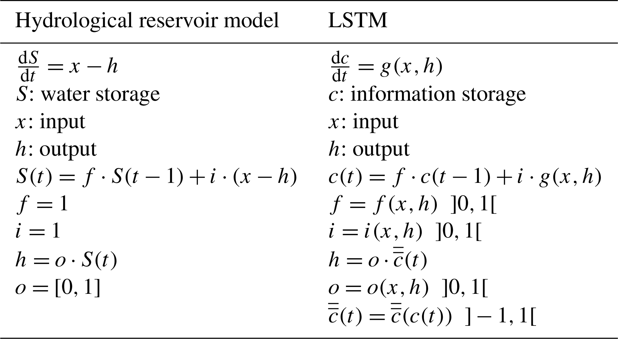
In many ways, the structure underlying a cell state of the LSTM architecture is isomorphic to that of the hydrological reservoir model after the application to the latter of finite difference approximation of the ordinary differential equation. Table 1 (adapted from De la Fuente, 2021) shows that the input, output, and forget gates in the LSTM represent scalar dynamical functions (asymptotic to 0 and 1). These correspond to the scalar constant-valued conductivity coefficients used in the linear reservoir model, in the sense that each controls the flow rate of time-variable quantities into and out of the corresponding cell state. Thus, while the LSTM functions g(t) and represent non-linear transformations, they can be understood to be identity functions in the case of the linear reservoir. In other words, the LSTM gate operators and transformations cause it to behave analogously to a non-linear reservoir.
Going further, the variable S in the linear reservoir formulation represents the aggregate physical state of the system, which can comprise multiple physically interpretable components such as snow accumulation, moisture in different parts of the soil system, storage in the channel network, etc. Similarly, variable c in the LSTM formulation represents the aggregate informational state of the system, which can comprise multiple components that are relevant to the predictive task at hand.
Importantly, this informational state of the LSTM can be regularized to obey conservation (mass, energy, or any other entity) by ensuring that its inputs are properly normalized and handled (Hoedt et al., 2021). However, in the more general sense, any source of informative data (such as precipitation, temperature, radiation, wind speed, humidity, static attributes, etc.) can be used to drive the evolution of the cell states. This multisource nature of the data ingestible by an LSTM model both improves its predictive power and complicates the interpretability of what the cell states are storing.
In summary, the analogy between the hydrological reservoir and LSTM is useful for elucidating the functioning of the representation. However, the direct transformation between one and the other (specifically about the parameters learned) is not possible due to the non-linear nature of the gates and the multiple sources of data used as inputs. Moreover, there are some differences between them that do not enable direct translation.
2.3 Differences with the hydrological reservoir model
Despite the aforementioned structural similarities, there are also some differences between an LSTM cell and the hydrological reservoir model, such as how the state variable is tracked and how context dependence informs the behaviors of the gates.
2.3.1 Tracking the evolution of the state
Some of the first applications of LSTMs were in the context of speech recognition (Graves et al., 2004) and natural language modeling (Gers and Schmidhuber, 2001). In these areas, two primary assumptions are typically applied that may not hold in the dynamic environmental system: (a) a finite relevant sequence length (finite memory time scale), and the consequent possibility of (b) a non-informative system state initialization. These assumptions can create challenges when applying LSTM to hydrological systems.
In linguistics, the idea is that symbols (letters and/or words) that have previously appeared many sentences or paragraphs earlier will typically provide less contextual information than more recent ones. This standard LSTM formulation, therefore, assumes that some finite number of sequentially ordered previous symbols will contain all (or most) of the relevant information required to establish the current context. We can think therefore that all the information needed is then summarized by the cell states (memory) of the model. Accordingly, all the symbols that are further away in the past than some specified sequence length can be ignored. This allows for the cell states to be initialized to zero (without information) at the beginning of the sequence.
This structure may make sense when dealing with linguistic applications; however, the assumption that the information in the cell state is dependent on a finite length of history does not, in general, align with how predictive context is established in a dynamical environmental system. For example, the information stored in mass-related hydrological state variables (e.g., the water content in the soil, groundwater levels, snowpack, etc.) can often be the consequence of a very long history of conditions and events that have occurred in the past. Thus, whereas in certain situations it might make sense for a relevant state variable to depend on only a finite-length history of past events (e.g., ephemeral snowpacks may be only informative about conditions since the onset of sufficiently cold weather for precipitation to occur in the form of snow), in many other situations the current wetness/energy state of the system may depend on an effectively indeterminate sequence length.
In such a hydrological system, where long-term memory effects can be important, the use of the standard LSTM assumption of a finite relevant sequence length could mean that valuable historical information present in the data is not optimally exploited. One way to account for that information would be to implement an informative (e.g., non-zero) initial condition when implementing the LSTM with a finite sequence length. Another way would be to extend the sequence length until errors in the initialization of the cell states are rendered minimal/unimportant. However, the more common approach is to have different strategies for the calibration and evaluation of an LSTM model. For calibration, the model uses the assumption of finite relevant sequence length and zero initialization of the cell state (sequence-to-one); whereas for the evaluation, the model is run sequentially for the entire evaluation period without reinitialization of the state variable (sequence-to-sequence). That approach solves in some way the issue of how much information is stored in the cell state; however, the internal parameters of the model remain calibrated so as to manage only the information contained within the sequence length.
Moreover, for dynamical environmental systems, the issues of cell-state initialization and selection of relevant sequence lengths are highly coupled. Without addressing this potential source of information loss, a model based on the traditional LSTM architecture arguably would be incapable of exploiting all the information regarding longer-term dependencies on conditions that predate the specified sequence length; for example, the long-term decadal and multidecadal dependencies that can affect the evolution of the North American precipitation system.
Having said this, the use of a fixed (finite) sequence length can be extremely useful for model development, as it facilitates the randomization of data presented to the model during the calibration process, which helps to ensure better calibration results and superior generalization performance. Proper randomization ensures that the data used for calibration and evaluation are statistically representative of the full range of environmental conditions for which the model is expected to provide reliable predictions (Chen et al., 2022; Guo et al., 2020; Zheng et al., 2018). By contrast, when developing models of the dynamical evolution of environmental systems with potentially long memory time scales, a more suitable formulation is one in which the effective memory length can be both variable and indeterminately long as needed (Zheng et al., 2022).
2.3.2 Gating behavior
Another difference between the LSTM and hydrological reservoir structures relates to the behaviors of the gates. Whereas the input gate of the hydrological reservoir is typically an identify function, and the output and forget gates (o(t) and f(t)) are typically assumed to depend mainly on the current state of the system, the three corresponding LSTM gates can vary dynamically in a manner that is controlled by the system inputs and outputs.
Consider the examples mentioned in Sect. 2.2, where we discussed the possibility of seasonal hydrological patterns/trends affecting the hydrological behavior of the gating mechanisms. In this context, it seems highly improbable that a gating representation based on knowledge of only the current system state, inputs, and outputs would be able to learn how to exploit relevant information about such seasonality. While it is possible to implement the standard LSTM architecture in such a manner that it can use sequences of past-lagged input and output data (up to some pre-determined sequence length) to also influence the operations of the gates, this can further complicate the problem of interpretability, by making it more difficult to disentangle the relationships between the sequence length, learned gating context, and the number of cell states needed.
To address the aforementioned issues (tracking of the state and contextual information in the gates), we propose an alternative LSTM-like architecture (hereafter referred to as HydroLSTM) that more closely aligns with hydrological understanding, while retaining the behavioral strengths of the traditional LSTM. The alternative structure continues to use the standard LSTM equations for the gates (i(t), o(t), and f(t)), cell states (c(t)), and outputs (h(t)), but makes two important changes. First, the cell states are continually updated from the beginning to the end of the available dataset while maintaining the sequential ordering of the input drivers. This ensures that the cell states represent Markovian memories that are effectively of indeterminate length (as in traditional hydrological modeling, initialization is done only once at the beginning of the simulation period). Second, the gates are allowed to learn behaviors that depend on a fixed, user-specifiable sequence of past-lagged data values that can represent (seasonal) memory of what has happened in the recent past. Accordingly, each cell state of the HydroLSTM uses the following equations:
where σ represents the sigmoid function, tanh is the hyperbolic tangent function, W and U are trainable weights, and b is a trainable bias term. All of the elements in the equations are vectors, where W, b, and x have the dimension of the number of dynamic inputs, and the functions i(t), f(t), o(t), c(t), and h(t) are scalars for a single cell state or vectors in the case that more than one cell in parallel is specified by the user. The symbol τ represents the lagged previous time steps, and j indicates the number of inputs (e.g., meteorological forcings). The “memory” term is a hyperparameter that specifies the sequence length used for determining gating behavior.
Figure 1 provides a conceptual illustration of the architectural differences between the LSTM and the HydroLSTM. The specific LSTM representation shown here (Fig. 1a) implements a sequence-to-one input–output mapping so as to better match the representation used in traditional hydrological modeling. The figure highlights how the LSTM representation must be evolved from an initialized cell state (typically zero) over some specified sequence length of past data () each time a prediction is required (e.g., for Q25, for Q26, and so on). This formulation limits the effective memory of the system to be shorter than or equal to the specified sequence length. The learned weights that determine gating behavior at each time step (arrows in the figure) remain constant across the sequence length (e.g., represented by the same size arrow for each time inside the sequence length). Note that the gating dynamics are only controlled by data from the current time step. Further, the same input data values must be processed several times when learning the correct values for successive current cell states.
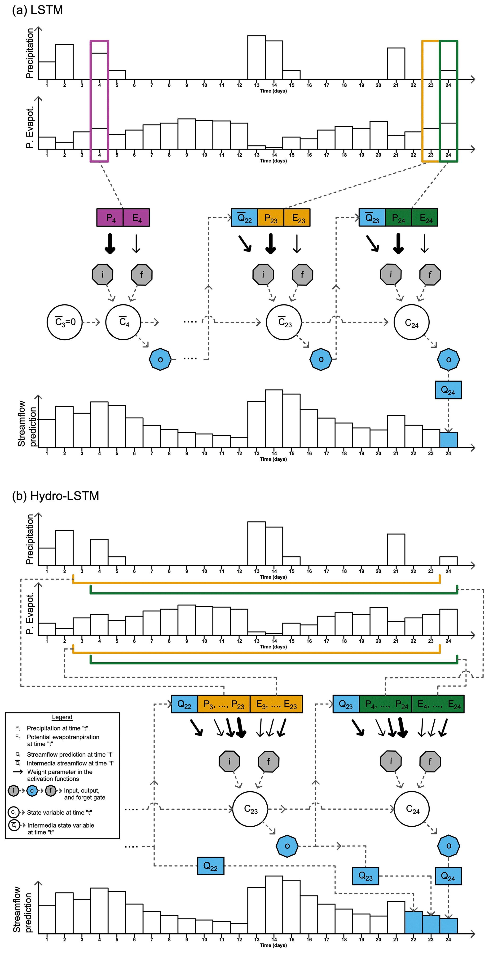
Figure 1Conceptual illustration of the LSTM and HydroLSTM representation. In this example, the LSTM (a) uses 20 d of past sequence data to determine the cell state value, while the HydroLSTM (b) uses 20 d of past sequence data to determine the gating behavior.
By contrast, while using the same input data, the HydroLSTM representation (Fig. 1b) initializes the cell states only once at the beginning of the time-ordered dataset (typically , but could be set to some other user-determined value). Accordingly, the state value C24 is updated based on C23, and so on. In this representation, the specified sequence length is used only within the gates to determine their gating behavior. We will show later (Sect. 5.1.3) that analysis of the corresponding learned weights (wider arrows) facilitates valuable hydrological interpretation.
Another interpretation of the difference between LSTM and HydroLSTM can be found in terms of the Markovian characteristic of the representation. LSTM represents the system as a fully Markovian process during the evaluation (but not during calibration), while HydroLSTM only considers the updating of the state in a Markovian manner. This happens because HydroLSTM uses more than the current data to define the behavior of the gates, which can be seen as a part of the past information being stored in the state variable, and another part being stored in the gates. For this reason, HydroLSTM can be understood as an intermediate level between a Markovian process (LSTM) and a non-Markovian process such as in transformers (Vaswani et al., 2017). However, which approach, fully Markovian or semi-Markovian, is more suitable or representative of a catchment with lumped data remains an open question.
We conduct two kinds of experiments to examine the behaviors of the standard LSTM and HydroLSTM representations:
-
In the first experiment, we examine three main aspects of the HydroLSTM and LSTM representations when they are calibrated for a single catchment: (a) architectural efficiency (parsimony) as measured by the number of cell states, (b) effectiveness as measured by predictive performance, and (c) interpretability of the learned weights of the HydroLSTM gates.
-
In the second experiment, we examine what can be learned about catchment memory time scale and its possible relationship to catchment attributes, by applying the HydroLSTM to a much larger number of catchments (always calibrating one model per catchment).
Details of the experiments are provided in Sects. 5 and 6. Here we present the overarching methods.
4.1 Data
Both sets of experiments use daily streamflow as the target output, and precipitation and temperature as meteorological data input, taken from the CAMELS dataset (Newman et al., 2014). Daily minimum and maximum temperature information available through the extension of the original meteorological forcing developed by Addor et al. (2017) is used to compute a reference crop evapotranspiration using the Hargreaves and Samani (1985) equation as an approximation to potential evapotranspiration. While the reference crop evapotranspiration must be adjusted for land use to obtain corrected estimates of potential evapotranspiration, we did not directly apply this correction and instead allowed the adjustment to be implicitly learned by the model for each catchment. Accordingly, precipitation and reference crop evapotranspiration (here simply called “evapotranspiration”) are used as the drivers of streamflow generation without the addition of information about catchment attributes (given that all the catchments are trained locally).
The temporally extended dataset is for the period 1 January 1980 to 31 December 2008, (approximately 28 water years). We split the data into calibration, selection, and evaluation periods as indicated below (these are commonly referred to as training, validation, and testing periods, respectively, in the ML literature).
-
Calibration (training, 20 water years): 1 January 1980 to 30 September 2000 (70.8 % of the dataset). The first 9 months (1 January to 30 September 1980) was used only for system initialization, and the rest was used for model (parameter) calibration.
-
Selection (validation, 4 water years): 1 October 2000 to 30 September 2004 (14.2 % of the dataset). This period was used to select the best-learned weights across all the epochs used in the calibration.
-
Evaluation (testing, 4.25 water years): 1 October 2004 to 31 December 2008 (15 % of the dataset). This period was used to assess generalization performance.
4.2 Machine-learning setup
To ensure a fair analysis of the architectures, we set up the implementation in such a manner that the only differences are the architectures themselves. The ranges over which the parameters vary, and the characteristics that define this setup, were adopted from traditional values commonly used in LSTM-based modeling research. Our purpose was to establish a common framework for evaluation, rather than to design some “best possible setup” which could be tweaked to favor one or other of the representations. As such, we implemented the following:
-
Only one hidden layer was used, with the number of cell states in that layer being the hyperparameter to be explored. All of these cell states were fully connected with the input and the output layers. The number of data lags for each input variable used to construct the input layer was also treated as a hyperparameter to be explored.
-
Uniform Glorot initialization of all weights and bias terms was used (Glorot and Bengio, 2010), as is suitable for networks when sigmoid functions are involved.
-
Both architectures were implemented using the same (sigmoid) activation functions. We did experiment with other activation functions, but do not report those results here. More research is required to determine whether specific activation functions are particularly suitable for hydrological applications.
-
The calibration was conducted for 512 epochs, from which the weights and biases were selected as those achieving the lowest selection period error at any point during calibration. Based on preliminary catchment-by-catchment testing, the batch size was fixed to be 8 d.
-
Parameter optimization was conducted using the stochastic Adam optimizer (Kingma and Ba, 2017) with a learning rate fixed at 0.0001.
-
The loss function used was the SmoothL1norm (Huber, 1964), which combines an L2 norm for a value lower than a specific threshold and an L1 norm for values higher than that. The reason is that this norm is less sensitive than mean square error (MSE) to outliers, which helps to prevent exploding gradients.
-
Because we seek a parsimonious representation, dropout was not implemented. Instead, stochasticity was achieved using an ensemble of 20 runs for each hyperparameter setting.
-
For each variable, a mean normalization procedure was implemented by subtracting the mean and dividing it by the range for each variable.
-
Evaluation period performance was assessed using the Kling–Gupta efficiency metric (KGE, Gupta et al., 2009).
Streamflow prediction models, based on the LSTM and HydroLSTM architectures, were developed and calibrated “locally” for each of these catchments (including parameters and hyperparameter combinations). In other words, only local catchment data were used for model development, and those models, therefore, represent the best possible predictive performance achievable at those locations using those architectures, without access to potentially useful information from any of the other catchments.
Note that important elements of the calibration procedure are data selection and stochasticity. For the LSTM, a random selection of subsamples in each batch used during calibration helps to achieve a rapid convergence (Kratzert et al., 2018; Song et al., 2020), and thus the standard procedure was used. By contrast, for the HydroLSTM, the data must be fed sequentially, and therefore the data in each batch are sorted in this way.
Further, the calibration of both representations is sensitive to the initialization of the parameters, and thus 20 different random parameter initializations were implemented for each hyperparameter combination. The mean performance achieved for those 20 different models was taken to be representative of the distribution of performance.
Given that the HydroLSTM structure requires sequential processing of the data, the corresponding state variable c(t) must be stored and used across all the time series even between batches and epochs. Consequently, the initialization of the cell states at the beginning of the calibration could be to some arbitrary value (zero or a randomly selected value). However, when iterating over multiple epochs (using the same calibration dataset), the cell states were initialized to their values obtained at the end of the time series, these being suitable initialization values for the next epoch in keeping with the fact that hydrological conditions at the beginning and end of water years tend to be similar.
In this experiment, we compare the architectural efficiency (parsimony as measured by the number of cell states) and effectiveness (as measured by predictive performance) of the HydroLSTM and LSTM over the 10 selected catchments. It is important to mention here that we train one model per catchment, given that our goal is to learn a parsimonious representation for each one. We acknowledge that this approach is not commonly used, and instead many studies calibrate a global model (calibration to many catchments at the same time). However, a global model is commonly used when the goal is to demonstrate the temporal or spatial consistency of the LSTM representation, and to demonstrate the benefit of transferring learning between catchments. This is different from our goal. Moreover, a global model can probably deliver better performance than a single LSTM model but with an internal representation (number of cells) that is not parsimonious for a specific catchment, and therefore not useful for our analysis.
For purposes of discussion, we show the results for only two catchments from different hydrological regimes; the figures for all 10 catchments are included in Appendix A.
5.1 Methodological details
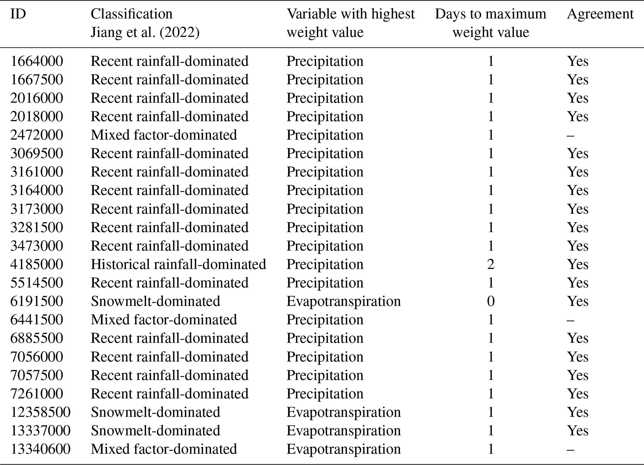
Ten catchments with different hydrometeorological behavior were randomly selected from the CAMELS dataset to perform a comparison of the LSTM and HydroLSTM architectures. Two catchments were selected to represent each of the homogeneous regions identified by Jiang et al. (2022) based on behaviors learned by an LSTM-based modeling approach applied to flow peak prediction (see Table 2 and Fig. 2). The three main flooding mechanisms presented in that research can be roughly described as events where the main driver is (1) the precipitation of the same or previous day (recent rainfall-dominated), (2) precipitation from several past days or possibly weeks (historical rainfall-dominated), and (3) snowmelt-dominated where temperature controls the streamflow. For more details about this classification, readers are referred to Jiang et al. (2022).
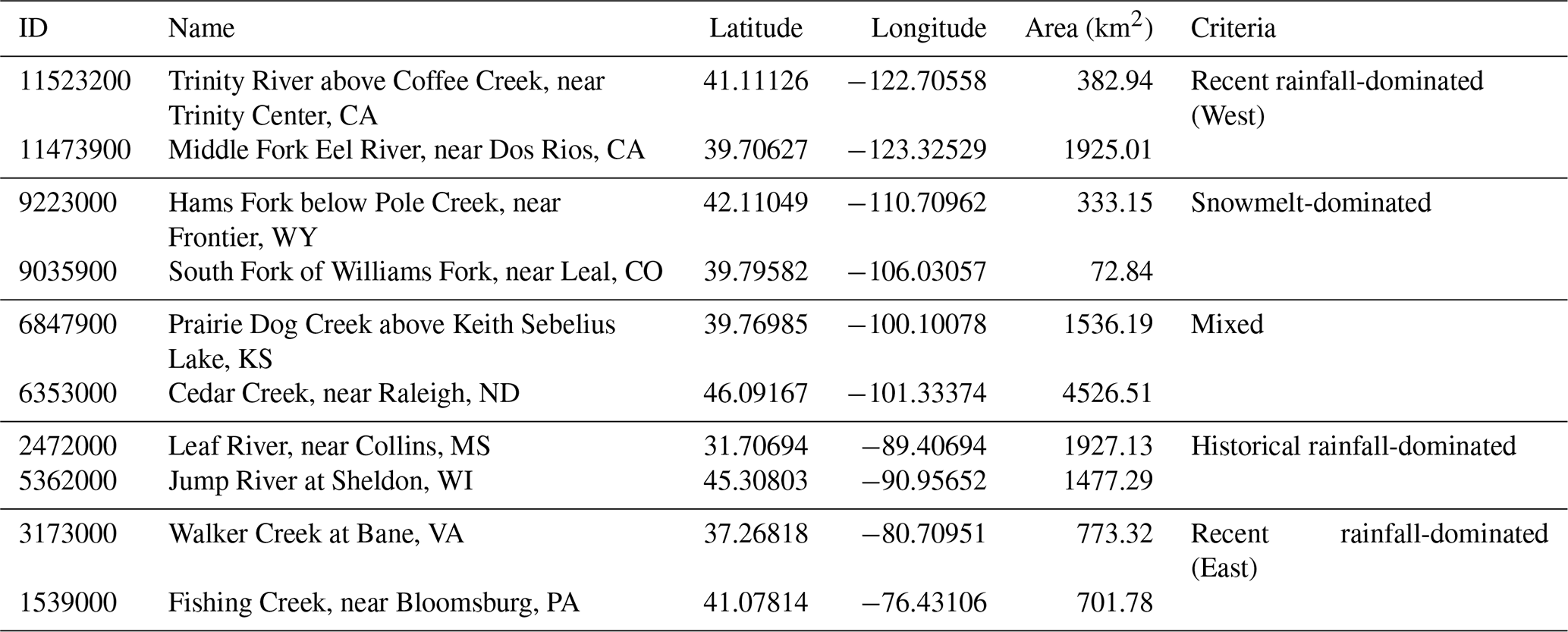
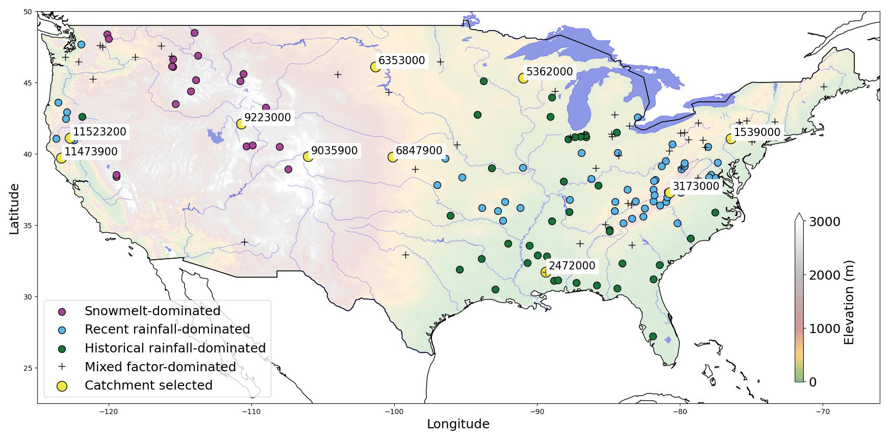
Figure 2Catchments selected in this study, adapted from Jiang et al. (2022). Yellow circles represent the catchments analyzed and the other colors represent the three flooding mechanisms presented by Jiang et al. (2022).
With the ML setup constraints defined previously, the only hyperparameters that must be tuned via grid search are the number of cell states and the lagged memory length (for LSTM this is the sequence length, and for HydroLSTM this is the number of lagged time steps used to determine the gating behavior). For this experiment, the numbers of cell states were varied to be 1, 2, 3, 4, 8, and 16. For the lagged-memory hyperparameter, we varied the value as powers of 2 (i.e., using 2, 4, 8, 16, 32, 64, 128, and 256 lagged days) to account for the fact that each extra day tends to provide decreasing amounts of information as the number of lags is increased.
In keeping with the principle of parsimony, we identified the “simplest” LSTM and HydroLSTM representations as being the ones with the smallest number of cell states for “comparable” predictive performance. To determine this level of similar performance, we conducted a statistical comparison (at the p=0.1 significance level) between the mean performance of the 20 realizations per hyperparameter (number of cells, and lagged days) and a selected hyperparameter configuration as the reference. This reference was defined as the best performance achieved by Hydro-LSTM when using one or two cells (red * in Fig. 3). Hyperparameter configurations with non-significant difference in the mean for both representations are shown with a black asterisk.
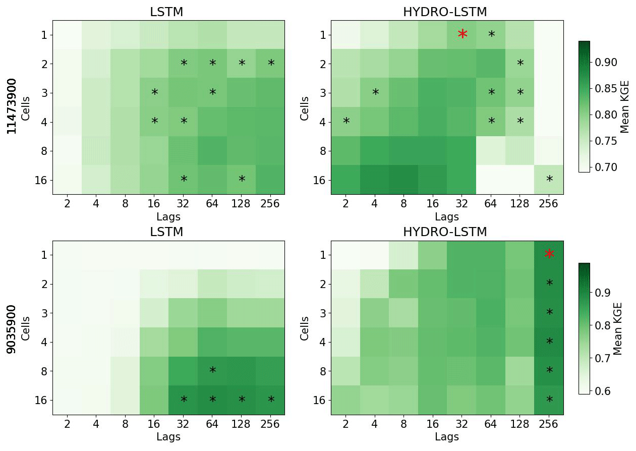
Figure 3Performance heatmap for different hyperparameter sets, number of cell states, and lag days. Rows: Catchment studied. Columns: representation. An asterisk shows the hyperparameter sets with no statistical difference in the mean with respect to the red asterisk for each catchment. The green color (good performance) is presented closer to the row of #1cell for HydroLSTM than LSTM representation, which is an indication of parsimony of the former.
5.2 Number of cell states
Figure 3 shows the results for two catchments, where we plot heatmaps of mean KGE performance for each combination of the number of cell states (from 1 to 16) and the number of lagged days (from 2 to 256) tested. Darker green indicates higher KGE performance (optimal KGE=1). Each row of subplots corresponds to a catchment while the left column is for LSTM and the right column is for HydroLSTM. The cell–lag combinations for which the mean performance differences are not statistically significant are marked using the asterisk symbol. From these, the red asterisk shows the hyperparameter combination used for doing the statistical analyses. We see that for many hyperparameter combinations, the performance is statistically similar.
For both catchments presented in Fig. 3, a HydroLSTM-based model having only a single cell state performs (on average) as well as an LSTM-based model having a larger number of cell states. For the Eel River, CA, (ID 11473900) both architectures obtain good levels of KGE performance (above 0.8) using 3 to 4 cell states, even though slightly better results can be achieved using 16 cell states. This makes sense, given that the catchment is in a region where recent rainfall dominates the generation of streamflow and where several state/storage components (such as surface, subsurface, groundwater, channel network, etc.) can be expected to be relevant to the streamflow generation process. Nonetheless, the HydroLSTM-based model with only a single cell state provides comparable performance to an LSTM-based model having two cell states, when both are provided with the same lagged input sequence length.
Meanwhile, the South Fork of Williams Fork, CO, (ID 9035900) is in the Front Range of the Rocky Mountains, where snow accumulation and melt dynamics strongly govern streamflow generation. Here, the difference between the HydroLSTM and LSTM is quite marked. The HydroLSTM with a single cell state (with 256 d lagged inputs) obtains extremely high performance (mean KGE>0.85) while adding more cell states does not result in further statistical improvement. By contrast, the LSTM-based model requires at least eight cell states (with >32 d lagged inputs) to obtain comparable performance, which is a much less parsimonious characterization and makes interpretability much more difficult.
Figure 4a expands upon Fig. 3 by summarizing the results for all 10 of the catchments studied. In all cases but one, the LSTM requires more than one cell state to achieve the same performance as HydroLSTM. This is another indication that LSTM is not creating a parsimonious characterization of the input–state–output relationship. For instance, the catchments Trinity River (ID 11523200), Leaf River (ID 2472000), and Fishing Creek (ID 1539000) show the largest differences in the number of cell states between both representations, 1 cell in HydroLSTM versus 16 cells in LSTM.
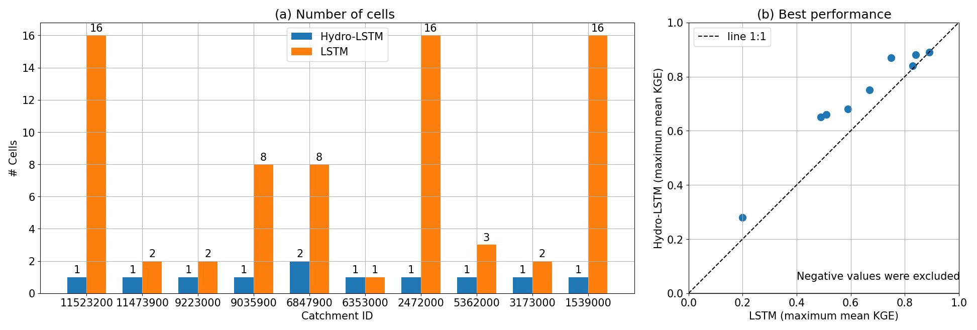
Figure 4Summary of cell-state parsimony and KGE performance. (a) Comparison of the minimum number of cells needed for each representation having a non-statistical difference in the mean performance. (b) Best performance of each representation across all the hyperparameter sets explored.
5.3 Comparison in terms of the best performance
We next compare the best performance between HydroLSTM-based and LSTM-based models across the entire range of numbers of cell states and input lags. Figure 4b shows the best mean KGE performance for each of the 10 catchments. The values fall close to the 1:1 line indicating similar overall performance using the HydroLSTM and LSTM architectures, which is desirable given their similarities in the structure. Table B1 in the Appendix presents the values from Fig. 4b with the addition of the performance obtained using an external library for LSTM (NeuralHydrology, Kratzert et al., 2022) over the 10 catchments studied. These results show that the KGE values are in the range for both implementations of LSTM, meaning that our implementation of LSTM performs consistently with the external source.
Of course, this observation of “similar” performance is not intended as a general conclusion, given that numerous versions of the LSTM architecture exist, and more emerge every year (e.g., LSTMs with peephole connections, GRUs, bidirectional LSTMs, LSTMs with attention, etc.). It must be kept in mind that we have tested only the simplest possible LSTM structure, to be able to interpret it using hydrological reservoir concepts. Further, the goal of this study is not to find a representation that outperforms the LSTM performance (or the current state of the art in recurrent neural networks), but instead to explore whether similar performance can be obtained with a more parsimonious and physically interpretable architecture.
5.4 Temporal pattern in the distribution of weight
For all but one of the 10 catchments represented by Fig. 4a, we found that good performance can be obtained by a HydroLSTM-based model having only a single cell state. This is convenient, as it allows us to compare (across catchments) the patterns of the “gate weights” learned for each model in the 20-member ensemble. For this purpose, we examine the results obtained for two selected catchments, one being rainfall-dominated and the other being snowmelt-dominated. Specifically, Fig. 5 shows the distributions of the gate weights, associated with the lagged precipitation and potential evapotranspiration inputs. Each catchment is evaluated using a single-cell HydroLSTM-based model with lag memory as a hyperparameter (the figure shows the weights from the best-performing model). This figure illustrates the systematic trends present in the time-lagged patterns of the distributions of the weights. In general, the weights show the highest values at earlier lag times (e.g., <2 d), indicating that fast behaviors control the response of the gates. This is aligned with the LSTM approach where only one single weight associated with the closest time is used. However, it is clear that additional previous days also play a role in some cases. At longer lag times (e.g., >10 d) the weight distributions tend to encompass zero, indicating that the relative importance of past information decreases rapidly, and it follows a more random behavior. That suggests that L-norm regularization could be used to better constrain these values during calibration (and that such values could be interpreted as effectively zero). For this study, we decided not to train with L-norm regularization. Rather than seeking a minimal number of weights, we are interested in the general interpretability that might be associated with the time-lagged patterns seen in the trained weights, and whether these patterns might represent specific characteristics associated with different catchment “types”.
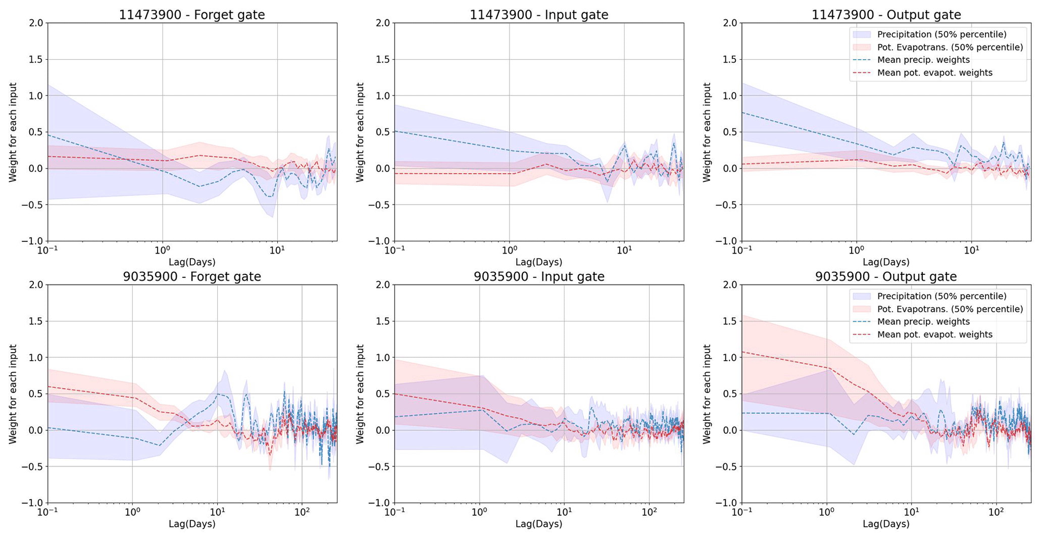
Figure 5Weight distribution in the three gates for two of the catchments studied. The upper row is a catchment in a recent rainfall-dominated region. The lower row is a catchment in a snowmelt-dominated region. The confidence interval is the result of running 20 models with random initialization.
The interquartile range of 20 models (Fig. 5) indicates high dispersion at early lag times, indicating a high degree of freedom and equifinality issues in the value that a specific weight can take. In some way, this is associated with the multiple possible combinations in the operation of the gates working together, and the lack of regularization over that. However, despite the dispersion, consistent patterns emerge from all the catchments studied, especially for the output gate (which is responsible for the streamflow generation). This is a novel finding because weight values in ML models are typically considered to be random and non-interpretable.
In this regard, we note that the output hydrological response of the Eel River, CA, (ID11473900, upper row) is governed by recent rainfall events (Table 2), which aligns well with the high weighting assigned to precipitation at time zero ( in the figure) in all of the gates, and particularly in the output gate that directly controls the streamflow response. The rapid decline (toward zero) in weight magnitude with time lag is consistent with a system having a relatively short hydrological memory. Further, the weights associated with potential evapotranspiration tend to be very close to zero, indicating its relative lack of importance in governing streamflow generation. These characteristics are consistent with the hydrological classification reported by Jiang et al. (2022).
By contrast, the results shown for the snowmelt-dominated catchment (lower row of Fig. 5) are quite different. Now we see significantly larger weight values associated with potential evapotranspiration (around 1.0 for the first days) which is strongly determined by air temperature, which in turn is the primary driver for snowmelt dynamics. Moreover, the weights remain at high values for as long as 10–20 d (compared with the values close to zero after that period), which is consistent with the time durations associated with energy/heat accumulation required for the melting process to begin resulting in a significant generation of streamflow.
Results for the other eight catchments are presented in Appendix C. In general, the weight patterns correspond well with the hydrological classification presented in Table 2. Models for the “western recent rainfall-dominated” catchments assign higher weights to recent precipitation, while models for “snowmelt-dominated” catchments assign high weights to about 10+ d of potential evapotranspiration (as a surrogate for temperature). Models for the “historical rainfall-dominated” catchments assign high weights to several past days of precipitation (1–10 d), while models for “eastern recent rainfall-dominated” catchments have weight patterns indicating longer resident times in that part of the country (eastern). In general, these results support the idea that the learned weight patterns can encode useful information regarding the hydrometeorological characteristics of different catchments.
The patterns described can be understood as the primary response to streamflow given the higher weight values they present. However, other persistent patterns for longer lag times can be found for some catchments, such as the case of “snowmelt-dominated” catchments. We do not describe those patterns in detail given that we focus on demonstrating the relationship between weight distribution and hydrological signatures which are controlled by the primary response. We incorporate in the Supplement (Figs. S1 and S2) the same Figs. C1 and C2 with a uniform time scale (x axis) to help with the visualization of those secondary patterns.
5.5 Temporal patterns in the evolution of the cell state
Seeking further hydrological insights, we also examined the patterns in the temporal evolution of the (single) cell state obtained for the trained HydroLSTM models. Specifically, we examined the results obtained for the South Fork of Williams Fork, CO, catchment (ID9035900) for which the best KGE performance (over the 10 catchments) was obtained. However, despite having only one cell state and high performance, the cell state trajectories of the ensemble of 20 models displayed no mutually consistent trends, and therefore poor interpretability (Appendix B). Accordingly, we did not pursue such an analysis for the other catchments. We revisit this issue in the discussion section of the paper.
We are interested in the behavior of the HydroLSTM architecture when applied to a large diversity of catchments. Here, we specifically explore how the amount of lagged memory varies geographically. Since in the first experiment remarkably good KGE performance was obtained by use of a HydroLSTM architecture with only a single cell state (see Fig. 4a), we proceed by fixing the number of cell states at 1. This way the 588 catchments were calibrated with one cell and multiple lagged data to explore how the optimal number of sequence time lags used for gating varies across the country. Note that although an optimum number of cell states for each catchment could be estimated, this is a computationally expensive task that we will explore in future works.
6.1 Methodological details
In this experiment, we expanded the number of catchments used from the CAMELS dataset in the first experiment (10 catchments). From the 671 catchments originally available in the dataset, we used the 588 catchments that have streamflow data for the entire calibration, selection, and evaluation period presented in Sect. 4.1, and one HydroLSTM-based model was calibrated for each of the catchments selected. These 588 catchments represent similar hydroclimatological diversity as the original 671.
At this point we are not interested in determining the best-performing from HydroLSTM-based model, instead, we are looking for interpretability under a parsimonious representation (one cell). From the perspective of this goal, while adding more cells could help make marginal improvements to performance, the consequence would be a considerable reduction in what can be learned. The same situation would happen if we calibrated a global HydroLSTM model on the 588 catchments: it would be very hard to analyze specific behaviors when examining a global model consisting of hundreds of cells (a very common representation for global ML-based models). Therefore, all the analysis reported here is based on calibrating only a one cell-state model per catchment. Under this constraint, different settings of the “lag memory” hyperparameter (i.e., 4, 8, 16, 32, 64, 128, and 256 lagged days) are studied.
6.2 Results
The cumulative distribution (CDF) of KGE performance is presented in Fig. 6a. As we provide the models with increased numbers of lagged inputs (consistent with increasing system memory time scales), the CDFs shift to the right (indicating improved overall performance). This seems reasonable, given that the models can access greater amounts of information regarding the history of the corresponding catchment system. However, for catchments with KGE>0.4, performance improvements saturate between 64 and 256 d. For KGE<0.4, the curve for 256 d is the best option, for which reason it was selected as the overall best lag. This is consistent with the 270 d sequence length reported by Kratzert et al. (2019) as being suitable when training a single LSTM model to represent the entire CAMELS dataset.
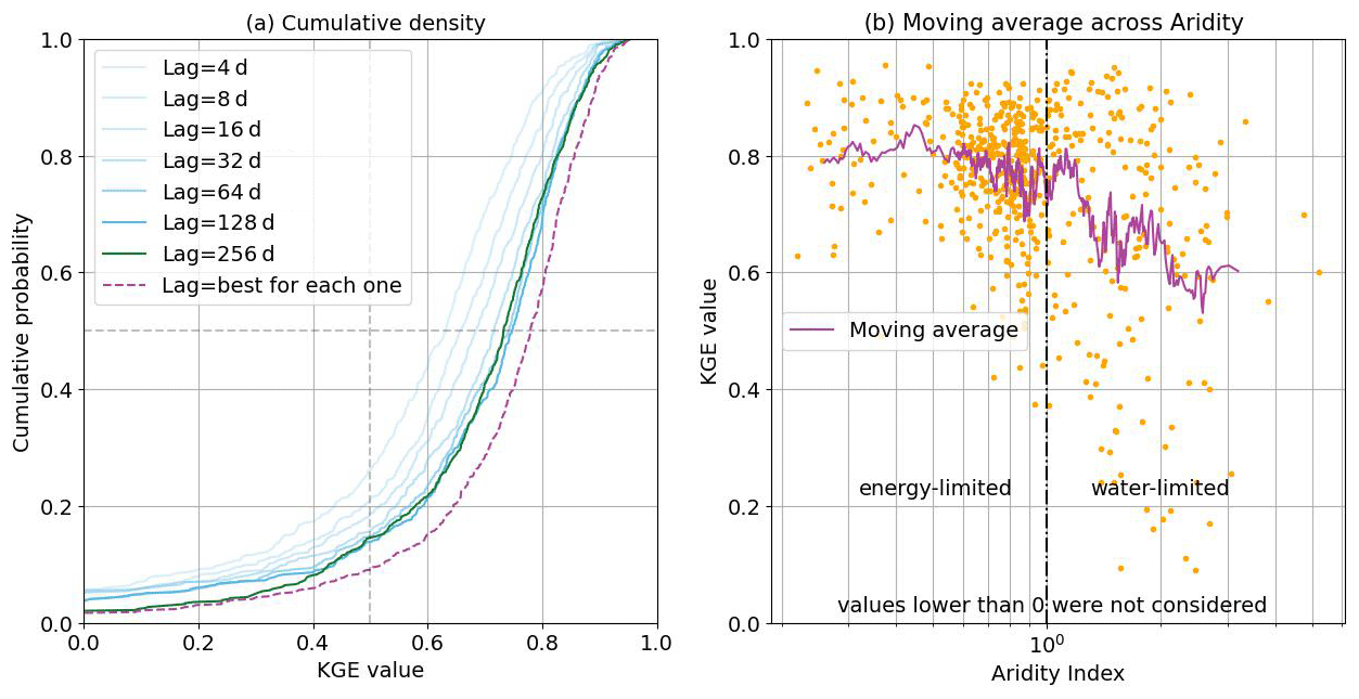
Figure 6HydroLSTM performance over 588 catchments (one model per catchment). (a) Cumulative density function for catchments trained using different amounts of lag memory (green and blue lines) and performance for the best catchment-specific lag (dashed purple line). (b) Performance versus aridity index (the purple line is a 15-catchment moving average) showing different behaviors for energy-limited and water-limited regions.
However, when we independently search for the optimal sequence length associated with each catchment, we obtain the red line, which is shifted even further to the right. This suggests that the use of a fixed sequence length (memory time scale) across the CONUS is not optimal and that better results can be obtained by allowing the sequence length to be determined along with the trainable parameters of the model. Arguably this makes sense since the system memory time scale can be expected to be a characteristic property of each catchment. Accordingly, when seeking to create a single “global” model that can be applied universally to all the catchments used for model development, it would be desirable for the chosen representational architecture to be sufficiently flexible to be able to learn this characteristic.
Figure D1 (Appendix D) presents the CDF and the scatter plot for 100 catchments calibrated locally with the LSTM external library versus HydroLSTM using the best lag for each catchment. This result complements our conclusions about the similar performance achievable by both representations (slightly better for HydroLSTM). However, as mentioned in Sect. 5.3, our goal is to find a more interpretable representation rather than finding a representation that outperforms LSTM.
As a step toward a global representation, Fig. 7 shows the spatial distribution of the optimal sequence length determined above (corresponding to the red line in Fig. 6a). Although some rough regional patterns are apparent, they do not stand out clearly. For example, longer sequence lengths seem to correspond to mountain ranges (Appalachian, Cascades, and Rocky Mountains), while shorter memory seems to be associated with smaller catchments that are far from major rivers. Thus, while one might expect (from a functional perspective) that sequence lengths should correspond to some distinguishable attributes of the catchments, geographic location is apparently not sufficient for this purpose. Our results suggest that a more detailed future investigation of how the optimal sequence length (as an indicator of system memory) corresponds to observable catchment attributes could prove to be useful and informative.
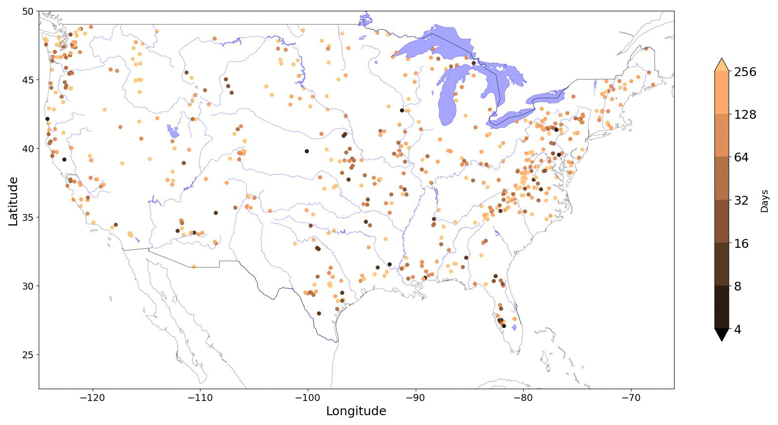
Figure 7Spatial distribution of the optimal sequence length determined for each catchment. No obvious pattern related to catchment attributes is apparent.
While it would be desirable to conduct a full comparison with the classification results reported by Jiang et al. (2022), this research was done using a different dataset, and only a few catchments are shared with the CAMELS dataset. In Table D1, we list the catchments in common and the main characteristics of the weight pattern (controlling variable and days for the maximum weight value) that we found. These results complement our findings (Sect. 5) that the weight patterns encode information regarding the hydrological behaviors of the catchments.
Following the analysis by De la Fuente et al. (2023), we also use the aridity index (AI) as another catchment attribute (beyond space location) to segregate the catchments and plot the optimal model KGE versus AI for all 588 catchments (Fig. 6b). We see that the moving average trend (over 15 catchments) and dispersion of KGE performance remain fairly stable in the energy-limited regime (AI between 0.25 and 0.6 mm mm−1), from which we can infer that the input–state–output relationships in such regions are reasonably well characterized using only precipitation and potential evapotranspiration (or temperature) as the system drivers. However, for water-limited regions, as the AI increases, the dispersion gets larger and the average model performance declines, suggesting that these two drivers alone (possibly along with data quality issues) are insufficiently informative to achieve good predictive performance. It is, of course, possible that the situation could be remedied by appropriate choice of a “better” representational architecture, as has been stated for many years in the hydrology literature (Pilgrim et al., 1988). However, the fact that De la Fuente et al. (2023) obtained similar results using three different representational approaches (two ML models and one spatially lumped process-based model) tends to suggest that the problem may lie with the data instead. Note also that the upper boundary of performance (∼0.9) remains relatively insensitive to the AI, even in the water-limited regions. The fact that performance is still high in some of the cases with high AI suggests that some other catchment attribute (such as slope, area, elevation, etc.) may also be relevant to the ability to achieve good model performance. However, it is clear that more work is required to disentangle the factors associated with overall model performance in arid regions.
Complementary to the findings of memory being catchment-specific (Fig. 6a) and the relationship between aridity and performance (Fig. 6b), we also examined model performance when the amount of lag memory is associated with different clusters of catchments. We hypothesize that for arid catchments, better predictive performance will typically require data with longer lags than for wet catchments. Accordingly, we defined four subgroups corresponding to different levels of aridity, while maintaining a minimum level of performance of KGE>0. Further, given that long memory time scales are typically expressed via baseflow, we restrict the analysis to catchments with a baseflow index (ratio of mean daily baseflow to mean daily discharge) above 0.5.
The results are shown in Fig. 8. We see that for catchments with AI<0.6, an optimal number of lagged days (defined by the highest median, red line) of input is around 64 (∼2 months), but performance is relatively insensitive to the number of lags. For catchments with and , we see more pronounced increasing trends in performance with the number of lags, with the optima being at 128 (∼4 months) and 256 (∼8 months) days, respectively. Finally, the water-limited catchments (AI>1) exhibit much greater sensitivity to memory time scales. In this preliminary study, the largest number of time lags examined was 256 d, but the results suggest that longer time scales would be worth investigating in future work. Overall, the results suggest a strong relationship between required memory time scales and aridity, which is consistent with the conclusions of De la Fuente et al. (2023), i.e., that improved representation of groundwater-related processes is required when modeling water-limited catchments. Moreover, it is crucial to recognize that catchment memory (in terms of lag memory) is influenced by various factors beyond just aridity (e.g. groundwater and surface water possess a very different degree of memory, therefore its influence on the overall memory in a catchment could change drastically). Therefore, it is not possible to strictly define the “best” lag for a specific level of aridity. Rather, we can only observe that a relationship exists, meaning that more research should be done to clarify this relationship.
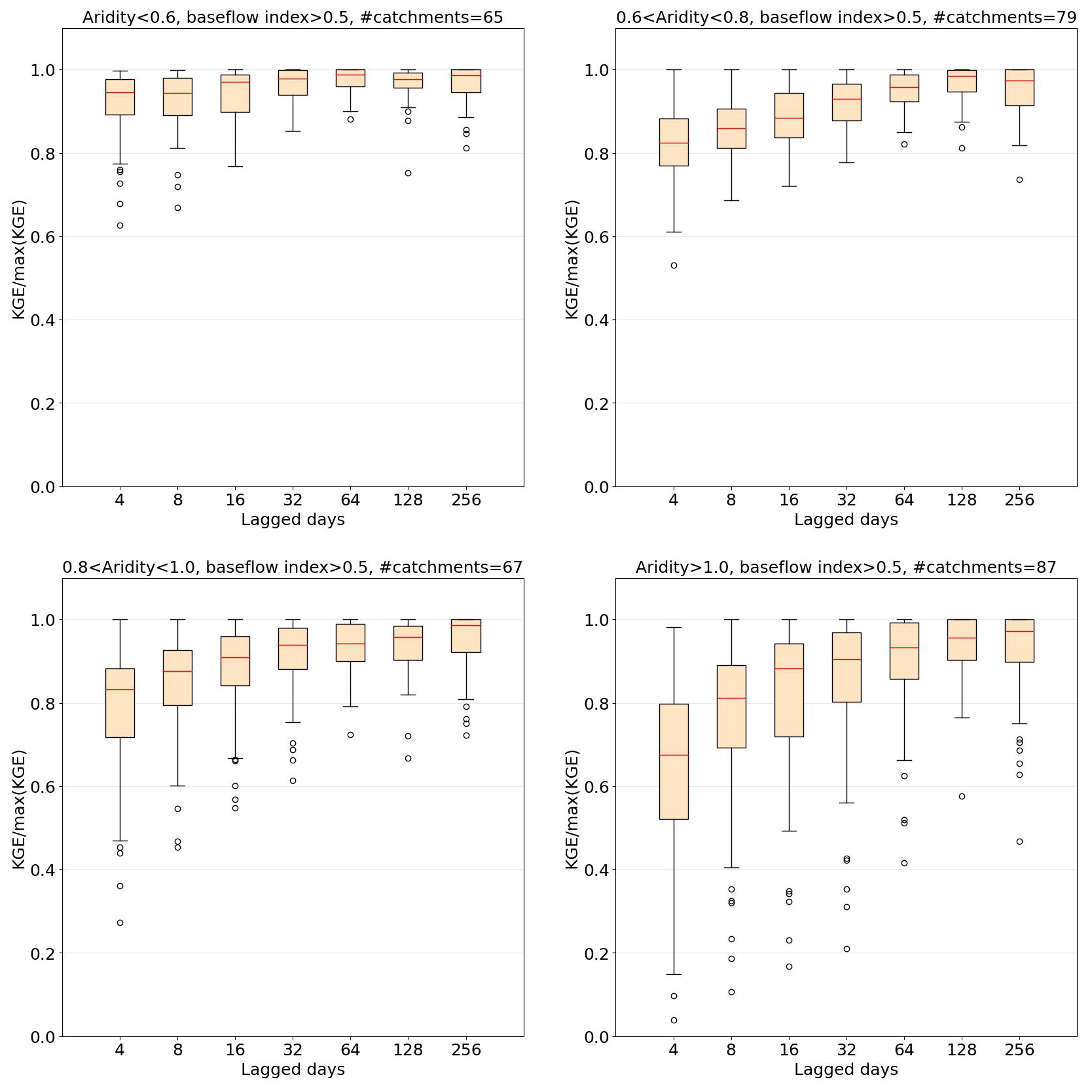
Figure 8HydroLSTM performance as a function of sequence length for four catchment subgroups associated with different levels of aridity. Wet (energy-limited) catchments are relatively insensitive to sequence length, while arid (water-limited) catchments require longer sequence length.
The main motivation for creating the HydroLSTM architecture was to explore how ML methodologies can better support the development of hydrological understanding, while thinking of the catchments as independent entities. However, this is not to imply that we do not believe in a broader approach to catchment hydrology. Instead, we seek to create the basis for achieving understanding from what a global LSTM type representation can learn about hydrology. For this reason, we have focused on the interpretable nature of the weights and cell states of catchment-specific HydroLSTM-based models.
7.1 Interpretation of the weighting pattern
Due to the high dimensionality and algorithmic complexity of typical ML-based representations, the learned weights are commonly considered to be non-interpretable (Fan et al., 2020). However, the weights that determine the behavior of each gate in the proposed HydroLSTM architecture can, when viewed as sets, be interpreted as representing features or convolutional filters that are applied at each time step to the sequence of lagged inputs. As such, these filters act to extract (via temporal convolution) contextual information about the recent hydrometeorological history that can be expected to govern the current response of the catchment.
An interpretation is that these filters serve as a compressed, low-dimensional, embedding of the information encoded in the high-dimensional space of the lagged inputs and weights. In other words, the information contained in hundreds of highly correlated lagged inputs is transformed into a small number of scalar values that succinctly express the information needed to determine the behaviors of the gates. This “information bottleneck” process (Parviainen, 2010) has been shown to perform well at dimensionality reduction and to help achieve linear scaling in calibration time. Accordingly, the relatively high dimensionality of inputs to a gate is not a serious problem, given that the compressed (latent) space tracks only the information required for determining catchment behaviors. In brief, the temporal patterns associated with the learned gating weights can be informative about what is being learned by the network.
Another hydrological interpretation of these patterns is associated with the classic use of unit hydrographs (Sherman, 1932; Lienhard, 1964; Rodríguez-Iturbe and Valdés, 1979) to represent streamflow. At each time step, we can think of the streamflow as the sum of baseflow and a runoff component. The baseflow component is highly correlated with the water storage in the catchment and thus it can be very well tracked by the state variable(s) of a model. On the other hand, the runoff component depends on the temporal pattern of distribution of the precipitation from the previous days. This means that a convolution filter (a unit hydrograph applied many times) over the past precipitation could represent that phenomenon well. Accordingly, the total streamflow can be considered to result from a mix between the two ways of processing the information (state versus context). Of course, at this moment we cannot be sure that HydroLSTM is performing such a separation, but certainly this way to process the data is not something new in hydrology.
While we have focused mainly on the interpretability of the output gate, the forget and input gates also provide interpretable information. However, because their interpretation is more closely tied to the state variable and the nature of the input employed, interpreting those gates directly is not as readily achieved without appropriate regularization of the states and inputs. For instance, the state variable may be storing diverse forms of pertinent information, making it difficult to determine the exact extent to which the model should remember or forget part of it. Currently, there are many research groups working on this kind of additional regularization, which imposes constraints on the storage of specific entities such as volume and energy. Therefore, we expect that more interpretability could be ascribed to the other gates in the near future.
7.2 Interpretation of the cell-state trajectories
As mentioned in the Introduction, architectural parsimony (expressed as a smaller number of state variables) can lead to better interpretability of the information encoded into a model. Here, we have demonstrated that the HydroLSTM approach enables a representation of catchment input–output dynamics to be achieved using only a relatively small number of cell states per catchment. However, even when we use only a single cell state to represent the storage dynamics of a catchment, this does not ensure a unique solution.
The reasons for this non-uniqueness are worth considering. It is important to note that the high model performance (as in Sect. 5.5) only ensures that the prediction, represented by h(t) Eq. (6), closely tracks the target (streamflow). However, given that h(t) is determined as the product of the output gate o(t) and a function of the cell state c(t) (i.e., ), it is clear that many different combinations of these trajectories can result in the same trajectory for h(t). Thus, given that the current implementation of HydroLSTM only weakly constrains the state variable-to-flux relationship (output gate), we should not expect to arrive at a unique representation for the cell state. To further constrain a HydroLSTM-based model to learn cell states (such as snow water equivalent, water table depth, soil moisture, etc.) that align with hydrological understanding, we will necessarily have to add extra information that regularizes the internal (latent space) behavior of the model. In ongoing work, we are exploring how the use of predefined weight patterns (such as those that follow Gamma or Poisson distributional shapes), and/or calibration to multiple catchments simultaneously while adding information regarding static catchment attributes, might help to better constrain the learned cell-state trajectories.
Further, it is worth noting that while the HydroLSTM and LSTM representations have access to the same information sources, they use that information in somewhat different ways. In the LSTM, the gates only have access to current time step information, and a significantly larger number of cell states is needed to obtain a given level of predictive performance. In other words, most of the information about past system history that is relevant to making accurate predictions is encoded into the cell states. By contrast, the HydroLSTM is provided with access to much of that same historical information via the sequences of lagged input data that are fed into the gating mechanisms, and therefore information regarding the current “state” of the system can be encoded via a smaller number of cell states. Given that both architectures provide comparable predictive performance through a different process of encoding the relevant information about the input–state–output dynamics of the catchment system, both representations can be considered to be valid.
We have proposed and tested a more interpretable LSTM architecture that better encodes the hydrological knowledge of how a catchment behaves. This gain in interpretability is achieved by modifying how the “state” of the system is tracked (sequentially from the beginning to the end of a historical dataset) and by providing the input, output, and forget gates with access to lagged sequences of historical data. We have named this modified architecture “HydroLSTM”, to acknowledge the inspiration obtained from the isomorphic similarities of its cell states to that of a hydrological reservoir model.
The HydroLSTM architecture provides comparable performance to the original LSTM while requiring fewer cell states (as was demonstrated using data from 10 catchments drawn from five hydroclimatically different regions). At the same time, the weights associated with the sequences of lagged inputs of each gate display patterns (i.e., express characteristic features) that can help in distinguishing between catchments from different regions. A detailed examination of the impact of sequence length (a hyperparameter related to system memory time scales) indicates that this is an important architectural aspect that varies with location and can (at least partially) be associated with aridity. An additional degree of flexibility that should be incorporated into future modeling frameworks would be the ability to learn the specific sequence length and weight patterns directly from the data. In this way, a globally applicable HydroLSTM architecture could be achieved and compared with a global LSTM model. However, our conclusions are only applicable to catchment-specific models. A similar argument can be made for learning how many cell states are needed while adhering to the principle of parsimony, but this would add an additional level of complexity in the architecture that must tackled after the issue of memory and weight patterns is solved.
We propose that the sequenced patterns of the weights encode hydrological signature properties. This should be further investigated on a broader set of catchments than was used for this analysis. If the behavior we demonstrated here is found to be robust on larger sample sizes, this would open up a pathway to exploring how clustering based on such signatures can help to characterize catchments in terms of their similarities and differences, a task that has proven challenging (Singh et al., 2014; Ali et al., 2012). We suspect that these weight patterns can eventually be regularized using fixed functional forms (e.g., by combining appropriate parametric basis functions) to reduce the number of parameters to be learned, and potentially further enhance hydrological interpretability by relating those parameters to catchment characteristics that are computable directly from data.
In conclusion, we have demonstrated that by “looking under the hood” of an ML representation it is possible to create ways to better extract useful information from the learning process while retaining all (or at least most) of its strengths. That is an indication of how powerful our representations are, and at the same time how limited our interpretations can be if we do not understand those representations deeply. For that reason, it behoves us to choose those representations carefully and to be prepared to adapt and improve them in response to what we learn from our scientific explorations.
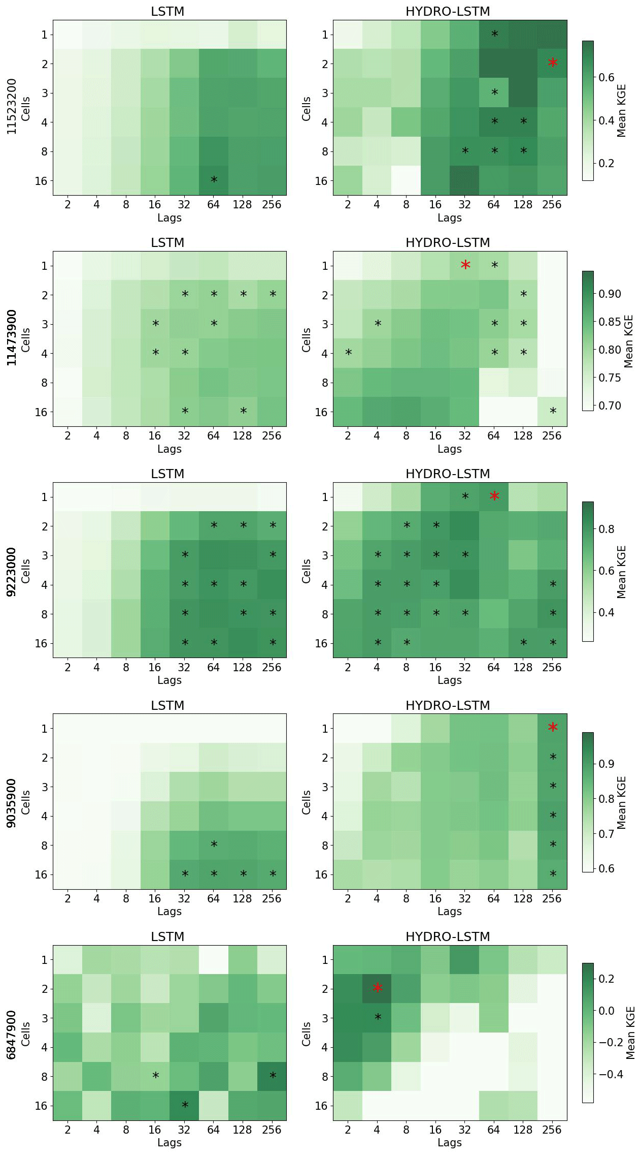
Figure A1Performance heatmap for different hyperparameter sets, number of cells, and lag days. Rows: Catchment studied. Columns: representation. An asterisk shows the hyperparameter sets with no statistical difference in the mean with respect to the red asterisk.
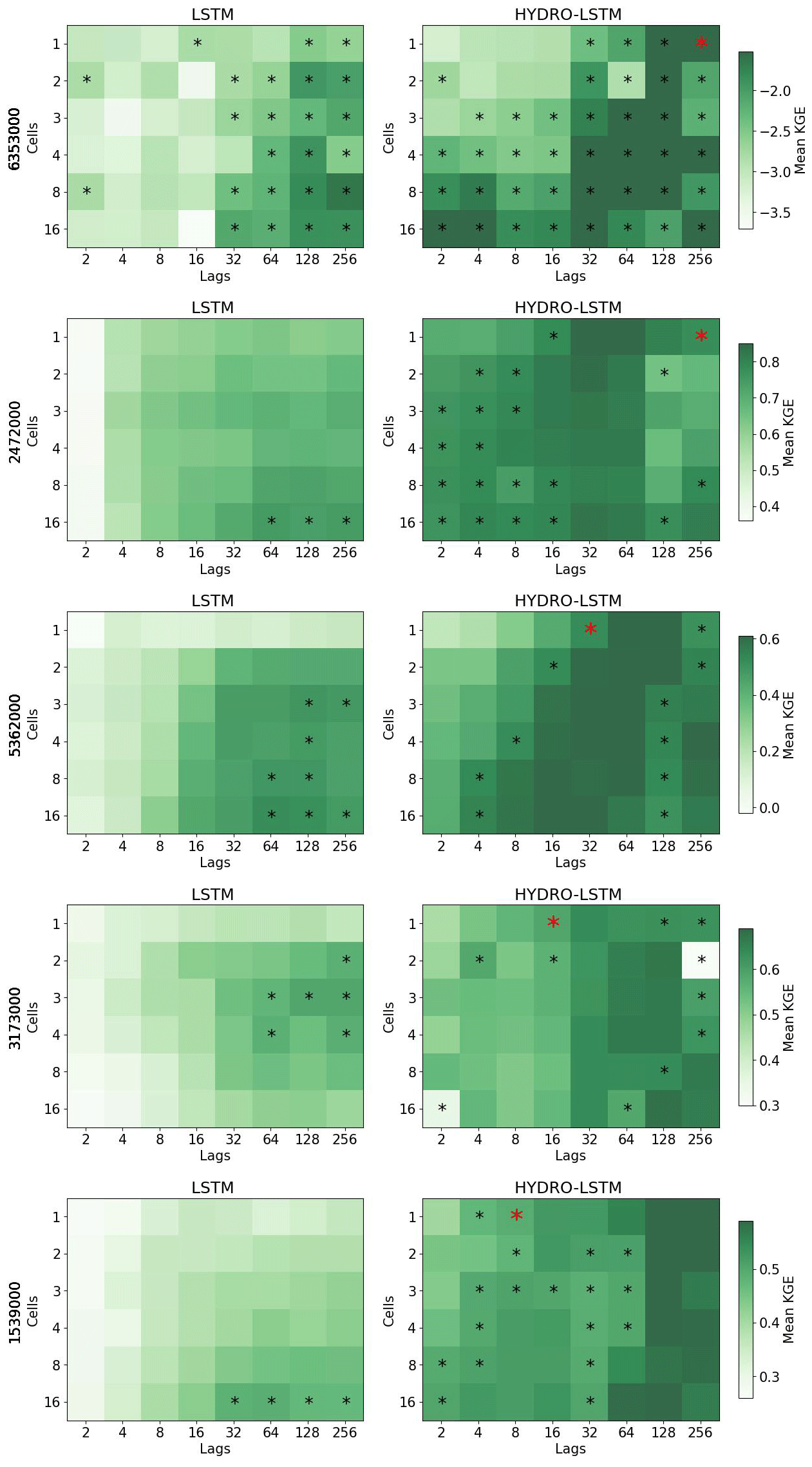
Figure A2Performance heatmap for different hyperparameter sets, number of cells, and lag days. Rows: Catchment studied. Columns: representation. An asterisk shows the hyperparameter sets with no statistical difference in the mean with respect to the red asterisk.
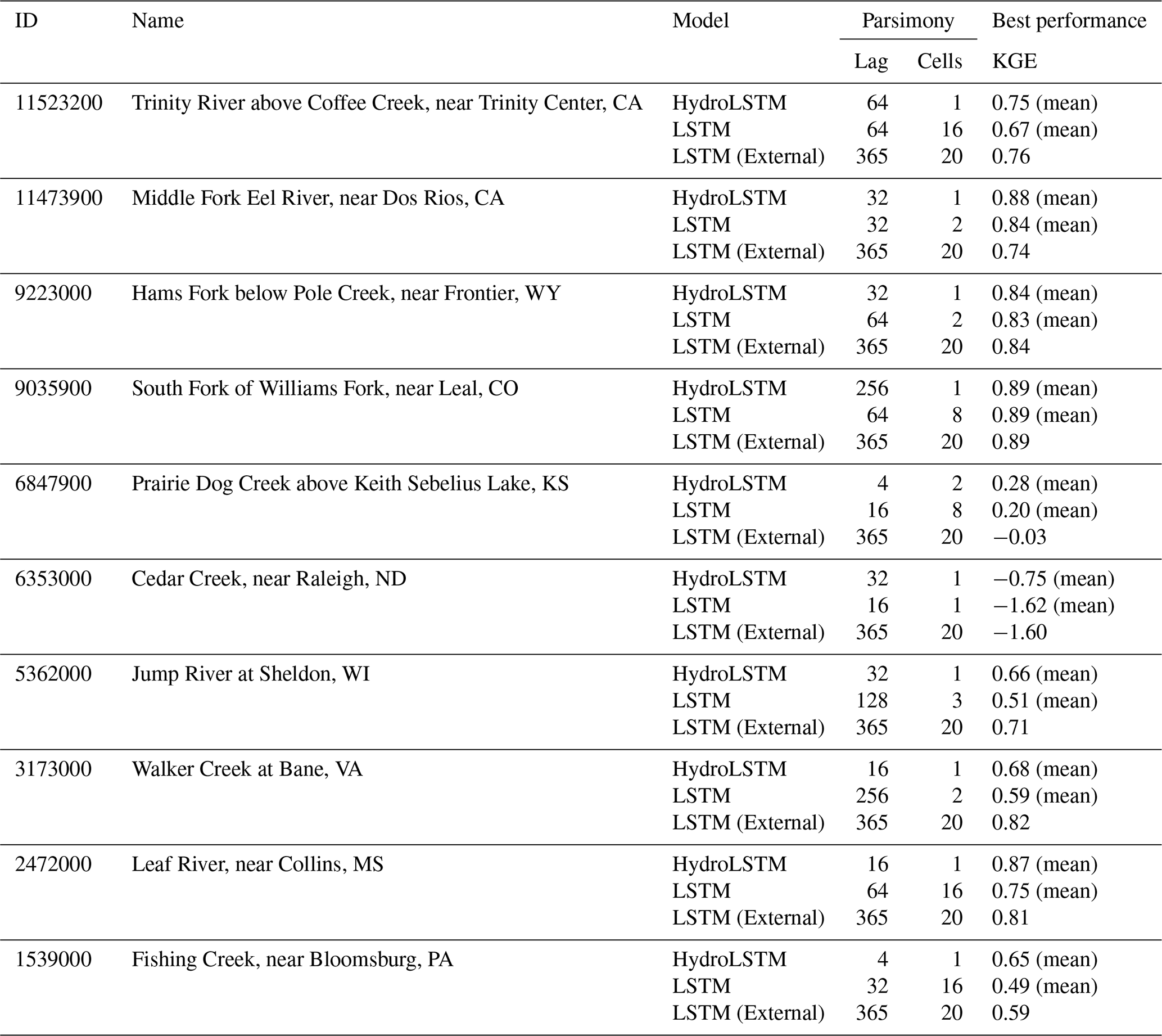
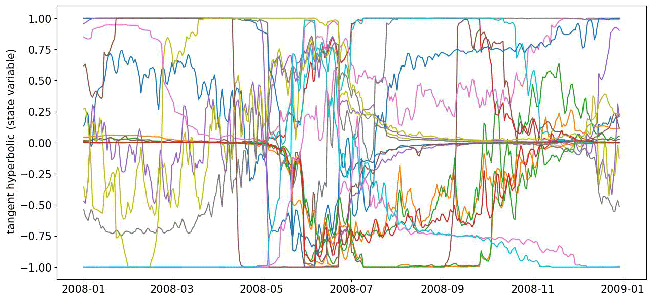
Figure B1Time evolution of the state variable across the ensemble of 20 models for the catchment South Fork of Williams Fork, CO. A unique evolution does not exist despite having good performance and one cell representation.
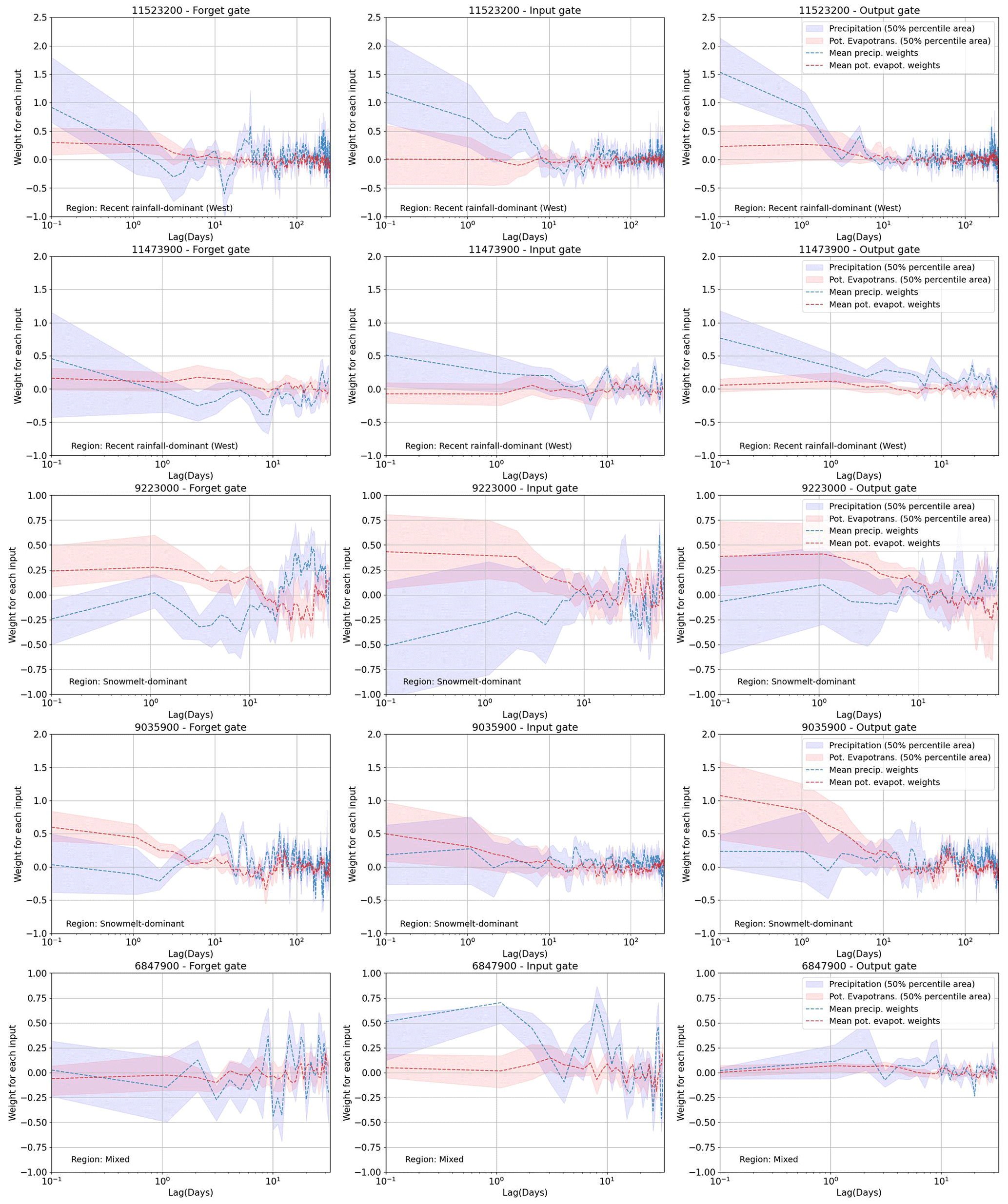
Figure C1Weight distribution in the three gates for HydroLSTM. Each row represents a different catchment. The confidence interval is the result of running 20 models with random initialization.
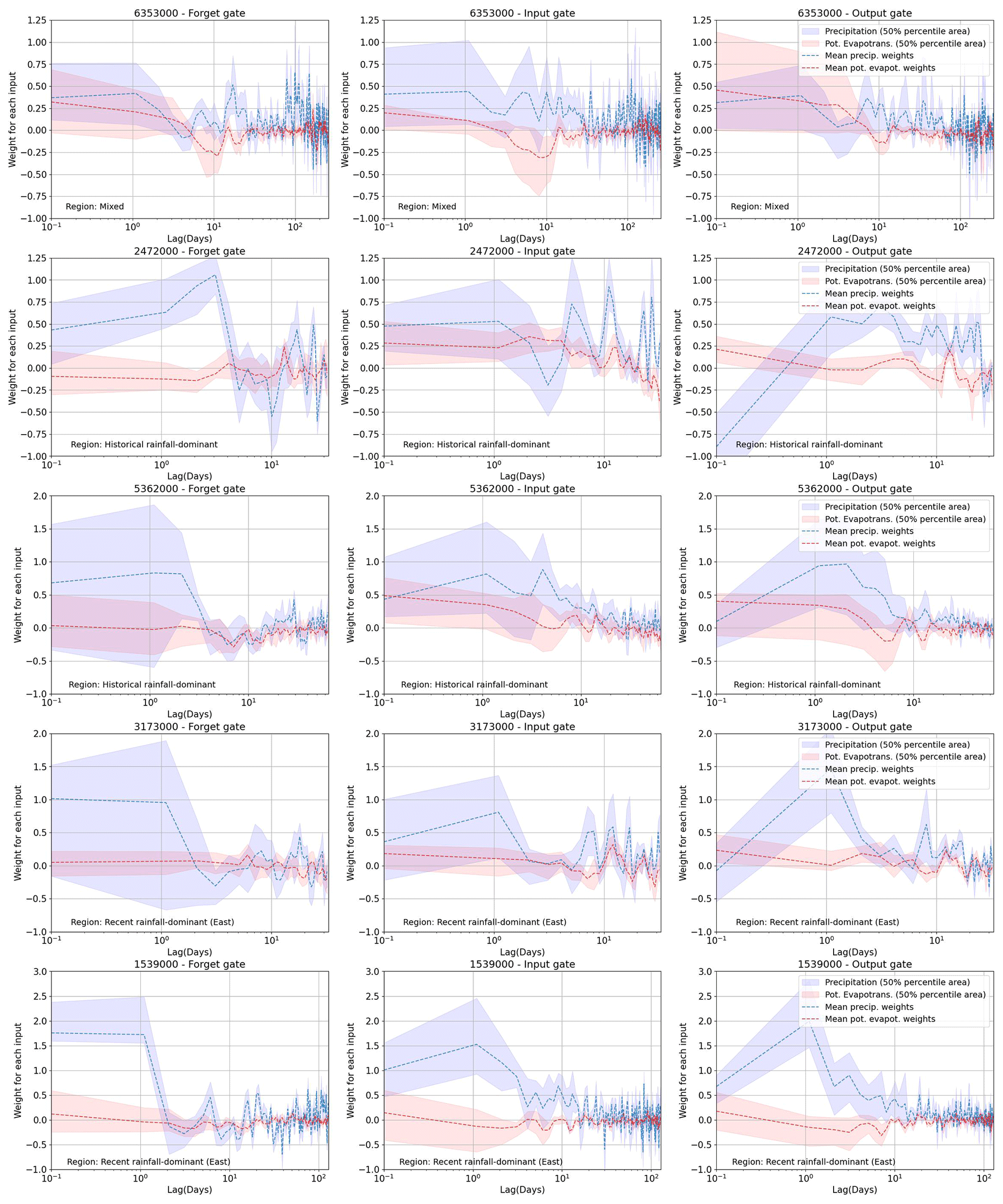
Figure C2Weight distribution in the three gates for HydroLSTM. Each row represents a different catchment. The confidence interval is the result of running 20 models with random initialization.
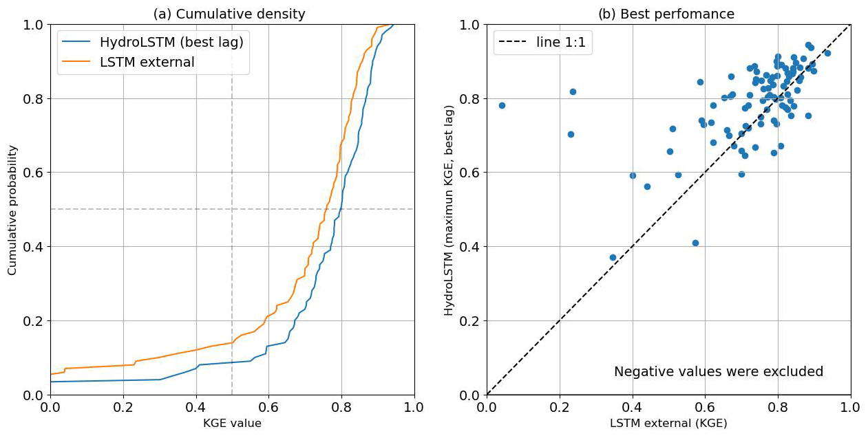
Figure D1Comparison of HydroLSTM and LSTM (external source) calibrated for 100 catchments independently (100 single models). (a) HydroLSTM using the best lag for each catchment has the potential to have an overall better performance than LSTM. (b) The scatter plot shows a trend around the line 1:1; however, there is no representation that outperforms the other in all the cases.
The codes to run the model and the Jupiter notebook used to create the figures are freely available at https://doi.org/10.5281/zenodo.10694927 (De la Fuente and Bennett, 2024).
The CAMELS dataset is freely available from https://doi.org/10.5065/D6MW2F4D (Newman et al., 2014).
The supplement related to this article is available online at: https://doi.org/10.5194/hess-28-945-2024-supplement.
LADlF, MRE, and HVG participated in the initial conceptualization. LADlF and MRE (early stage) developed the formal analysis. HVG nd LEC participated in the methodology and supervision. LADlF developed the original draft, with partial assistance from AI tools for checking grammar and fluency, and the entire team worked on reviewing and editing the document.
The contact author has declared that none of the authors has any competing interests.
Publisher's note: Copernicus Publications remains neutral with regard to jurisdictional claims made in the text, published maps, institutional affiliations, or any other geographical representation in this paper. While Copernicus Publications makes every effort to include appropriate place names, the final responsibility lies with the authors.
The authors would like to acknowledge the funding of NSF and ANID, and the feedback received from the CondonLab team and the reviewers.
This research has been supported by the Division of Earth Sciences (grant no. 1945195), the Innovation and Technology Ecosystems (grant no. 2134892), and the Comisión Nacional de Investigación Científica y Tecnológica (grant no. Becas Chile, 2022).
This paper was edited by Erwin Zehe and reviewed by Tadd Bindas and two anonymous referees.
Addor, N., Newman, A. J., Mizukami, N., and Clark, M. P.: The CAMELS data set: catchment attributes and meteorology for large-sample studies, Hydrol. Earth Syst. Sci., 21, 5293–5313, https://doi.org/10.5194/hess-21-5293-2017, 2017.
Addor, N., Nearing, G., Prieto, C., Newman, A. J., Le Vine, N., and Clark, M. P.: A Ranking of Hydrological Signatures Based on Their Predictability in Space, Water Resour. Res., 54, 8792–8812, https://doi.org/10.1029/2018WR022606, 2018.
Ali, G., Tetzlaff, D., Soulsby, C., McDonnell, J. J., and Capell, R.: A comparison of similarity indices for catchment classification using a cross-regional dataset, Adv. Water Resour., 40, 11–22, https://doi.org/10.1016/j.advwatres.2012.01.008, 2012.
Breiman, L.: Random Forest, Mach. Learn., 45, 5–32, https://doi.org/10.1023/A:1010933404324, 2001.
Burnash, R., Ferral, L., and McGuire, R.: A Generalized Streamflow Simulation System: Conceptual Modeling for Digital Computers, U.S. Department of Commerce, National Weather Service, and State of California, Department of Water Resources, 204 pp., https://www.google.com/books/edition/A_Generalized_Streamflow_Simulation_Syst/aQJDAAAAIAAJ?hl=en (last access: January 2023), 1973.
Carvalho, D. V., Pereira, E. M., and Cardoso, J. S.: Machine Learning Interpretability: A Survey on Methods and Metrics, Electronics, 8, 832, https://doi.org/10.3390/electronics8080832, 2019.
Chen, J., Zheng, F., May, R., Guo, D., Gupta, H., and Maier, H. R.: Improved data splitting methods for data-driven hydrological model development based on a large number of catchment samples, J. Hydrol., 613, 128340, https://doi.org/10.1016/j.jhydrol.2022.128340, 2022.
Cho, K. and Kim, Y.: Improving streamflow prediction in the WRF-Hydro model with LSTM networks, J. Hydrol., 605, 127297, https://doi.org/10.1016/j.jhydrol.2021.127297, 2022.
Cui, Z., Zhou, Y., Guo, S., Wang, J., Ba, H., and He, S.: A novel hybrid XAJ-LSTM model for multi-step-ahead flood forecasting, Hydrol. Res., 52, 1436–1454, https://doi.org/10.2166/nh.2021.016, 2021.
De la Fuente, L.: Using Big-Data to Develop Catchment-Scale Hydrological Models for Chile, University of Arizona, 123 pp., http://hdl.handle.net/10150/656824 (last access: January 2023), 2021.
De la Fuente, L. A. and Bennett, A.: ldelafue/Hydro-LSTM: HydroLSTM (v1.0.0), Zenodo [code], https://doi.org/10.5281/zenodo.10694927, 2024.
De la Fuente, L. A., Gupta, H. V., and Condon, L. E.: Toward a Multi-Representational Approach to Prediction and Understanding, in Support of Discovery in Hydrology, Water Resour. Res., 59, e2021WR031548, https://doi.org/10.1029/2021WR031548, 2023.
de Lavenne, A., Andréassian, V., Crochemore, L., Lindström, G., and Arheimer, B.: Quantifying multi-year hydrological memory with Catchment Forgetting Curves, Hydrol. Earth Syst. Sci., 26, 2715–2732, https://doi.org/10.5194/hess-26-2715-2022, 2022.
Erion, G., Janizek, J. D., Sturmfels, P., Lundberg, S. M., and Lee, S.-I.: Improving performance of deep learning models with axiomatic attribution priors and expected gradients, Nat. Mach. Intell., 3, 620–631, https://doi.org/10.1038/s42256-021-00343-w, 2021.
Fan, F., Xiong, J., Li, M., and Wang, G.: On Interpretability of Artificial Neural Networks: A Survey, arXiv [preprint], https://doi.org/10.48550/arXiv.2001.02522, 2020.
Friedman, J. H.: Greedy Function Approximation: A Gradient Boosting Machine, Ann. Stat., 29, 1189–1232, 2001.
Gauch, M., Mai, J., and Lin, J.: The proper care and feeding of CAMELS: How limited training data affects streamflow prediction, Environ. Modell. Softw., 135, 104926, https://doi.org/10.1016/j.envsoft.2020.104926, 2021.
Gers, F. A. and Schmidhuber, E.: LSTM recurrent networks learn simple context-free and context-sensitive languages, IEEE T. Neural Networ., 12, 1333–1340, https://doi.org/10.1109/72.963769, 2001.
Glorot, X. and Bengio, Y.: Understanding the difficulty of training deep feedforward neural networks, Proc. Mach. Learn. Res., 9, 249–256, 2010.
Graves, A., Eck, D., Beringer, N., and Schmidhuber, J.: Biologically Plausible Speech Recognition with LSTM Neural Nets, in: Biologically Inspired Approaches to Advanced Information Technology, vol. 3141, edited by: Ijspeert, A. J., Murata, M., and Wakamiya, N., Springer Berlin Heidelberg, Berlin, Heidelberg, 127–136, https://doi.org/10.1007/978-3-540-27835-1_10, 2004.
Guo, D., Zheng, F., Gupta, H., and Maier, H. R.: On the Robustness of Conceptual Rainfall-Runoff Models to Calibration and Evaluation Data Set Splits Selection: A Large Sample Investigation, Water Resour. Res., 56, e2019WR026752, https://doi.org/10.1029/2019WR026752, 2020.
Gupta, H. V., Kling, H., Yilmaz, K. K., and Martinez, G. F.: Decomposition of the mean squared error and NSE performance criteria: Implications for improving hydrological modelling, J. Hydrol., 377, 80–91, https://doi.org/10.1016/j.jhydrol.2009.08.003, 2009.
Hargreaves, G. and Samani, Z.: Reference Crop Evapotranspiration from Temperature, Appl. Eng. Agric., 1, 96–99, https://doi.org/10.13031/2013.26773, 1985.
Hey, T., Butler, K., Jackson, S., and Thiyagalingam, J.: Machine learning and big scientific data, Philos. T. Roy. Soc. A, 378, 20190054, https://doi.org/10.1098/rsta.2019.0054, 2020.
Hochreiter, S. and Schmidhuber, J.: Long Short-Term Memory, Neural Comput., 9, 1735–1780, https://doi.org/10.1162/neco.1997.9.8.1735, 1997.
Hoedt, P.-J., Kratzert, F., Klotz, D., Halmich, C., Holzleitner, M., Nearing, G., Hochreiter, S., and Klambauer, G.: MC-LSTM: Mass-Conserving LSTM, in: Volume 139: International Conference on Machine Learning, 18–24 July 2021, virtual, 4275–4286, https://proceedings.mlr.press/v139/hoedt21a.html (last access: January 2023), 2021.
Huber, P. J.: Robust Estimation of a Location Parameter, Ann. Math. Stat., 35, 73–101, https://doi.org/10.1214/aoms/1177703732, 1964.
Jiang, S., Zheng, Y., Wang, C., and Babovic, V.: Uncovering Flooding Mechanisms Across the Contiguous United States Through Interpretive Deep Learning on Representative Catchments, Water Resour. Res., 58, e2021WR030185, https://doi.org/10.1029/2021WR030185, 2022.
Khandelwal, A., Xu, S., Li, X., Jia, X., Stienbach, M., Duffy, C., Nieber, J., and Kumar, V.: Physics Guided Machine Learning Methods for Hydrology, arXiv [preprint], https://doi.org/10.48550/arXiv.2012.02854, 2020.
Kingma, D. P. and Ba, J.: Adam: A Method for Stochastic Optimization, arXiv [preprint], https://doi.org/10.48550/arXiv.1412.6980, 29 January 2017.
Kratzert, F., Klotz, D., Brenner, C., Schulz, K., and Herrnegger, M.: Rainfall–runoff modelling using Long Short-Term Memory (LSTM) networks, Hydrol. Earth Syst. Sci., 22, 6005–6022, https://doi.org/10.5194/hess-22-6005-2018, 2018.
Kratzert, F., Klotz, D., Shalev, G., Klambauer, G., Hochreiter, S., and Nearing, G.: Towards learning universal, regional, and local hydrological behaviors via machine learning applied to large-sample datasets, Hydrol. Earth Syst. Sci., 23, 5089–5110, https://doi.org/10.5194/hess-23-5089-2019, 2019.
Kratzert, F., Gauch, M., Nearing, G., and Klotz, D.: NeuralHydrology – A Python library for Deep Learningresearch in hydrology, J. Open Sour. Softw., 7, 4050, https://doi.org/10.21105/joss.04050, 2022.
Lees, T., Reece, S., Kratzert, F., Klotz, D., Gauch, M., De Bruijn, J., Kumar Sahu, R., Greve, P., Slater, L., and Dadson, S. J.: Hydrological concept formation inside long short-term memory (LSTM) networks, Hydrol. Earth Syst. Sci., 26, 3079–3101, https://doi.org/10.5194/hess-26-3079-2022, 2022.
Lienhard, J. H.: A statistical mechanical prediction of the dimensionless unit hydrograph, J. Geophys. Res., 69, 5231–5238, https://doi.org/10.1029/JZ069i024p05231, 1964.
Linardatos, P., Papastefanopoulos, V., and Kotsiantis, S.: Explainable AI: A Review of Machine Learning Interpretability Methods, Entropy, 23, 18, https://doi.org/10.3390/e23010018, 2020.
Ma, Y., Montzka, C., Bayat, B., and Kollet, S.: Using Long Short-Term Memory networks to connect water table depth anomalies to precipitation anomalies over Europe, Hydrol. Earth Syst. Sci., 25, 3555–3575, https://doi.org/10.5194/hess-25-3555-2021, 2021.
Miller, T.: Explanation in artificial intelligence: Insights from the social sciences, Artif. Intell., 267, 1–38, https://doi.org/10.1016/j.artint.2018.07.007, 2019.
Molnar, C.: Interpretable Machine Learning, 2nd Edn., Independently, https://christophm.github.io/interpretable-ml-book/ (last access: January 2023), 2022.
Newman, A., Sampson, K., Clark, M., Bock, A., Viger, R., Blodgett, D., Addor, N., and MIzukami, M.: A large-sample watershed-scale hydrometeorological dataset for the contiguous USA, NCAR [data set], https://doi.org/10.5065/D6MW2F4D, 2014.
Parviainen, E.: Dimension Reduction for Regression with Bottleneck Neural Networks, in: Intelligent Data Engineering and Automated Learning – IDEAL 2010, vol. 6283, edited by: Fyfe, C., Tino, P., Charles, D., Garcia-Osorio, C., and Yin, H., Springer Berlin Heidelberg, Berlin, Heidelberg, 37–44, https://doi.org/10.1007/978-3-642-15381-5_5, 2010.
Perrin, C., Michel, C., and Andréassian, V.: Improvement of a parsimonious model for streamflow simulation, J. Hydrol., 279, 275–289, https://doi.org/10.1016/S0022-1694(03)00225-7, 2003.
Pilgrim, D. H., Chapman, T. G., and Doran, D. G.: Problems of rainfall-runoff modelling in arid and semiarid regions, Hydrolog. Sci. J., 33, 379–400, https://doi.org/10.1080/02626668809491261, 1988.
Pugliese, R., Regondi, S., and Marini, R.: Machine learning-based approach: global trends, research directions, and regulatory standpoints, Data Science and Management, 4, 19–29, https://doi.org/10.1016/j.dsm.2021.12.002, 2021.
Qiu, R., Wang, Y., Rhoads, B., Wang, D., Qiu, W., Tao, Y., and Wu, J.: River water temperature forecasting using a deep learning method, J. Hydrol., 595, 126016, https://doi.org/10.1016/j.jhydrol.2021.126016, 2021.
Rodríguez-Iturbe, I. and Valdés, J. B.: The geomorphologic structure of hydrologic response, Water Resour. Res., 15, 1409–1420, https://doi.org/10.1029/WR015i006p01409, 1979.
Sherman, L.: Stream Flow from Rainfall by the Unit Graph Method, Eng. News-Rec., 108, 501–505, 1932.
Singh, R., Archfield, S. A., and Wagener, T.: Identifying dominant controls on hydrologic parameter transfer from gauged to ungauged catchments – A comparative hydrology approach, J. Hydrol., 517, 985–996, https://doi.org/10.1016/j.jhydrol.2014.06.030, 2014.
Song, H., Kim, S., Kim, M., and Lee, J.-G.: Ada-boundary: accelerating DNN training via adaptive boundary batch selection, Mach. Learn., 109, 1837–1853, https://doi.org/10.1007/s10994-020-05903-6, 2020.
Vaswani, A., Shazeer, N., Parmar, N., Uszkoreit, J., Jones, L., Gomez, A. N., Kaiser, L., and Polosukhin, I.: Attention Is All You Need, arXiv [preprint], https://doi.org/10.48550/arXiv.1706.03762, 2017.
Wang, Y., Gupta, H. V., Zeng, X., and Niu, G.: Exploring the Potential of Long Short-Term Memory Networks for Improving Understanding of Continental- and Regional-Scale Snowpack Dynamics, Water Resour. Res., 58, e2021WR031033, https://doi.org/10.1029/2021WR031033, 2022.
Xu, T. and Liang, F.: Machine learning for hydrologic sciences: An introductory overview, WIREs Water, 8, e1533, https://doi.org/10.1002/wat2.1533, 2021.
Zheng, F., Maier, H. R., Wu, W., Dandy, G. C., Gupta, H. V., and Zhang, T.: On Lack of Robustness in Hydrological Model Development Due to Absence of Guidelines for Selecting Calibration and Evaluation Data: Demonstration for Data-Driven Models, Water Resour. Res., 54, 1013–1030, https://doi.org/10.1002/2017WR021470, 2018.
Zheng, F., Chen, J., Maier, H. R., and Gupta, H.: Achieving Robust and Transferable Performance for Conservation-Based Models of Dynamical Physical Systems, Water Resour. Res., 58, e2021WR031818, https://doi.org/10.1029/2021WR031818, 2022.
- Abstract
- Introduction
- Structural analysis of LSTM
- Proposed HydroLSTM structure
- Methods
- First experiment: comparison of both representations
- Second experiment: learning from many catchments
- Discussion
- Conclusions
- Appendix A: Comparison between LSTM and HydroLSTM for all the catchments
- Appendix B: Summary of the comparison between LSTM and HydroLSTM (first dataset)
- Appendix C: Weight distribution for the 10 catchments
- Appendix D: Broader comparison between HydroLSTM and LSTM
- Code availability
- Data availability
- Author contributions
- Competing interests
- Disclaimer
- Acknowledgements
- Financial support
- Review statement
- References
- Supplement