Current and future roles of meltwater–groundwater dynamics in a proglacial Alpine outwash plain

Glacierized alpine catchments are rapidly evolving due to glacier retreat and consequent geomorphological and ecological changes. As more terrain becomes ice-free, reworking of exposed terrain by the river as well as thawing of the top layer may lead to an increase in surface and subsurface water exchanges, leading to potential changes in water storage and release, which in turn may impact ecological, geomorphological and hydrological processes. In this study, we aim to understand the current and future hydrological functioning of a typical outwash plain in a Swiss Alpine catchment. As with many other fluvial aquifers in alpine environments, this outwash plain is located at the valley bottom, where catchment-wide water and sediment fluxes tend to gather from multiple sources, may store water and provide specific habitats for alpine ecosystems. Their dynamics are however rarely studied in post Little Ice Age proglacial zones. Based on geophysical investigations as well as year-round stream and groundwater observations, we developed a simplified physically based 3D MODFLOW model and performed an optimized automatic calibration using PEST HP. We highlight the strong interactions between the upstream river and the aquifer, with stream infiltration being the dominant process of recharge. Groundwater exfiltration occurs in the lower half of the outwash plain, balancing out the amount of river infiltration at a daily timescale. We show that hillslope contributions from rain and snowmelt have little impact on groundwater levels. We also show that the outwash plain acts as a bedrock-dammed aquifer and can maintain groundwater levels close to the surface during dry periods lasting months, even in the absence of glacier meltwater, but may in turn provide only limited baseflow to the stream. Finally, we explore how new outwash plains may form in the future in this catchment due to glacier recession and discuss from a hydrological perspective which cascading impacts the presence of multiple outwash plains may have. For this case study, we estimate the total dynamic storage of future outwash plains to be about 20 mm, and we demonstrate their limited capacity to provide more stream water than that which they infiltrate upstream, except for very low river flows (<150 to 200 L s⁻¹). Below this limit, they can provide limited baseflow on timescales of weeks, thus maintaining moisture conditions that may be beneficial for proglacial ecosystems. Their role in attenuating floods also appears limited, as less than 0.5 m³ s⁻¹ of river water can be infiltrated. The studied outwash plain appears therefore to play an important role for alpine ecosystems but has a marginal hydrological effect on downstream river discharge.

1 Introduction

Alpine glacierized catchments are rapidly evolving under the effect of rising temperatures and rapid glacier melt. Previously ice-covered glacial forefields may be impacted by substantial sediment release from glacierized and deglacierized hillslopes (Mancini and Lane, 2020) as well as reworking by glacier meltwater (Carrivick and Heckmann, 2017), leading to rapid geomorphological and ecological changes. In addition, seasonal water supply is changing, with more winter liquid precipitation, earlier snowmelt and ice melt, more intense diurnal discharge cycles and reduced snowmelt supply in the later summer months (Berghuijs et al., 2014; Milner et al., 2017; Lane and Nienow, 2019). These combined climatic, hydrological and geomorphological processes are strongly modifying the hydrology of glacierized catchments, which may have implications for high-elevation hydropower production (Schaefli et al., 2019), water-related hazards, proglacial and regional ecology (Brighenti et al., 2019b) and downstream water availability.

In this context, research has focused on characterizing the influence of glacier retreat on the geomorphological processes influencing sediment transport (Lane et al., 2017) and on the evolution of seasonal streamflow volumes (e.g. Huss et al., 2008; Huss and Hock, 2018). However, assessment of the role of groundwater storage and release is usually oversimplified (Vincent et al., 2019), even if it may play an important role, especially during extreme drought events (Buytaert et al., 2017). Due to the complexity of landforms in glacial forefields and their susceptibility to rapid reworking, groundwater storage is likely contained in different compartments such as superficial landforms or bedrock fractures with different water storage potential and retention timescales (Hayashi, 2020; Müller et al., 2022). For this reason, a sound understanding of future water availability and storage in alpine glacierized catchments can only be achieved by acquiring detailed knowledge of the hydrological functioning of different landforms and their associated water storage potential as well as of spatial groundwater recharge and exfiltration patterns (Müller et al., 2022). Some recent studies started to address this issue (Glas et al., 2018; Hayashi, 2020) by characterizing and mapping geomorphological landforms such as talus slopes (Muir et al., 2011; Kurylyk and Hayashi, 2017), lateral deposits (Baraer et al., 2015), moraines (Kobierska et al., 2015a; Langston et al., 2013; McClymont et al., 2011) or rock glaciers (Winkler et al., 2016; Wagner et al., 2021; Harrington et al., 2018). For a detailed review, the reader is referred to the work of Hayashi (2020).

Outwash plains have been less studied, and so here we characterize the hydrological behaviour of an alpine proglacial outwash plain, a type of newly formed fluvial aquifer composed of gravelly–sandy sediments deposited in front of a glacier after subglacial erosion (Ballantyne, 2002). Those landforms mainly form in glacier forefields where sediment supply from glacial erosion and rock-slope failure is substantial and in locations where the valley bottom is characterized by a low slope, where sediment deposition can occur (Maizels, 2002). The ecological importance of older Quaternary fluvial deposits has been studied, showing that their location in flat valley bottoms allows them to accumulate water, sediments and organic matter from different sources, leading to a patchwork of environmental habitats essential for endemic species (Hauer et al., 2016; Crossman et al., 2011; Miller and Lane, 2018). Studies have shown strong surface water–groundwater interactions with infiltrated stream water extending hundreds of metres laterally beyond the stream network (Ó Dochartaigh et al., 2019; Hauer et al., 2016) and with a dominant longitudinal groundwater gradient, which leads to groundwater upwelling in downstream river sections (Ward et al., 1999). Whilst the behaviour of such larger aquifers is well known, the emergence of new small alluvial floodplains after the Little Ice Age (LIA) in the Alps has not been studied from a hydrological perspective, with the exception of a series of studies in Val Roseg in the Swiss Alps (Ward et al., 1999; Malard et al., 1999). Fluvial landforms in post-LIA proglacial zones have been shown to represent less than 5 % of the area of deglaciated terrain in the European Alps (Carrivick et al., 2018), but their proportion may increase rapidly with the retreat of the glacier tongues which often occupy the flatter part of alpine catchments.

The importance of further research in this field is emphasized by the fact that proglacial outwash plains will likely provide the only viable habitat for cold-water species (Brighenti et al., 2019b) and may store relatively large amounts of water. Four questions arise. (i) What are their future spatial extent and hydrological significance in deglacierized terrain? (ii) Are their groundwater dynamics similar to larger Quaternary floodplains in terms of their potential to maintain shallow groundwater seasonally? (iii) How will they respond to early season and reduced ice melt and snowmelt? (iv) How will vegetation feedbacks influence their stability and water and sediment storage (Roncoroni et al., 2019)?

We address the first three questions by providing a detailed analysis of a selected case study in the Swiss Alps, the Otemma Glacier forefield, where a large outwash plain system has been monitored for sediment, ecological and hydrological processes since 2019 (Müller et al., 2022). Based on 2 years of groundwater well observations and discharge and electrical conductivity measurements, we build a 3D MODFLOW model to characterize the groundwater dynamics and the rate of stream water infiltration and groundwater exfiltration. This allows us to characterize the surface water–groundwater dynamics of a typical outwash plain, which is likely similar to those of other alpine environments. Finally, we apply the developed model to a hypothetical future scenario where new outwash plains are formed due to glacier retreat in deglacierized bedrock overdeepenings and demonstrate their overall hydrological significance.

2 Study site and experimental methods

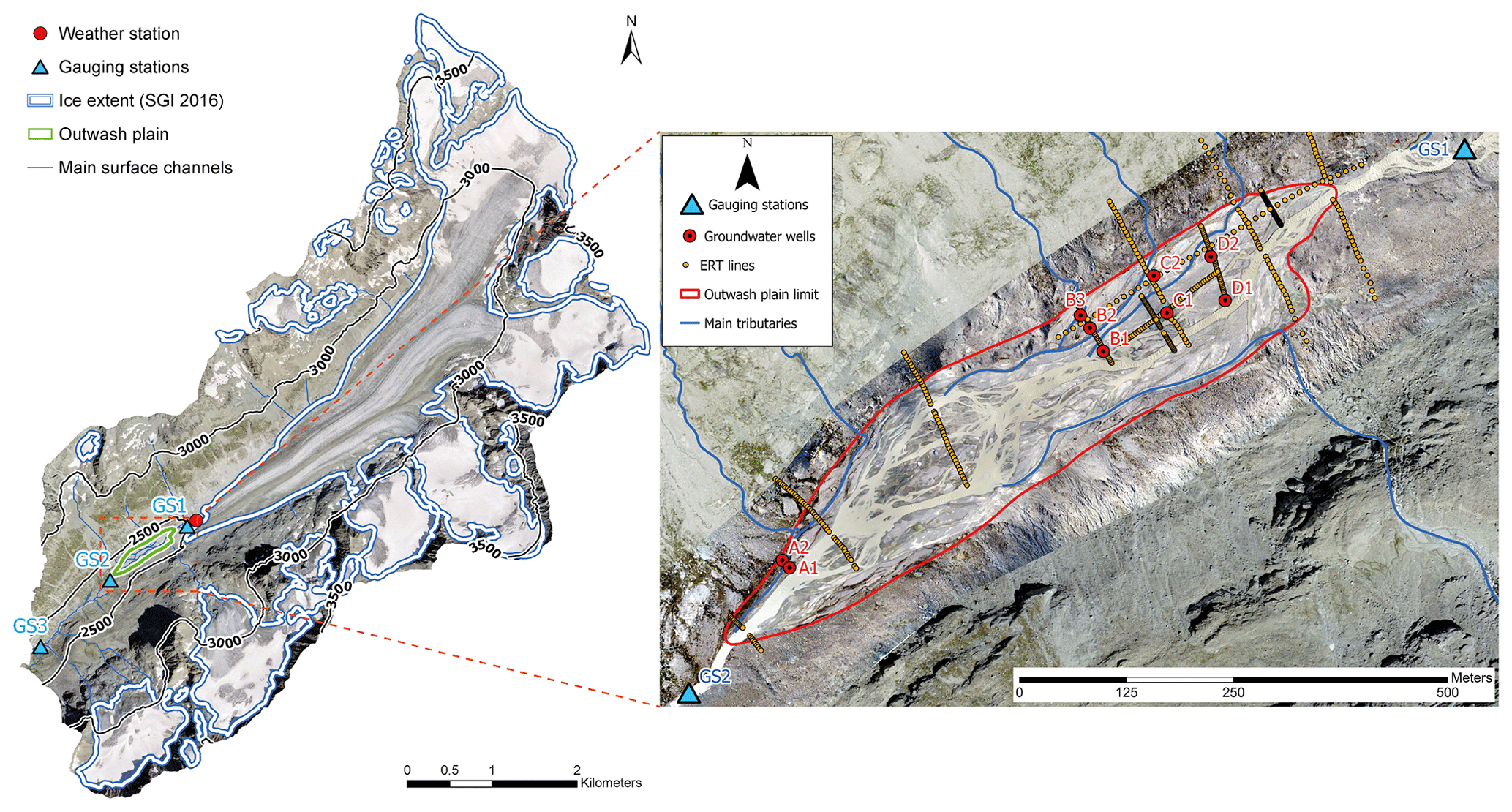
The Otemma Glacier is located in the western Swiss Alps (45^∘56^′03^′′ N, 7^∘24^′42^′′ E) with a catchment area of 30.3 km², a mean elevation of 3005 m a.s.l. (2350 to 3780 m a.s.l.) and about 45 % glacier cover in 2020 (Linsbauer et al., 2021). The glacier is characterized by a relatively flat tongue which is rapidly retreating. The outwash plain studied here was gradually uncovered between 1988 and 2020 over a length of about 1250 m in 32 years or a glacier retreat rate of almost 40 m yr⁻¹ (GLAMOS, 1881–2020).

The underlying bedrock consists of orthogneiss and metagranodiorites (Burri et al., 1999), overlain by coarse superficial sediment deposits with limited vegetation development and shallow, young soils. The outwash plain is composed of non-consolidated sandy–gravelly material forming a mosaic of bars and terraces. It covers a surface of 118 000 m² or 0.4 % of the total catchment area. The main stream network is braided in the lower part of the plain, with rapid channel modifications due to periodic high discharge, and is more constrained in the upper part, where the stream is usually limited to one channel, although large channel erosion (>5 m h⁻¹ laterally) was also observed during large flood events (once a year). There is a general downslope gradient from coarser to finer sandy–silty material typical of outwash plains (Zielinski and Van Loon, 2003; Maizels, 2002). Melt-out of buried ice is also observed, leading to the formation of “kettle holes” (Maizels, 1977). The outwash plain has a longitudinal length of about 900 m and a slope between 1 % in its lower part and 2 % upstream as well as a mean slope of 1.4 %. The lateral relief is variable between 2 and 3 m and is associated with terraces.

2.1 Meteorological data

Since 2019, a meteorological station has been installed near the glacier terminus at an elevation of 2450 m a.s.l. and has continuously measured liquid precipitation with a Davis tipping rain gauge as well as air temperature, relative humidity and pressure with a Decagon VP-4.

Additionally, winter solid precipitation was measured using the closest SwissMetNet weather station, either in Otemma (2357 m a.s.l.) or in Arolla (2005 m a.s.l.) for time steps where the Otemma station showed missing values (the two stations are 1.5 and 11.5 km from the outwash plain). The data acquired for this study and their description are available on Zenodo (Müller, 2022a).

2.2 Surface water data

Two gauging stations were installed in the main stream, upstream (GS1, Fig. 1) and downstream (GS2, Fig. 1) of the outwash plain in bedrock-constrained river sections. Stream temperature, water electrical conductivity (EC) and river stage were measured continuously at 10 min intervals using an automatic sensor (Keller DCX-22AA-CTD). Sensor measurements were checked against bi-monthly manual measurements. Discharge was estimated at both sites by building a stage–discharge rating curve. Point discharge measurements were performed by dilution gauging using fluorescence dye tracing (Rhodamine WT 20 %). The dye concentration was measured with a fluorometer (Albillia GGUN-FL30) recording at 5 s intervals following dye injection. For flows smaller than 1 m³ s⁻¹, discharge was measured using salt dilution gauging instead of dye. Dissolved salt concentration was measured using EC, and a local EC–salt concentration curve was built. In total, 27 discharge measurements were performed for GS1 and 21 for GS2 in 2020, together with 15 and 13 respectively in 2021. For each gauging station, we covered a wide range of discharge values, from low winter baseflow (100 L s⁻¹) to summer high flow (10 m³ s⁻¹). The estimated mean discharge uncertainty (95 % confidence) is 0.55 m³ s⁻¹. A more detailed description of the data is available in the work of Müller and Miesen (2022).

Figure 1 Overview of the Otemma catchment, the outwash plain and the gauging and weather stations. The window on the right shows the braided outwash plain with the eight groundwater wells and the main hillslope tributaries. The orthoimage was provided by SwissTopo (2020).

Along-stream gauging was also attempted to quantify rates of surface water–groundwater interactions. This was however only successful during the autumn period when streamflow is low and less turbulent, and thus streamflow measurements via salt gauging were more precise. This was the only period when the discharge measurement error was smaller than the water exchange rates. On 17 September 2021, we gauged the stream at three locations: above the start of the outwash plain (GS1), at the location of well B1 and at the end of the outwash plain (100 m above GS2). At that time, all surface tributaries were visually dry, so that lateral water inputs are negligible.

In addition to the main stream, small hillslope tributaries were also manually monitored for EC and water temperature. All manual measurements in this study were performed with the same device (WTW Multi 3510 IDS logger with a IDS TetraCon^® 925 water conductivity probe).

2.3 Groundwater measurements

Between 2019 and 2022 we installed eight fully screened groundwater observation wells in stable terraces of the outwash plain, consisting of three lateral transects (transects B, C and D) in the upstream part of the plain and one single well (A1) in the downstream part (Fig. 1). The wells reached a depth of about 2 m below the ground surface. Groundwater levels were measured using autonomous loggers (Seeeduino Stalker V3.1) equipped with SparkFun MS5803-14BA pressure sensors measuring at a 10 min interval. The sensor resolution was 1 mm with an accuracy of ±2 cm, and sensor bias was manually checked bi-monthly using manual groundwater stage measurements. The sensors functioned year-round, but the groundwater stage usually fell below the sensor in winter and sometimes the sensors were damaged by winter snow accumulation. A more detailed description of the data is available in the work of Müller (2022b). Periodic point measurements of groundwater EC and temperature were also performed. Prior to measurement, groundwater wells were flushed by pumping 3 times their water volumes.

The aquifer porosity was estimated by measuring the saturated water content (Decagon 5TM) at five random locations in the first metre of saturated sediments in the outwash plain. The surface sediment texture appeared visually relatively homogeneous except on slightly more elevated terraces on the side of the outwash plain where early signs of vegetation appeared. There, the finer soil texture was measured by laser granulometry (Beckmann Coulter grain sizer).

2.4 Electrical resistivity tomography

Electrical resistivity tomography (ERT) was performed in the outwash plain in order to map sediment depth and the underlying bedrock geometry with a Syscal Pro Switch 48 from Iris Instruments. The array consisted of 48 electrodes with a spacing between 1.5 and 4 m, and we performed both dipole–dipole (DD) and Wenner–Schlumberger (WS) schemes for each measurement site. The location of each electrode was measured with a GNSS GPS (Trimble R10 GNSS), and we performed 2D data inversion using the open-source pyGIMLi Python library (Rücker et al., 2017). We included topography and used a robust inversion scheme (L1-norm) with a set of regularization parameters in order to assess the results' sensitivity to over-fitting.

A total of 12 different electrical resistivity tomography profiles were obtained between 2019 and 2021. The depth of the sediments was identified based on a sharp transition from water-saturated sediments with resistivity values between 500 and 2000 Ωm to a lower layer with resistivity of between 4000 and 7000 Ωm. The depth profiles obtained with both electrode setups (DD and WS) were systematically compared to check the data quality acquired. Generally, both setups led to similar bedrock depths, but the results from the DD scheme were used as they usually led to a better vertical resolution.

Some more resistive patches were identified, with values larger than 10 000 Ωm, which we attributed to the presence of buried ice (Bosson et al., 2015). A more detailed description of the data is available in the work of Müller (2022c).

3 Methods

3.1 Three-dimensional MODFLOW model

We set up a 3D MODFLOW model of the outwash plain aquifer using the Python package Flopy (Bakker et al., 2016) with the latest MODFLOW 6.3 version (Langevin et al., 2022). The model was first initialized with a pre-defined set of parameters and, in a second phase, we calibrated the model parameters (Sect. 3.2.3) using the PEST HP optimization algorithm, a PEST version (Doherty, 2015) optimized for highly parallelized (HP) environments.

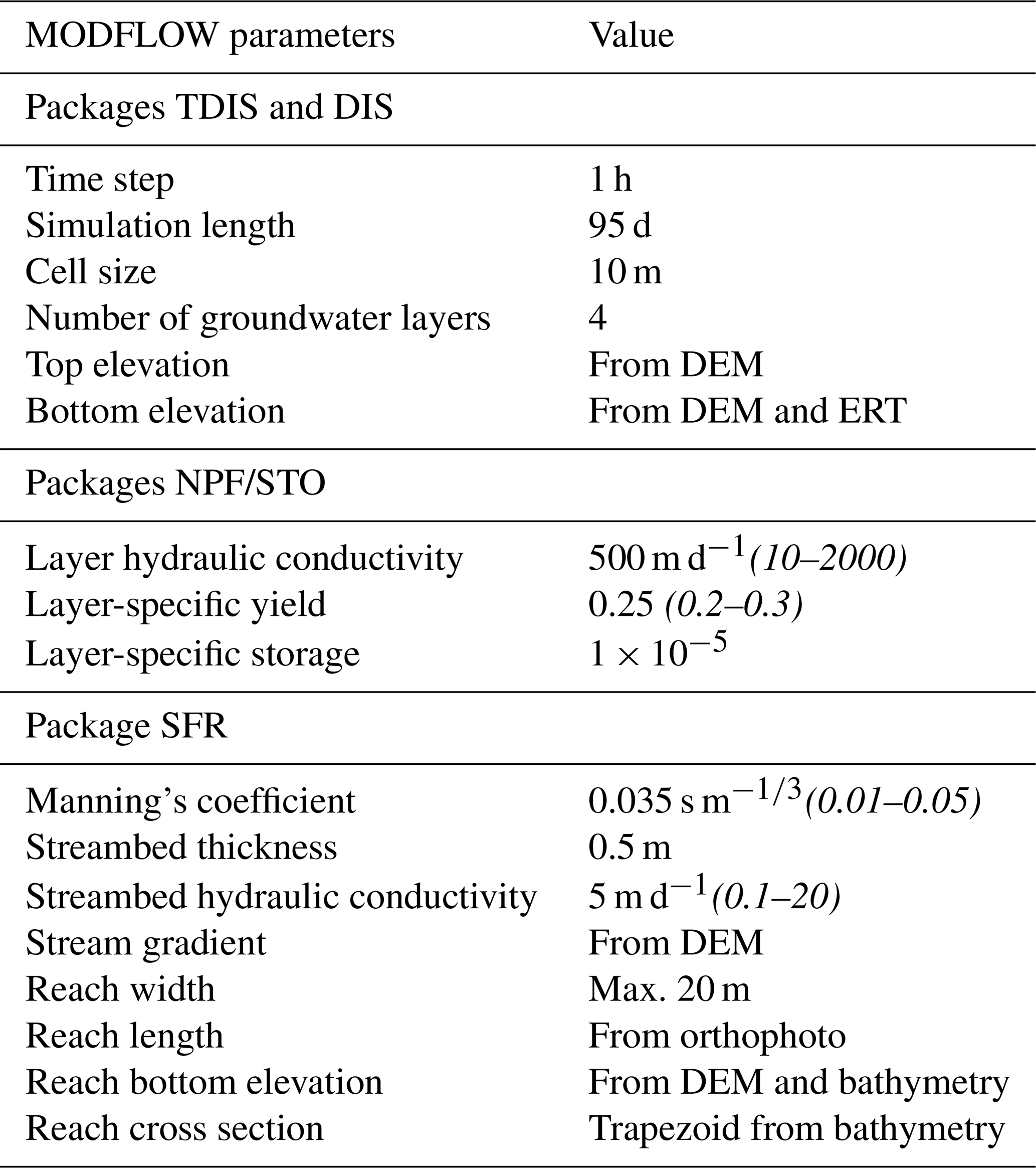
The calibrated model was then used to analyse the aquifer behaviour during an entire year. The main packages used to build the MODFLOW model are described in the following sections, and the main parameter values are summarized in Table 1.

Table 1 Summary of the main MODFLOW parameters by packages. Ranges in italics indicate bounds for parameters calibrated during the calibration phase.

3.1.1 Temporal discretization (TDIS)

The model is defined with an hourly time step. The time period for the calibration phase is from 15 August to 18 November 2020. This time period was considered adequate to cover both summer high flows and the autumn recession period.

3.1.2 Structured discretization (DIS), node property flow (NPF) and storage (STO)

The model lateral no-flow boundary corresponds to the limit of the outwash plain, which was manually digitized (Fig. 1). The surface topography was determined using surface-from-motion multi-view stereo (SfM-MVS) photogrammetry using imagery acquired with a Dji Phantom Drone, resulting in a final DEM with 0.25 m resolution and ±0.02 m precision. A detailed description of the procedure is provided in Roncoroni et al. (2022).

The DEM was then resampled to a model grid of 10 m by 10 m. In order to estimate the elevations of the water bodies precisely, we isolated the zones in the DEM corresponding to the stream network and performed a separate resampling of these zones only. Due to the typically larger noise in the DEM of the water bodies, we then applied a smoothing filter algorithm (Savitzky–Golay) along the stream network.

The depth of the model is defined using data from the ERT measurements. We only simulated the coarse-grained sediment aquifer and defined the underlying bedrock as the no-flow model boundary. We thus neglected any infiltration into the bedrock because its hydraulic conductivity is likely 3 to 4 orders of magnitude smaller (Masset and Loew, 2010) and is thus negligible for the timescales and purposes of our model. From the ERT transects, we manually drew lines of equal depth below the surface and then performed a spatial interpolation (Topo to Raster functions from ArcGIS) to create the bedrock topography of the whole domain (Fig. 2). The model domain is further split into four aquifer layers where hydraulic conductivity and porosity (specific yield) are allowed to vary spatially and independently of each layer. The unconfined aquifer is simply separated into four parts to allow parameters to vary with depth, and no layer is confined. Those parameters were calibrated in a second step using PEST HP (Sect. 3.2). The top layer includes the first 2 m below a sloping plane corresponding roughly to the elevation of the contour of the outwash plain to the top of the DEM. The next lower layer extends from −2 to −6 m, then from −6 to −10 m, and finally from −10 m to the depth of the bedrock (see Fig. 9 for an illustration). This partitioning was selected as a trade-off between allowing substantial parameter variation with depth and limiting the number of calibration layers (and parameters) which increased computational costs.

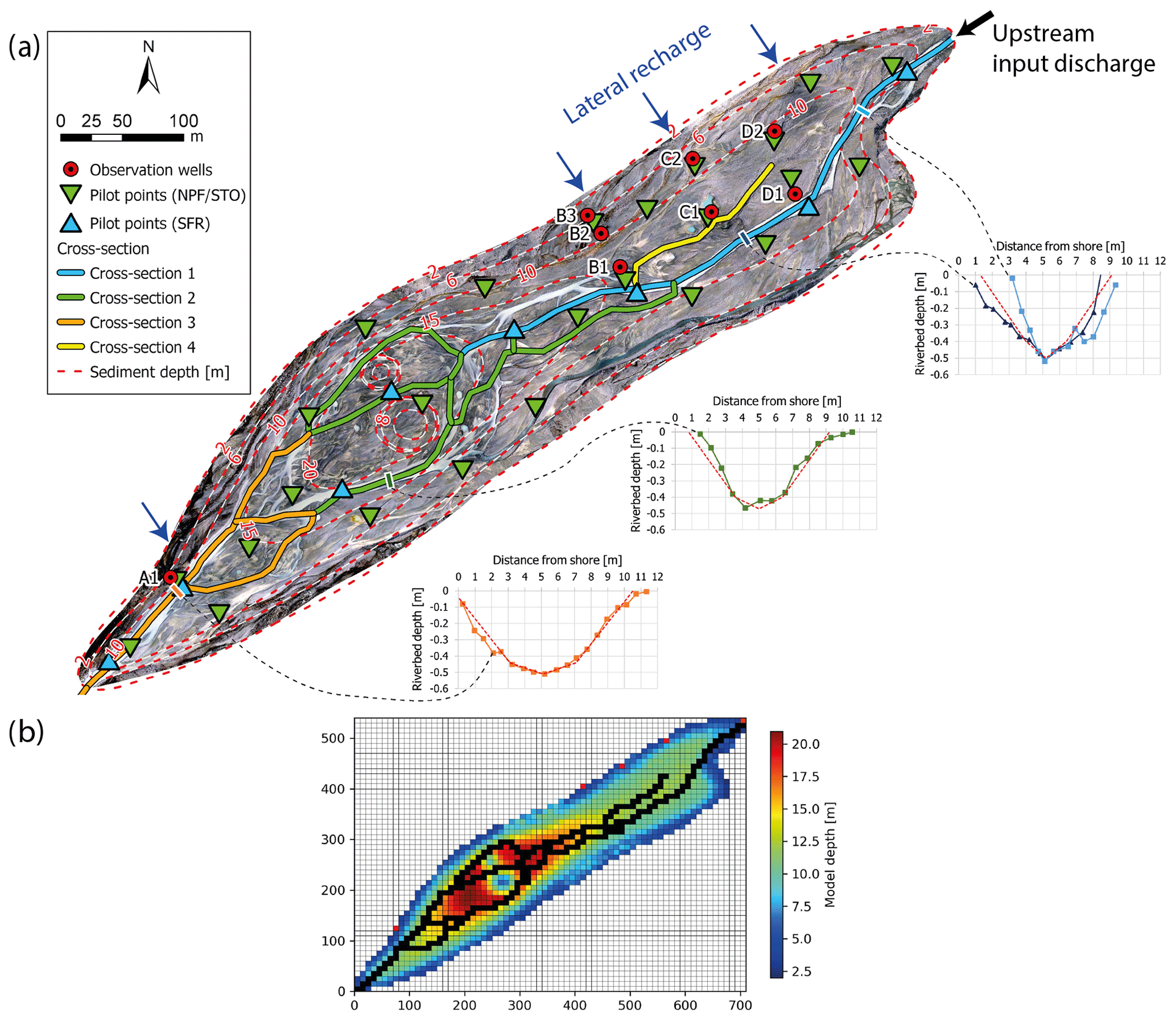
Figure 2 (a) Overview of outwash plain model parameters. Six pilot points are used for streamflow (SFR) and 15 for hydraulic conductivity (NPF) and storage (STO). Observation wells are used for history-matching. Sediment depth was drawn manually based on ERT profiles, and the two anomalies in the largest part of the floodplain are due to buried ice (see Sect. 4.1). The black arrow shows the upstream river discharge and the blue arrows indicate the locations of lateral surface recharge from the hillslope. River cross sections are separated into four classes: two bathymetric profiles are shown for cross section 1 (light or dark blue), one for cross section 2 (green) and one for cross section 3 (orange). The dashed red line in the graphs represents the corresponding simplified cross section used as model input. (b) Corresponding MODFLOW grid. The colour scale represents the maximal model depth. The stream network is shown in black and the red squares represent the location of recharge and input discharge.

The model uses the Newton–Raphson formulation, which allows for precise computation of unconfined saturated groundwater flow. Unsaturated flow above the water table is not considered, so that model cells in the unsaturated zone can only be either saturated or dry.

3.1.3 Streamflow routing (SFR)

The stream network was manually identified using the orthophoto from 18 August 2020 (Fig. 2). Only the main larger permanent channels were identified and were assumed not to change during the modelling period.

We use the SFR package from MODFLOW, which allows for an estimation of surface water–groundwater exchanges and an estimation of river stage and width based on Manning's equation, river discharge and riverbed cross section. For each river grid cell, the riverbed elevation was estimated using the calculated elevation from the surface DEM and an average depth for each stream segment based on a bathymetric survey performed on 18 August 2020, when a river cross section was measured with a differential GPS Trimble R10 and there was a spacing between points of about 0.5 m.

In the MODFLOW SFR package, river–groundwater exchanges are proportional to the difference between the aquifer head and stream stage. When the groundwater head drops below the bottom of the streambed sediments, the flux no longer depends on the aquifer head and is defined as the difference between the river stage and the bottom elevation of the streambed sediments (Langevin et al., 2017). This simplification may lead to underestimation of the fluxes for perched streams as no negative pressure in the dry cell below the stream is defined, as discussed in the work of Brunner et al. (2010).

A recent development in MODFLOW 6.3 is the definition of an irregular cross section which allows the river-wetted area to change with river stage and improves the estimation of the surface–groundwater fluxes. We defined a simplified cross section for each segment consisting of a trapezoidal section. Four different cross-sectional categories were defined (Fig. 2). The upstream river segments (category 1) have slightly steeper channel slopes and narrower bottom widths than the downstream parts (category 3); category 2 makes a transition between the upstream and downstream parts; category 4 represents a stream segment which was usually disconnected from the upstream river but where groundwater exfiltration maintained some baseflow in summer. This segment was defined with a rectangular cross section with a width of 2 m. MODFLOW first estimates discharge for each river cell and then calculates river stage and width based on the cross section, so that the wetted perimeter available for water exchanges varies with time. Manning's roughness coefficient was defined as a calibration parameter in the model.

3.1.4 Hillslope recharge

In addition to the river discharge defined for the streamflow, hillslope recharge was specified in the model. We specified four points of groundwater recharge on the side of the modelling domain (blue arrows in Fig. 2b), where a time-varying water input was applied in the first groundwater layer. Those recharge points represent the main observed ephemeral surface streams which drain the entire northern side of the hillslope above the outwash plain. We assume no diffuse recharge from the subsurface as such a flux could not be observed at the study site.

The amount of recharge was estimated by building an enhanced temperature index melt model (Gabbi et al., 2014), which computes snow accumulation and snowmelt as well as rain for the four selected hillslope subcatchments based on averaged hourly air temperature, incoming radiation and precipitation measured at the weather station. Precipitation was provided in summer by the weather station at the glacier tongue and winter precipitation from the closest available SwissMetNet station. The model was established at the catchment scale by defining model grid cells of 200 m, where mean elevation, slope and aspect were computed based on a 2 m resolution DEM from SwissTopo (2019). Snow redistribution on steep slopes was defined by limiting precipitation above a calibrated slope threshold. The incoming radiation was corrected for slope and aspect using a correction function defined by two calibration parameters. Model calibration was performed automatically using PEST HP (see Sect. 3.2) by minimizing the error in the calculated and measured snow water equivalent (SWE). SWE was estimated based on snow depth measurements performed manually at 5 locations on 26 June 2020 and 92 locations on 29 May 2021 on the whole glacier main lobe (from 2500 to 3000 m a.s.l.). Snow density was estimated by measuring the average density of the whole snowpack with a snow sampler in the centre of the glacier main lobe in 2020 and at two locations in 2021 on the same dates as snow depth. Additionally, in order to improve model performances (Hofmeister et al., 2022; Thornton et al., 2021), a second objective function was defined in PEST to minimize the error between the modelled and observed presence or absence of snow in each cell. Seasonal snow cover was based on daily 3 m resolution Planet images (Planet Team, 2017), where snow was identified using a K-means unsupervised learning algorithm from Google Earth Engine (ee.Clusterer.wekaKMeans, Arthur and Vassilvitskii, 2007). On average, one clear-sky day image was available every week in the summer. Both objective functions (SWE and snow cover) were first weighted equally, so that their total initial weighted sum of residuals is equal. Based on the initial calibration results, we then decided to increase the weight of the snow cover objective function to improve the representation of the snow cover fraction, which tended to decrease too quickly in the model during the late season. This iterative adjustment of the weighting resulted in total weights of 1 and 2.4 for the SWE and snow cover objective functions. Increasing the snow cover objective function contributed to better constraining the model parameters, especially for steep slopes where no SWE observations were available. This contributed to better matching of the evolution of the snow cover fraction over the melting season whilst maintaining a root mean square error of about 100 mm for the estimation of the SWE.

Finally, for the hillslope subcatchments, the same model was applied with the established parameter calibration, but we used 50 m elevation bands instead of grid cells as those subcatchments were too small for such grid cells. A simple routing to convey water from each elevation band to the subcatchment outlet was defined using a gamma distribution function, where the peak of the distribution matches the estimated transit time on the hillslope. The averaged transit time for a steep hillslope was estimated using a kinematic subsurface saturated flow equation (MacDonald et al., 2012), with a mean slope of 45^∘, an aquifer porosity of 0.3 and a hydraulic conductivity of 5 × 10⁻² m s⁻¹, which is typical for coarse talus slopes (Muir et al., 2011). The model codes and calibrated parameters are available in the Supplement.

Water input from the hanging glacier located on the southern hillslope (Fig. 1), either via hillslope recharge or directly via its tributary to the main network (near the end of the outwash plain), was neglected due to a lack of measurements in this part of the outwash plain.

Finally, after some preliminary modelling tests, we neglected the direct input of rainfall on the surface of the outwash plain as we could not observe any clear response from the groundwater from any rain events, and including this flux tended to lead to an overestimation of the groundwater heads.

The implications of the simplifications mentioned above are detailed in the Discussion section.

3.2 PEST HP

PEST HP is a model-independent algorithm for parameter estimation using inverse methods; model parameters are iteratively modified so as to minimize the variance of the error between the model outputs and the corresponding field observations (Doherty, 2015). PEST HP was used for calibration.

3.2.1 Calibration parameters and pilot points

The MODFLOW parameters selected for calibration are groundwater hydraulic conductivity (K_gw), groundwater specific yield (S_y), streambed hydraulic conductivity (K_rb) and Manning's roughness coefficient (n). Groundwater parameters govern the rate of groundwater flow in the subsurface and are typically used for model calibration against observations of the hydraulic head (Brunner et al., 2017). Riverbed hydraulic conductivity was also estimated as it was shown to have a strong impact on the rate of water exchanges between surface water and groundwater (Schilling et al., 2017). Manning's roughness coefficient was also calibrated as it is recognized as an effective parameter (Lane, 2014) designed to represent a set of processes not directly included, especially with the hydraulic formulation in MODFLOW used here.

Parameter estimation of the whole model domain was carried out by defining a subset of pilot points for calibration to which automatic kriging was applied. An exponential variogram with a nugget of 0, sill of 1 and range of 3 times the average distance between the pilot points was built using PEST groundwater utilities (MKPPSTAT and PPCOV_SVA). For K_gw and S_y, we place 25 pilot points separated by an approximately equivalent distance over the domain for all four groundwater layers. For the stream parameter K_rb, we use eight pilot points along the stream (Fig. 2).

3.2.2 Parameter regularization and initial values

To avoid unrealistically high spatial heterogeneity and over-fitting in the parameter estimation, we used Tikhonov preferred value regularization (Park et al., 2018), which adds a penalization term to the least-squares problem so as to dampen the influence of non-desired solutions. Preferred initial calibration parameter values are summarized in Table 1, and their initial values are assumed to be homogeneous in the model domain. For K_gw, the estimation was based on groundwater salt tracing and diffusive wave propagation was performed in the outwash plain in a previous work (Müller et al., 2022). There, we estimated saturated hydraulic conductivity values in the groundwater ranging from 85 to 660 m d⁻¹. We, therefore, defined here an initial value of 500 m d⁻¹ with a range between 10 and 2000 m d⁻¹ for K_gw. A similar value was also used in the work of Schilling et al. (2017) for a Quaternary alluvial aquifer. S_y was measured in the field with a mean porosity of 0.25 and was assumed to be homogeneous. Surface porosity on terraces with early vegetation was slightly higher, but this finer soil layer was shallow, so that the underlying sediments were similar to the rest of the outwash plain. Riverbed hydraulic conductivity could not be measured in the field directly, so that an initial value was estimated by manually running the model without automatic calibration, and it was set to 5 m d⁻¹. Finally, Manning's roughness coefficient was set to a value of 0.035 s m${}^{-\mathrm{1}/\mathrm{3}}$, adequate for natural unvegetated gravelly streams (Phillips and Tadayon, 2006) but with a calibration range of 0.01 to 0.05.

3.2.3 Objective function and model calibration

We use the time period from 15 August to 18 November 2020 for model calibration. Five different reference datasets were used to build a set of objective functions to calibrate the model with PEST: (i) daily averaged water head data from all eight wells; (ii) daily head differences; (iii) the daily time of maximal head; (iv) rate of daily head change; and (v) surface water–groundwater exchange fluxes along the main stream. We excluded the first 3 d of data from the calibration period in order to initialize the model. Such a short initialization period was used as the aquifer rapidly reached an equilibrium with the stream due to the highly conductive nature of the sediments in the outwash plain and the generally high groundwater levels in early summer.

The transformed datasets (ii) and (iii) were obtained from head measurements and contained additional information compared to the raw groundwater heads. It has indeed been shown that diel head fluctuations in fluvial aquifers are due to stream level variations that propagate as a diffusive wave into the aquifer (Magnusson et al., 2014). As suggested by Montalto et al. (2007), when the aquifer depth (b) is much larger than the water table variations, the magnitude of the diffusion depends on the mean aquifer transmissivity (T) in the whole aquifer and the aquifer porosity (S_y) in the zone where water fluctuations occur (see Eq. 1).

$$\begin{array}{}\text{(1)}& S_{\mathrm{y}}{\displaystyle \frac{\mathit{\delta }h}{\mathit{\delta }t}}=T{\displaystyle \frac{{\mathit{\delta }}^{\mathrm{2}}h}{\mathit{\delta }{x}^{\mathrm{2}}}}\end{array}$$

Since T=K_gw b, the amplitude and the delay of the diffuse wave are directly proportional to the integrated mean K_gw value of the aquifer between the river and the well through its entire depth. Therefore, using the groundwater fluctuations as an objective function forces the model calibration to better represent the average K_gw in the aquifer, i.e. at a depth lower than the groundwater wells.

The rates of daily head changes (dataset iv) were used to put more weight on the recession that occurs in autumn so that the rate of the aquifer drainage was well represented. Surface–groundwater exchange fluxes (resulting from surface water infiltration and groundwater exfiltration) were obtained from streamflow measurements along the main stream and corresponding differences between the upstream and downstream section ends (see Sect. 2.2 at the study site). Although the measurement was performed in 2021, we observed similar flow conditions (similar discharge at GS1 and groundwater heads) the year before, so that this observation of stream water–groundwater exchanges gave a first-order estimate of the fluxes during low flows and contributed to a better estimation of K_rb.

In total, we thus had five reference datasets for defining a calibration objective function corresponding to a non-linear weighted least-squares function. The calibration was then obtained with PEST by running the model 50 times until algorithm convergence. For all the other algorithmic parameters of the PEST algorithm, the suggested default values were used and are accessible in the Supplement.

Following the calibration procedure, we ran the model for the entire period for which we have data, i.e. from 27 June 2020 to 15 September 2021 (445 d), which yields us an additional 350 d to evaluate the model performance outside the calibration period.

3.3 Future of outwash plain storage and subglacial overdeepening mapping

Outwash plains are formed through successions of sediment aggradation and deposition which depend on sediment load, accommodation space, slope and discharge magnitude and intensity of variation (Miall, 1977; Maizels, 2002). In glacierized alpine catchments, valley bottoms are usually steep, so that suitable locations for the formation of outwash plains are restricted to areas where the bedrock topography is wide and flat. This mostly occurs where overdeepenings in the bedrock occur due to glacier erosion (Otto, 2019). If sediment supply fills such depressions, a new outwash plain may form. We therefore identified potential future outwash plains by locating bedrock overdeepenings below the current Otemma Glacier. The latest estimate of ice thickness distribution and corresponding bedrock topography for Switzerland was produced by Grab et al. (2021), where they used a mixed approach consisting of airborne ground-penetrating radar (GPR) profiles combined with glaciological modelling. Based on the DEM of bedrock topography with a resolution of 10 m, we automatically identify bedrock overdeepenings (ArcGIS Fill tool). We then manually defined a plane connecting the lower and upper edges of the identified overdeepenings, which would correspond to a theoretical outwash plain surface. We finally calculated the depth and volume of each future outwash plain by subtracting the elevation of the surface outwash plain DEM and the bedrock DEM.

Based on these results, we made the hypothesis of the emergence of additional outwash plains of similar volumes to the existing one and created a scenario where outwash plain aquifers would connect to each other; we also analysed the cascading effect on river discharge and aquifer storage. The aim here was to provide a qualitative and synthetic example of the processes as well as to approximate the order of magnitude of the impact of outwash plain groundwater storage and release on streamflow in the future rather than building a realistic and precise future scenario. We aim to only highlight the functioning of this specific landform and do not provide any projections for the entire catchment.

This aim was achieved by applying the developed MODFLOW model with the exact same dimensions sequentially to all the identified outwash plains, where river outflow from the upstream plain was used as streamflow input to the downstream plain. No future glaciohydrological model was developed to characterize the future inflow discharge. Instead, we simply used the measured discharge provided in this study for summer 2020 and then artificially created a linear (logarithmic-scale) discharge recession from 1 to 0 m³ s⁻¹ in 30 d in order to analyse the impact for a high-discharge or severe drought scenario. Lateral inflow from hillslopes was excluded here from the model in order to only analyse the impact of the floodplain on the cascading discharge.

4 Results

4.1 Bedrock topography

We present here the results of 3 ERT lines (of a total of 12 lines) collected in 2020, which cover different parts of the outwash plain (Fig. 3). The inversion results obtained are stable regardless of the chosen regularization parameter (lambda). Lambda values around 1 show coarser results, likely due to over-fitting; a mild regularization (lambda values of 10 to 50) leads to smoother images. The relative root mean square error (rRMSE) of most of the inversions is below 20 %, indicating low model misfit (Jordi et al., 2018).

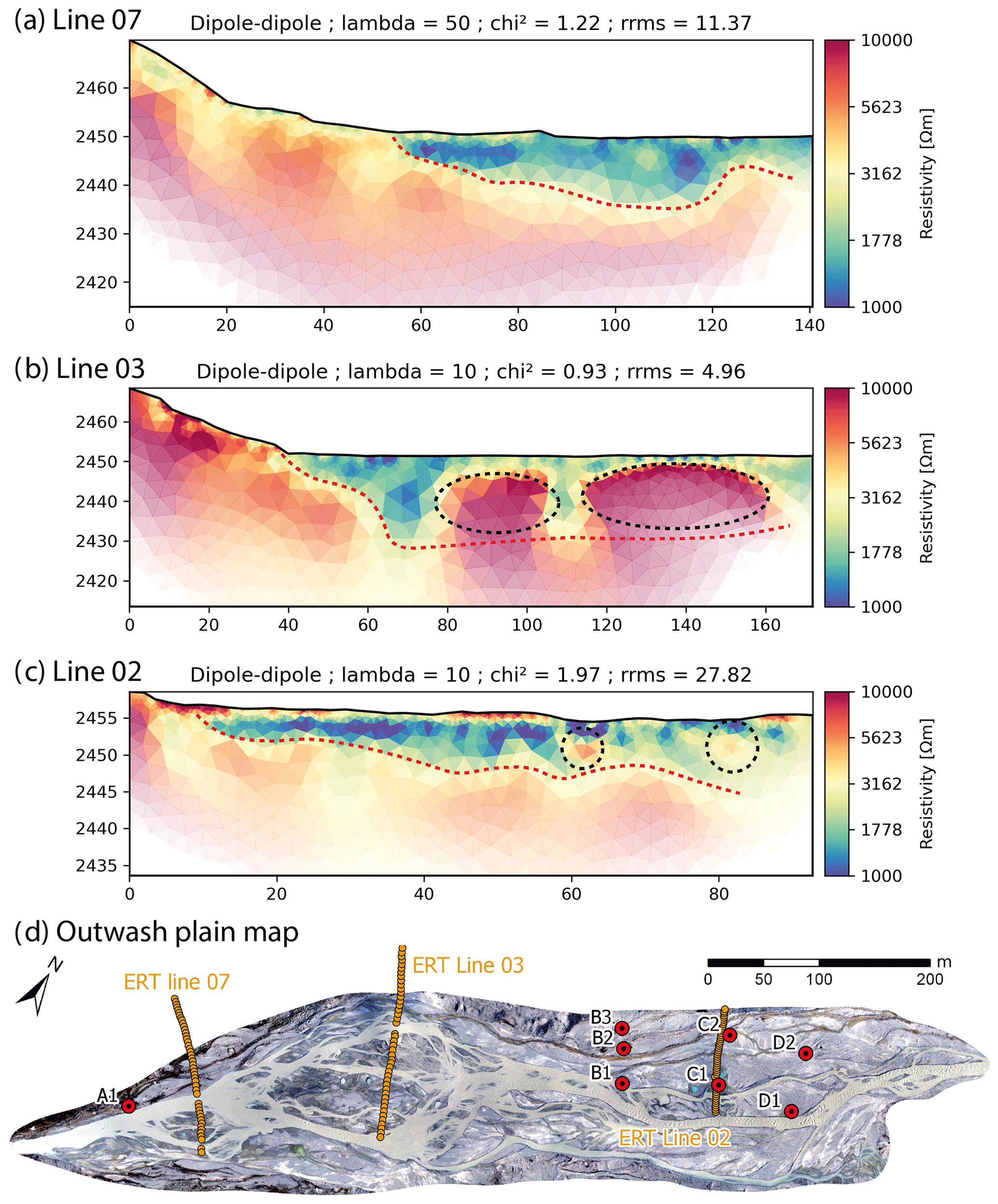
Figure 3 ERT profiles of (a) line 07 (electrode spacing of 3 m), (b) line 3 (electrode spacing of 4 m), (c) line 2 (electrode spacing of 2 m) and (d) corresponding locations of the ERT lines in the outwash plain. All the lines are oriented from the hillslope to the centre of the outwash plain. Red dashed lines correspond to the bedrock limit where the resistivity became larger than 2000 Ωm and black dotted circles highlight the location of buried dead ice with very high resistivity (>10 k Ωm). The regularization parameter (lambda) and the model performance are also indicated.

We compared the results from both the Wenner–Schlumberger and dipole–dipole schemes as well as intersecting ERT lines to assess the robustness of the bedrock depth estimation. The corresponding results agree well in most cases, in general with less than 10 % difference. Sediment depth increases smoothly from the hillslope edges of the outwash plain (with a depth of 2 to 5 m) towards its centre. The maximum sediment depth in the lower part of the outwash plain reaches 20 to 25 m (line 3 in Fig. 3) and 10 to 15 m in the upper part (line 2 in Fig. 3). Bedrock is also shallower at the upstream and downstream ends of the outwash plain, with sediment depths of only 2 to 5 m. The outwash plain therefore appears as a large bedrock overdeepening filled with sediments and showing a surface slope of 1 % downstream to 2 % upstream.

Some blocks of buried ice were also detected (Fig. 3). In line 2, two more resistant areas of 1 to 2 m in diameter can be identified in the middle of the sediment layer. These blocks were repeatedly measured for 3 years, with size and resistance slowly decreasing over the years. Since they are exactly located below kettle holes, which also became larger each year, these spots are attributed to slowly melting ice blocks, with a melting rate of less than 1 m in diameter per year. The ERT profile of line 3 also shows two more resistive (>10 000 Ωm) areas, which are much wider and deeper and reach widths of 20 and 40 m. Their elliptic shape and highly resistant nature indicate the presence of large zones of buried dead ice which fill a large part of the outwash plain. The presence of such large zones was only observed at this location, although daily imagery reveals kettle hole formation throughout the braidplain. Those two large buried ice blocks were directly included in the model as no-flow zones (Fig. 2a). Smaller blocks were neglected as they represent a negligible volume of the aquifer.

4.2 Surface water observations and electrical conductivity

River discharge at the glacier outlet was estimated continuously from July 2020 to September 2021 (Fig. 4a). The early melt season is characterized by high discharge but small diel variations, which can be explained by the incapacity of the distributed subglacial drainage system to rapidly evacuate large snowmelt water inputs. By August, diel fluctuations are larger as snow-line recession reduces buffering by the snowpack and the subglacial channel network has extended up most of the glacier (Lane and Nienow, 2019). Discharge starts to decrease in September, but a steeper recession starts in October. By early December, no more diel fluctuations are recognizable; discharge keeps decreasing slowly, with a minimum discharge of about 70 L s⁻¹ until March, when the first melt events occur.

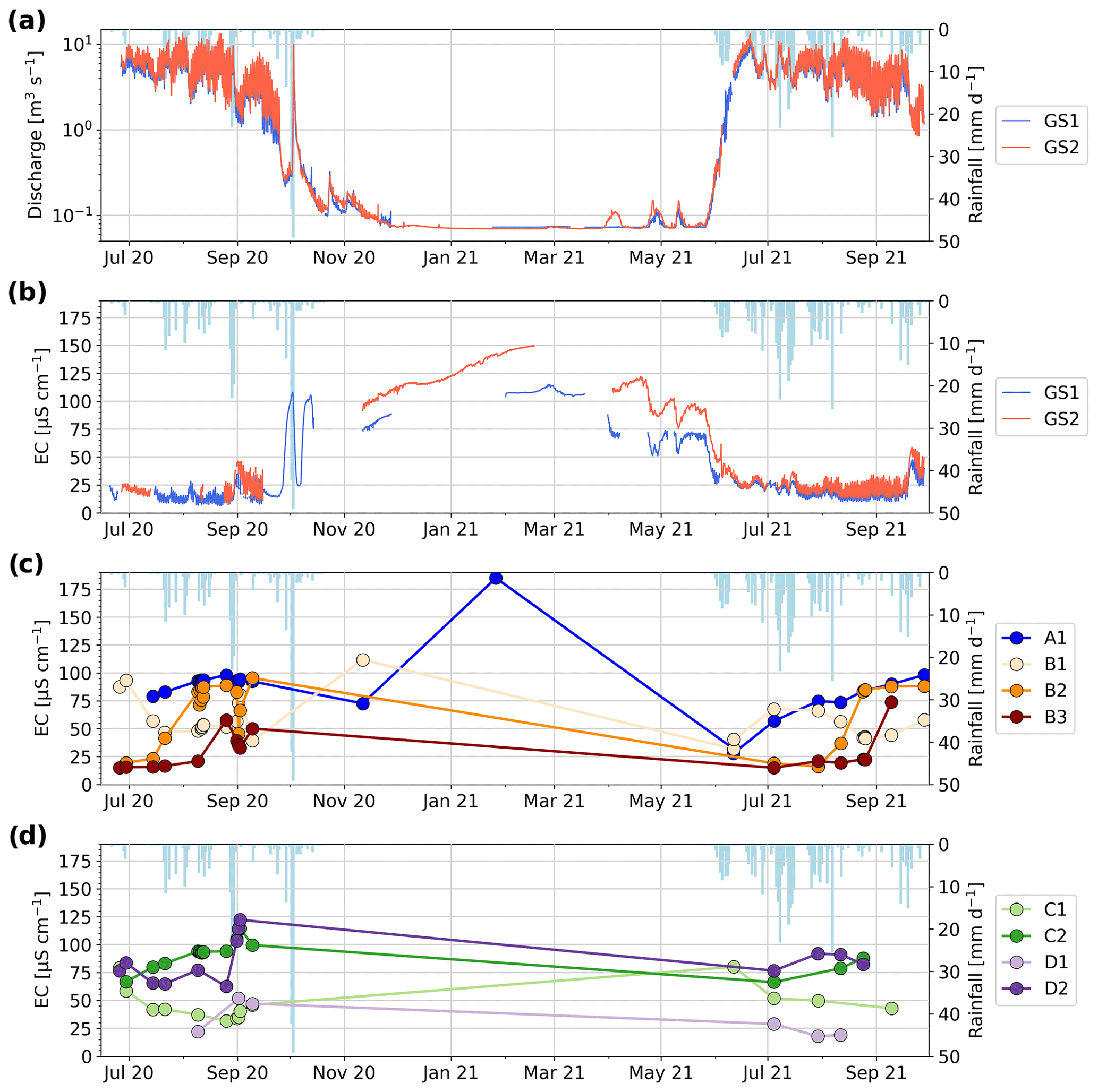
Figure 4 (a) Discharge measurements in the main stream at the glacier outlet (GS1) and at the end of the outwash plain (GS2); the y axis is in a logarithmic scale. (b) Electrical conductivity observations in the main stream and in observation wells (c) and (d). Measured daily rainfall amounts are also shown in light blue in all the plots.

Discharge at GS2 remains slightly larger than GS1, likely due to the ungauged glacial catchment, but the difference usually falls into the uncertainty margin of the discharge estimation. Water EC in the stream is inversely correlated with discharge (Pearson correlation of −0.84). In summer, EC varies between 10 and 25 µS cm⁻¹ at the glacier outlet (GS1) and is about 5 to 10 µS cm⁻¹ larger at the end of the outwash plain (GS2). During discharge recession, EC increases sharply, reaching values of 115 µS cm⁻¹ for GS1 and 160 µS cm⁻¹ for GS2 (Fig. 4b). This suggests that some stream water is provided to the outwash plain, also during the cold winter months, and is characterized by a steadily increasing EC. The origin of this stream water is not clear and may be due to some basal ice melt or a groundwater reservoir in the bedrock, as suggested in the work of Müller et al. (2022). The stream EC at the end of the outwash plain in winter shows higher values, which is likely due to groundwater contributions from the outwash plain area. This is further detailed in the Discussion section.

The wells close to the stream (D1, C1 and B1) tend to have low EC during summer, slightly larger than the stream EC, with a gradual increase in EC from the upstream well D1 to the more downstream well B1 (Fig. 4c, d). Well A1, also located near the stream but at the lower end of the outwash plain, has much higher EC values. The low EC in the upstream wells (D1, C1 and B1) indicates a strong influence from the nearby stream, and the EC increase from upstream to downstream suggests that groundwater tends to become older with greater distance from the upstream part of the outwash plain. In particular, the high EC values of well A1 indicate that here we find the longest groundwater flow paths, with no direct exchanges with the nearby stream.

The wells closer to the hillslopes (D2, C2 and B3) show higher EC than the wells located at the same transect near the stream. Here, high EC may be due to either (1) long groundwater flow paths from the stream reach or (2) lateral hillslope recharge from a source characterized by higher EC than the stream.

Wells B2 and B3 show very low EC values in the early melt season (Fig. 4c), which is due to a connection to an ephemeral hillslope tributary characterized by low EC values (10 to 20 µS cm⁻¹) related to snowmelt input via surface runoff. This recharge seems to be only dominant during the early snowmelt at this specific location.

In summary, EC in wells is highly spatially and temporally variable due to a combination of different water sources with varying EC compositions and varying degrees of connectivity with the stream. In general, EC in the wells seem to be correlated with their distance to the upstream part of the outwash plain, with well D1 showing an EC very similar to the stream EC, suggesting a strong river infiltration from the upstream stream reaches. The contribution from lateral hillslope groundwater will be further assessed based on the modelling results.

4.3 MODFLOW model calibration

The average calibration results obtained with PEST HP for K_rb, K_gw, S_y and n are shown in Fig. 5; the corresponding initial parameter values and calibration ranges are summarized in Table 1. The K_gw of each layer shows some spatial variability, with zones of higher conductivity in the upper layers (400 to 1200 m d⁻¹) leading to somewhat larger average values for the top layer (Fig. 5a). Aquifer porosity (S_y) shows local variability in the top two layers, while the initial values were retained for the third and last layers (Fig. 5b). The riverbed hydraulic conductivity (K_rb) was estimated as having values between 3.5 and 15 m d⁻¹, with a tendency to increase in the lower half of the braidplain (Fig. 5c). Although Manning's roughness coefficient was on average close to the initial value of 0.035 s m${}^{-\mathrm{1}/\mathrm{3}}$, it varied systematically and spatially between higher (up to 0.05) and lower (0.02) values. The modelled groundwater levels matched well with the observations, and the timing of the daily peaks had an average RMSE of 1.56 h (Fig. 6). The median relative errors of diel head amplitudes and diel head changes for each well (absolute residuals divided by the observed value) are shown in Fig. 6; they show satisfying results, with diel head amplitude errors smaller than 20 % and modelled head changes showing similar trends to the measured ones.

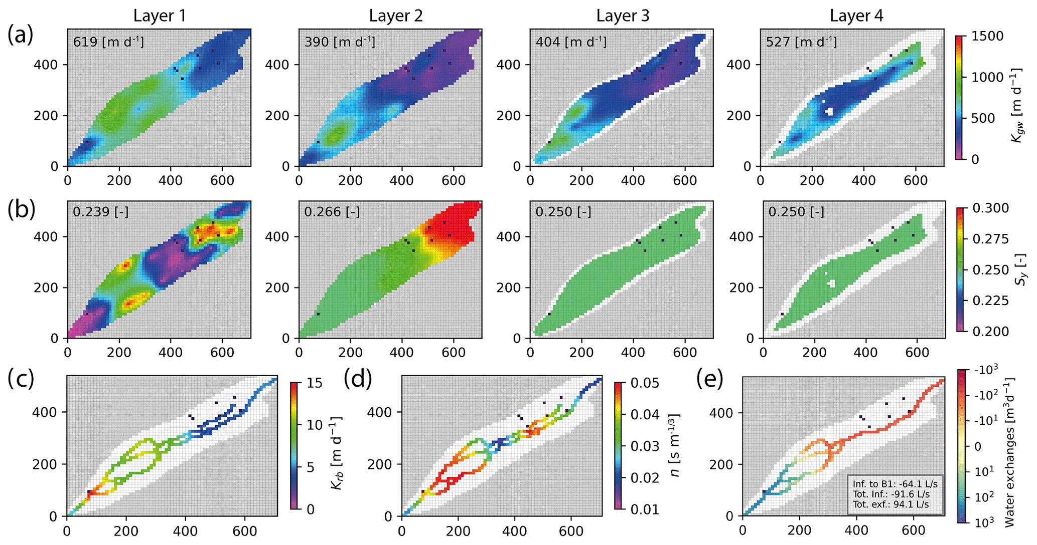
Figure 5 Results of parameter estimation using PEST HP. (a) Groundwater hydraulic conductivity (K_gw) and (b) aquifer porosity (S_y) for the four groundwater layers. The parameter numbers correspond to the average value in the whole domain. (c) Parameter estimation for the riverbed hydraulic conductivity (K_rb). (d) Parameter estimation for Manning's roughness coefficient (n). (e) Corresponding modelled surface–groundwater exchanges on 17 November, with the text indicating modelled infiltration (until well B1 and in total) and total exfiltration. Black dots correspond to the locations of the observation wells. The grey-shaded areas are outside of the model domain, and white indicates the area where the layer does not exist. The X–Y values correspond to the model grid coordinates in metres.

Observed versus modelled groundwater heads

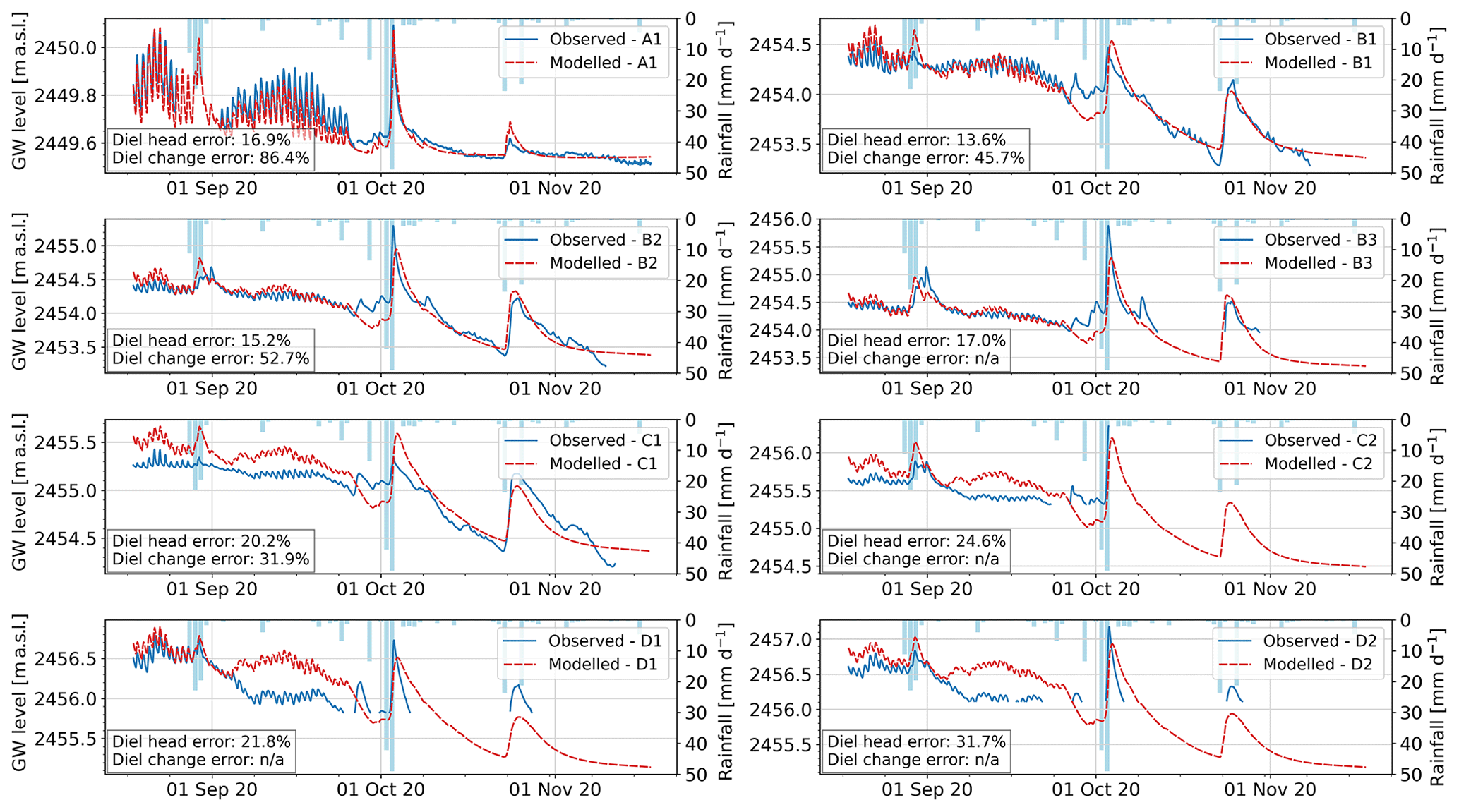
Figure 6 Observed (blue) versus modelled (dashed-red) groundwater heads for each well (A1 to D2). Mean absolute relative errors for the diel head amplitudes and diel head changes are also shown in the lower-left box. No error is estimated (n/a) for the rate of change of wells where the autumn recession could not be measured.

Groundwater infiltration on 17 November in the upstream part of the catchment (until well B1) is somewhat overestimated, with 64.1 L s⁻¹ compared to the observed 30 L s⁻¹; the net streamflow difference between upstream and downstream discharge is underestimated, with a net water gain for the stream of 2.5 L s⁻¹ compared to an observed water gain of 8.3 L s⁻¹ (Fig. 5d).

4.4 MODFLOW model validation

For the additional 12 months simulated for model evaluation, the model performance for diel head amplitudes and for the timing of diel peaks is similar to the calibration period. The daily averaged heads for three observation wells are shown for illustration purposes in Fig. 7. In addition, we also show the results of a model run where all the tributaries are removed so that upstream discharge is the sole water input.

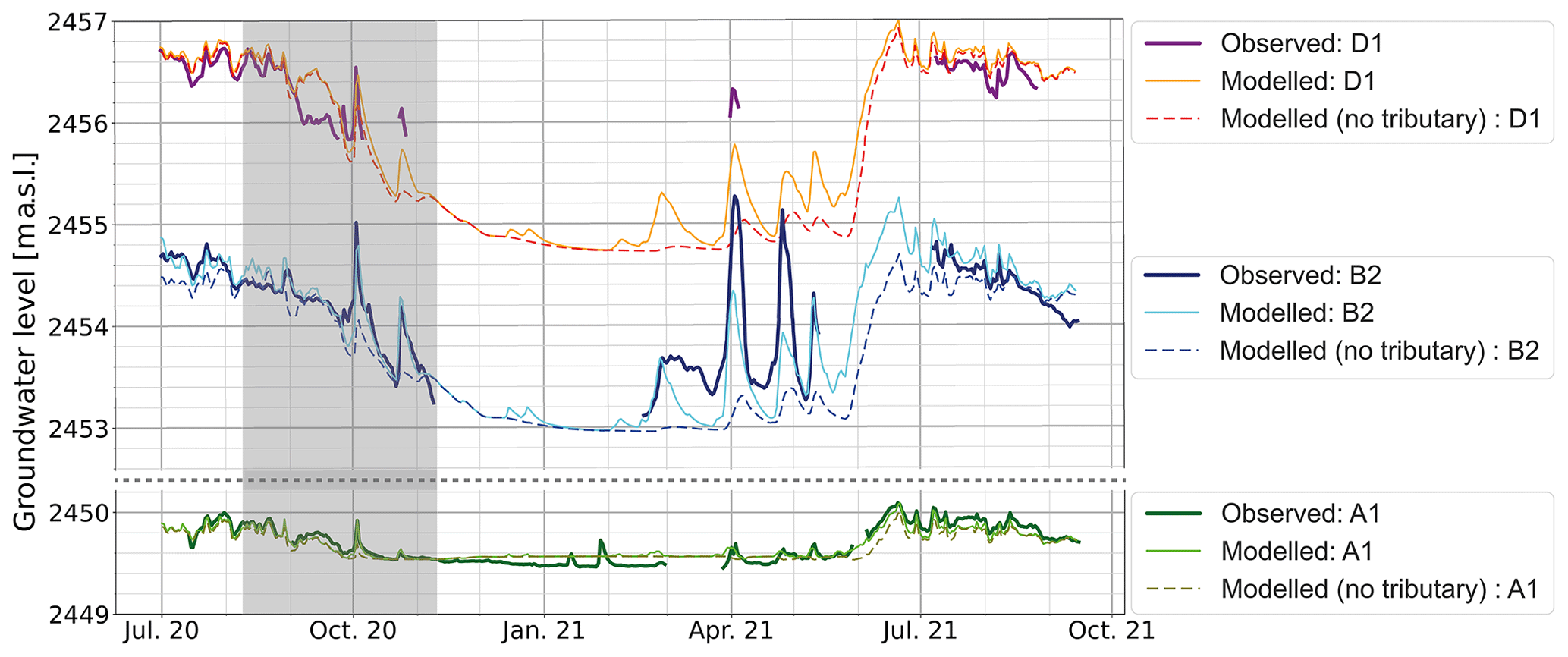
Figure 7 Observed versus modelled groundwater levels for three selected wells during a 14-month period. The dashed lines represent model results when all the hillslope water input is set to zero during the entire simulation. The shaded area represents the calibration period. Note that the y axis is cropped between wells A1 and B2, but the scale is the same.

Over both summers, groundwater levels appear well simulated under both high- and low-flow conditions. For well D1, there is a slightly larger offset between observed and modelled heads in 2021, and the decrease in head occurring in late August to September 2020 and 2021 does not seem to be well modelled, although the head catches up again in October 2020. This latter phenomenon is likely due to some changes in the structure of the river channel that were not incorporated into the model. For both summers, wells B2 and A1 appear to match the observations closely.

During winter, the slight groundwater recession in well A1 is not fully well represented. This may be due to the lower bedrock edge of the outwash plain which may be somewhat deeper than modelled, constraining groundwater exfiltration in this lower part. For well B2, the simulated groundwater level in mid-February 2021 matches the observation, supporting the good performance of the model in simulating groundwater drainage during low winter flow. The first initial recharge event in late February is also well modelled, but the next two short peaks (April and May 2021) are underestimated. This is likely due to an underestimation of the lateral hillslope recharge or direct snowpack melt on the outwash plain, which was not included in the modelling framework.

4.5 Groundwater storage and surface water–groundwater exchanges

Infiltration of stream water to groundwater occurs preferentially in the upper half of the floodplain and exfiltration of groundwater to the stream occurs in the lower half (Fig. 5d) of the plain. Summer infiltration is proportional to discharge, with a maximum infiltration rate of about 400 L s⁻¹ and a minimum rate of 60 L s⁻¹. Some hysteresis is visible: for similar discharge, more infiltration occurs in the late morning (10:00 to 14:00 UTC +2), when groundwater levels are low, than in the night, when groundwater levels are high (Fig. 8a). In summer, exfiltration of groundwater is also correlated with stream water infiltration: the lowest exfiltration rates occur in periods with increasing infiltration rates and discharge, and the highest exfiltration rates occur during periods of decreasing infiltration and when groundwater levels are high (Fig. 8c).

During discharge recession in winter, discharge decreases sharply and infiltration is reduced proportionally. The decrease in infiltration is mainly due to a change in the wetted perimeter of the stream reach, limiting the surface area for water exchanges. This change is more marked for the upstream stream reaches, whose channel banks are steeper than the downstream sections (Fig. 2).

When discharge decreases below 85 L s⁻¹, most of the stream water infiltrates the upper half of the outwash plain (Fig. 8b), so that the main stream retains little surface water in the central part of the outwash plain. However, at low discharge, exfiltration in the lower half is slightly higher than infiltration (Fig. 8d), leading to more stream discharge at the end of the outwash plain than upstream.

In summer, it appears therefore that the outwash plain is only capable of infiltrating small amounts of water from the stream; infiltration happens preferentially in the morning. The aquifer exfiltrates a similar amount of water with a peak during the night, so that the average daily groundwater level remains relatively constant. In winter, most of the upstream river discharge infiltrates from the stream to the aquifer, but a slightly larger amount exfiltrates from the aquifer, leading to a gradual decline in the aquifer level. The aquifer therefore sustains a higher discharge at the downstream end of the outwash plain than at the upstream end. The observed slow rate of aquifer recession throughout the winter is due to a small but constant upstream water input, i.e. upstream discharge recession.

The rate of decline is illustrated in Fig. 9. In summer, groundwater is maintained close to the surface in the entire plain, with distances of about 0.5 to 1 m from the surface in the upstream part and 0.1 to 0.5 m in the downstream part. The total water storage in the outwash plain in summer equals 3.0 × 10⁵ m³, which is equivalent to 10.0 mm with respect to the entire catchment area (30.4 km²). It appears clearly in Fig. 9 that a large part of the aquifer volume is located below the lowest edge of the bedrock, so that this volume cannot empty. The water amount which can exfiltrate from the groundwater to maintain river discharge is hereafter defined as the dynamic storage (Staudinger et al., 2017) and corresponds to 6.7 mm (relative to the catchment area) or 67 % of the maximum total storage. In winter, the groundwater level gradually declines from the upstream end of the outwash plain but remains close to the surface in the lower part, where groundwater flow is constrained by bedrock and forced to exfiltrate. At the time of lowest discharge (1 February 2021), the total dynamic storage amounts to 5.4 mm, so the aquifer has lost 1.2 mm during the recession period.

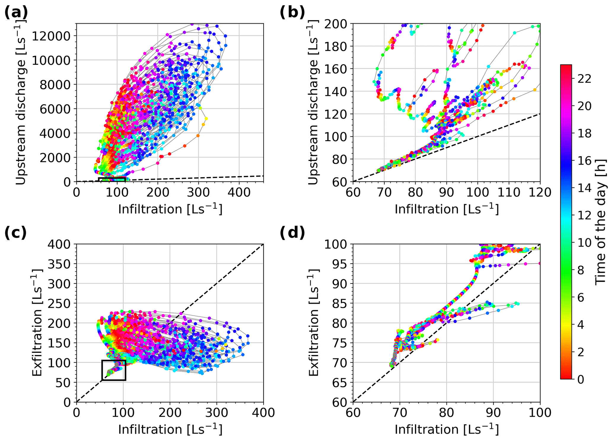
Figure 8 Surface water–groundwater exchanges. (a) Relationship between river reach infiltration and incoming upstream river discharge. (c) Relationship between river reach infiltration and groundwater exfiltration into the stream. The black rectangles indicate the zone of the zoom-in windows of the graph on the right: (b) and (d). The colour scale corresponds to the hour of the day for each point. The straight dashed lines show the line of equal values.

Modelled groundwater levels for different dates along a vertical cross section of the outwash plain

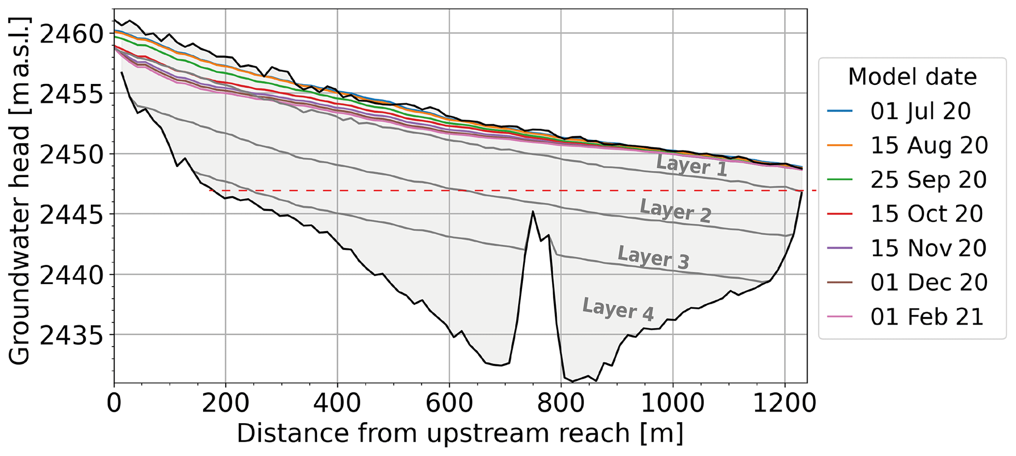
Figure 9 Modelled groundwater levels at different time steps (dates) along a vertical cross section of the outwash plain, from the top-right corner (upstream reach) to the bottom-left corner (downstream reach) of the model domain. The grey area represents the whole aquifer with the four groundwater layers, and the black lines represent the bedrock and surface limit of the model. The steep jump between distances of 700 to 800 m represents the location of the buried ice from ERT (Fig. 3), which is defined as bedrock in the model. The dashed red line indicates the lower limit of the dynamic storage, below which groundwater heads cannot drop.

4.6 Future hydrological role of the outwash plains

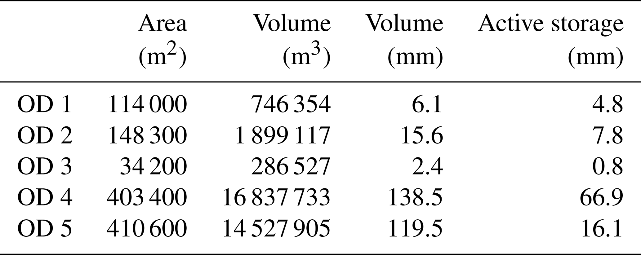
We identified five bedrock overdeepenings below the Otemma Glacier main lobe (Fig. 10) and quantified their dynamic storage by calculating the volume included between the sloping aquifer and the horizontal line at the lower edge of the overdeepening and using a porosity of 0.25 (Table 2). The lowest two overdeepenings show similar areas and volumes to the current outwash plain. The third one is limited to a smaller volume of sediments with a storage potential of about 10 mm. The two upper ones are characterized by much deeper depths and larger volumes.

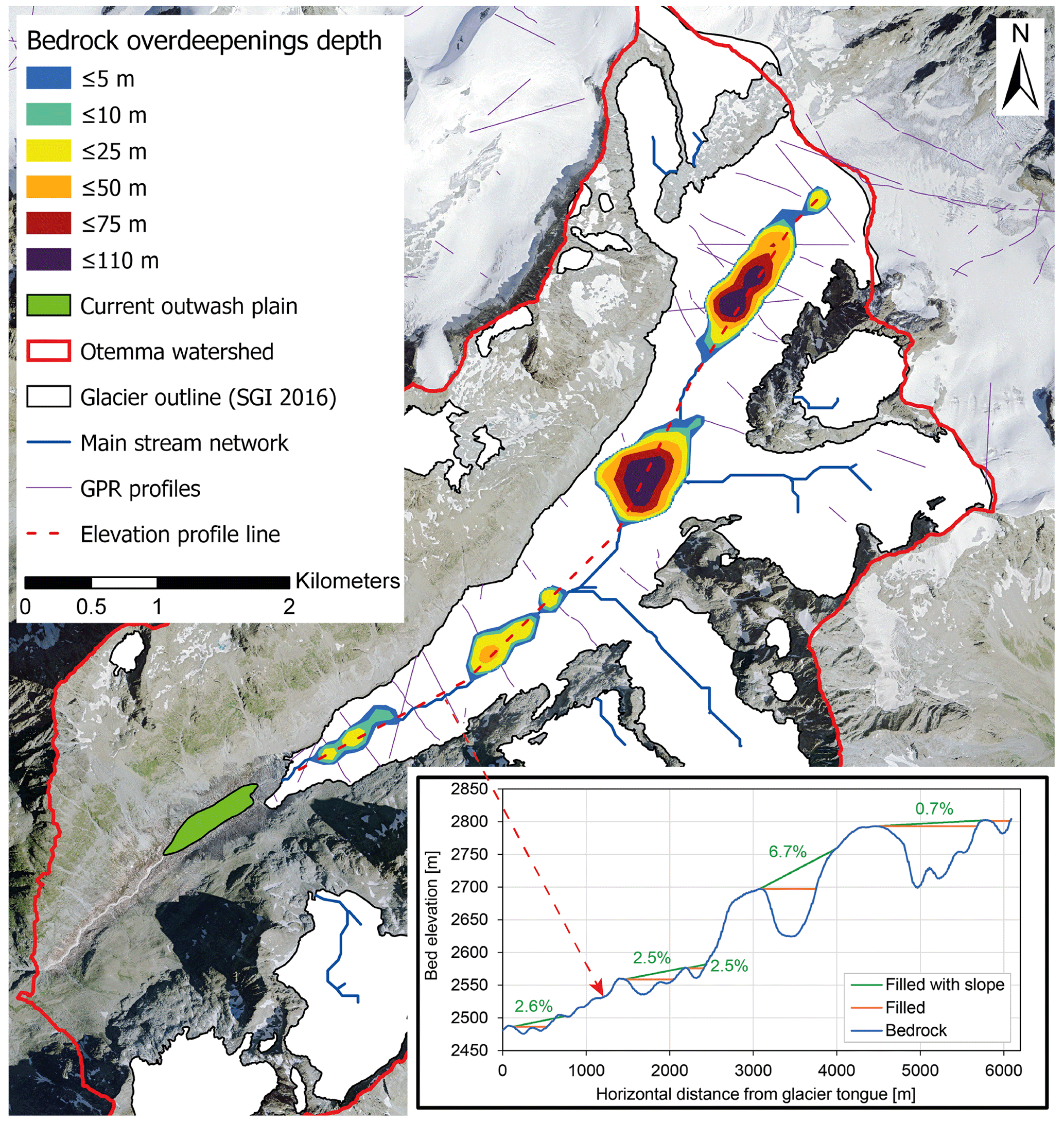
Figure 10 Mapping of the Otemma Glacier overdeepening estimate based on the bedrock topography provided by Grab et al. (2021) with depth below a gently sloping plane connecting the lower and upper edges of the overdeepening. An elevation profile of the bedrock along the glacier main lobe is also highlighted with the dashed red line and the profile is illustrated in the bottom-right graph in blue. In the graph, the green line shows the slope of the planes used to fill the bedrock overdeepenings, while the orange line represents the horizontal limit from the lower edge of the overdeepening. Airborne GPR profiles from the work of Grab et al. (2021) from which topography is estimated are also shown in violet. The main stream network was calculated using flow accumulation (ArcGIS pro v2.3) based on the bedrock topography map. The current outwash plain is shown in green outside the glacier area (white area). The background image was provided by SwissTopo (2020).

Based on the hypothesis of the future emergence of two new outwash plains, we analysed the cascading effects of a chain of three outwash plain aquifers. The results depicted in Fig. 11a) show that, for high flows, a slight reduction of the peak discharge occurs. In the first outwash plain, river infiltration amounts to about 350 L s⁻¹ of stream water when peak discharge reaches 13 m³ s⁻¹; the aquifer simultaneously releases about 180 L s⁻¹, leading to a decrease in the total discharge of about 170 L s⁻¹. At the end of the third plain, the total peak flow reduction due to infiltration is about 400 L s⁻¹. The peak is also slightly delayed and attenuated due to flood routing along the braided river system, leading to a total decrease of about 600 L s⁻¹, i.e. slightly less than 5 % of the upstream water input.

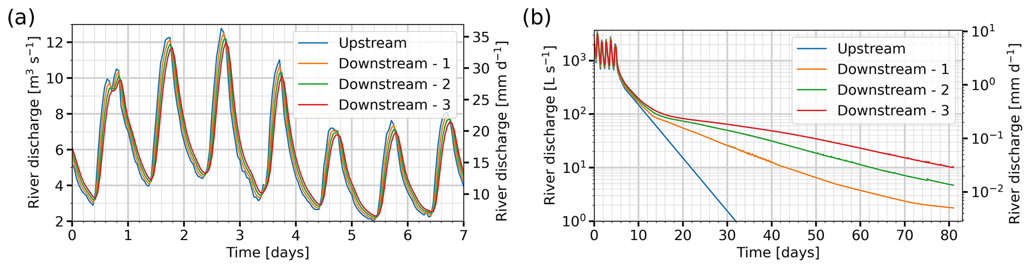
Figure 11 Simulated impact on stream discharge for a hypothetical chain of three outwash plains. (a) Discharge estimation for high discharge and (b) baseflow estimation, resulting from a theoretical input discharge (blue) and modelled outflow discharge from a first outwash plain (orange) to a second plain (green) and a third one (red). In panel (b), the y axis is in the logarithmic scale. The secondary y axis indicates the corresponding discharge in millimetres per day at the catchment scale (30.4 km²).

Table 2 Estimated volumes of the five glacier overdeepenings (ODs) from lowest (no. 1) to highest (no. 5) along the glacier main lobe of the Otemma Glacier. The volume in cubic metres represents the total “empty” space, and the volume in millimetres corresponds to the total potential groundwater storage relative to the catchment scale (30.4 km²) assuming a porosity of 0.25. The active storage represents the groundwater storage above the horizontal line (Fig. 10).

For the drought scenario (Fig. 11b), after the first outwash plain, higher downstream river discharge is only maintained when the input discharge decreases below 180 L s⁻¹ (or about 0.5 mm d⁻¹) on day 10. The rate of discharge recession is fast, with the discharge decreasing by half in about 4 d and decreasing by 10 times in about 25 d, leading to an emptying of 85 % of the total dynamic storage. In the case where three outwash plains are interconnected, river discharge remains similar to that with only one outwash plain before day 10. When the discharge decreases below 180 L s⁻¹, the discharge recession rate becomes slower, leading to discharge decreasing by half in 8 d and by 10 times in 54 d. Thus, slightly more discharge can be expected during droughts with a chain of outwash plains, with a discharge recession rate about twice as slow.

5 Discussion

We first discuss below the limitations related to the simplifications and assumptions used here to set up the MODFLOW model. We then review the insights gained into the hydrogeological behaviour of the outwash plain in Otemma and compare field observations with results from the numerical model. Finally, we discuss what future hydrological changes may be expected in the Otemma catchment when considering potential future outwash plains and in particular in the case of future droughts or high-flow events. We conclude with some more general implications from both an ecological perspective and a more methodological perspective.

5.1 MODFLOW model limitations

5.1.1 Model structure

We used ERT to constrain the depth to the bedrock at specific locations. Although inversion results lead to a clear transition between water-filled sediments and bedrock, an error of a few metres cannot be excluded. The bedrock depth was interpolated between the ERT profiles, which leads to a larger uncertainty in areas distant from those lines. We only defined four aquifer layers with vertically constant parameters, while lenses of silt and sand are distributed at much smaller scales, as observed in sediment facies (Maizels, 2002). The spatial parameter interpolation between the pilot points in each layer also does not allow us to form specific flow paths, as we used no particular training image. That is, we did not impose any specific patterns (Mariethoz et al., 2010; Orsi et al., 2016). This leads to a clear oversimplification of the heterogeneity of such a fluvial aquifer. As a result, our parameter estimation does not allow for the formation of preferential flow paths, which may increase drainage and groundwater levels in specific parts of the outwash plain (Cozzetto et al., 2013). These limitations are at least partly mitigated by performing a calibration designed to fit not only groundwater levels but also a set of aquifer behaviours. As such, even though our groundwater wells are shallow (about 2 m deep), K_gw could be better constrained with depth by matching the amplitude of diel groundwater variations, which leads to a reliable estimate of the depth-averaged value of K_gw (see Sect. 3.2.3). Even if preferential flow paths exist, the rate of groundwater drainage is constrained in the calibration by the rate of groundwater recession in autumn and the measured rate of groundwater exfiltration in the lower part.

5.1.2 Superficial vadose zone and input fluxes

In this study, we neglected the vadose zone. The fine sediment texture was composed of more than 90 % sand and usually less than 1 to 2 % clay. This leads to a soil texture dominated by large pores where the capillary effect is limited. This was tested using HYDRUS-1D (Šimůnek and van Genuchten, 2008), which solves Richard's equation and allows accurate modelling of the interface between a saturated zone and an unsaturated zone. It shows that the unsaturated water content above the water table drops rapidly to values close to 0.05 in the first 50 cm of unsaturated sediments. This is due to the dominance of large pores and relatively coarse sediment. Consequently, the unsaturated water content decreases rapidly when the water table drops, and so does the unsaturated hydraulic conductivity, leading to a very dry soil surface, where actual evapotranspiration is strongly limited. Additionally, residual water content in the vadose zone should have a limited effect on diel groundwater fluctuations.

We also neglected the direct recharge from precipitation falling on the surface of the sediments in the outwash plain. This choice is reasonable since this water input is small compared to stream water infiltration. Indeed, on average for each day, average stream water infiltration amounts to about 100 to 150 L s⁻¹ (see Fig. 8) or 10⁴ m³ d⁻¹, which is similar to an equivalent precipitation amount of 110 mm over the whole outwash plain. This indicates that the direct rainwater input is only significant during days of heavy rain but does not represent a large part of the seasonal recharge as the total liquid precipitation represented only about 250 mm in 2020. Precipitation seemed indeed to only impact groundwater levels for rain events larger than 10 mm d⁻¹ (Fig. 6), but the rapid recession of the groundwater head seems to indicate that transmission of the rainwater through the vadose zone is fast and that water retention in the unsaturated sediments is limited after the day of the event. Moreover, in our model, we only accounted for lateral recharge during such rain events, but model results show a similar groundwater response to the observed one, suggesting that the additional input of rainwater on the surface did not influence the groundwater levels much (Fig. 6). The reason for this lack of response to the rain input on the surface is likely due to the effect of the dry unsaturated zone, which partly retains the rainwater infiltration in the unsaturated zone and/or preferential flow paths in the sediments that limit diffuse surface recharge and limit surface water infiltration to specific locations within the outwash plain or rapidly drain this water into the braided stream. Since the groundwater head did not respond to most rain inputs, we believe that neglecting the unsaturated zone, together with the direct input of water from precipitation falling on the sediments, allows for an adequate simplification of the model which aims at modelling the seasonal groundwater behaviour of such a system and not specific processes in the vadose zone.

Finally, we also neglected the contribution from the small hanging glacier on the upper southern side of the outwash plain, although it clearly provides additional recharge. This choice is due to the lack of groundwater and discharge observations in this area and thus a lack of means to quantify the input discharge. As discussed before, we have shown that the main behaviour of the aquifer can be explained by the incoming upstream discharge and that any additional lateral water input likely only affects the local groundwater levels but does not modify the seasonal-scale dynamics.

5.1.3 Stream channels and surface–subsurface processes

Geomorphological changes in the outwash plain were also not taken into account. Strong cycles of sediment deposition and aggradation modify on daily and seasonal timescales the shape of the riverbed and the number of stream branches. Indeed, on a daily basis, some transient channels will appear during high discharge and disappear during low flow, which influences the total wetted area and thus modifies the rate of stream infiltration and groundwater exfiltration. This phenomenon appears especially important in the lower half of the braidplain, as is clearly visible in the orthoimage (Fig. 2), where we only defined three permanent channels. Using Manning's equation and a v-shaped cross section, we estimated that a hypothetical addition of 10 ephemeral branches would lead to an increase of 200 % in the total wetted area and a decrease of 20 % in the river stage. Such changes are not negligible but can at least be partially compensated for by the calibration procedure by adapting the riverbed hydraulic conductivity (K_rb) and Manning's coefficient (n). The calibration procedure seems indeed to lead to such compensation, as both K_rb and n were estimated to be larger in the lower half of the plain (Fig. 5c, d), which allows for larger exchange rates between river water and groundwater. Higher n values in the lower part are also expected from a geomorphological perspective due to a more irregular, larger and flatter channel cross section (Phillips and Tadayon, 2006). n also appears lower in straighter parts of the river network and higher in zones of flow convergence where more flow turbulence may increase flow resistance and decrease velocity. The local variations in the estimation of n may however also arise more artificially from the calibration procedure, which attempts to match the diel amplitude and the timing of the groundwater fluctuations. The higher estimated n value near well B1 is likely due to increased diel stream variations, which have a direct impact on the nearby well and thus locally compensate for some uncertainties in the simplified river morphology.

Some limitations regarding the coupling between surface and subsurface flow in MODFLOW have been discussed previously (Brunner et al., 2010). In particular, the absence of negative pressure in cells below the streambed when the stream becomes perched in winter may lead to some uncertainties in winter. Nonetheless, the estimated K_rb for the upstream reaches is between 3 and 15 m d⁻¹, similar to another study of a Quaternary glaciofluvial aquifer where the retained K_rb value was 2.4 m d⁻¹ (Schilling et al., 2017). Since we mostly analyse the model results in terms of processes during the period of calibration when field observations are available, we believe that such limitations are at least partially relaxed and do not significantly impact the results. In the lower half of the plain, however, the estimated K_rb values were larger, which is likely due to the calibration procedure attempting to balance the lack of some secondary channels and somewhat artificially increasing the exfiltration rate.

Despite the overall good performance, there are some notable differences between observations and modelled groundwater heads. For instance, during September and October 2020, wells D1 and D2 have a modelled water head about 0.5 m higher than measured (Fig. 6). This is due to a change in the stream reach at this location, which moved further away from the wells and eroded vertically, leading to a decrease in the head. This illustrates that our model fails to locally reproduce the exact depth of the groundwater, and this issue is likely more important where no groundwater observations are available.

Our estimation of groundwater–surface water exchanges relies on streamflow observations at only two locations on a single day, which might in particular lead to uncertain exchange fluxes during low flows and may reduce the capacity of our model to accurately reproduce exchanges during very dry periods.

5.1.4 Modelling framework

In contrast to many other studies, our goal in this work was to focus on the hydrological functioning of a subpart of an alpine glacier forefield (the outwash plain) rather than to provide predictions for the entire catchment. We attempted to include all major processes that influence the seasonal groundwater dynamics of this landform by building a complex groundwater model linked to a simpler surface hydrological model to simulate lateral recharge. Nevertheless, this approach leads to the series of assumptions discussed previously. Alternatively, recent research in alpine catchments (Thornton et al., 2022) has attempted to provide fully integrated approaches such as Parflow (Maxwell and Miller, 2005) or HydroGeoSphere (Kolditz et al., 2012), which could relax some of the uncertainties discussed in this work. However, such models typically require heavy data acquisition, limiting their applicability in alpine environments (Ala-aho et al., 2017). In this work, we believe that this simpler model combined with an adequate multi-objective calibration procedure provides more control and understanding of the key processes which occur in the outwash plain aquifer specifically. Indeed, the calibration allowed the model to reproduce the aquifer behaviour reliably and, in particular, the aquifer levels throughout the year, the aquifer drainage rates and the rates of infiltration and exfiltration. In particular, even with a static definition of the geomorphology, the long model runs over 14 months (Fig. 7) show that the average level of all the groundwater wells could be satisfyingly reproduced.

5.2 Outwash plain groundwater dynamics

The outwash plain appears to recharge rapidly in the early melt season from the hillslopes and from the main stream. Hillslope recharge provides significant recharge, especially in the early melt period (March to June in Fig. 7), but is rapidly drained when less melt occurs. Groundwater levels increase synchronously with stream discharge in early June and maintain a high level, even when hillslope recharge is largely reduced in later summer. Thus, although hillslope tributaries maintain locally higher groundwater heads (up to about 1 m for well B2 in Fig. 7), it is the moderate but constant river infiltration from the stream which maintains groundwater levels close to the sediment surface during the snow-free season (Fig. 7) and which drives the seasonal groundwater dynamics.

This behaviour was validated by EC observations made in the groundwater wells. Wells close to the hillslope (B3, C2 and D2) tend to show a gradual increase in EC from June to September (Fig. 4), which correlates with a gradual decline in hillslope discharge and a lowering of groundwater levels (Fig. 7). This suggests a transition from groundwater recharge by snowmelt with low EC from hillslope tributaries towards more upstream river recharge with higher EC due to longer groundwater travel times.

The increase in EC after peak snowmelt could also be explained by a hillslope recharge from an older groundwater source such as bedrock seepage. Indeed, some other studies in similar proglacial catchments have highlighted the presence of deeper, more perennial baseflow from the hillslopes (Crossman et al., 2011). In early September 2020, a cold spell occurred, leading to a rapid decrease in stream discharge. During this event, EC in wells C2 and especially D2 increased, while the groundwater levels dropped rapidly. The increase in EC could be explained by a reduced contribution from the stream reach infiltration and an increased contribution from an older hillslope seepage. In this work, we neglected diffuse subsurface lateral recharge, which is unlikely to be a dominant process in summer due to the coarse and steep nature of the hillslopes and the crystalline bedrock as discussed in Müller et al. (2022). Instead, all summer melt and rainfall from the hillslopes were allocated to four main points of recharge corresponding to the main tributaries observed in the field. In winter, lateral subsurface recharge may play a more important role when melt is assumed to be very limited. In Müller et al. (2022), we previously highlighted a winter baseflow of about 0.3 mm d⁻¹ potentially maintained by deeper bedrock exfiltration. If we assume such a diffuse recharge from the bedrock below the outwash plain sediments over its entire surface, this corresponds to a recharge of 0.5 L s⁻¹. This flux appears to be 100 times lower than the winter stream infiltration estimated for winter. As such, the presence of a deeper, more perennial lateral recharge seems to play a minor role for the outwash plain, and therefore the measured seasonal groundwater levels can be largely explained by upstream river reach infiltration.

During periods of high snowmelt, lateral hillslope recharge via surface runoffs locally modifies the groundwater stage, but this additional water recharge is rather superimposed on the groundwater originating from upstream river infiltration. Here we suggest that hillslope water likely does not fully mix with deeper groundwater at the outwash plain edges. Groundwater may therefore be dominated by lateral infiltration in its first metre of depth, leading to an apparent water composition in shallow sampling wells resembling water from hillslope tributaries, as observed in wells B2 and B3 for instance. It is however the upstream river infiltration that maintains the groundwater levels close to the surface, so that deeper groundwater in the outwash plain may present a different geochemical composition.

The seasonal groundwater recharge can therefore be explained by stream water that enters the aquifer in the upstream half of the outwash plain. The groundwater flow follows flow paths parallel to the stream, sinking deeper in the central part of the plain and re-emerging in the lower half, where groundwater exfiltration occurs. Using the particle-tracking module for MODFLOW (MODPATH v7), median groundwater transit times of 15 to 20 d during high flow and 20 to 25 d during low winter flow can be estimated. This difference is mainly due to a decrease in the aquifer gradient due to the lowering of the groundwater head upstream (Fig. 9). In both high and low flows, the distribution is skewed towards a few longer flow paths lasting 80 to 100 d. Similar timescales were also found for a Quaternary aquifer based on radioactive natural tracers and modelling in the work of Schilling et al. (2017) and Popp et al. (2021). Such groundwater flow paths are reflected in the groundwater wells (Fig. 4), with the most upstream well D1 showing an EC very close to stream water and a gradual increase in EC in the wells more downstream (C1, B1 and A1). In particular, in the downstream part, well A1 shows the highest EC, although it is close to the stream, which indicates no direct contact with the nearby reach, long groundwater flow paths and thus groundwater upwelling. Such upwelling has also been discussed for other Quaternary glaciofluvial deposits (Ward et al., 1999). During winter, EC increases significantly in well A1, but so does the EC of the upstream river (GS1, Fig. 4b), so that the difference in EC between A1 and the stream is about 85 µS cm⁻¹ in winter, slightly higher than in summer (70 to 80 µS cm⁻¹). This suggests that groundwater travel time changes only slightly with the lowering of the groundwater level as the change in EC remains similar and fits with our modelled median transit time. Winter groundwater EC therefore increases due to an increase in the source stream water EC, which increases prior to entering the outwash plain and does not indicate the arrival of deeper groundwater, as also discussed in the work of Käser and Hunkeler (2016). For winter recharge, as also reported in another similar proglacial glaciofluvial aquifer (Malard et al., 1999), we have shown that the increasing groundwater EC in the lower part of the floodplain is dominated by an upstream change in stream water composition and that the lower groundwater levels result from the reduced rate of river infiltration due to a smaller stream-wetted area.

Using the stream EC at GS1 and GS2 and the EC of well A1 for groundwater (Fig. 4), a typical two-component mixing model (e.g. Kobierska et al., 2015b) can be established to estimate the percent contribution from groundwater at the lower end of the floodplain (GS2). During summer, for daily peak flow at around 18:00, groundwater contribution amounts to about 3 % to 4 % or an equivalent groundwater exfiltration of 300 to 350 L s⁻¹. For daily low flows at about 10:00, groundwater contribution increases to 8 % to 10 % or a groundwater discharge of about 200 L s⁻¹. Those estimations for groundwater exfiltration are similar to the modelled exfiltration rates in Fig. 8c, with an estimated exfiltration of about 200 to 250 L s⁻¹. For winter, performing the same analysis leads to a groundwater contribution of about 50 % or an exfiltration rate of 35 L s⁻¹, which is about half of the modelled minimum exfiltration (Fig. 8d). This suggests that half of the stream water in winter at GS2 comes from groundwater but also that half of the discharge comes from a surface river flowing from GS1. For early summer, the analysis cannot be performed as too much snowmelt contribution from hillslopes likely affects the stream EC as well as locally the groundwater EC at well A1.

Based on the above comments, the outwash plain aquifer has a limited capacity to maintain higher baseflow as a similar amount of water infiltrates upstream and is exfiltrated downstream, acting more like a buffer which collects water from different sources. Constant river recharge allows groundwater levels to be maintained close to but below the surface at average depths varying between 0.2 and 0.5 m during the whole year in its downstream part, while hillslope contributions locally superimpose a more enriched groundwater layer. This conclusion needs some caution, however, as the river in the downstream part tends to erode vertically in late summer, which would cause further groundwater drawdown.

5.3 Future hydrological changes from outwash plains

Two future glacier overdeepenings were identified where sediment filling was hypothesized. Using an estimation based on passive seismometry of current stream bedload transport at the glacier outlet for 2021 of 72 000 t per year (Davide Mancini, personal communication, 2022) and assuming a similar amount of suspended load (Carrivick and Heckmann, 2017), we can calculate filling times of 10 and 25 years for the first two overdeepenings. Such overdeepenings therefore appear likely to fill in the future, although basal sediment production may decrease with recessing glacier length and volume. However, in addition to the amount of bedload transport, sediments may be delivered following debuttressing of unstable slopes (Mancini and Lane, 2020), by subglacial melt-out at the glacier front (Evans et al., 2006) and supraglacial sediment accumulation. It was visually observed that the Otemma Glacier is characterized by a debris-rich basal ice layer more than 5 m thick and containing large volumes of coarse sediments and boulders, likely due to basal till regelation at the glacier bed (Bennett, 2009). In addition, from historical aerial imagery, the glacier front appears to accumulate sediments near its tongue, which can lead to the burying of dead ice as identified by ERT in the centre of the current floodplain (Fig. 3). With a depth of 20 m, these large buried dead-ice zones seem to sit on the bedrock, which suggests that the current outwash plain was not filled with a thick layer of subglacial till prior to its melt.

Those observations indicate a rapid filling of the overdeepening with non-sorted, loose sediments from melt-out and fluvial deposition as well as potential dead-ice bodies. This suggests that the largest parts of the outwash plain sediments are deposited by a similar process; should show similar hydraulic properties and not sit on older, less permeable subglacial till; and support the hypothesis of the formation of new outwash plains of similar volumes in the future, even if reduced sediment production takes place.

In terms of groundwater storage from outwash plains, the current one has an estimated dynamic storage of 6.7 mm. The two future ones have a total dynamic storage of 12.5 mm, leading to a total future storage of about 20 mm. The simulation of the cascading effect of a chain of three outwash plains has shown that, during high flows, the outwash plain has little effect on the total streamflow. In the case of a large flood (> 13 m³ s⁻¹), it seems that no more than 0.5 m³ s⁻¹ can be temporally infiltrated in the outwash plains. We have also shown that attenuation of the flood along the river network due to increased storage and riverbed friction may have a similar or even larger effect than the limited increased storage in the aquifers. In fact, in the case of large floods, outwash plains may be fully underwater (which was not simulated in our model), significantly increasing surface storage and likely leading to more flow attenuation. In the case of significant drought, outwash plains do not provide significantly higher baseflow discharge, as exfiltration is only slightly higher than infiltration. Nonetheless, outwash plains still maintained a minimum baseflow discharge, when upstream discharge drops below 150 to 200 L s⁻¹ or 0.5 mm d⁻¹. The duration of the aquifer drainage is largely affected here by the number of outwash plains, so that baseflow is reduced by half in about 4 d with one aquifer, while recession is twice as slow with three aquifers. For this analysis we excluded hillslope recharge in order to assess the impact of the cascading outwash plains on discharge exclusively. In a more realistic case, however, some hillslope drainage may recharge the outwash plain aquifer in addition to the stream and thus increase downstream discharge.

6 Conclusions

We have studied a small fluvial aquifer in a recently deglacierized proglacial margin. Although representing only 0.4 % of the entire catchment, we have shown that it represents a dynamic storage of about 7 mm at the catchment scale. Its recharge is dominated by upstream river infiltration, while hillslope recharge only maintains locally higher groundwater levels and perched surface water. Lying in a bedrock overdeepening, the aquifer is bedrock-dammed, so that, in its lower half, groundwater tends to flow upwards and exfiltrate to the stream. For this reason, daily surface water–groundwater exchanges are balanced, and this leads to a high groundwater level through the melt season. We have shown that the rate of river infiltration was not larger than about 0.4 m³ s⁻¹ or about 1 mm d⁻¹. This suggests that changes in the seasonality of snowmelt will have a limited impact on the recharge of such aquifers as long as a limited ice-melt recharge maintains an upstream river discharge of 1 mm d⁻¹. Due to this limited river infiltration capacity, such outwash plain aquifers have a limited impact on stream discharge during peak flow, providing little potential to attenuate future floods. In the case of severe droughts, where flow recharge falls below 150 L s⁻¹, the outwash plain in Otemma has the potential to maintain a minimum baseflow during a 1-month period. Such low flows are however only to be expected during the cold season as long as summer glacier melt provides ice melt downstream.

In the future, new outwash plains are expected to form as glaciers retreat, as will likely be the case at Otemma. A total future active groundwater storage of 20 mm is estimated from those outwash plains. This volume remains smaller than the current winter catchment-scale groundwater storage, which was estimated to be of the order of 40 mm (Müller et al., 2022). Indeed, the observed increase in stream EC in winter at GS1 before entering the outwash plain indicates that other sources of groundwater maintain the winter baseflow rather than the outwash plain alone. The source of this water remains unclear but may be due to subglacial melt or exfiltration from deeper bedrock fractures. Further geochemical or natural tracer analysis could potentially provide further details here on the larger catchment-scale dynamics.

Compared to older Quaternary fluvial aquifers, the groundwater parameterization of the Otemma outwash plain aquifer was in the same range (Schilling et al., 2017; Mackay et al., 2020), and similar groundwater dynamics were also observed based on natural tracers (Malard et al., 1999; Ward et al., 1999). Although slow colonization from surface vegetation may build shallow soils, change sediment granulometry (Maier et al., 2020) and improve channel stability (Roncoroni et al., 2019), deeper aquifer characteristics seem to evolve on timescales of thousands of years (Maier et al., 2021), making the hydrological conclusions applicable to other fluvial systems. It seems therefore that new small outwash plains behave similarly to older Quaternary floodplains, with a somewhat higher average hydraulic conductivity and smaller aquifer volumes. While hydraulic parameters may remain in a similar range for outwash plain aquifers in other locations, groundwater dynamics will likely depend on the local aquifer characteristics such as surface topography, aquifer length-to-depth ratio or riverbed permeability.

While our modelling results are specific to this site, we believe that the processes that we have highlighted are transferable to other sites. In particular, (i) most outwash plains likely form in bedrock overdeepenings and their number may increase with the glacier retreat; (ii) since they are bedrock-dammed in their lower part, a large part of the water storage remains immobile, but this also maintains groundwater levels near the surface; (iii) the coarse nature of their crystalline sediments leads to large stream water–groundwater fluxes; (iv) during severe droughts, if upstream discharge becomes nearly dry, outwash plains may provide some additional baseflow depending on their geometry and slope.

Finally, in addition to the impact of those fluvial aquifers on downstream river discharge, outwash plains have a central ecological role for alpine landscapes. Although the modelled groundwater depth may not be fully accurate due to a lack of model adaptation to changes in the geomorphology, it appears from our model that groundwater is usually located at a depth greater than a few tens of centimetres, leading to relatively dry sediments at the surface. From an ecological perspective, access to moisture is likely not promoted by the local outwash plain aquifer but rather from other sources of surface runoff from hillslope tributaries. The origin of such sources of water may be diverse, coming from glaciers and snowmelt, rock glaciers and permafrost thaw or more perennial bedrock exfiltrations. Such water sources therefore appear key to providing moisture, nutrients and DOC (Fellman et al., 2015; Hood et al., 2015) for the onset of biofilm and vegetation development (Miller and Lane, 2018; Roncoroni et al., 2019) or providing cold-water environments for alpine species (Brighenti et al., 2019a). While the local groundwater outwash plain aquifer may not be key for early vegetation succession and pioneer species, it will however play a future role in maintaining a complex mosaic of habitats essential for more complex vegetation as well as aquatic and terrestrial species (Hauer et al., 2016).