Seasonal prediction of end-of-dry-season watershed behavior in a highly interconnected alluvial watershed in northern California

In undammed watersheds in Mediterranean climates, the timing and abruptness of the transition from the dry season to the wet season have major implications for aquatic ecosystems. Of particular concern in many coastal areas is whether this transition can provide sufficient flows at the right time to allow passage for spawning anadromous fish, which is determined by dry season baseflow rates and the timing of the onset of the rainy season. In (semi-) ephemeral watershed systems, these functional flows also dictate the timing of full reconnection of the stream system. In this study, we propose methods to predict, approximately 5 months in advance, two key hydrologic metrics in the undammed rural Scott River watershed in northern California. The two metrics are intended to characterize (1) the severity of a dry year and (2) the relative timing of the transition from the dry to the wet season. The ability to predict these metrics in advance could support seasonal adaptive management. The first metric is the minimum 30 d dry season baseflow volume, V_min, which occurs at the end of the dry season (September–October) in this Mediterranean climate. The second metric is the cumulative precipitation, starting 1 September, necessary to bring the watershed to a “full” or “spilling” condition (i.e., initiate the onset of wet season storm- or baseflows) after the end of the dry season, referred to here as P_spill. As potential predictors of these two metrics, we assess maximum snowpack, cumulative precipitation, the timing of the snowpack and precipitation, spring groundwater levels, spring river flows, reference evapotranspiration, and a subset of these metrics from the previous water year. Though many of these predictors are correlated with the two metrics of interest, we find that the best prediction for both metrics is a linear combination of the maximum snowpack water content and total October–April precipitation. These two linear models could reproduce historical values of V_min and P_spill with an average model error (RMSE) of 1.4 Mm³ per 30 d (19.4 cfs) and 25.4 mm (1 in.), corresponding to 49 % and 37 % of mean observed values, respectively. Although these predictive indices could be used by governance entities to support local water management, careful consideration of baseline conditions used as a basis for prediction is necessary.

1 Introduction

In regions that experience periodic drought, such as the western United States, spatially distributed indices summarizing hydroclimate or surface water supply conditions are often critical decision-support tools for water managers (e.g., Garen, 1993). An index can be forward-looking, such as those that forecast near-term seasonal water supplies (e.g., Null and Viers, 2013; Verley, 2020), or backward-looking, such as ones that evaluate drought severity (e.g., Palmer, 1965; Guttman, 1998; McKee et al., 1993; Wilhite and Glantz, 1985; Wilhite et al., 2000). In many western states, forward-looking seasonal indices are used extensively by water agencies to inform local adaptive management decisions, e.g., in Colorado (Colorado Division of Water Resources, 2023), Idaho (NRCS, 2023) and California (Null and Viers, 2013). In California the principal examples are the Sacramento Valley Index (SVI) and San Joaquin Index (SJI), which are seasonal forecasts used to determine water allocations from these watersheds through the State Water Project (California DWR, 2022). The state has more recently published a retroactive categorical water year type (WYT) dataset for sub-county-level regions throughout California (California DWR, 2021).

These summary indices provide broad characterizations of anticipated or historically available water supplies, particularly in climates and geographies with significant snowpack, groundwater storage, and/or surface water storage capacity and a corresponding delay – and possibly significant spatial transfer – between precipitation occurrence and water use. More detailed characteristics of a water system of a water system, including the hydrologic effects of water year type, climate change, human water use, and other factors, can be identified using the functional flows approach (e.g., Poff et al., 1997; Bunn and Arthington, 2002; Poff et al., 2010; Wheeler et al., 2018). The flows are “functional” because they serve an ecological purpose, such as wet season flood flows, needed to disperse cottonwood seeds (Mahoney and Rood, 1998) and fall pulse flows, needed to provide passage for spawning fall-run anadromous fish (Moyle, 2002). A California-specific functional flows framework has been developed to assess the degree of hydrologic alteration between current and unimpaired conditions (Yarnell et al., 2020; Patterson et al., 2020).

Unlike forward-looking indices, such as the SVI and SJI, the functional flows approach (e.g., Yarnell et al., 2020) does not provide numerical flow predictions from recent seasonal hydrologic datasets. The existing forward-looking indices developed for Mediterranean climate, such as the ones used in California, Idaho, and Colorado, referenced above, are widespread in stream systems with significant managed surface water storage, capable of bridging the temporal gap between the timing of precipitation and water use (e.g., California DWR, 2023). Under Mediterranean climate conditions, the completion of the wet season (winter and spring) defines the total available water supply, which is then managed through reservoirs for supply deliveries throughout the dry irrigation season (summer and fall; e.g., Colorado Division of Water Resources, 2023). However, such indices have not been employed in basins without managed surface water storage but with significant seasonal snowpack or groundwater storage. Neither have such indices been developed specifically to manage environmental (instream) flow protection. Finally, such forward-looking indices to inform adaptive water supply management are lacking in smaller-scale geographic settings, especially for the mixed rain and snow-fed stream category of Patterson et al. (2020).

Here, we outline and test a novel approach to developing a forward-looking index that may be useful to inform water management decisions targeting environmental instream flow management in mixed rain and snow-fed watersheds without managed surface water storage under Mediterranean climates. Environmentally, a critical period in such systems is the summer baseflow period at the end of the dry season, bracketed by the onset of winter stormflow (Peek et al., 2022). Summer baseflow conditions are primarily an expression of underlying groundwater storage, fed in turn by recharge from winter and spring precipitation, snowmelt, and runoff (Tarboton, 2003). During this period, native fish, particularly anadromous and/or salmonid fish, are highly vulnerable to below average low flow conditions (e.g., Van Kirk and Naman, 2008). Due to lack of surface water storage, such basins may seek early protective water management decisions to support environmental flows. These decisions must be made prior to the onset of the irrigation season but following the (near) completion of the wet season, which defines the bulk of annual water input to a Mediterranean watershed.

We utilize the Scott River watershed in northern California as an example Mediterranean climate stream system (without surface water storage) to outline our approach and to evaluate whether a statistically significant, forward-looking index can be defined to support environmental water management. Three periods of water use and climate forces have been proposed for the Scott River (e.g., by Pyschik, 2022): eras 1, 2, and 3, ranging from 1942 to 1976, 1977 to 2000, and 2001 to 2021, respectively. These eras reflect changes in human management, such as the widespread installation of groundwater pumps in the region in the late 1970s (Tolley et al., 2019); and in climate conditions, such as the shift in the Pacific Decadal Oscillation in the late 1970s (Francis et al., 1998) or the onset of a two-decade abnormally dry period in 2000 (Williams et al., 2020). These overlapping changes make it difficult to identify the cause of decade-scale changes in regional hydrology; therefore, the proposed predictive method of hydrologic behavior is agnostic as to the mechanism linking the predictors and hydrologic response.

We propose two decision-support metrics, both designed as quantitative forecasts. We additionally explore the significance of each metric in the context of functional flows. The first metric is V_min, the minimum 30 d dry season baseflow volume in a given water year, which typically occurs in September or October. The second is a prediction of the cumulative rainfall needed to wet up the watershed after the dry season such that subsequent rainfall results in significant, measurable runoff, or storm surge, events. This cumulative precipitation depth is referred to as P_spill. Both metrics have significance for environmental flows and – if predictable in advance – could support near-term (seasonal) adaptive management, similar to the SVI and SJI in California's Central Valley. Examples of this environmental significance include that the magnitude of the minimum baseflow rate sets the spatial extent of the aquatic ecosystem during the dry season and influences rearing conditions for over-summering juvenile salmonids (Gorman, 2016). Additionally, P_spill is intuitively related to the relative timing of flows necessary for fall-run salmon passage: under equivalent fall rainfall, a greater amount of rain needed to generate stormflow would be associated with a prolonged dry season. This type of prolonged dry season has delayed salmon access to spawning habitat in recent years (CDFW, 2015). In the following, we first define V_min and P_spill. Next, we develop seasonal predictions for V_min and P_spill from environmental observations near the end of the wet season, about a half a year earlier. We then evaluate trends over time and consider the effects that climate change and changing water use patterns may have on the metrics considered in this study, and the decisions they support.

2 Methods

In this study we used linear regression modeling to predict watershed behavior at the end of the dry season (the response) using data available the previous spring (the predictors). The Scott River watershed (Fig. 1) has a snow-influenced Mediterranean climate, giving the river's annual hydrograph a characteristic high-flow season during the rainy winters, a gradual flow recession in the spring–summer as the snowpack melts, and a low-flow dry season after the snowpack is depleted (e.g., Fig. 2). In the US Geological Survey (USGS) National Hydrography Dataset, the Scott River watershed is denoted with the eight-digit Hydrologic Unit Code (HUC8) 18010208. Annual demand for agricultural and domestic use (estimated at 23 and 1.3 thousand acre-feet [TAF], or 28.4 and 1.6 million m³, respectively) (California DWR, 2004) is relatively stable in the Scott River system (although some reports of dry wells occur in dry years) (Siskiyou County Flood Control and Water Conservation District, 2021). A key management challenge is persistent low environmental flows during the dry season baseflow period. In dry years, the lowest annual flow rates can overlap with the spawning periods for fall-run anadromous fish, potentially restricting fish passage and imperiling the long-term viability of the Scott River fishery (Siskiyou County Flood Control and Water Conservation District, 2021). Post-1970s minimum dry season baseflows have been lower than pre-1977, and very low minima (<10 cfs or 0.7 Mm³ per 30 d) have been more frequent in the past two decades (see Results, Sect. 3.2.1), making the management of these flows more urgent.

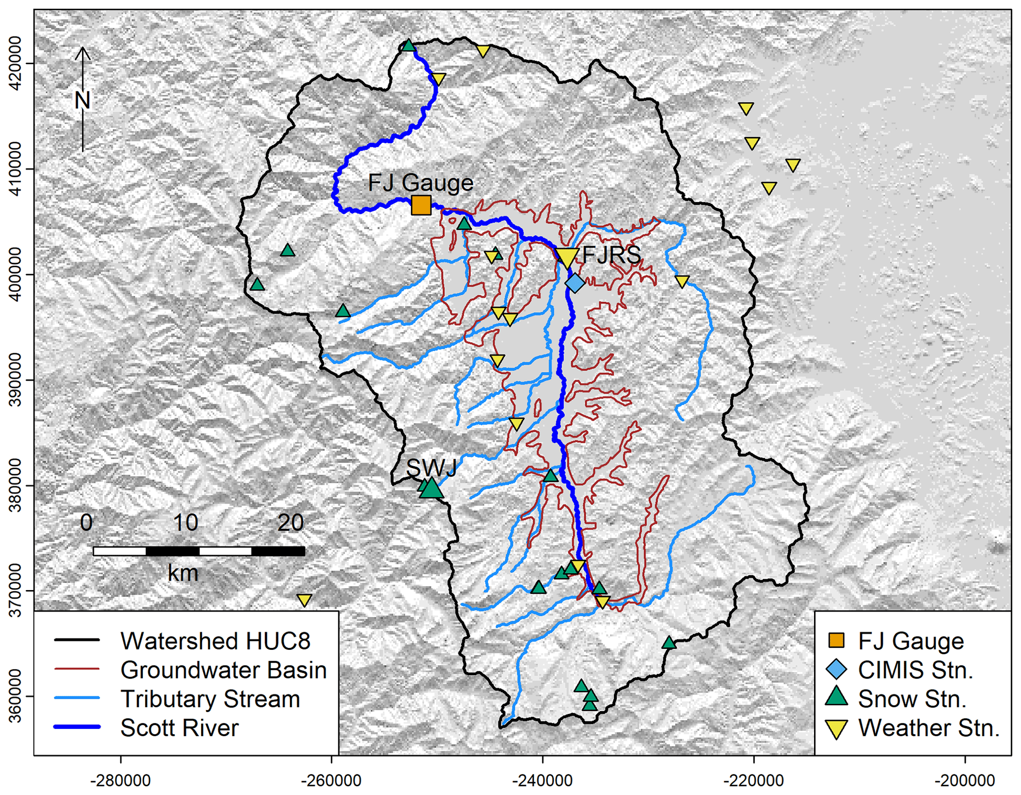
Figure 1 Scott River HUC8 watershed and groundwater basin boundaries, stream network, and key monitoring locations: the Fort Jones stream gauge (USGS ID 11519500), weather stations, snow observation locations, and a CIMIS station (used to estimate reference evapotranspiration). Selected locations are highlighted with an enlarged symbol and an abbreviated label.

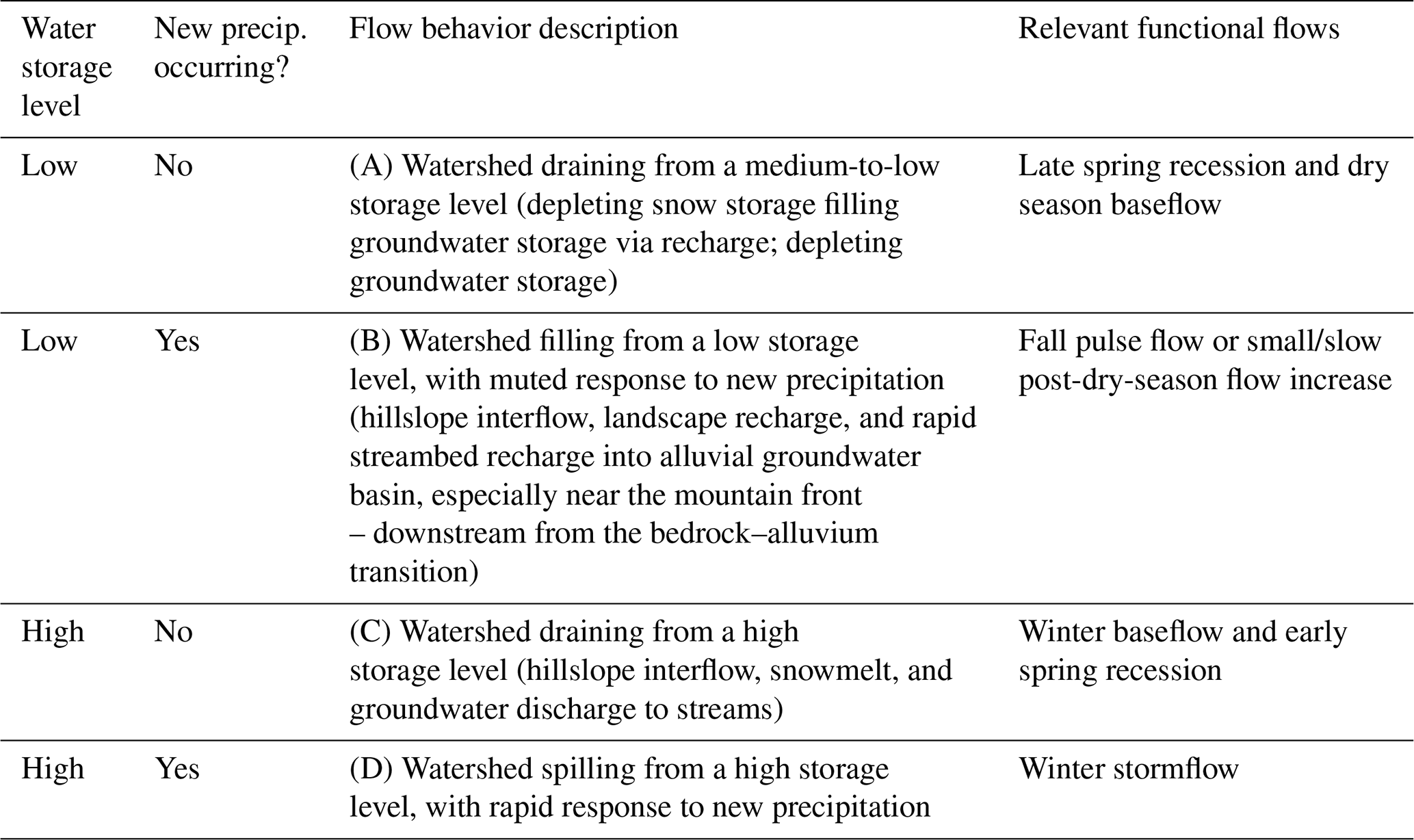
Figure 2 Illustration of four categories of Scott River watershed behavior. The hydrograph in the highlighted periods demonstrates the following watershed behavior: A, dry season baseflow – watershed draining from a medium-to-low storage level; B, moderate flow increase – muted flow surge response to new precipitation; C, winter baseflow and early spring recession – watershed draining from a high storage level; and D, winter stormflow – rapid flow surge response to new precipitation (storm spikes). Cumulative precipitation (right axis) is calculated using records from two regional weather stations; see Methods for details.

This study focuses on the transition from the dry season to the wet season, which at times can straddle the conventional water year boundary of 1 October, and cumulative precipitation is used both as a predictor and as a response variable (P_spill). When it is a predictor, a traditional 1 October start date is used and it is summed as the cumulative precipitation of October–April, to facilitate an end-of-April prediction of fall conditions. When it is the response variable, cumulative precipitation is counted starting on 1 September of the preceding water year, to capture uncommon September precipitation. This 1 September start date is also used in some graphs of climate and flow data (e.g., in Sect. 3.2 below) to establish and visualize baseline dry season conditions. Additionally, all flows in this study are observed or simulated at the USGS Fort Jones streamflow gauge (station 11519500), a key monitoring location downstream of nearly all water use and cultivated land in the HUC8 watershed (Fig. 1), with an observation record covering water year 1942–present day (USGS, 2023). (Data considered in this study extends to 30 September 2021.)

2.1 Scott River watershed precipitation-runoff behavior

To establish the context and hydrologic relevance of the two proposed predictive indices V_min and P_spill, a brief description of the behavior of the watershed is necessary. In an undammed catchment, the runoff response to one (or a series of) precipitation event(s) is dependent on multiple factors, including antecedent soil moisture conditions, the intensity and magnitude of the precipitation, and the dampening and delay of runoff; the latter is due to interflow, snow storage and recharge to groundwater storage that later returns as stream baseflow (Tarboton, 2003). A threshold runoff response to individual storm events has been observed at the hillslope scale where soil directly overlays (relatively) impermeable bedrock: absent significant aquifer storage, subsurface flow increases dramatically after a quantifiable threshold of precipitation is reached (Tromp-Van Meerveld and McDonnell, 2006). The proposed mechanism is the filling and connecting of various distributed storage volumes, such as soil pores and microtopographic relief in the bedrock surface (Tromp-Van Meerveld and McDonnell, 2006). Recently this concept has been extended to the watershed or basin scale: relative to the beginning of a storm event, a much higher flow response is possible only when a critical number of storage volumes throughout a basin fill to a threshold level and become connected (McDonnell et al., 2021).

In this study we expand this concept of a basin-scale, threshold-based runoff response to the temporal scale of a season, rather than a single storm event. In this framework the condition of the Scott River watershed, as measured at the basin scale using the Fort Jones stream gauge, can be classified into four main categories. These categories are distinguished by current precipitation conditions and the volumetric proportion of the hydrologically connected reservoirs that are full of water (Table 1).

Table 1 Watershed behavior and functional flow components occurring during the transition from the dry season to the wet season in a Mediterranean climate. The categories are illustrated in an example annual hydrograph in Fig. 2. Water storage level refers to the relative water content of the soil and aquifer within the watershed.

Water in the Scott River watershed is stored in five primary reservoirs (Harter and Hines, 2008):

• snowpack

• fractures in impermeable bedrock (uplands)

• soil moisture/subflow

• the alluvial groundwater aquifer (lowlands)

• streams and surface water bodies.

Accumulating snowpack is present only in the mountainous areas of the upper watershed and is limited to the winter and spring season. The alluvial aquifer is present only within the bounds of the groundwater basin underlying the flat valley floor. Water stored in fractured rock and soils/subflow emerges as springs in streambeds in the upper watershed (Fig. 1) (Mack, 1958). In conditions with sufficiently high soil water content or groundwater elevations, soil moisture/subflow and groundwater become hydrologically connected to the surface water system. Conversely, water in the snowpack and fractured rock reservoirs is not hydrologically connected to major surface water bodies until it melts or descends lower into the watershed, effectively passing through the aquifer or soil to reach the stream. For convenience the soil moisture/subflow and aquifer reservoirs will be referred to as “connected” storage. Storage in streams and surface water bodies is negligible at temporal scales exceeding a few days.

2.1.1 Rainfall-runoff response, functional flows, and Q_spill

In the absence of surface water reservoirs, it is useful to consider streamflow regimes from the perspective of natural water storage as an intermediary between precipitation and stream flow at the outlet of the watershed. At the end of the dry season, the watershed is in a “draining from low storage” condition: snow storage has not been available for several months and groundwater storage is reaching its annual low point. This is reflected in a slowly declining or flat hydrograph, with a flow rate that has decreased for several months (Fig. 2, first period A). As the dry season ends, the watershed begins receiving rain and enters a condition of “filling from a low storage level”. In this catchment, much of the earliest water entering the system is routed as recharge through the soil or the streambed to occupy space in the aquifer. Because groundwater moves more slowly through the watershed than surface water, the hydrograph at the Fort Jones gauge demonstrates a muted or delayed response to early rain events (Fig. 2, period B).

At the onset of a new wet season, under average conditions, the flow rate of filling is greater than the flow rate of draining, and therefore the “filling from a low storage level” condition at the beginning of a rainy season is transient, lasting only until the filling process occupies enough aquifer and soil storage volume to produce a “full” condition. After the water storage in the basin reaches “full”, if no more rain occurs, the watershed returns to its default “draining” condition, though from a higher storage baseline than during the dry season, and with a higher draining flow rate (Fig. 2, first period C). If there is additional precipitation, the resulting surge in flow is much more rapid, reflecting a “spilling” condition (Fig. 2, intermittent events D).

The precipitation and winter temperatures during the wet season produce an accumulation of snowpack, though in some years this can be reduced by warm periods and rain-on-snow events. Melting snowpack contributes subsurface flow and tributary streamflow to the lower watershed, producing a spring flow recession typically lasting from the last major precipitation event into the summer (Fig. 2, second period C and second period A) and providing significant recharge via stream leakage near the mountain front, at the margins of the alluvial basin. This process amounts to a net transfer of water in snow storage during winter and spring to water in groundwater storage in spring and summer.

Many of these phenomena are reflected in the well-established elements of functional flows (Table 1). Winter stormflow is the functional flow metric corresponding to a “spilling” watershed. The spring recession can last for 3–6 months and its steepness is moderated by snowmelt. Because it bridges the high-storage and low-storage states, the early and late spring recession appear in two different flow behavior categories (Table 1). Conversely, the flows that are here classified under “watershed filling from a low storage level” have no specifically discerning feature in the hydrograph and depend on year-to-year conditions. A discrete fall pulse flow does not occur in every water year, and no distinct metric has been proposed for the gradual post-dry-season flow increase.

Given the regular behavior observed during the dry season-to-wet season transition of the Fort Jones hydrograph (i.e., prolonged dry season baseflows followed by gradual flow increase and then storm surges), and the physical structure of this highly inter-connected basin, we propose that an operational flow rate threshold exists at the Fort Jones gauge that defines approximate transition to “full” or “spilling” basin condition (referred to here as Q_spill; see Results, Sect. 3.1).

2.1.2 Stream–aquifer interaction

In the groundwater basin (i.e., lower) portion of the watershed, the alluvial aquifer is the largest storage reservoir (Mack, 1958). Groundwater–surface water interactions drive Scott River flow behavior towards the end of the dry season, before the next rainy season begins, when snowpack is depleted and streamflow in many areas is sustained by groundwater discharge alone (Foglia et al., 2018). Discharge to streams from the alluvial aquifer occurs along the thalweg of the Scott River. In this highly interconnected system, groundwater discharge along the thalweg, at the annual scale, is balanced by landscape recharge and by recharge from stream reaches near the margins of the basin, overlying coarse alluvial fans (see discussion below).

We used the Scott Valley Integrated Hydrologic Model (SVIHM) (Tolley et al., 2019; Foglia et al., 2013a, b) to obtain the estimated volume of water exchanged monthly, in water years 1991–2018, between the surface stream network and the underlying aquifer. Streamflow gains from and streamflow losses to groundwater were integrated across the stream network to obtain a net monthly groundwater–surface water exchange value for the basin (Fig. 3a). These net monthly groundwater-to-stream flux values were then compared with simulated monthly flow volumes in the Scott River, measured at the Fort Jones gauge (Fig. 3b).

Figure 3 Both stream leakage and aquifer discharge increase in the rainy season, while net flux to the stream remains relatively close to 0 (a). Strong seasonal trends are evident in net flux to the stream (b; described further in Sect. 2.1.2).

2.2 Observed response variables (V_min and P_spill)

The Scott River is an undammed watershed in which estimates of annual precipitation are an order of magnitude greater than the estimated water pumped or diverted for agriculture (Tolley et al., 2019). In this study we tested whether fundamental hydrologic characteristics, specifically the dry season baseflow recession and the rainfall-runoff response to early wet season cumulative precipitation, can be predicted 5–6 months prior using observable hydroclimate data of the preceding wet season. The first step was to define and quantify relevant response variables describing these two processes.

2.2.1 Dry season baseflow quantities (V_min) and timing

Multiple integrated numerical indicators of dry season baseflows were evaluated for suitability as the response variables in this prediction exercise. Monthly flow volumes were preferred over a minimum daily flow value to reduce the influence of individual events, such as groundwater pumping or surface water diversions, that might affect flow for 1 d or a small number of days.

Historically, the rainy season in California tends to begin in October. By convention each water year begins on 1 October of the previous calendar year and ends on 30 September. Matching this convention, in most years, the minimum-flow month for the Scott River is September; however, uncommon September storms can elevate flow volumes, and in some years with a late rainy season onset, the October flow volume may be lower. To capture these dynamics, we calculated a rolling 30 d sum of daily flow volumes in the period July–December for each calendar year to identify the 30 d period with the least flow volume, referred to as V_min (see Sect. 3.2). For consistency, each annual V_min value was assigned to the water year ending in September of that calendar year, even if the minimum flow window included days in October–December of the following water year.

2.2.2 Cumulative precipitation P_spill

P_spill was calculated for each water year as the cumulative rainfall at the end of a dry season, between 1 September and the first day that the Fort Jones gauge measured flow greater than Q_spill (see Results, Sect. 3.2). As stated above, conceptually, it is the amount of rainfall needed to “fill” the watershed such that streamflow at the outlet of the watershed responds rapidly to new precipitation without significant intervening storage delays. A dry season can have negative effects on an aquatic ecosystem if it produces extraordinarily low flows, but also if it lasts for an extraordinarily long time (e.g., delayed salmon habitat access; CDFW, 2015).

In addition to the volumetric quantity P_spill, there could also be demand for seasonal predictions of the timing of onset of the coming rainy season. However, predicting the timing of the onset of the rainy season or of Q_spill would likely rely on uncertain long-term weather forecasts and is beyond the scope of this paper. In other words, due to randomness in rainfall timing, the exact dry season baseflow duration associated with a higher P_spill is highly variable and, hence, unpredictable.

2.3 Potential predictors and selected formulations

To evaluate candidate predictors of end-of-dry-season flow behavior, Pearson's correlation coefficient, R, was calculated between observed response variables V_min and P_spill, and the following categories of observed predictor data (see Results, Sect. 3.3):

1. Spring (March–May) water level observations in each of 54 individual wells within the study area (Fig. A1) (CNRA, 2019).

2. Annual maximum snowpack water content at 20 individual snow monitoring stations aggregated by the California Data Exchange Center (CDEC; Fig. 1) (CDEC, 2023).

3. Cumulative precipitation, October–April, at local weather stations (for this study area: 12 stations within and 5 outside the watershed for a total of 17 NOAA stations; Fig. 1). In these records, missing values (i.e., days with no recorded observation) are assumed to have 0 precipitation. Water years with more than 5 missing days are excluded from the predictor dataset (National Climatic Data Center et al., 2023).

4. Cumulative precipitation, October–April, of a composite precipitation record with no missing values, representing the mean of the Callahan and Fort Jones NOAA weather stations (located at the southern and northern ends of the valley, respectively) and referred to as “cal_fj_interp”. To generate the composite record, missing values in the Callahan and Fort Jones station records were calculated based on observations at neighboring stations (see method in Foglia et al., 2013a).

5. The flow volumes observed at the watershed outlet for this study area, referred to as the Fort Jones gauge (USGS ID 11519500; Fig. 1), during the preceding March and April (USGS, 2023).

6. Cumulative reference evapotranspiration (ET₀), October–April, here using observations from Station No. 225 in the California Information Management Information System (CIMIS) network (2015–2021), or Spatial CIMIS estimates of ET₀ at the location of Station 225 (2002–2015) (DWR, 2007, 2021) (Fig. 1).

7. The timing (in Julian days) of the date of maximum snowpack measurement.

8. The timing (in Julian days) of the date of the volumetric center of the rainy season, calculated as the day the cumulative precipitation crossed 50 % of the total.

9. The 1-year-lagged metrics of maximum snowpack, October–April cumulative precipitation, and April water levels (e.g., the October–April cumulative precipitation measured a full 17–23 months prior to a September minimum flow).

Individual measuring locations, such as wells or weather stations, were evaluated for sample size (i.e., years of data) and degree of relatedness with the two response variables. Relatedness of the monitoring locations with the highest R values in each category of monitoring observation are included in analysis results (see Results, Sect. 3.3).

2.3.1 Prediction formulae for V_min and P_spill

With a sample size of 80 years of dry season baseflow volumes, a one- or two-predictor model is best to avoid overfitting (James et al., 2013). Nonetheless, to thoroughly assess the predictive potential of this dataset, three-predictor models were also considered.

Commonly, model diagnostics such as Akaike's information criterion (AIC) are used to evaluate the best of a set of competing statistical models (Burnham and Anderson, 2004). However, AIC and other information criteria methods can only be used when comparing models based on the same dataset (Burnham and Anderson, 2004). In the dataset for this study, variable record lengths and missing data points produced a situation in which the sample size is different for most of the combinations of predictors under consideration. Consequently, though AIC and additional diagnostics were calculated for all models (Tables A1–A6 in the Supplement), cross-validation was used in this study as the primary model selection technique.

To predict V_min, a set of six one-predictor models were generated using the single observation location from each category with the highest R, and model fit was evaluated using Leave One Out Cross Validation (LOOCV) (see Results, Sect. 3.3; also see Table A1) (James et al., 2013). For a dataset with n observations, the LOOCV error of a predictive model is obtained by recalculating the model coefficients n times, each time leaving out one observation, and comparing the resulting prediction to the single left-out observation. The root mean square of these n errors is the LOOCV error used to evaluate model performance in Results.

The single predictors with the lowest LOOCV error (other than evapotranspiration of a reference crop, ET_ref, which was excluded due to insufficient observation record length) were used to produce a set of four two-predictor models (see Results, Sect. 3.4; also see Table A2) for V_min, including two that incorporate data from a full calendar year prior. A similar approach was used to assess two-predictor models for P_spill, though no predictors from a prior year were included, and several additional two-predictor combinations were evaluated. In both cases, the best-performing model took the following form:

$$\begin{array}{}\text{(1)}& {\mathrm{Predicted}}_i=\mathrm{Int}.+m_A\cdot {\mathrm{obs}}_{A,i}+m_B\cdot {\mathrm{obs}}_{B,i},\end{array}$$

where Predicted_i is the predicted value (either V_min or P_spill) in the calendar year i (i.e., at the end of water year i), obs_A,i, obs_B, i are the observed predictor values in October–April in water year i, and Int., m_A, and m_B are the coefficients of the selected linear model.

3 Results

3.1 Scott River precipitation-runoff behavior

The quantity P_spill is correlated with both a lower minimum flow volume and a later river reconnection (Fig. 4). This corroborates the hypothesis that P_spill is an indicator of the risk of a severe dry season.

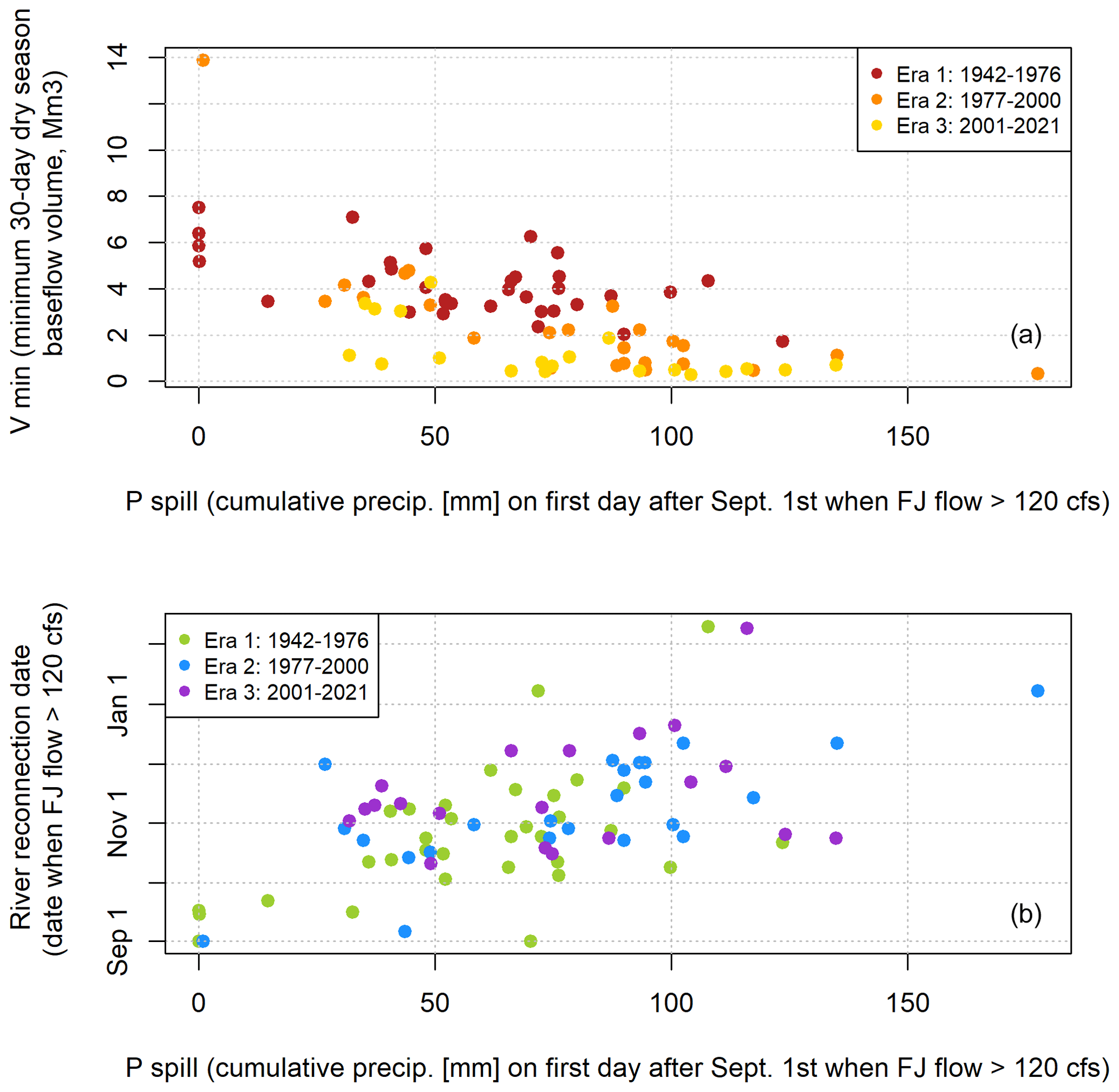
Figure 4 The quantity P spill (i.e., the amount of rainfall needed to “fill” the watershed such that it “spills” or responds rapidly to new precipitation) is correlated with both a lower minimum dry season baseflow volume (a) and a later date of river reconnection (b).

Visual inspection of 80 years of Fort Jones hydrograph behavior during the transition from the dry season to the rainy season (Fig. 5a) indicated that there were two distinct domains of flow: one in which flow is relatively flat (dry season baseflow); and one in which the flow rate is an order of magnitude higher, and it is highly responsive to rain events. The intermediate hydrologic state, “filling from low storage”, was visible in some fall–winter hydrographs (e.g., Fig. 2) but tended to last a relatively short time before the filling rate overwhelmed the draining rate and produced a responsive “spilling” condition.

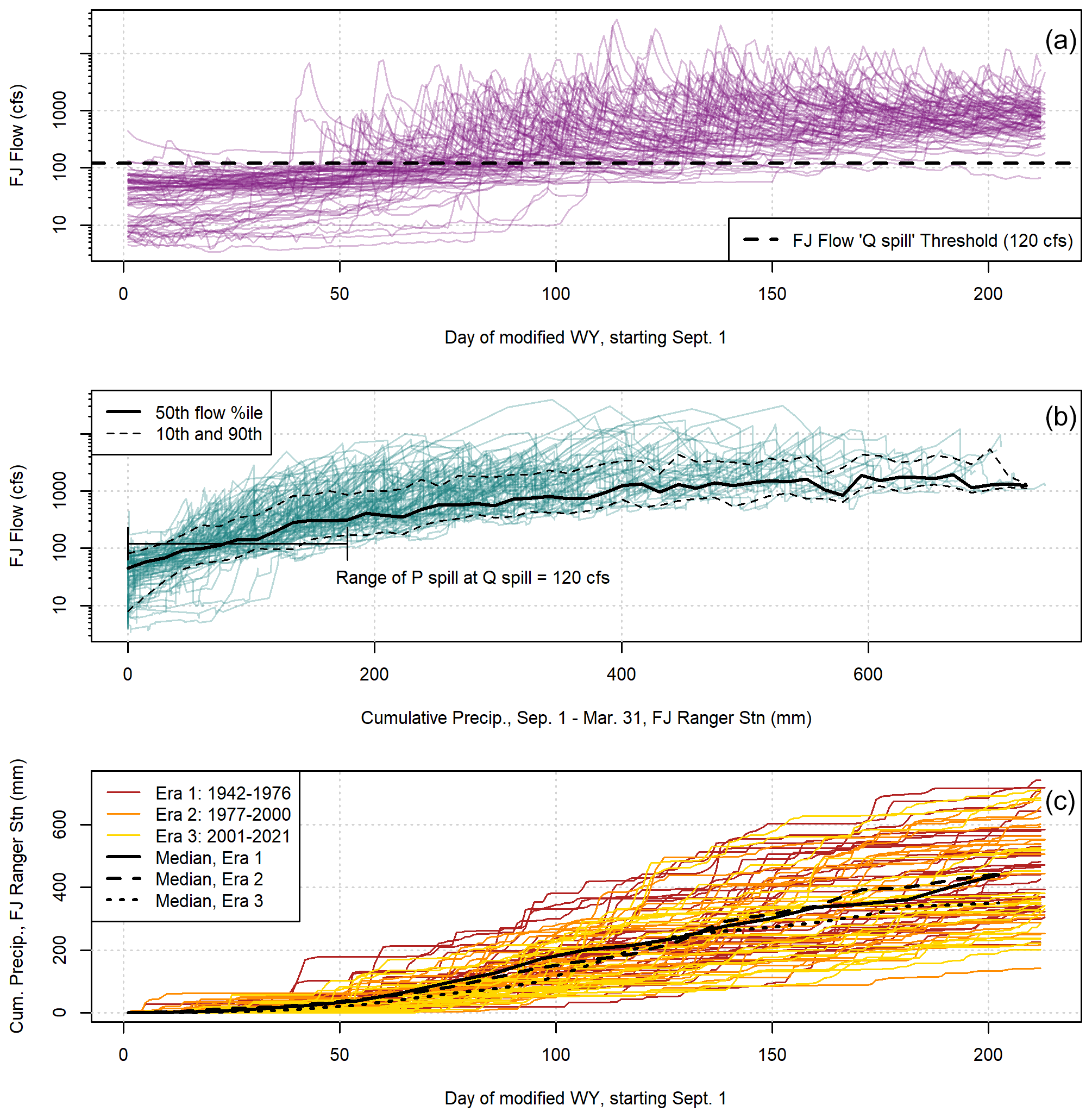
Figure 5 In all three panels, 80 years of data series from 1 September to 31 March are overplotted to illustrate dynamics during the transition from the dry to the wet season: observed Fort Jones hydrographs in (a), cumulative rainfall and Fort Jones flow values on fall and winter days in (b), and cumulative rainfall over time in (c).

The approximate threshold between these two hydrologic periods, denoted as Q_spill, was 120 cfs (294 000 m³ d⁻¹ or approximately ×10⁶ m³ per month). This value was determined by testing a range of potential Q_spill values to evaluate rainfall-runoff responses preceding and following the threshold (Fig. A2).

3.2 Observed response variables

3.2.1 Dry season baseflow quantity and timing

Minimum 30 d dry season baseflow volumes, denoted here as V_min, ranged from 0.3 to 7.5 Mm³ per 30 d (3.9–102 cfs), with one outlier value of 14 Mm³ per 30 d (189.2 cfs) in 1984 (see high V_min values in Figs. 4a and 6a), when an early September storm followed a wet year in 1983.

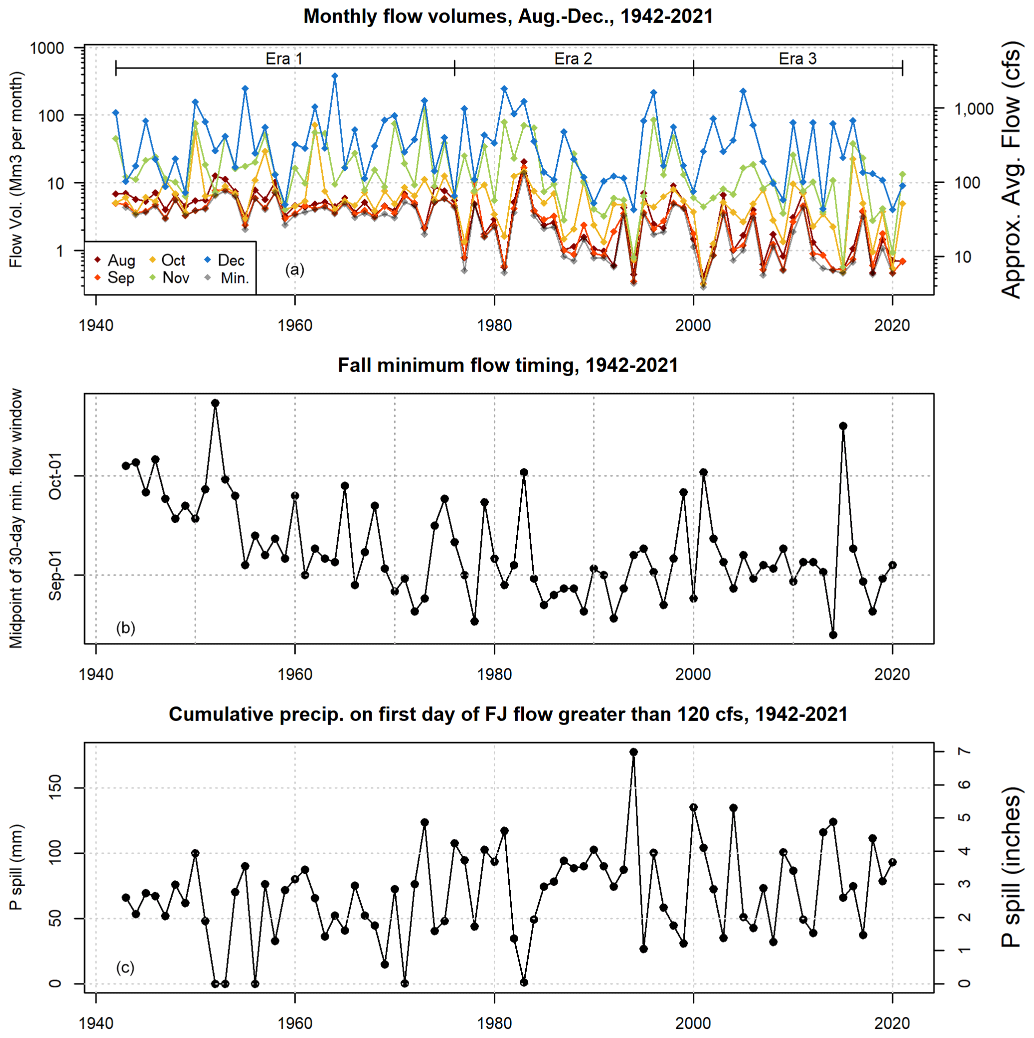
Figure 6 Panel (a) shows FJ gauge flow volume, by year, aggregated to monthly time windows in the late summer, fall, and early winter. Eras are noted that correspond to various management and climate factors. Panel (b) shows that the timing of dry season minimum flows has ranged from late August to mid-October over the past eight decades. Panel (c) shows that P_spill has trended upward over the period of record.

As mentioned previously, three eras have been proposed for the Scott River flow record: eras 1, 2, and 3, ranging from 1942 to 1976, 1977 to 2000, and 2001 to 2021, respectively. Matching other long-term declining flow trends in this watershed, the flows in August and September are relatively steady in era 1, and they become more variable with significantly lower lows in eras 2 and 3 (minima of 2.1, 0.35, and 0.33 Mm³ per 30 d or 28.6, 4.8, and 4.4 average cfs in eras 1, 2, and 3, respectively; Fig. 6a).

The timing of the midpoint of the 30 d minimum-flow period falls most commonly in September, though it has fluctuated over the past eight decades (Fig. 6b).

3.2.2 Cumulative fall precipitation and watershed response

Typically, flow at the Fort Jones gauge is low (i.e., less than the Q_spill threshold of 120 cfs) and stable through the end of the dry season (Fig. 5a). However, in some water years prior to the 1980s, the Fort Jones flow rate exceeded Q_spill on 1 September (Fig. 5a and b), indicating that even under persistent dry season draining conditions, under the climate and water use conditions of wet years in the mid-20th century, the Scott River remained responsive to new precipitation year-round. As a result, the range of P_spill, the cumulative precipitation necessary to reach Q_spill, is wide (0–178 mm, or 0–7 in.) (Fig. 6c). Mean P_spill values were 57, 79, and 76 mm (2.3, 3.1, and 3 in.) in eras 1, 2, and 3, respectively.

3.3 Comparison with California DWR water year type category

The California Department of Water Resources (DWR) water year type categories map well onto the two proposed hydrologic indices V_min and P_spill (Fig. 7a and b), which is to be expected, as both DWR WYT and the two proposed indices are based in part on cumulative precipitation data. However, there is less of an ability to identify a long-term trend in the DWR WYT index time series than in the time series of observed or predicted V_min or P_spill values. Likely causes of this difference include, first, the information lost when binning water years into five categories, and, secondly, the 30-year ranking window that would prevent a direct comparison of post-2000 WYTs with pre-1950s WYTs (Fig. 7c).

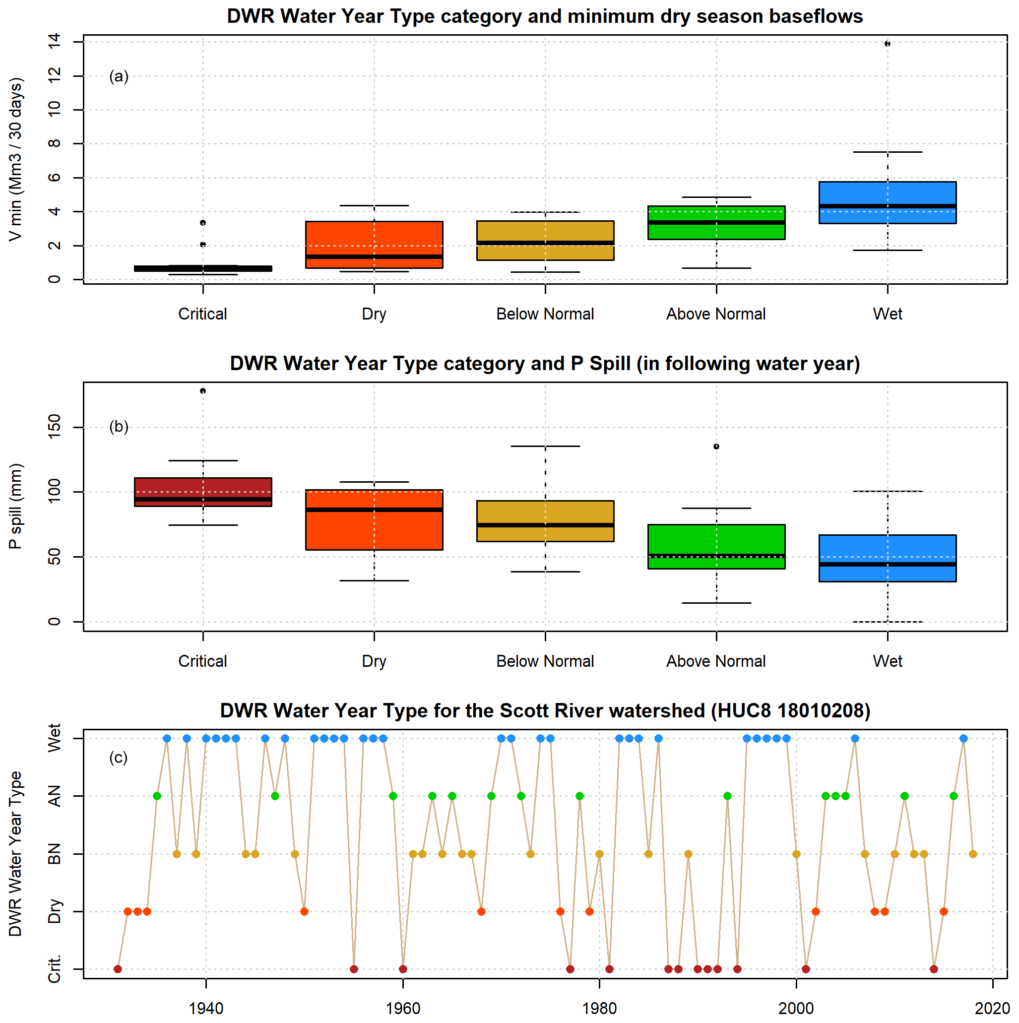
Figure 7 DWR water year type indices over time and compared with the two metrics of hydrologic conditions developed in this study: minimum 30 d dry season baseflow volume (V_min) and the amount of precipitation necessary to produce 120 cfs flow in the Scott River (P_spill).

3.4 Predictor comparison for V_min and P_spill

The observations of spring flows, snowpack, valley floor precipitation, and groundwater elevation are positively correlated both within each category and to each other overall (Fig. 8), which is unsurprising: wet years are associated with higher values in all of these categories. Groundwater wells with the highest predictive power tend to have long records (e.g., n of 10 years or more) and to be close to the Scott River. These results incorporate two wells proximate to the river, with record lengths of 43 and 57 years (Fig. A1).

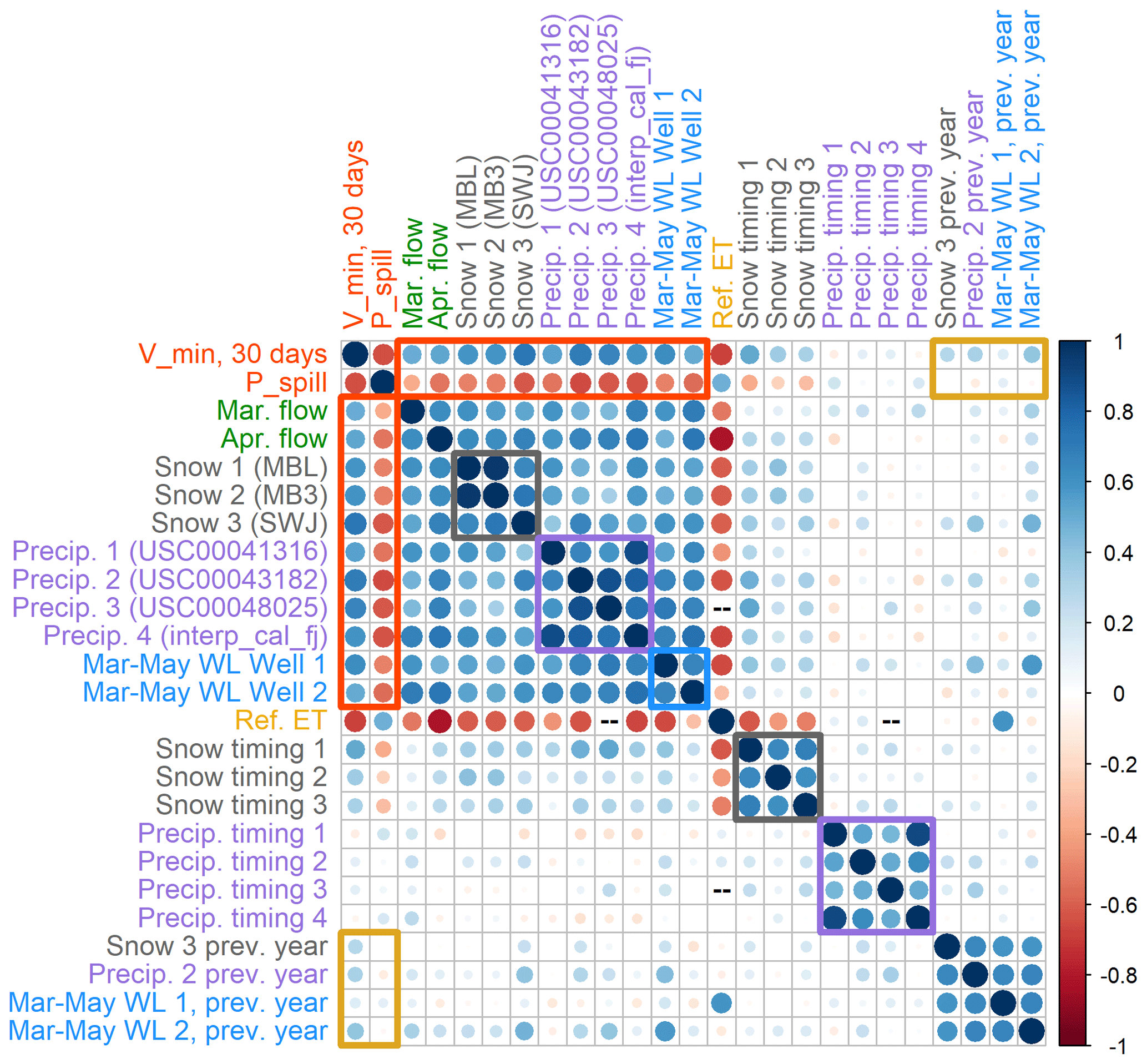
Figure 8 Correlation coefficient matrix of two response variables, minimum 30 d dry season baseflow volumes (V_min) and cumulative precipitation necessary to produce 120 cfs in the Scott River (P_spill), with various possible predictor metrics. Gray, purple, and blue squares highlight the inter-category correlation coefficients of snowpack metrics, October–April cumulative precipitation, and March–May groundwater elevation measurements. Red rectangles highlight the predictors with the greatest absolute correlation coefficient values with V_min and P_spill, respectively. Yellow rectangles highlight correlations with previous-year hydroclimate quantities.

Both response variables are correlated with four categories of observations: spring flow rates, maximum snow water content, cumulative precipitation recorded at weather stations on or near the valley floor (October–April), and March–May water levels in some wells. Observations in these categories are positively correlated with V_min and negatively correlated with P_spill. The correlation coefficient, R, of these response–predictor relationships range from 0.5 to 0.73 for V_min and from −0.38 to −0.66 for P_spill (Fig. 8).

In contrast to these four categories, October–April cumulative ET₀ is negatively correlated with V_min and positively correlated with P_spill (R of −0.68 and 0.48 for V_min and P_spill, respectively). October–April cumulative ET₀ is also negatively correlated with snow, precipitation, and groundwater level indicators. This could be because ET can remove a significant volume of water from the watershed, or because years with more rainy or stormy days accumulate less total insolation and atmospheric water demand. Additionally, the relatively high correlation (R) between ET₀ and the two response variables may be due to a small sample size, as all available ET₀ observations or estimates are from 2002 or later (i.e., in era 3; Fig. A3).

Some meteorological timing was evaluated in addition to quantities. Both response variables are moderately-to-weakly correlated with snow timing (i.e., the Julian day of the maximum measured snowpack in a given year; R of 0.33 to 0.52 and −0.22 to −0.384 for V_min and P_spill, respectively), but no significant correlation is evident between the response variables and precipitation timing (Fig. 8).

Finally, a subset of observations from the previous water year were included in the correlation matrix to test for multi-year influence on the response variables. These previous-year metrics had very little predictive power regarding minimum flows (correlated with V_min with an R of 0.29–0.33) and virtually none regarding P_spill (correlated with P_spill with an R of −0.01 to −0.1).

3.5 Predicted values of V_min

3.5.1 V_min predictor assessment and prediction formula

Six hydroclimate data categories contained at least one measurement station with an R value greater than 0.5 between a data record and observed V_min values. The single monitoring location in each of these categories with the highest R value was selected for further analysis (Fig. A3). (Although an R value of 0.5 is not considered a strong correlation on its own, it was selected as an inclusion threshold to retain any predictors that could provide useful information in combination with other predictors.) Out of this set of six hydroclimate data records, the maximum snowpack and October–April cumulative precipitation produce the lowest model errors (LOOCV errors of 2.74 and 2.72 Mm³, respectively; Fig. A3, top two panels; Table A1). Among combinations of two predictors, a linear combination of maximum snowpack and cumulative precipitation improved on the best single-predictor model, with an LOOCV error of 2.29 Mm³ (Fig. A4, upper left panel; Table A2). No three-predictor models produced lower LOOCV or higher R² values than the best two-predictor models (Table A3), so no visualizations were made of three-predictor model results.

Among the two-predictor models evaluated was a combination of maximum snowpack water content and the timing of the maximum measurement (Fig. A4, top right panel). This produced a slightly larger error (2.78 Mm³) than the single-predictor model with maximum snowpack water content alone (2.74 Mm³; Fig. A3, middle left panel), indicating that the timing of maximum snow accumulation is either relatively unimportant in generating dry season baseflows or that the actual timing of the snowpack maximum is not captured in temporally sparse snow course measurements.

Additionally, two models featuring a partial 1-year holdover were evaluated to test the validity of this component of the methodology of DWR's WYT index. In both cases, the addition of the climate data from the previous year produced a very small change in model error (Fig. A4, two lower panels), indicating that in the Scott Valley context, the previous year's climate may have a minor influence on dry season flows relative to the immediately preceding rainy season.

Based on these results, the model selected to provide the best V_min prediction formulation was a linear combination of the snowpack maximum from the Swampy John (SWJ) snow station (with data aggregated by CDEC) and cumulative October–April precipitation from the Fort Jones Ranger Station (FJRS) weather station (with data collected by NOAA) as follows:

$$\begin{array}{}\text{(2)}& V_{\min ,i}=-\mathrm{1.33}+\mathrm{0.0053}\cdot {\mathrm{FJRS}}_i+\mathrm{0.0027}\cdot {\mathrm{SWJ}}_i,\end{array}$$

where V_min,i is the predicted value of minimum 30 d dry season baseflows in the calendar year i (i.e., at the end of water year i) (million m³ or Mm³), SWJ_i is the maximum snow water content recorded at the Swampy John snow course (CDEC station ID SWJ or 285) in water year i (millimeters) and FJRS_i is the cumulative precipitation, recorded October–April of water year i, measured at the Fort Jones Ranger Station (NOAA station ID USC00043182) (millimeters).

Diagnostics for the linear regression models assessed in the V_min analysis are included in Figs. A3–A5 and Tables A1–A3.

3.5.2 Predicted and observed V_min over time

The V_min formulation proposed above predicts minimum 30 d dry season baseflows with a model error of 2.29 Mm³ per 30 d (31.2 cfs) and a root mean squared error of 1.4 Mm³ (19.4 cfs). This RMSE indicates substantial uncertainty in any single year's prediction: it corresponds to 49 % of the mean V_min value, 2.9 Mm³ (40 cfs).

Matching the historical trends of decreasing snowpack, the observed and predicted V_min values show a downward trend over time (Fig. A5, top panel). An outlier in 1984 reflects extremely high minimum dry season baseflows relative to the predicted values and the overall distribution. In that year, a relatively high-baseflow season was followed by an early September storm. The model residual (predicted minus observed flow volumes) for 1984 is also an outlier, indicating that the model has a sufficient sample size to not be overwhelmed by this extreme value produced by an exceedingly rare sequence of events (Fig. A5, middle panel).

The predictive V_min model is based on observations from the full record, but three additional models were generated based on only the observations from each period: eras 1, 2, and 3, respectively. Residuals based on era 1-data are similar to those of the full record, with a slight but systematic overprediction in era 3; era-2 residuals tend to overpredict in era 1 more than the full record; and era-3 residuals offer better performance in era 3 than the full record, but produce significant systematic underpredictions pre-2000 V_min values (Fig. A5, middle panel).

3.6 Predicted values of P_spill

3.6.1 P_spill predictor assessment and prediction formula

The two best single predictors of P_spill (with the largest R or least error, or both) were the October–April cumulative precipitation and the maximum snowpack (Fig. A6, top two panels), the same parameters that provided the best prediction for V_min. The LOOCV model errors are 850 and 718 mm, respectively. As in the V_min model development, ET₀ was excluded from consideration due to short record length. The best two-predictor model was the combination of the two best single predictors, with an LOOCV error of 697 mm (Fig. A7, upper left panel). No three-predictor models produced lower LOOCV or higher R² values (Table A6), so no visualizations were made of three-predictor model results.

Several combinations of correlated observation categories produced comparable model results, such as spring water levels with maximum snow, maximum snow timing, and cumulative precipitation (Fig. A7, upper right and two middle panels). However, not all combinations of co-correlated data produced reasonable predictions: a model with a linear combination of maximum snowpack timing and March flow volumes performed relatively poorly (LOOCV error of 1087 mm; Fig. A7, lower right panel).

Based on these results, the model selected as the P_spill formulation for a given water year was a linear combination of the same observation records as V_min, i.e., the snowpack maximum from the SWJ snow station (with data collected by CDEC) and cumulative October–April precipitation from the Fort Jones Ranger Station weather station (station ID USC00043182, with data collected by NOAA):

$$\begin{array}{}\text{(3)}& P_{\mathrm{spill},i}=\mathrm{128}-\mathrm{0.095}\cdot {\mathrm{FJRS}}_i-\mathrm{0.028}\cdot {\mathrm{SWJ}}_i,\end{array}$$

where P_spill,i is the predicted value of cumulative rainfall at the end of the dry season, starting 1 September, on the first day that the Fort Jones gauge records flow greater than or equal to 120 cfs in the calendar year i (i.e., at the end of water year i) (millimeters); SWJ_i is the maximum snow water content recorded at the Swampy John snow course (CDEC station ID SWJ or 285) in water year i (millimeters); and FJRS_i is the cumulative precipitation, recorded October–April of water year i, measured at the Fort Jones Ranger Station (NOAA station ID USC00043182) (millimeters).

Diagnostics for the linear regression models assessed in the P_spill analysis are included in Figs. A6–A8 and Tables A4–A6).

3.6.2 Predicted and observed P_spill over time

The P_spill estimate formulation proposed above predicts P_spill values with a model LOOCV error of 697 mm (27.4 in.) and a root mean squared error of 25.4 mm (1 in.). This RMSE indicates substantial uncertainty in any single year's prediction: it corresponds to 37 % of the mean P_spill value, 68.8 mm.

Matching the historical trends of decreasing snowpack, the observed and predicted P_spill values show an increasing trend over time (Fig. A8, top panel). A high outlier in calendar year 1994 (in early water year 1995) was caused by a dry water year 1994 followed by a series of small storms in November and December, none of which produced 120 cfs of flow, followed by a much larger storm on 8–9 January 1995 in which the river flow jumped to 600 and then 7500 cfs over 48 h.

The predictive P_spill model is based on observations from the full record. As in the analysis for V_min, three additional models were generated based on only the observations from each period: eras 1, 2, and 3, respectively. Residuals based on era 1 tend to underpredict eras 2 and 3 more than the full-record model, era-2 residuals tend to overpredict in eras 1 and 3 more than the full record, and era-3 residuals have a slightly higher tendency to underpredict than the full record but overall are fairly similar to the full-record residuals (Fig. A5, lower panel).

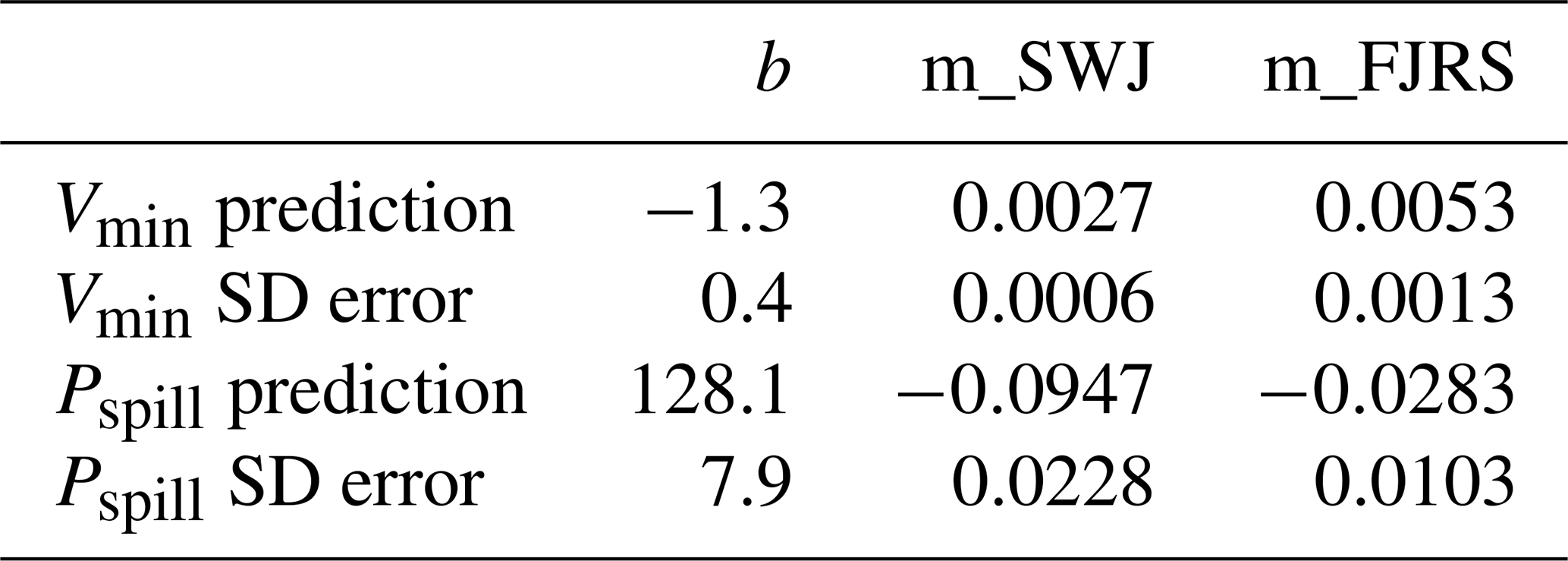
The linear coefficients for the two prediction equations and their standard errors are summarized in Table 2.

Table 2 Summary of linear model coefficients for V_min and P_spill.

4 Discussion

4.1 Scott River watershed behavior and long-term planning

The forward-looking seasonal predictions in this study are possible because of predictable hydrologic relationships between early-season inputs (precipitation) and late-season outputs (surface flow and ET), as is typical for many Mediterranean climate watersheds. In this watershed there are reasonably consistent rainfall-runoff relationships: the general shape of the relationship between cumulative precipitation and river flow at onset of the rainy season is preserved in dry and wet water years (Fig. 5b). This consistency is also reflected in stormflow behavior occurring after precipitation fills the watershed, a condition in which the Scott River exceeds a flow rate of Q_spill at the Fort Jones stream gauge.

A Q_spill threshold of 120 cfs was identified by an analysis of rainfall-runoff responses and a visual inspection of fall hydrograph behavior (Figs. 5 and A2). It also matches information from local stakeholders. Many tributary streams on the valley floor run dry during the summer and fall, and some tributary streams respond more quickly to fall precipitation than others. Generally, the timing of all tributaries reaching flowing status corresponds with the Fort Jones gauge reaching approximately 100 cfs (Sari Sommarstrom, personal communication, 2020).

Simulated estimates of stream–aquifer exchange corroborate these precipitation–flow relationships. Dry season baseflow (V_min) and the onset of wet season flow (framed in terms of P_spill) are both influenced by net groundwater discharge from the aquifer. One interpretation of the high frequency of near-0 net monthly stream–aquifer flux values (Fig. 3b) is that the high degree of connectivity between the streams and the aquifer in the Scott River system produces balancing counter-forces, such as large recharge events, in response to hydrologic stresses on the system. This balancing tendency can be temporarily overwhelmed by large precipitation pulses, but high-flow conditions quickly reduce the volume of water in the surface water system, returning the Scott River to a baseline of relatively balanced stream-to-aquifer and aquifer-to-stream fluxes. This dynamic also reflects the small size of the available aquifer storage relative to the amount of precipitation received by the watershed in a given water year (California DWR, 2004), leading to net groundwater contributions that are one to two orders of magnitude smaller than streamflow during “spilling” conditions (Fig. 3b) and two or more orders of magnitude difference between dry season low flows (almost exclusively from groundwater contributions) and wet season high flows.

These limitations in natural water storage substantially reduce the potential to use wet year surplus water for dry years. These results suggest it would be most productive to focus on within-year projects and management actions that either carry over some of the wet season flow to enhance dry season flow (V_min), and possibly reduce P_spill via interim aquifer storage, or that reduce surface water diversions and groundwater pumping, or a combination of both. These conditions also reduce resiliency to climate change.

4.2 V_min and P_spill prediction utility

Though various methods exist to qualitatively predict, in the spring, the severity of the coming low-flow season in the Scott River watershed, a quantitative short-term forecasting index could support more rigorous thresholds for adaptive management. To this end we developed two linear equations for predicting minimum dry season baseflows about 5 months in advance, by taking an inventory of relevant seasonal hydrologic inputs in April. The V_min and P_spill predictions could be used to support decision-making processes in the late spring time frame on potential regulatory actions and cropping decisions affecting the growing season.

There are several methods in current use. Observations at existing monitoring locations, such as weather stations and long-term snow course records, have been used as ad-hoc hydrologic indices. Historical adaptive management decisions in the Scott River watershed, such as planning to purchase surface water rights leases, have relied on individual monitoring observations, such as percent of snowpack relative to average conditions, or the Fort Jones flow in the spring (e.g., SRWT, 2018). Additionally, DWR has effectively extended the methodology of the SVI and SJI metrics to all of California by publishing a categorical water year type (WYT) index for all its major watersheds (to the HUC8 level) (California DWR, 2021). This metric quantifies meteoric drought and relies only on precipitation data, so as to be comparable across the state. Matching SVI and SJI methodology, it can be calculated at multiple points in each spring, with a final determination in May, but in the case of Scott Valley it has been used to classify WYTs only retroactively through 2018. As previously mentioned, it is a relatively complex metric with provisions including a partial 1-year holdover (i.e., dry conditions in the previous year will make a dry-type categorization more likely the following year), and non-stationary index thresholds, with a 30-year ranking window.

The quantitative prediction methods proposed in this study map well onto the existing DWR WYT index (Fig. 7), which serves as a validation of this approach. However, the V_min and P_spill metrics preserve more detail. The primary advantages of the proposed method over the DWR WYT and other previous methods of gauging near-term hydrologic conditions is that it is tailored to local hydroclimate data and is interpretable as a numeric prediction of fall streamflow conditions. This could be used to inform regulatory actions that increase fall environmental flows, or – for surface water diverters – to plan for low-flow conditions. However, each seasonal prediction should be accompanied by its measure of uncertainty: the RMSE of this predictive model is 1.4 Mm³ (19.4 cfs), which is 49 % of the mean value for V_min, 2.9 Mm³ (40 cfs).

Though it also serves as an indication of the severity of a water year, the immediate seasonal utility of the second predicted metric, P_spill, may be less than for that of minimum dry season baseflows. Management decisions, such as the last possible date to keep a temporary stream gauge installed in a river without risk of it being washed out, could be informed by a P_spill prediction when combined with weather forecasts in the fall. This prediction also carries substantial uncertainty (RMSE of 25.4 mm (1 in.), which is 37 % of the mean P_spill value, 68.8 mm).

4.3 Management implications of best-performing predictors

As described in Results, the linear models that best predicted observed values of V_min and P_spill were both based on the same two observation locations (the SWJ snow course and the FJRS weather station; Fig. 1), both with lengthy observation records. One interpretation of these results is that the climate inputs produce a predictable fall watershed response, and that human management decisions have a negligible influence on fall river flow. However, model simulations suggest that the timing and magnitude of fall flow increases can be meaningfully influenced by human water use (e.g., scenarios in the Siskiyou County GSP) (Siskiyou County Flood Control and Water Conservation District, 2021).

Multiple possible explanations could reconcile these two pieces of seemingly contradictory evidence. First, random variability in human water use could be a contributing factor to the error of the predictive models of fall-season hydrologic behavior. Alternatively, human water uses could be so consistent in response to wet or dry season conditions that these water uses could be implicitly incorporated into the predictive models. If adaptive management actions (potentially including events as diverse as regulatory curtailments or individual cropping choices) are carefully recorded in the future, they could be compared with residuals of the climate-based predictive models to evaluate whether any signal of a response to human interventions can be observed.

Potentially, these seasonal predictions could be extended to additional watersheds (albeit ones with abundant available hydroclimate data). However, the feasibility of this geographic generalization is beyond the scope of this study and should be investigated in future work.

4.4 Influences of climate change on predictive indices

Both predictions (using the full record of hydrologic data) assume some degree of hydroclimate stationarity, in that they use historical snowpack- and precipitation-runoff relationships to predict modern runoff. In one sense, a longer-term record can be an asset, in that it provides context for the severity of the dry periods of the past two decades. In another sense it is a liability for prediction accuracy: for example, the predicted V_min values based on the full record appear to systematically overpredict V_min in the most recent era (2001–2021; Fig. A4, top left panel; Fig. A5, middle panel). This suggests that factors not captured in these climate data, such as warmer air temperatures, changing upland vegetation, and evapotranspiration dynamics, and possibly unknown changes in water use, may be altering the relationship between the spring water supply and dry season baseflow rates. However, even with detailed records of water use and management actions, disentangling the influences of hydroclimate and human management on streamflow conditions remains a complex challenge.

5 Conclusions

This study proposed two locally tailored hydrologic decision-support metrics for the Scott River watershed in northern California. Both metrics have been shown to be predictable quantities using snowpack and cumulative precipitation data from October to April: the first metric is the minimum 30 d flow volume in a given water year, referred to as V_min, which typically occurs in September or October. The second metric is the cumulative rainfall needed to “fill” the watershed after the end of the dry season to a “spilling” condition that responds quickly to precipitation events, referred to as P_spill. Both predictive indices can be calculated at the end of April to support near-term (seasonal) adaptive management regarding the growing season (summer through fall), similar to the SVI and SJI in California's Central Valley and other indices used throughout the western United States. However, climate change may reduce the predictive accuracy of indices based on long-term data records, and updates based on smaller numbers of more recent water years should be considered periodically.

The management choices facing local managers in this basin are difficult to quantify and summarize, as is the case in basins throughout the western United States and other semi-arid and arid regions globally. Locally derived summary metrics, tailored to regional hydrologic dynamics, have provided and will continue to provide tools for supporting those choices and communicating them to diverse stakeholders and the general public.

Appendix A: Well locations, Q_spill threshold selection and linear model diagnostics

A1 Groundwater well data

Groundwater elevation measurements collected in the spring were evaluated as a potential predictor of river flow behavior the following fall. The length of the records and number of spring-season measurements were variable, limiting the number of wells that could be used as predictor sites. Two wells were selected for the final predictor evaluation.

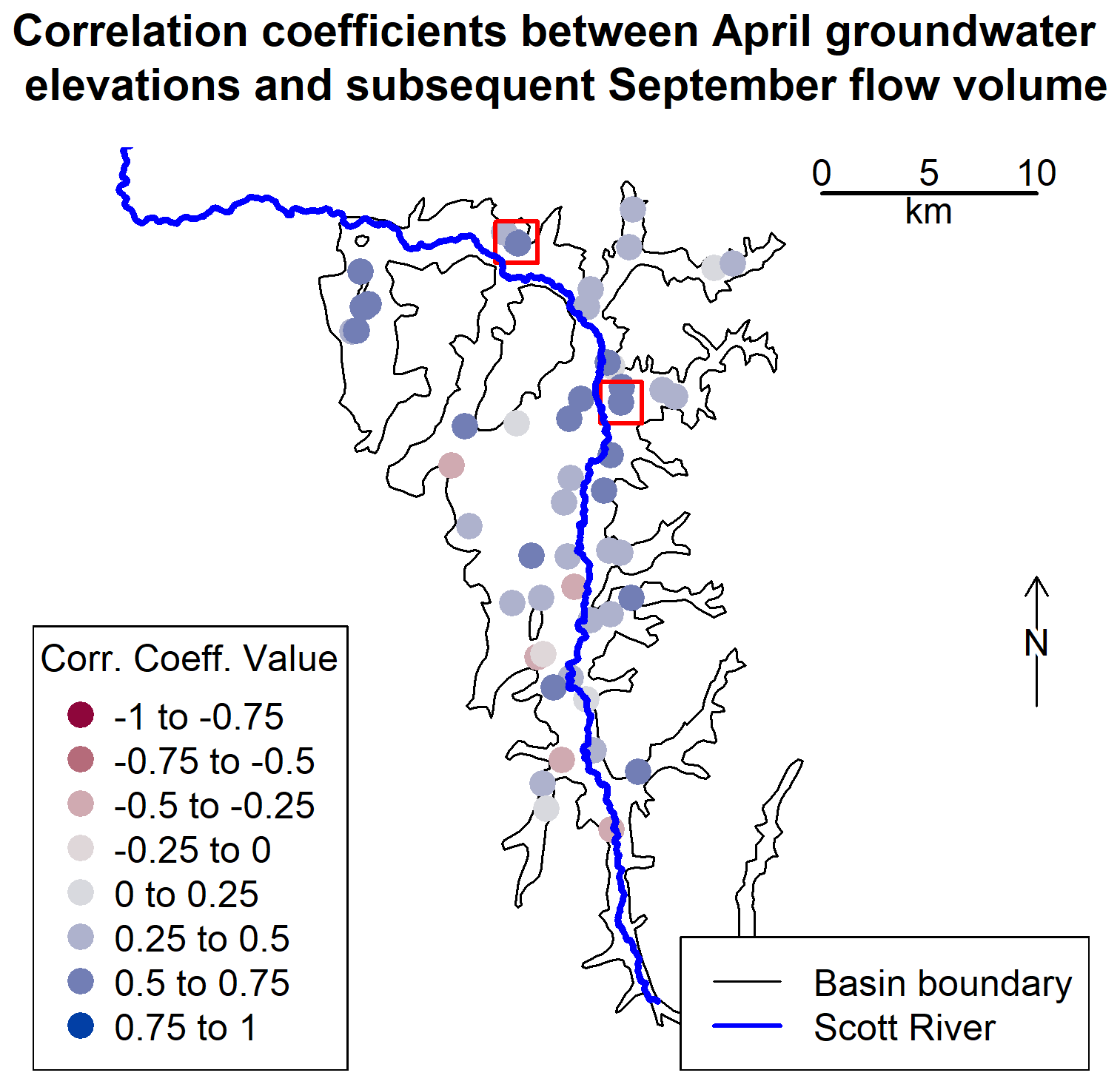
Figure A1 Boundary of the groundwater basin (corresponding approximately to the extent of the flat valley floor in the Scott River watershed) and selected well locations. Colors correspond to the correlation coefficients between April groundwater elevations and September flow volume. The wells included in the predictor comparison are highlighted with a red outer square. Fifty-four wells had enough spring-season water level measurements to be included in this correlation exercise, though some wells are so close together that their symbols overlap on this map.

A2 Selection of the Q_spill threshold value

The Q_spill value of 120 cfs (294 000 m³ d⁻¹ or approximately 9 Mm³ per month) was determined by testing a range of potential Q_spill values (10–500 cfs (24 000 to 1.223 ×10⁶ m³ d⁻¹)) as a dividing threshold between dry- and wet season flow behavior. Specifically, the threshold, Q_spill, was here operationally defined as the flow rate that generated the largest difference in rainfall-runoff response on either side of the dry season–wet season divide (Fig. A2a). The rainfall-runoff response was measured as the ratio $\mathrm{d}Q/\mathrm{d}P$, where dQ is the change in runoff and dP is the cumulative precipitation over the same moving 30 d period. Hence, the objective of this analysis was to find Q_spill such that the difference between the two $\mathrm{d}Q/\mathrm{d}P$ values for the 30 d immediately prior to reaching Q_spill and the 30 d immediately following the day when Q_spill reaches an initial maximum.

For the Scott Valley watershed, the difference between the wet and dry season rainfall-runoff responses reaches an initial plateau (113 cfs (275 m³ d⁻¹) of increased flow per millimeter of precipitation) for spill thresholds from 105–135 cfs (256–330×10³ m³ d⁻¹) (Fig. A2a). This indicates that in a large number of water years, flows in the range of 105–135 cfs (257–330 000 m³ d⁻¹) range are preceded by a dry season flow-response regime and followed by a distinct, flashier flow regime. Though higher wet–dry flow response differences were calculated at higher threshold values (i.e., up to 500 cfs (1.223 ×10⁶ m³ d⁻¹)), these progressively higher wet season flow responses likely reflect the falling limb of individual large storms that over-fill the watershed rather than separating filling from spilling behavior.

Additionally, in visual inspection of 78 years of Fort Jones hydrographs, the 120 cfs (294×10³ m³ d⁻¹) Q_spill threshold generated a plausible breakpoint between dry and wet season river behavior in all water years (e.g., water year 2016 in Fig. A2b). Furthermore, this value corroborates local observations that a value of approximately 100 cfs represents “fully connected” river conditions (see Discussion section).

A3 Model selection criteria: V_min

Diagnostics used to select the predictive models for V_min are shown below and discussed in Results. Predictors are abbreviated in tables and described briefly in Table A1. (For more information on potential predictors see Sect. 2.3.)

A4 Model selection criteria: P_spill

Diagnostics used to select the predictive models for P_spill are shown below and discussed in Results. Predictors are abbreviated in tables and described briefly in Table A4. (For more information on potential predictors see Sect. 2.3.)

A5 Diagnostic plots for selected models

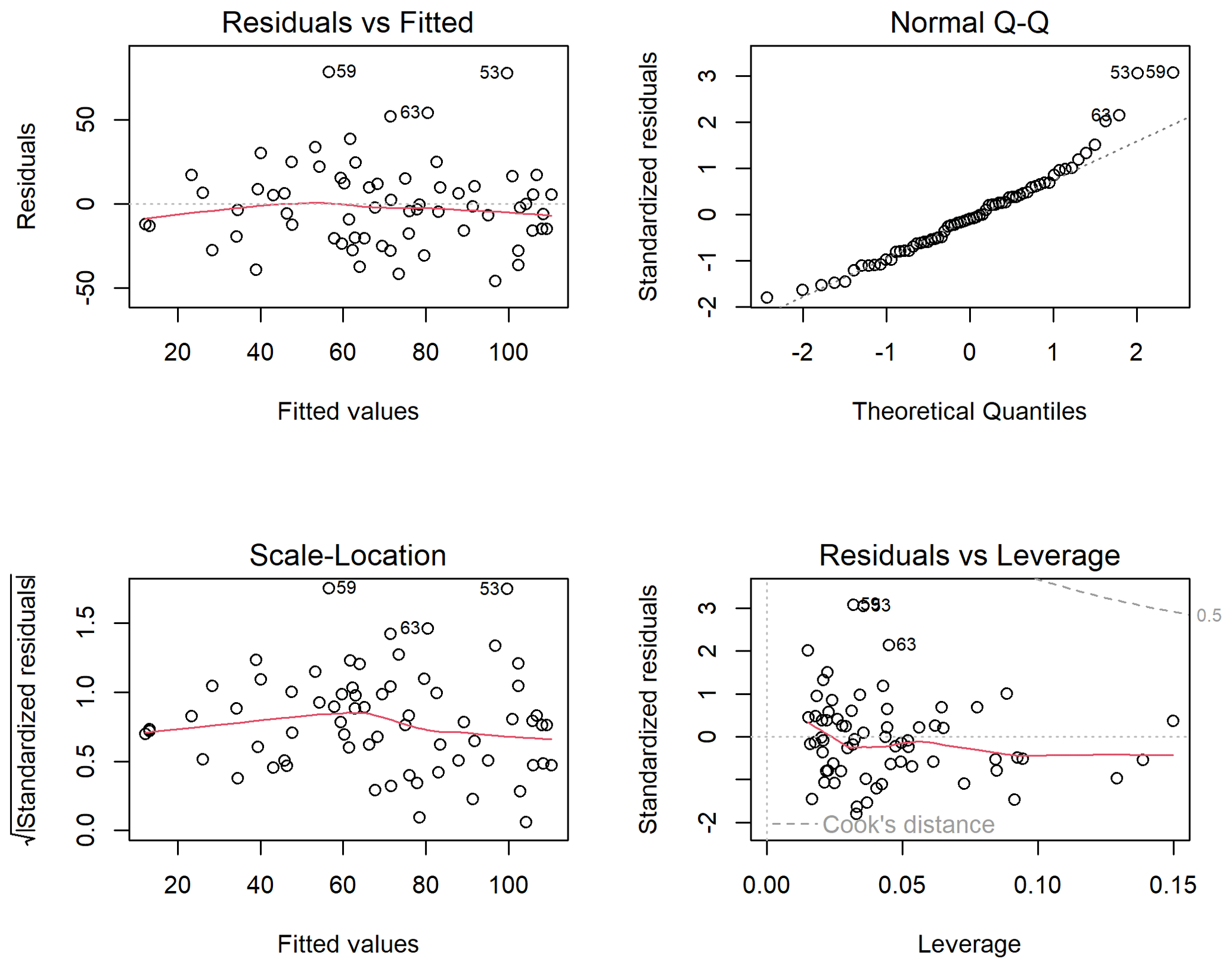
Standard diagnostic plots for the selected predictive models for V_min and P_spill. For V_min, these diagnostic plots highlight outlier record 42, which corresponds to the year 1983, when an early September storm followed a wet year. For P_spill, three lesser outliers are highlighted, corresponding to water years 1994, 2000, and 2004, in which the three highest values of P_spill were observed. These outliers represent the basin in extreme hydrologic conditions, so they are retained in the dataset even though they exert disproportionate leverage over the predictive models.

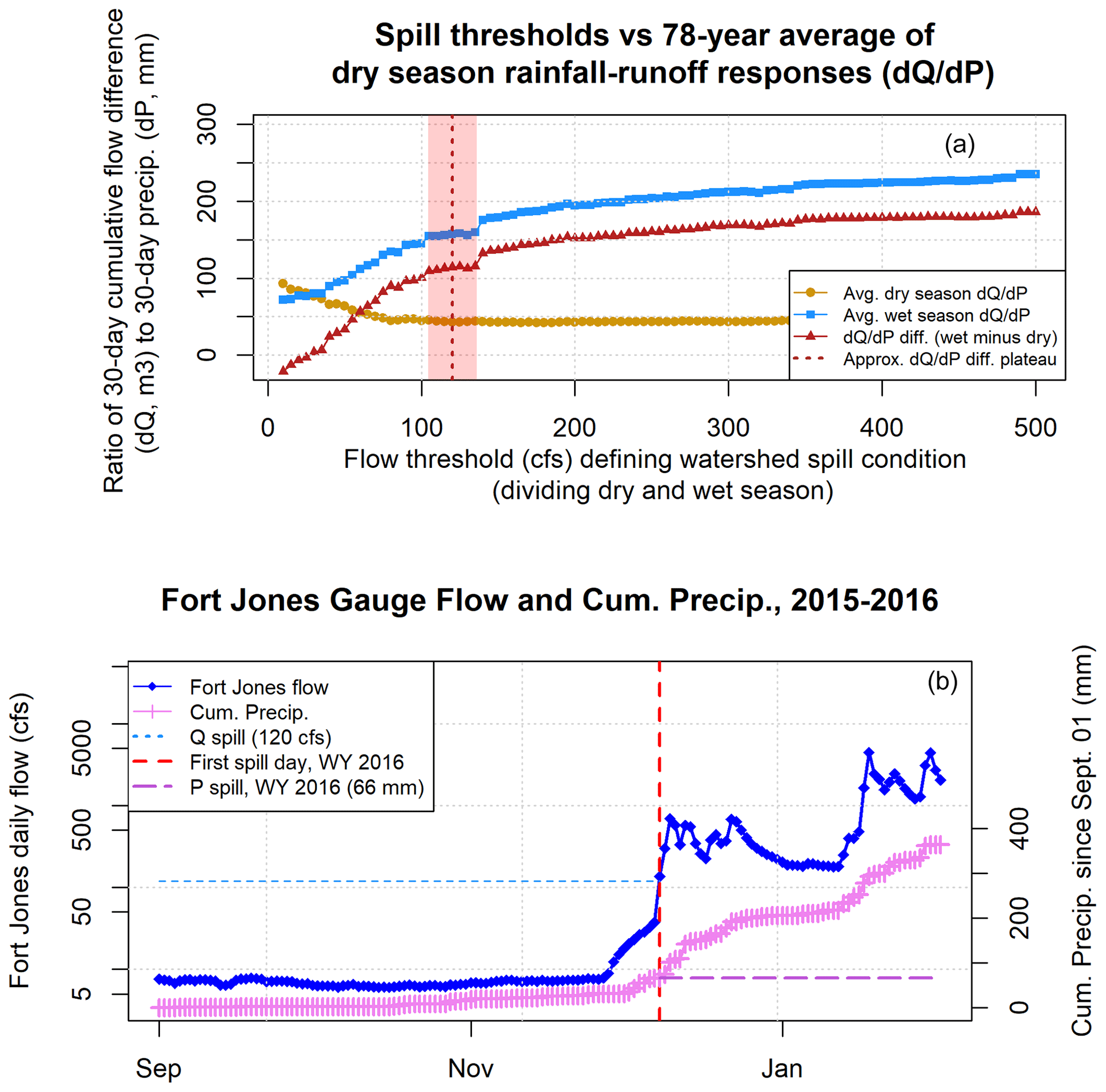
Figure A2 This analysis (a) aimed to identify the flow threshold that approximately defines the boundary between filling (i.e., dry season) and spilling (i.e., wet season) flow behavior at the Fort Jones gauge. For each threshold value (0–500 cfs) and for each water year, a rainfall-runoff response was calculated before and after the flow threshold. The rainfall-runoff response consisted of the 30 d cumulative flow difference (dQ) per 30 d cumulative rainfall difference (dP). A threshold value of 120 cfs was selected (see details in Sect. A2). In panel (b) the threshold is used to separate dry and wet season flow behavior in an example water year.

Table A1 Linear model diagnostics for one-predictor models of minimum fall flows (V_min).

Figure A3 Single-predictor models of minimum 30 d dry season baseflows in the Scott River.

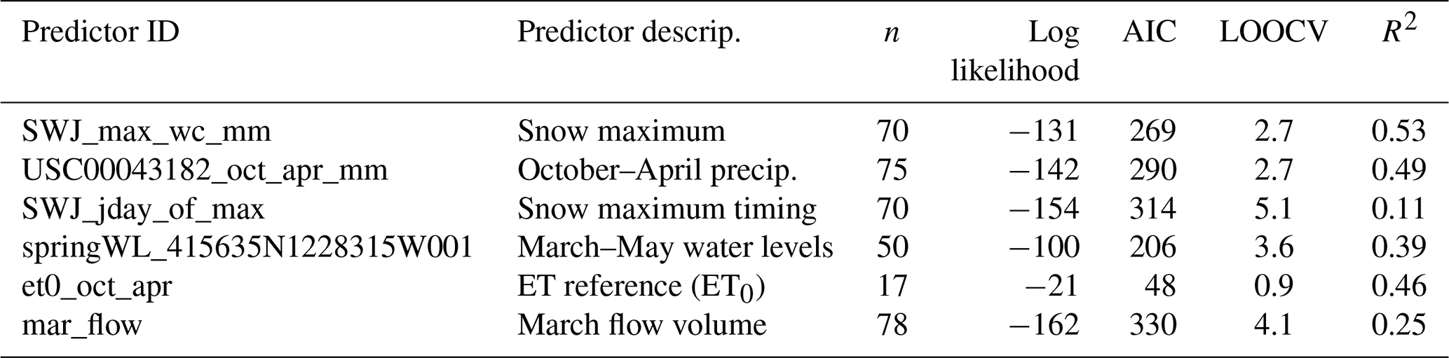
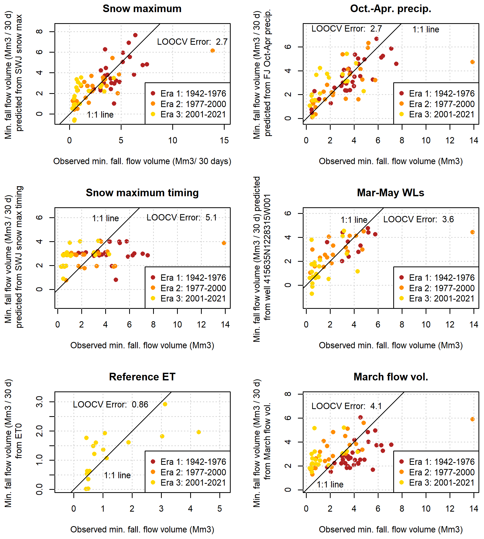
Table A2 Linear model diagnostics for two-predictor models of V_min. Reference ET was not included in two- and three-predictor models due to an insufficient sample size. (See Table A1 for description of predictor IDs.)

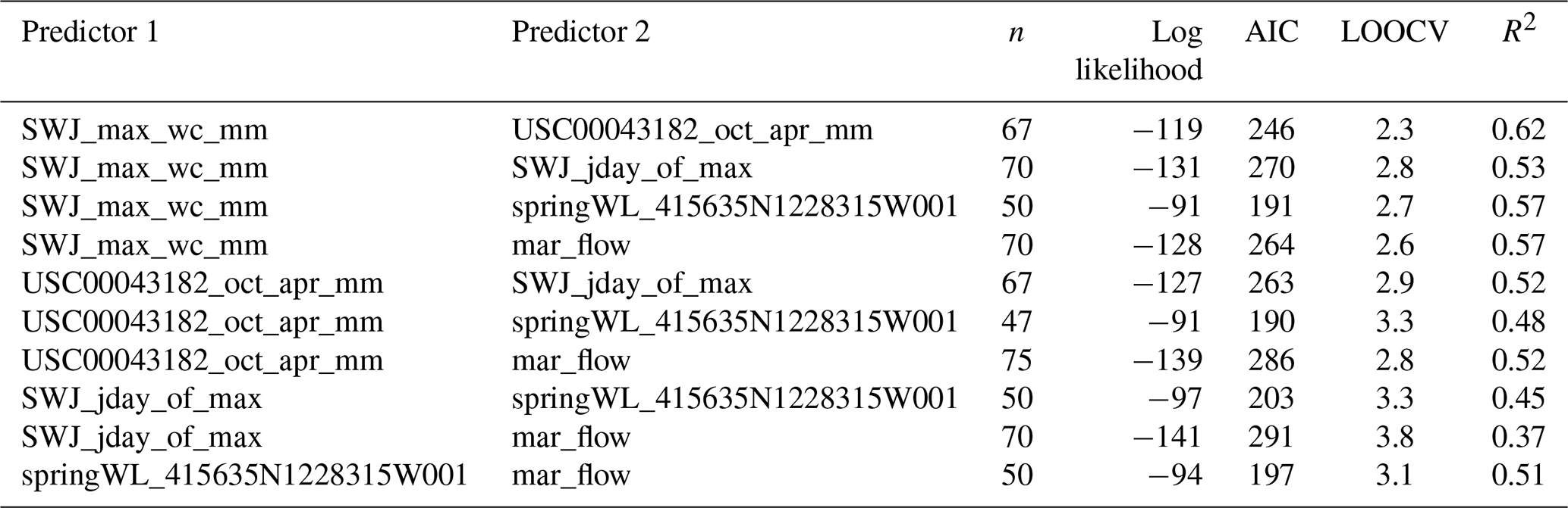
Table A3 Linear model diagnostics for three-predictor models of minimum fall flows (V_min). Reference ET was not included in two- and three-predictor models due to an insufficient sample size. (See Table A1 for description of predictor IDs.)

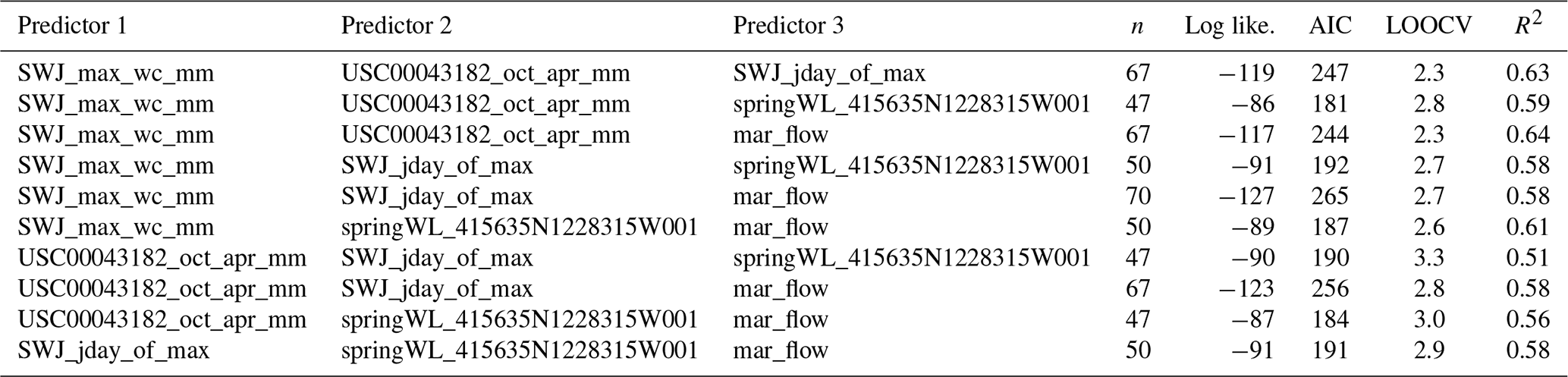
Table A4 Linear model diagnostics for one-predictor models of P_spill.

Figure A4 Two-predictor models of minimum 30 d dry season baseflows in the Scott River.

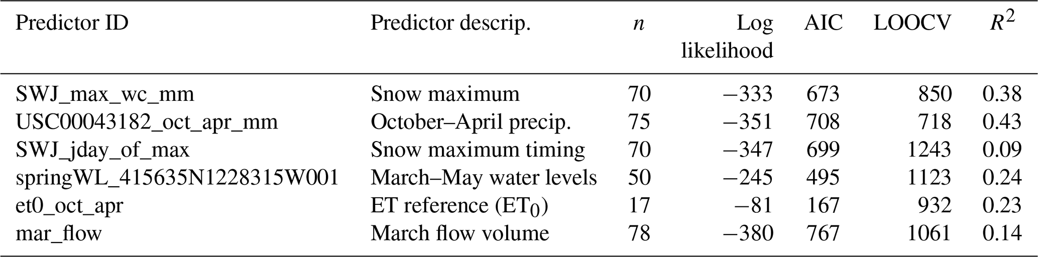
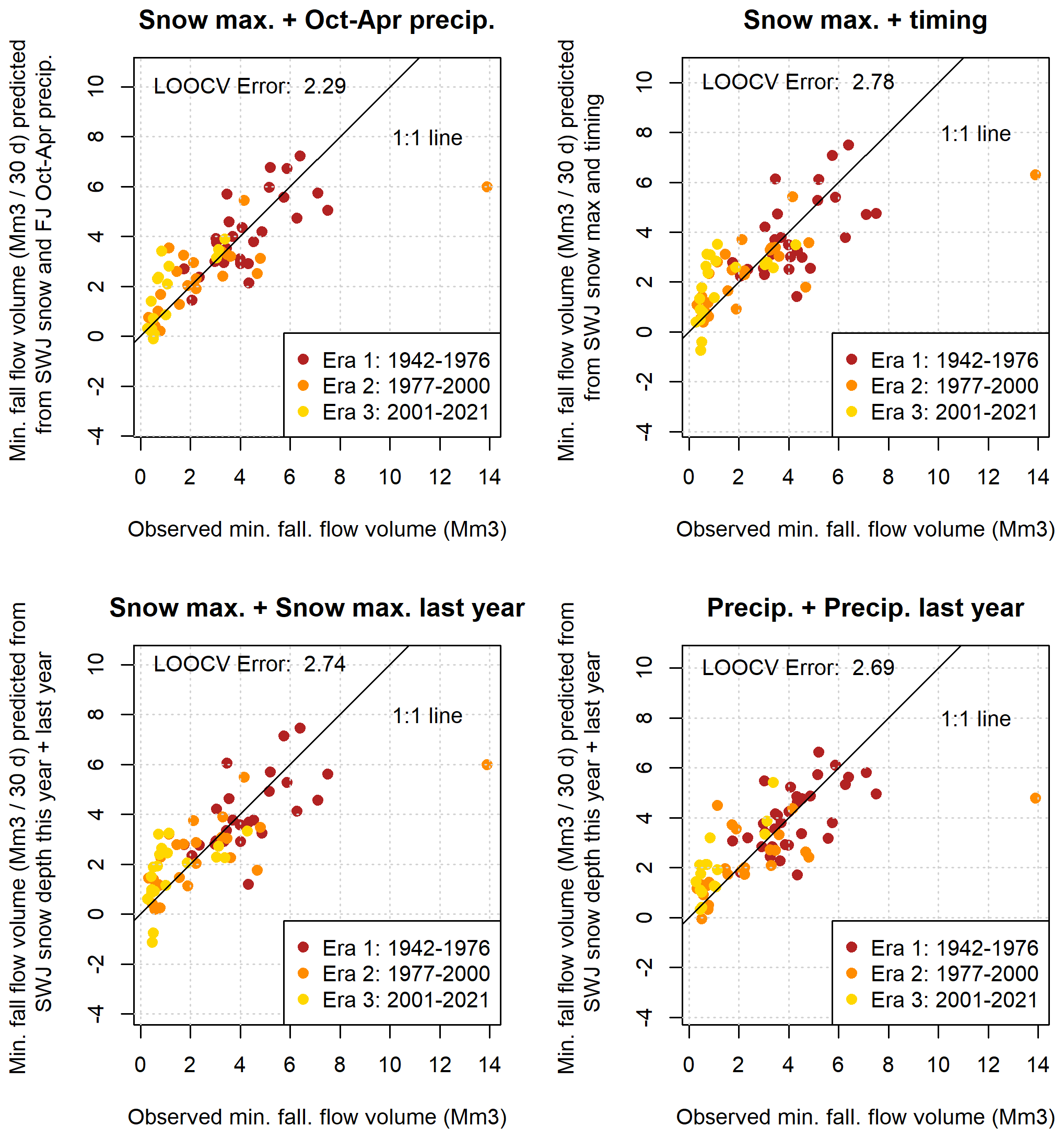
Table A5 Linear model diagnostics for two-predictor models of P_spill. Reference ET was not included in two- and three-predictor models due to an insufficient sample size. (See Table A1 for description of predictor IDs.)

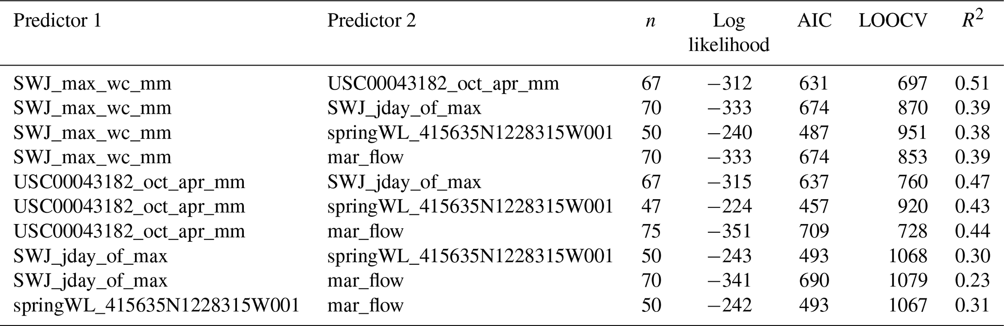
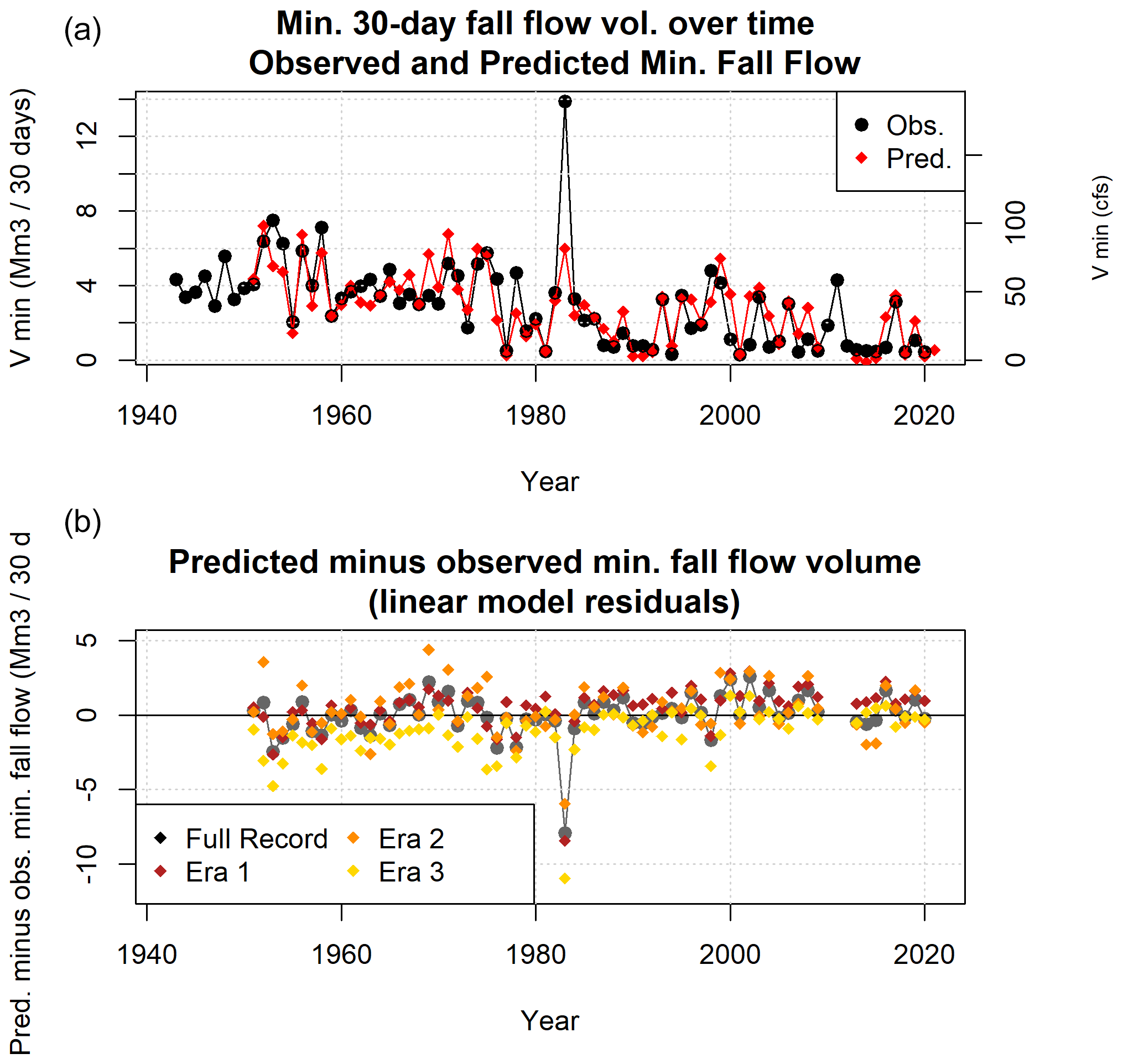
Figure A5 Observed and predicted minimum 30 d dry season baseflows both trend downward between the three eras of the period of record (a). The predicted-minus-observed difference (residual) over time also reflects this trend, underpredicting minimum flows pre-1977 and overpredicting them post-2000  (b). The predictive model is based on observations from the full record, but three additional models were generated based on only the observations from eras 1, 2, and 3. Residuals based on era-1 data are similar to those of the full record, era-2 residuals tend to overpredict more than the full record, and era-3 residuals show better performance post-2000, but significant underprediction pre-2000, than the full record.

Table A6 Linear model diagnostics for three-predictor models of P_spill. Reference ET was not included in two- and three-predictor models due to an insufficient sample size. (See Table A1 for description of predictor IDs.)

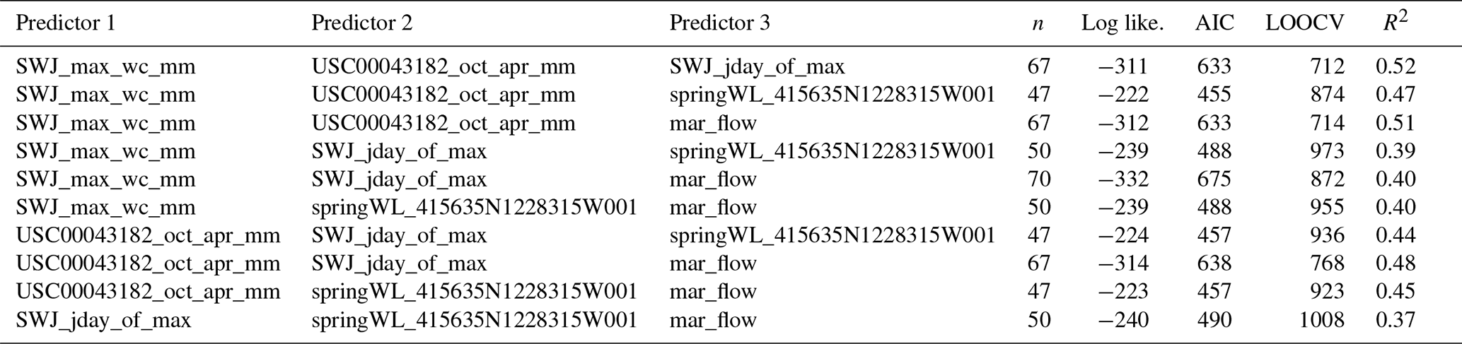
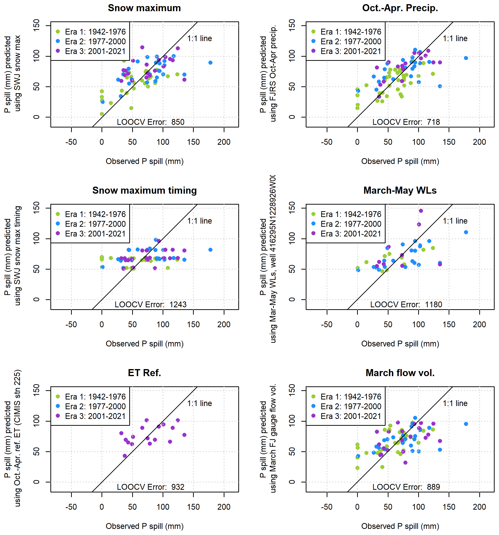
Figure A6 Single-predictor models of P_spill, the cumulative precipitation after the dry season needed to generate 120 cfs of flow in the Scott River.

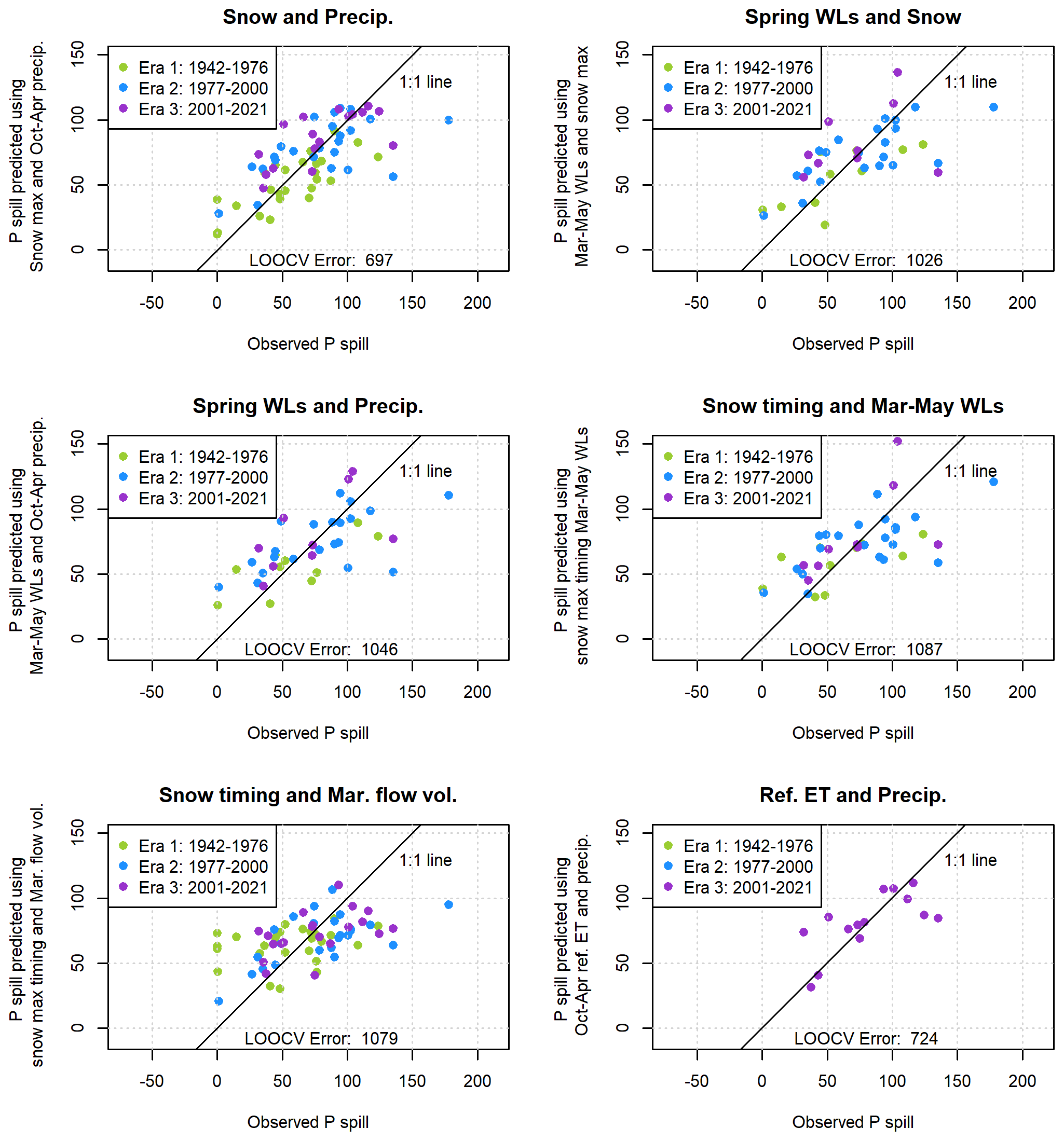
Figure A7 Two-predictor models of P_spill, the cumulative precipitation after the dry season needed to generate 120 cfs of flow in the Scott River.

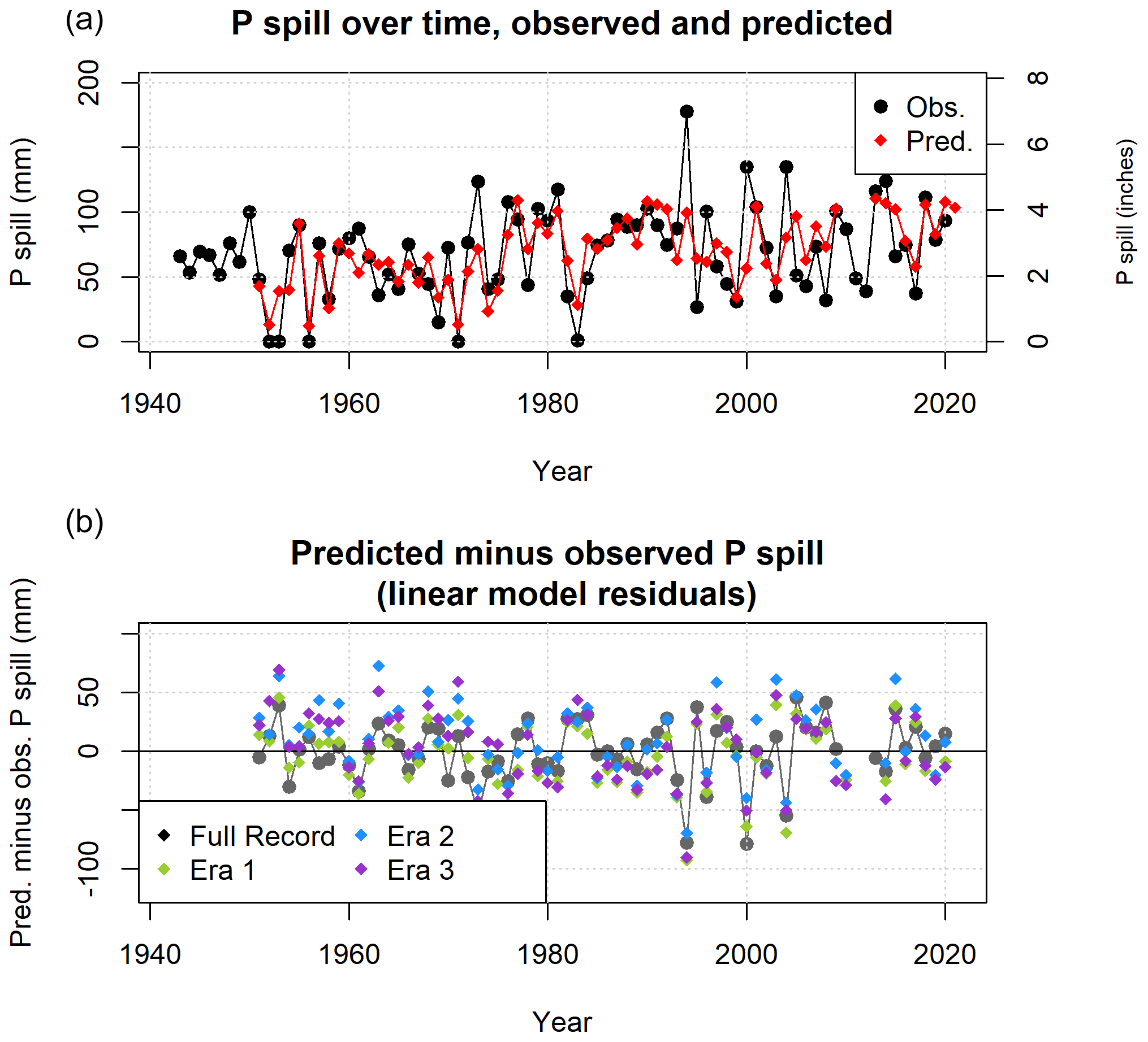
Figure A8 Observed and predicted values of P_spill (a) indicate a worse model fit for the P_spill prediction than for minimum 30 d dry season baseflows. Serious overprediction in era 1 is followed by more mixed over- and underprediction in eras 2 and 3 (b). The overall P_spill model is based on observations from the full record, but three additional models were generated based on only the observations from eras 1, 2, and 3. Residuals based on era-1 data are generally lower than those from eras 2 or 3, or from the full record.

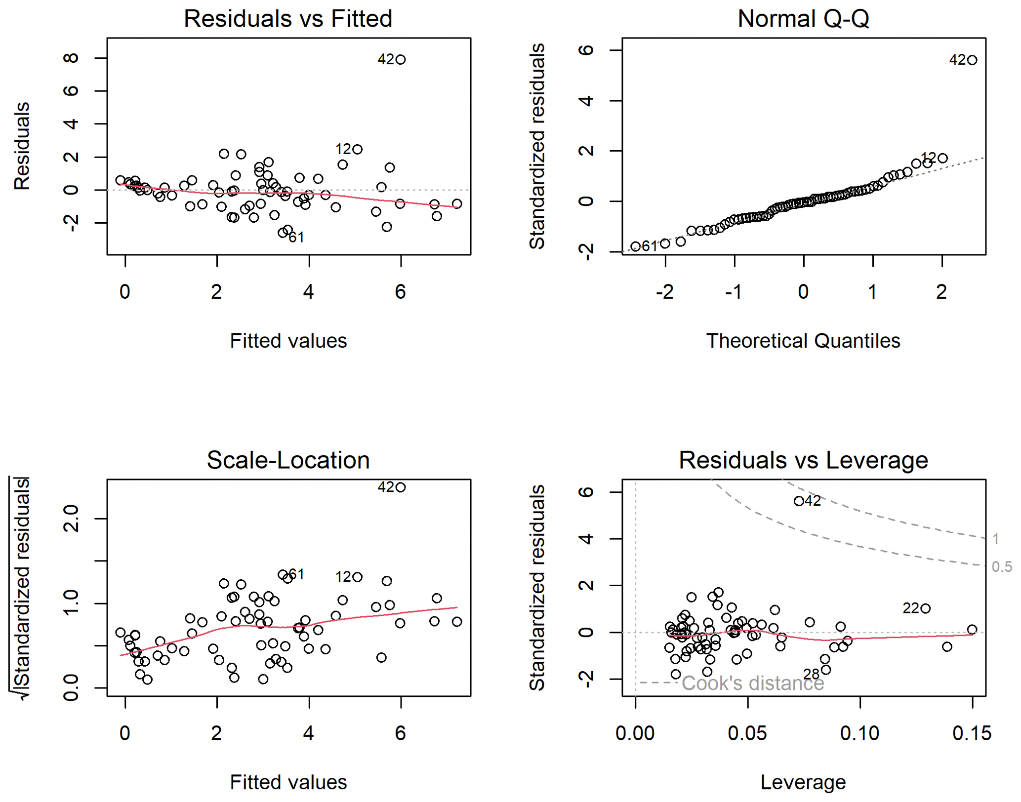
Figure A9 Diagnostic plots for the selected predictive models of V_min. See Sect. A5 for discussion of outliers.

Figure A10 Diagnostic plots for the selected predictive models of P_spill.