the Creative Commons Attribution 4.0 License.
the Creative Commons Attribution 4.0 License.
 | 13 Feb 2024
Extending the utility of space-borne snow water equivalent observations over vegetated areas with data assimilation
Melissa L. Wrzesien
Sujay V. Kumar
Eunsang Cho
Kristi R. Arsenault
Paul R. Houser
Carrie M. Vuyovich
Snow is a vital component of the earth system, yet no snow-focused satellite remote sensing platform currently exists. In this study, we investigate how synthetic observations of snow water equivalent (SWE) representative of a synthetic aperture radar remote sensing platform could improve spatiotemporal estimates of snowpack. We use a fraternal twin observing system simulation experiment, specifically investigating how much snow simulated using widely used models and forcing data could be improved by assimilating synthetic observations of SWE. We focus this study across a domain in the western USA and Canada, simulating snow at 250 m resolution and hourly time steps in water year 2019. We perform two data assimilation experiments, including (1) a simulation excluding synthetic observations in forests where canopies obstruct remote sensing retrievals and (2) a simulation inferring snow distribution in forested grid cells using synthetic observations from nearby canopy-free grid cells. Results found that, relative to a nature run, or assumed true simulation of snow evolution, assimilating synthetic SWE observations improved average SWE biases at maximum snowpack timing in shrub, grass, crop, bare-ground, and wetland land cover types from 14 %, to within 1 %. However, forested grid cells contained a disproportionate amount of SWE volume. In forests, SWE mean absolute errors at the time of maximum snow volume were 111 mm and average SWE biases were on the order of 150 %. Here the data assimilation approach that estimated forest SWE using observations from the nearest canopy-free grid cells substantially improved these SWE biases (18 %) and the SWE mean absolute error (27 mm). Simulations employing data assimilation also improved estimates of the temporal evolution of both SWE and runoff, even in spring snowmelt periods when melting snow and high snow liquid water content prevented synthetic SWE retrievals. In fact, in the Upper Colorado River region, melt-season SWE biases were improved from 63 % to within 1 %, and the Nash–Sutcliffe efficiency of runoff improved from −2.59 to 0.22. These results demonstrate the value of data assimilation and a snow-focused globally relevant remote sensing platform for improving the characterization of SWE and associated water availability.
- Article
(6315 KB) - Full-text XML
-
Supplement
(1295 KB) - BibTeX
- EndNote


Snow plays important roles in the earth system by regulating global temperatures and cooling the land surface because of its reflective properties (Barry, 2002). Snow is also a major source of water storage for many regions, especially in areas that rely on snowpack to sustain water resources during the dry season. In fact, it has been estimated that more than 2 billion people around the world are reliant on seasonal snowmelt for their water supply (Barnett et al., 2005). Snowpack is the natural “integrator” of climatic conditions and offers more predictability of water availability than variables with shorter memory, such as precipitation and streamflow (Terzago et al., 2023). Accurate winter estimates of snowpack are therefore critical for water management and agricultural planning (Koster et al., 2010). For example, in the western USA, where a vast majority of streamflow originates from snow (Li et al., 2017), it is common practice to use the 1 April snowpack, the historical date of maximum snowpack in that region, for developing water supply estimates for later in the season. However, climate change impacts have led to increased variability in the snow seasonality (Livneh and Badger, 2020), with warmer temperatures reducing the amount of snow accumulation and seasonal snow storage, and advancing the timing of the spring melt. Therefore, accurate characterization of winter snowpack and its variability is critically important for making informed water supply quantifications.
In recognition of the critical need to have spatially distributed measurements of snow mass, there have been several efforts to measure and estimate SWE from many different remote sensing platforms in the past several decades. Airborne lidar systems have been able to provide high resolution, accurate measurements of snow mass (Painter et al., 2016), but this approach has significant logistical barriers for global and frequent snow measurements, and the hydrologic utility of a practical spaceborne lidar platform is limited (Kwon et al., 2021). In the past three decades, snow depth and SWE estimates have been derived from passive microwave remote sensing measurements, but these measurements are at coarse spatial resolutions and have limited accuracies over deep and wet snow, complex terrain, and dense vegetation (Derksen et al., 2014; Foster et al., 2005). Active microwave remote sensing instruments, such as synthetic aperture radars (SARs), can provide finer spatial resolution measurements to help resolve some of these issues. For example, C-band SAR observations from the Sentinel-1 constellation have shown promise in obtaining high quality, moderate resolution (1 km) observations in deep snow environments (Lievens et al., 2019). A volume scattering radar approach, using X- and Ku-band SAR, has also been demonstrated in several airborne campaigns and proposed for multiple snow mission concepts (Yueh et al., 2009; Rott et al., 2010) because of its potential to achieve high resolution and global coverage over a range of snow depths. While these microwave instruments can observe in nighttime and cloudy conditions, they are still limited over areas with dense vegetation (Tsang et al., 2022). Furthermore, all spaceborne instruments have inherent coverage gaps due to their orbital and revisit configurations.
To overcome these limitations, modeling and data assimilation systems are needed that can extend the coverage and utility of available measurements to areas, times, and variables that are not directly observed. In this article, we present a novel approach through data assimilation, designed specifically to improve the usefulness of spaceborne SWE retrievals over forested areas. The approach is demonstrated using an observing system simulation experiment (OSSE; e.g., Cho et al., 2023; Errico et al., 2007) which is an approach used to formally assess the impact of the data to be collected from an anticipated mission. Several prior studies have examined the use of OSSEs for snow mission studies (Garnaud et al., 2019; Kwon et al., 2021; Wrzesien et al., 2022). Among them, SAR-focused OSSEs have been conducted by Garnaud et al. (2019) and Cho et al. (2023) to assess the utility of hypothetical snow observations. Garnaud et al. (2019) focused on a Ku-band SAR to quantify trade-offs between sensor configurations (e.g., various spatial resolutions and revisit frequencies) with retrieval algorithm accuracy and SWE performance in southern Quebec, Canada, where temperate forests are dominant with shallow and moderate snowpack conditions. Cho et al. (2023) conducted a X-/Ku-band SAR OSSE with an achievable sensor configuration (1 km spatial resolution, 7 d revisit frequency, and orbital configurations) focusing on mountainous environments in western Colorado and testing the degree to which various SAR retrieval capabilities in different forest densities and snow volumes could improve observationally based SWE estimates. Here we build on this prior research by developing an OSSE covering the entire western USA and portions of Canada. We simulate finer-scale (250 m) synthetic SWE observations that could be provided from a future X-/Ku-band SAR mission, which are then incorporated within a land surface model (LSM) through data assimilation to assess their capability to improve snow state estimates and the integrated impact on hydrologic states in space and time. The assimilation experiments here are conducted with and without a novel strategy to extend SAR-based SWE estimates from unforested regions into forested landscapes where SAR retrievals of the snowpack may be obscured by the forest canopy.
The primary contribution of this paper is the development of a viable strategy for extending hypothetical remotely sensed SWE retrievals from a volume-scattering X-/Ku-band SAR satellite mission into difficult-to-observe forest landscapes. We specifically focus on addressing the following questions:
-
What is the added utility of spaceborne active remote sensing SWE retrievals (assuming retrievals meet currently defined mission requirements) across the Western USA and Canada?
-
How much can spatiotemporal representations of SWE be improved by focusing on developing observationally based snow estimates over areas with dense vegetation, where SAR sensors may be limited?
-
How much added hydrologic utility can be obtained through spaceborne active remote sensing measurements and data assimilation approaches, particularly when coverage over forested areas is improved?
Section 2 describes the study domain and OSSE modeling setup. This is followed by a description of the results (Sect. 3), a discussion of the findings (Sect. 4), and the study's conclusions (Sect. 5).
2.1 Study domain and OSSE setup
An OSSE is used to assess the value of the data to be collected from an anticipated mission. OSSEs often consist of the following steps: (1) developing a “nature run” that uses a state-of-the-art model employed with the best available boundary conditions (Sect. 2.1); (2) using the nature run to generate simulated remote sensing observations, accounting for sources of sensing limitations, sensing uncertainties, and orbital configurations (Sect. 2.2); (3) incorporating the simulated observations (often through data assimilation, Sect. 2.3) in a separate, “open loop” model configuration with accuracies representative of common modeling biases and uncertainties; and (4) evaluating how much the simulated remote sensing data improve the open loop model performance relative to the nature run. In addition to this OSSE approach, this study goes further by (1) testing the degree of improvement to both the remotely sensed variable (i.e., SWE) and the resulting changes to land surface runoff in snow covered regions, and (2) developing two separate data assimilation experiments, one which masks simulated observations in forested pixels where SAR retrievals may be most challenging and the other including a novel approach for inferring SWE in forested pixels using simulated observations from nearby, unforested pixels (Sect. 2.4). The details of the OSSE setup used in this study are described in more depth throughout this section.
We employ the NASA Land Information System (LIS; Kumar et al., 2006), an infrastructure for high performance, ensemble-based land surface modeling and data assimilation to enable this OSSE. LIS encompasses several advanced land surface models that can simulate terrestrial water, energy, and carbon balances as well as related states such as soil moisture, land surface temperature, and SWE, among others. These include different versions of community models such as Noah (Ek et al., 2003), Variable Infiltration Capacity (VIC; Liang et al., 1994), Catchment (Koster et al., 2000), Joint UK Land Environment Simulator (JULES; Best et al., 2011), and Noah-MP (Niu et al., 2011). The LIS framework also includes support for specialized models that are designed to provide more detailed representations of certain land surface processes (e.g., snow) while enabling interaction with LSMs that solve for water, energy, and carbon balances at a macroscale. For example, the advanced snow physics model called SnowModel (Liston and Elder, 2006) has been incorporated within LIS in a manner that allows coupling to existing LSMs. This structure allows the use of the advanced snow physics from SnowModel while leveraging the existing process schemes (e.g., sub-surface, groundwater, and canopy) within the LSMs. Here we utilize these unique capabilities for enabling the OSSE integrations. The study is conducted over a large domain (Fig. 1) covering the western USA and southern Canada from 31 to 55∘ N and 93 to 130∘ W at a 250 m spatial resolution. As shown in Fig. 1, this modeling domain encompasses a broad range of vegetation types, topographical regimes, and water resources regions of the Pacific Northwest, California, Great Basin, and Upper Colorado. 22 % of the domain is covered by forests, with grasslands, croplands, and shrublands accounting for 20 %, 23 %, and 26 % of the domain, respectively. Forests dominate the coverage of areas with significant snowpack, occupying 58 % of regions that are in the mid-elevation range of 2500–3500 m and 15 % of the areas with elevations over 3500 m. From a modeling perspective, the domain extent of Fig. 1 (∼83 million land grid points) is computationally challenging. The scalable high performance computational and parallel inputting and outputting capabilities of NASA LIS were leveraged to enable these simulations. A multiprocessor configuration involving approximately 1000 processors was employed to facilitate large model simulations for the nature run, open loop simulation, and two simulations with data assimilation.
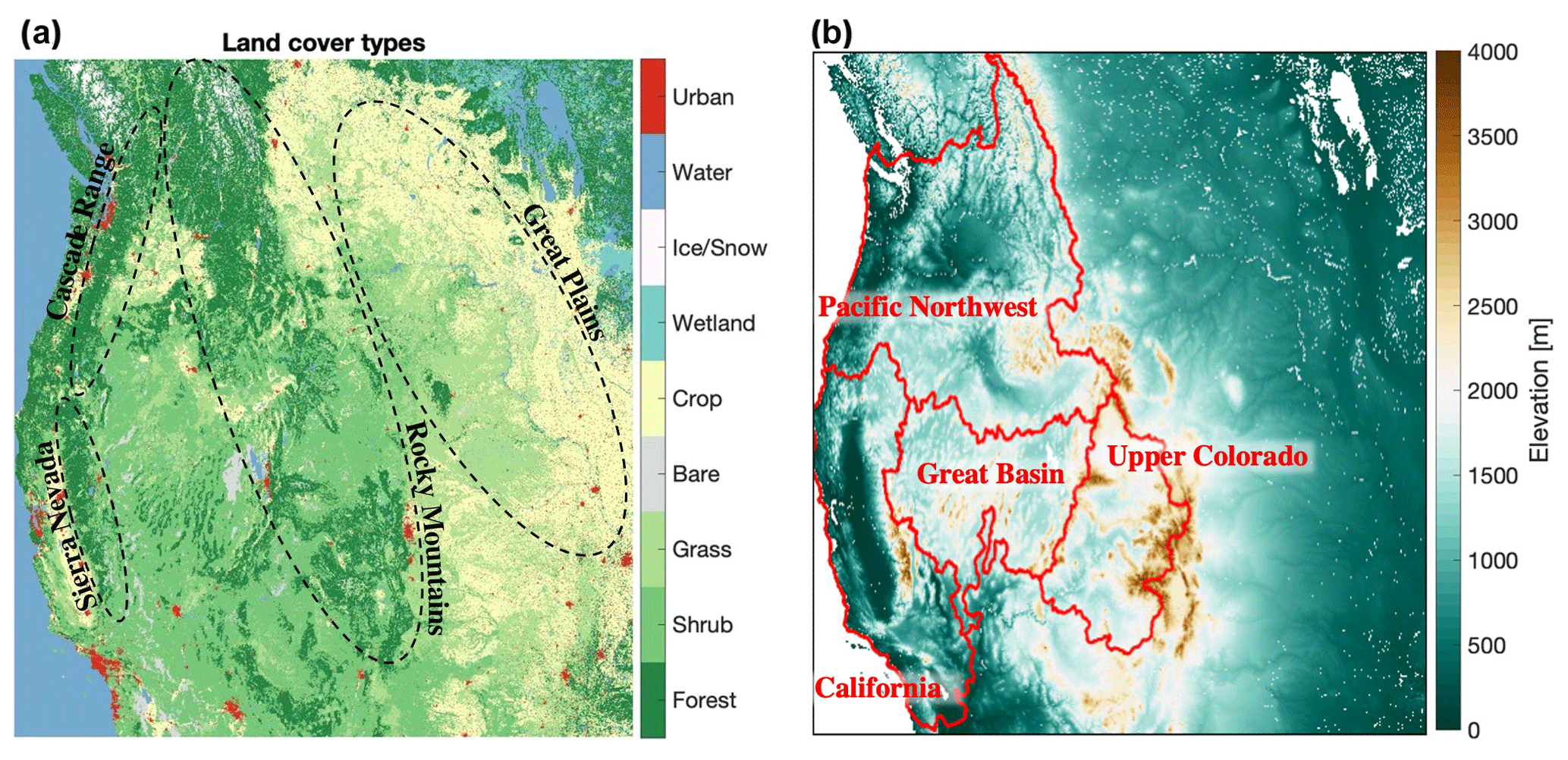
Figure 1Maps of the land and vegetation classes (a) and elevation (in meters) (b) used in the simulations. Outlines and labels in panel (a) indicate regions discussed in the Results (Sect. 4). Red contours in panel (b) indicate hydrologic regions used in the analysis.
Simulations in this study are conducted by forcing LIS LSMs with the surface meteorology from NASA's Modern Era Retrospective Reanalysis, version 2 (MERRA-2; Gelaro et al., 2017) and ECMWF Reanalysis, version 5 (ERA5; Hersbach et al., 2020) products. The model integrations were conducted for the water year 2019 (September 2018–September 2019), which was a wetter than normal year based on the long-term average meteorological conditions over this domain.
The open loop and data assimilation integrations performed in this study are conducted using the Noah land surface model with multi-parameterization (Noah-MP) version 4.0.1 (Niu et al., 2011) and forcing from ERA5. The Noah-MP model evolved from the Noah LSM, with multiple options for various land surface processes. It represents energy, water, and carbon balances at the land surface by accounting for processes related to infiltration, evaporation, transpiration, runoff generation, and groundwater recharge. A TOPMODEL-based runoff model (Beven et al., 2021) is used to calculate surface runoff and groundwater discharge. Options for prognostic vegetation dynamics models that represent the growth and senescence of vegetation are also available within Noah-MP. A two-stream radiative transfer approach is employed to calculate surface energy processes. Finally, a multilayer snowpack model (with up to three layers) is used to account for snowmelt metamorphisms, compaction by overlying snow, sublimation of canopy intercepted snow, and snowmelt–refreeze cycles within Noah-MP (Niu and Yang, 2004).
Snow states like snow depth and SWE were also modeled across the western USA (domain highlighted in Fig. 1) at 250 m resolution and hourly time steps using a state-of-the-art and physically based single-layer snow model (named SnowModel; Liston and Elder, 2006), provided forcing from MERRA-2 with LIS-provided lapse rates and topography-based meteorological downscaling approaches, like incoming shortwave corrections based on topographical shading (Cosgrove et al., 2003; Kumar et al., 2013). SnowModel has seen widespread use in the snow community, demonstrating the capability to resolve snow evolution in a variety of landscapes and complex snow processes like the redistribution of snow via wind, and the resulting impact on snow distribution, melt season snow duration, glacier mass balance, and snow habitat for species like polar bear and Dall sheep (Hiemstra et al., 2002; Liston et al., 2016; Mahoney et al., 2018; Mernild et al., 2017; Sturm and Wagner, 2010). In addition to wind redistribution, snow evolution within SnowModel accounts for a wide variety of snow processes, including snow sublimation, snow grain size evolution, solar topographical shading, canopy shading, and canopy snow interception. Through the coupling within LIS, Noah-MP snow states and the resulting snow-driven runoff were updated using the SnowModel outputs at hourly time steps for each grid cell.
Preliminary research has shown that relative to Noah-MP, LIS simulations coupling Noah-MP with SnowModel have improved the volume and spatial distribution of simulated snow depth and SWE (Arsenault et al., 2021; Wrzesien et al., 2022). Therefore, the coupled SnowModel and Noah-MP model was a prime candidate for the “nature run” in this study, or the simulation (1) most representative of the true underlying spatiotemporal snow states from which simulated observations were derived (Sect. 2.2), and (2) the simulation the assimilated model was compared against. Here the nature run and open loop simulations detailed above were compared with a widely used western USA snow reanalysis product (Fang et al., 2022) to ensure that (1) the nature run exhibited reasonable model accuracy and (2) the departure between the open loop simulation and nature run are representative of common regional, continental, and global modeling efforts (Figs. S1 and S2 in the Supplement). The OSSE developed for this study is a “fraternal twin” OSSE wherein two different models are used to simulate snow in the open loop (Noah-MP) and nature run (SnowModel) simulations. This approach is selected since “identical twin” OSSEs, which use the same model, can result in less divergence in model states and information content, biasing the degree of model improvement that could come from assimilating an observation (e.g., Yu et al., 2019). More information on the difference between the open loop and nature run models can be found in Table S1 in the Supplement.
2.2 Observation simulator
Synthetic SWE retrievals at 250 m spatial resolution, representative of a hypothetical X- and Ku-band SAR mission, are simulated from the nature run. To do this, the orbital swaths are simulated using TAT-C (Le Moigne et al., 2017). TAT-C is a NASA software system designed for future distribution spacecraft missions that enables us to explore a range of feasible design options (e.g., constellation vs. single, geostationary vs. polar-orbiting, low vs. high temporal frequencies) to estimate optimal gains for the given mission configuration. Previous OSSEs have been conducted to test the impact from different snow mission configurations (e.g., Garnaud et al., 2019). Here we instead focus on demonstrating the value of a gap-filling approach (Sect. 2.4) for estimating snow in forested landscapes where SAR retrievals may be most challenging. Therefore, we used TAT-C to design a conservative mission configuration consisting of a small constellation of X- and Ku-band SAR satellites. Using a 10–14 d revisit frequency, depending on latitude, TAT-C orbital swaths were applied to the nature run outputs to simulate the satellite viewing area. The remote sensing spatial coverage is simulated by extending the ground track to a swath width. The daily viewing extents are then simulated as a daily binary map (so-called cookie cutter) masking the surface as viewed or not at a 250 m spatial resolution.
Based on an error level of 20 %, spatially and temporally uncorrelated random errors drawn from a Gaussian distribution are added to the synthetic SWE retrievals. This 20 % error level is selected using a conservative estimate of SWE measurement uncertainty for a volume-scattering X-/Ku-band SAR mission based on developed mission design concepts and ground validation. For example, the ESA Cold Regions Hydrology High-Resolution Observatory (CoREH2O) mission expected to meet instrument and retrieval requirements of ±30 mm accuracies for an SWE of 300 mm and ±10 % for an SWE greater than 300 mm (Rott et al., 2010, 2012). Similarly, the Canadian Terrestrial Snow Mass Mission (TSMM) concept that is currently under development aims to achieve better than 20 % measurement uncertainty for an SWE greater than 50 mm, though it is expected to have higher uncertainties in deep snow conditions (e.g., ≥ 200 mm SWE) (Garnaud et al. 2019). Airborne and tower-based field data have demonstrated that a combination X- and Ku-band system can provide SWE retrievals over a range of snow conditions at accuracies better than 20 % (Zhu et al., 2018, 2021; Tsang et al., 2022; Durand et al., 2024; Singh et al., 2023). However, we use an assumption of uniform error levels throughout the domain, whereas in reality, the errors are likely to be dependent on other factors, including the terrain characteristics, snow characteristics, and vegetation. This is discussed more in Sect. 4.
2.3 Data assimilation setup
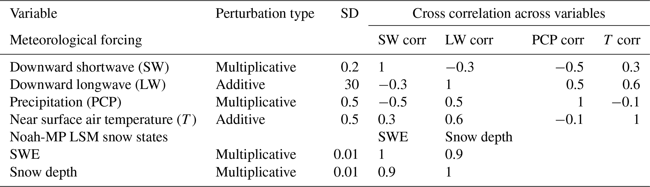
A one-dimensional ensemble Kalman filter (EnKF; Reichle et al., 2002) is used to assimilate the synthetic observations within the open loop configuration of the model. The EnKF is widely used for land data assimilation studies (Kumar et al., 2022), as it provides a flexible approach for the treatment of model and observation errors and non-linear models. An ensemble of model realizations is used by EnKF to assess and propagate model errors. In this instance, the ensemble requirement further adds to the significant computational requirements of the large model domain (Fig. 1) and fine spatial resolution of the simulations (250 m). Therefore, a five-member ensemble with perturbations applied to the meteorological variables and model prognostic fields are used for simulating uncertainty in the modeled estimates. Table 1 details the parameters for meteorological and model state perturbations, which are based on recent snow data assimilation studies (Lahmers et al., 2022; Kwon et al., 2021). Though a larger ensemble size is better for ensuring sufficient sampling density, our choice of five ensembles is reasonable given that the model state vector used in the assimilation consists of only two variables: the total SWE and snow depth. The assimilation setup employs a sequential update strategy, where at each time step an ensemble of model forecasts is propagated forward in time, followed by an update based on observational inputs. The model states are updated toward the observations based on the relative uncertainties in the model and observations using the following equation at a certain time k:
where xk and yk are the model and observation state vectors, respectively. The term Hk represents the observation operator that maps the model states to the observed variables. The superscripts i− and i+ represent the ith ensemble member before and after the update, respectively. Kk is the “Kalman gain” term, which allows the weighting of the observations and model forecasts to be a function of the model and observation error covariances.
Table 1Model forcing and state-variable perturbations used by the five-member ensemble of LIS simulations. SD references the standard deviation of the perturbation.
The data assimilation procedure detailed here assimilated the synthetic SWE retrievals (Sect. 2.2) with the open loop simulation. The degree to which the simulation with data assimilation approached SWE simulated by the nature run is intended to represent the extent to which an SAR remote sensing platform with the SWE retrieval characteristics from Sect. 2.2 could be combined with a land surface model to provide near-real-time estimates of SWE at 250 m resolution. However, the SAR observations synthesized in this study have known issues with observing snow with high liquid water content and dense forest cover. Therefore, synthetic observations at each time step were masked at grid cells where the most dominant land cover type from the North American Land Change Monitoring System (NALCMS; Latifovic et al., 2017) was forested, including deciduous, evergreen, and mixed forest cover (Fig. 1). Synthetic observations were also masked at grid cells where and when snow was experiencing melt, identified by the presence of liquid water in the snowpack from the nature run. Although limited in area, grid cells with “ice” land cover (Fig. 1) were also excluded. In this study, this simulation which used assimilation only in unforested, non-melting, and ice-free grid cells is termed “data assimilation, without the forest strategy” (DA). In Sect. 2.4 below, we present a novel approach used to infer SWE in grid cells with forests using the nearest canopy-free synthetic observations.
2.4 Extending observations over forests
The 1-D EnKF approach employed here updated each model grid SWE from the open loop simulation based on the observations available at that grid point. Though studies have employed 3-D EnKF approaches to spatially propagate observational information to neighboring grid cells (De Lannoy et al., 2012), here we relied on 1-D updates due to several factors. First, a 2-D update requires the knowledge of spatial error correlations and their variability, which is challenging to specify (Ying, 2020). Most prior studies using such schemes employ uniform specifications and are limited to small domains. Second, a 2-D update increases the size of the state vector and consequently requires the use of a larger ensemble. This, combined with the added computational expense of a 2-D analysis, significantly increases the computational cost. Therefore, we employed an alternate approach that is computationally more efficient while allowing the extension of observations to nearby areas.
Assuming that the SWE retrievals from the hypothetical SAR instrument are limited over areas where the dominant vegetation type are forests (Fig. 1a), we employ a novel approach to extend the observations obtained in non-forested areas (Fig. 2). For every forested location, valid retrievals over nearby non-forested locations within a radius of influence of 750 m are identified. An observation at the forested pixel is then estimated by scaling the model SWE by the ratio of the average observed SWE to a modeled SWE over the “clearing” areas (Fig. 2). This scaled observation is then used for assimilation over the forested pixel. Here we implicitly use the spatial correlations inherent in the model between forested and clearing areas to extend observational coverage over the clearing to forested locations, the aforementioned “data assimilation, with the forest strategy” (symbolized by DA+F in Sect. 3). To evaluate the accuracy and added value of this scaling approach, we compare SWE and runoff from the nature run simulation, versus simulations with data assimilation both (1) employing the forest scaling strategy discussed here and (2) masking synthetic observations in forested grid cells (Sect. 2.3).
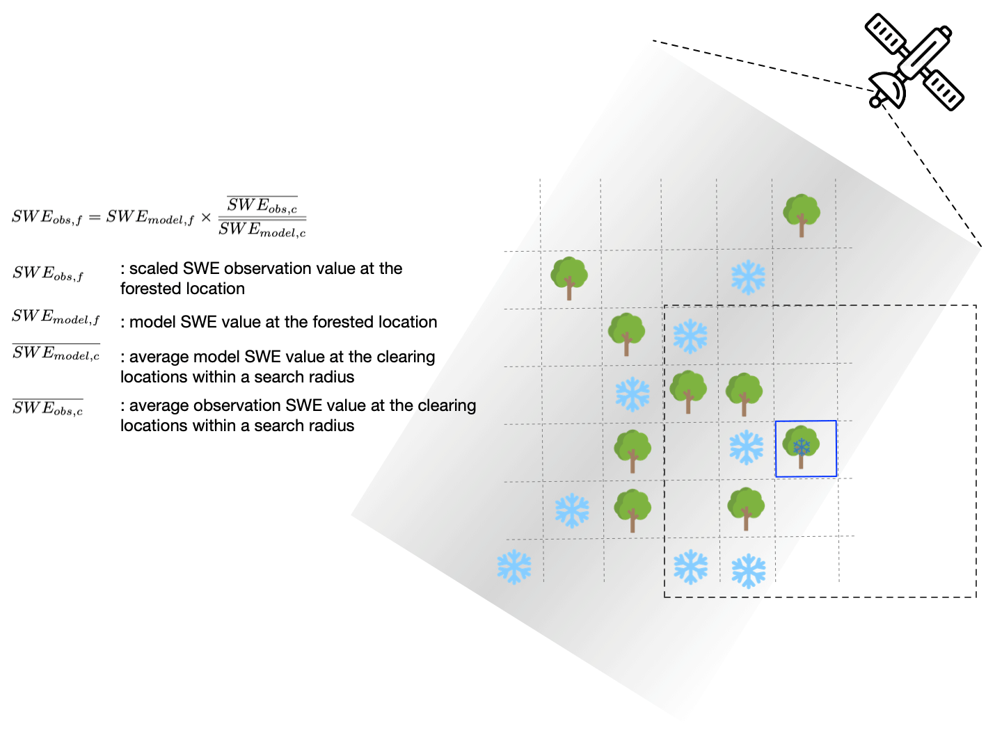
Figure 2Conceptual depiction and equations demonstrating the forest strategy used here, which estimates a SWE observation at a given grid cell (outlined blue box) based on the modeled SWE (SWEmodel,f) and the ratio between the average synthetic SWE observations () and average modeled SWE () from grid cells within a 750 m radius (dashed box). The light gray shading represents the satellite swath, the tree icons indicate forested locations, and the snowflake icons represent grid cells with valid SWE retrievals at non-forested locations. The grid cell from this example is near the satellite swath edge, so observations are unavailable in the nearby regions south and east of this pixel.
In this section, we compute the difference between the open loop simulation, nature run, and the two open loop simulations with data assimilation: one masking synthetic observations over regions with forests, and time periods with melting snow, and ice; and the other applying the same data assimilation but extending snow estimates in forested regions using the strategy from Sect. 2.4 and Fig. 2. The differences between these simulations are detailed in Sect. 2 and Table S1. We focus on the differences between these four simulations using (1) average SWE from the winter snow accumulation season, i.e., December, January, and February (DJF), when snowmelt is minimized and synthetic observations are masked by grid cells with liquid water content to the smallest degree; (2) spatially distributed SWE on 13 March, the date corresponding to the timing of maximum SWE volume in water year 2019; and (3) daily average SWE and total runoff for each day in water year 2019 over a number of selected hydrologic regions including the Pacific Northwest, California, Great Basin, and Upper Colorado (Fig. 1b).
The open loop and nature run simulations exhibited differences in both the volume and spatial distribution of average winter (i.e., DJF) SWE (Fig. 3a and b). Relative to the nature run, the open loop simulation tended to simulate lower elevation winter SWE that was both larger in magnitude and persisted for longer before melting. In the Pacific Northwest domain (Fig. 4), DJF average snow cover (defined as grid cells with mean DJF SWE exceeding 5 mm), was approximately 12 % larger for the open loop simulation than the nature run (Table 2). These snow extent biases were also apparent in the other hydrologic regions (Figs. S3–S5), where open loop snow extents exceeded snow extents from the nature run by 26 % in the Upper Colorado, 45 % in the Great Basin, and 6 % in California. Visually, the nature run had significant increases in the spatial variability of winter SWE, better representing the differences in SWE between mountain peaks and valleys, and the patchiness of snow cover in regions with winter snowmelt and ephemeral snow cover (e.g., Figs. 4, S1). Relative to the nature run, DJF SWE from the open loop simulation was biased high across the full modeling region (Fig. 3) by approximately 26 %, on average, with a mean absolute error of 41 mm and spatial coefficient of correlation of approximately 0.74. Across the Pacific Northwest (Fig. 4), DJF mean SWE biases were approximately 37 %, with a mean absolute error of 55 mm. Open loop model performance for the other hydrologic regions can be found in Table 2.
Table 2Simulation performance, relative to the nature run simulation, for the open loop (OL) simulation and the simulations with data assimilation, both with (DA+F) and without (DA) the forest strategy. Statistics are presented for the full domain, the four hydrologic regions, and all forested and unforested grid cells.
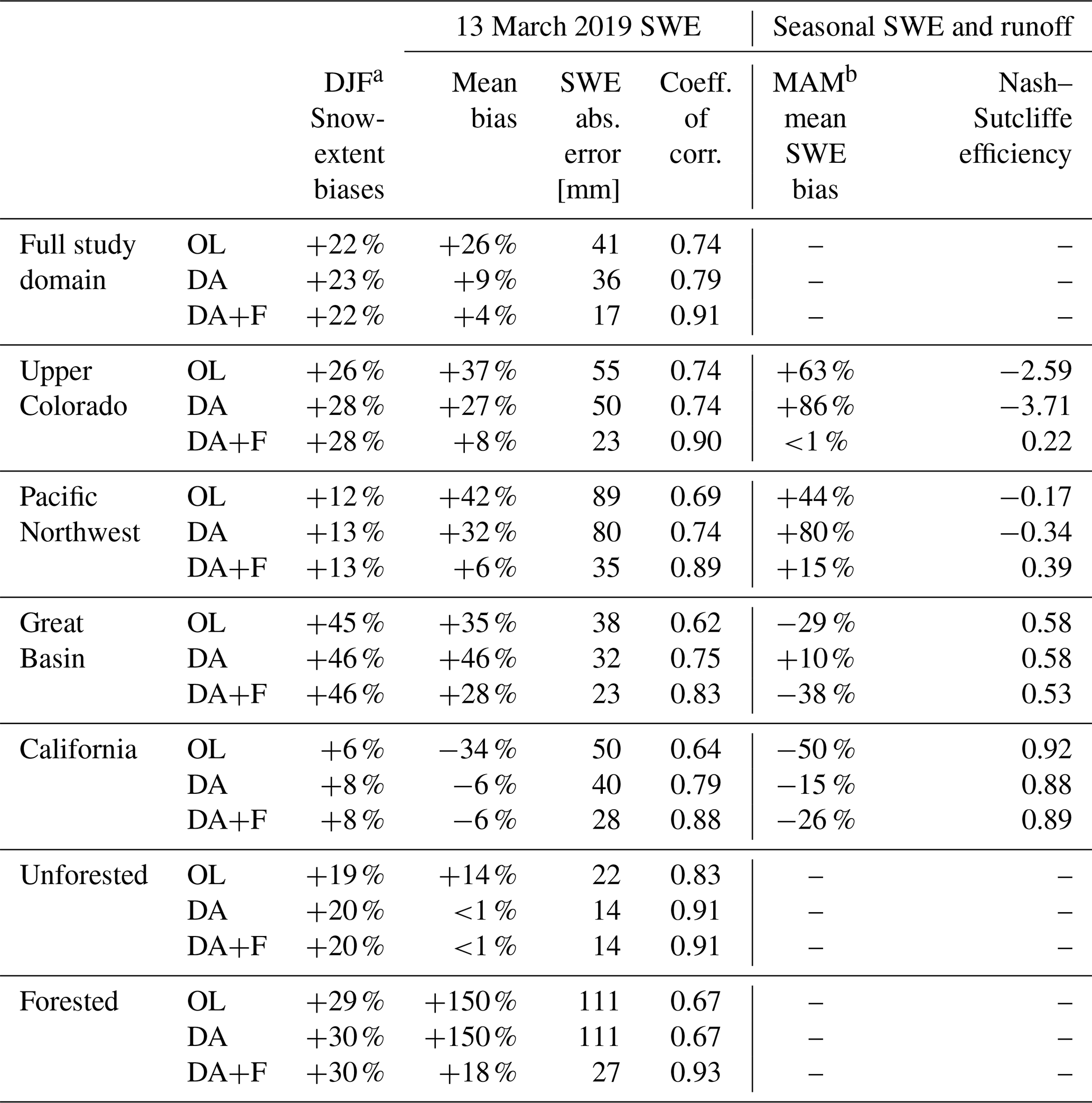
a DJF = December, January, and February. b MAM = March, April, and May (averages).
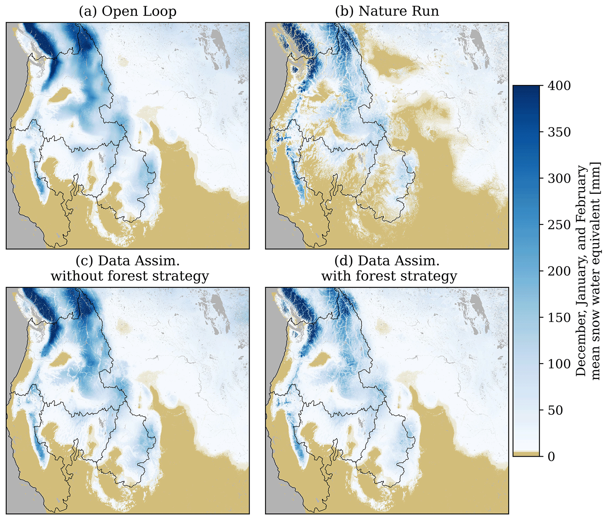
Figure 3Winter (December, January, and February) mean SWE simulated at 250 m resolution from the open loop (a) and nature run (b), and data assimilation simulations, both without (c) and with (d) the forest strategy presented in Sect. 2.4.
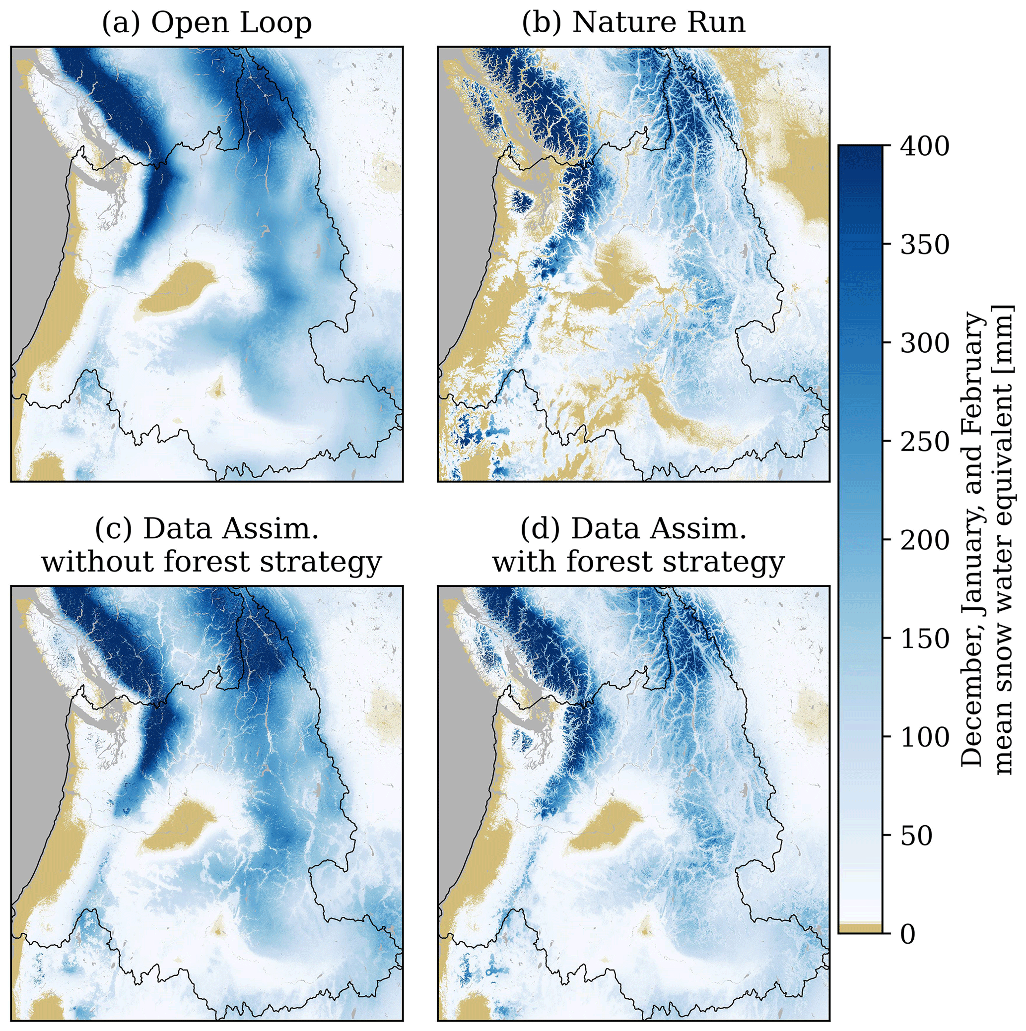
Figure 4Winter (December, January, and February) mean SWE in the Pacific Northwest region simulated at 250 m resolution from the open loop (a) and nature run (b), and data assimilation simulations, both without (c) and with (d) the forest strategy.
As expected, the simulations assimilating the synthetic SWE observations agreed with the nature run better than the open loop simulation. However, on 13 March 2019 (the date of maximum domain SWE volume), the simulation with data assimilation without the forest strategy had high-biased SWE across large portions of the Rocky Mountains and the Cascade Mountain range (Figs. 1 and 5b, e). Low-biased SWE was more common in the northernmost Canadian portions of the Rocky Mountains and Cascade Range, the western-montane regions in Washington state, the northern portions of the Great Basin, and the lower-lying elevations of the California Sierra Nevada. Additionally, despite the assimilation, snow extents were still biased high relative to the nature run (Fig. 3) at magnitudes similar to those of the open loop simulation (Table 2). This was driven by the expansive snow extents of the open loop simulation, which were decreased by data assimilation, but still resulted in widespread early-season SWE increases for short periods of time between synthetic observations (at 10–14 d frequencies), increasing to the number of grid cells with DJF SWE exceeding 5 mm (the threshold used to define average winter snow extents in Fig. 3).
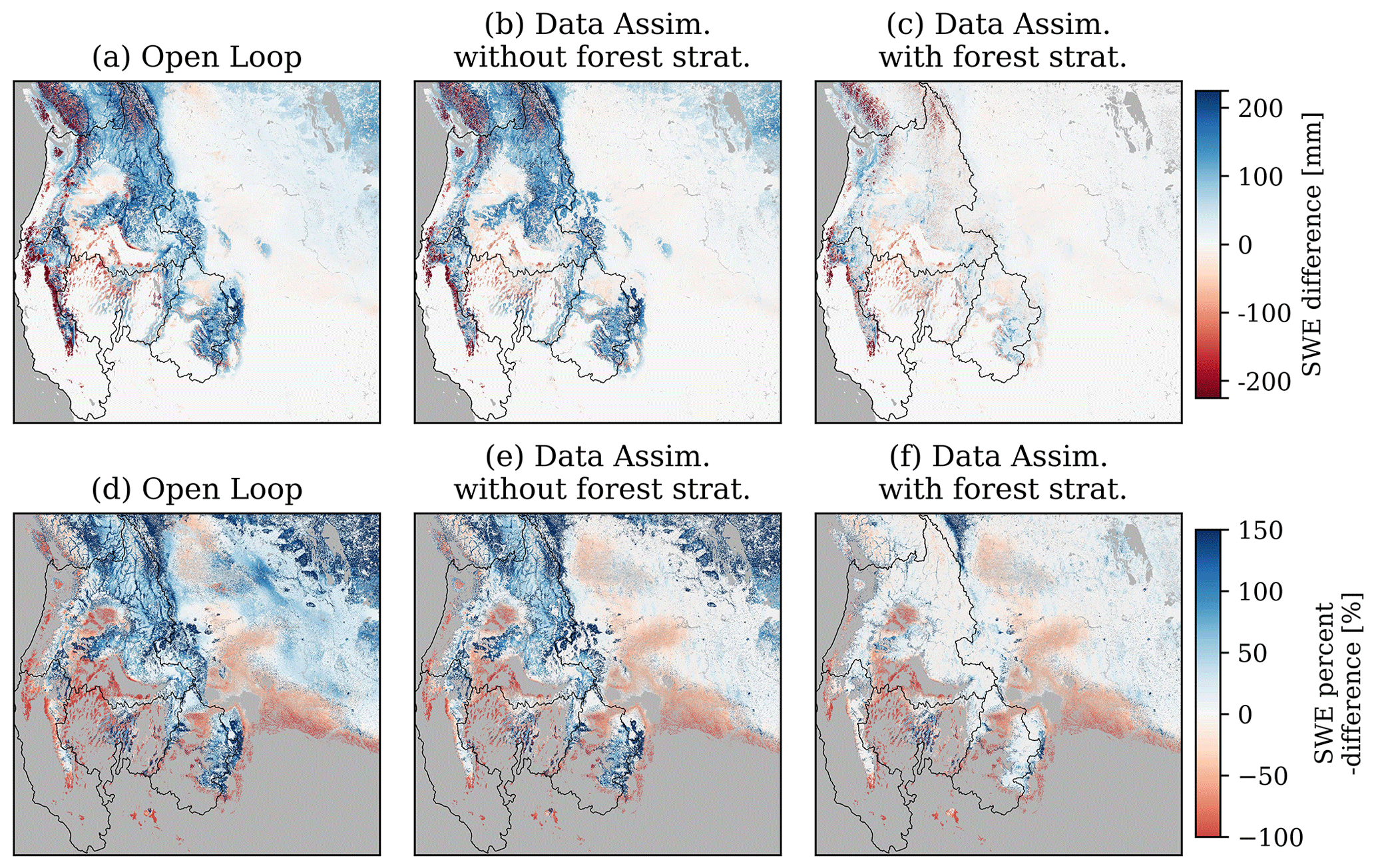
Figure 5The 13 March 2019 SWE difference (a–c) and percent difference (d–f), relative to the nature run, for the open loop simulation (a, d) and simulations with data assimilation, both with (c, f) and without (b, e) the forest strategy. The SWE percent-different maps (d–f) only compare grid cells where the SWE from the nature run was greater than 5 mm.
Assimilating the synthetic SAR observations without the forest strategy best improved SWE in shrub, grass, crop, bare, and wetland land cover types (Fig. 6b and c). For example, relative to the open loop simulation (Fig. 5a and d), data assimilation without the forest strategy (Fig. 5b and e) corrected the high SWE biases in the Great Plains (Fig. 1). While 13 March SWE in shrub, grass, crop, bare-ground, and wetland regions was typically small in magnitude, these land cover types accounted for 77 % of the modeling domain area, and 61 % of the domain total SWE volume on 13 March (Fig. 6a). In these regions, SWE from the open loop simulation had a mean absolute error of 22 mm, and a mean bias of approximately 14 %, relative to the nature run (Table 2). Data assimilation significantly improved the SWE bias in these land cover types to within 1 %, on average (Fig. 6b), with a mean absolute error of 14 mm, relative to the nature run.

Figure 6The SWE volume on 13 March 2019 broken down by land cover type in (a). For each land cover type, the interquartile range and median of SWE differences (b) and SWE percent differences (c) are calculated for the open loop simulation (black bars) and each simulation with data assimilation (blue bars). The SWE differences (b) and (c) are calculated relative to the nature run.
The data assimilation results discussed above did not use the synthetic observations over forested grid cells, where retrievals from SAR instruments may be either partially or fully occluded by the canopy overstory (Tsang et al., 2022; Ruiz et al., 2022; Huang et al., 2019). However, a significant portion of the snow volume in mid-latitude domains overlaps with forests. For example, although forests only covered approximately 22 % of the study region investigated here (Fig. 1a), forested grid cells contained just over 34 % of the total 13 March SWE volume, a volume about 10 % higher than the snow volume contained in the next-largest land cover type (Fig. 6a). In forested grid cells, SWE values simulated by the open loop simulation were biased high by approximately 87 mm (+150 %) on average (Fig. 6), with a mean absolute error of 111 mm (Table 2). These errors were propagated into the simulation with data assimilation without the forest strategy. Fortunately, the ratio between modeled SWE and synthetic SWE observations in forested grid cells and the nearest canopy-free grid cells had high levels of similarity. Therefore, estimating snow in forest regions using the nearest canopy-free pixels (Fig. 2) improved snow simulations significantly (Figs. 3d, 4d, and 5c, f). In fact, snow simulated in forest landscapes using data assimilation with the forest strategy agreed well with the nature run, exhibiting a 13 March SWE average bias in forested grid cells of only 14 mm (+8 %) (Fig. 6), and a mean absolute error of 27 mm. This forest strategy resulted in large-scale improvements to total domain SWE (Fig. 5), reducing the 13 March full-domain SWE volume bias by 28 %, and improving the spatial coefficient of correlation by 0.12, relative to the data assimilation simulation without the forest strategy.
The comparisons above focused on mean DJF SWE and SWE from the date nearest maximum snow volume (13 March 2019). However, assimilating the synthetic SWE data also improved estimates of snow water resources throughout the duration of the water year, even in periods when most snow covered regions were experiencing snowmelt and synthetic observations were masked. For example, in the Upper Colorado, approximately 75 % of the region had DJF snow cover with little or no winter snowmelt (Fig. 7). The simulation with data assimilation and the forest strategy substantially improved mean SWE evolution in the snow accumulation season in this hydrologic region (October–March in Fig. 7). However, snowmelt onset in the March, April, and May (MAM) months increased the number of grid cells experiencing snowmelt from the open loop model outputs, reducing the number of grid cells across the full Upper Colorado that could be observed by the synthetic SAR observations to approximately 5 %, on average, over this period of time. Despite this, since the simulation with data assimilation improved the volume, timing, and spatial distribution of maximum SWE, mean SWE evolution tracked the nature run simulation significantly better than the open loop simulation in the spring snowmelt period. In fact, relative to the nature run, MAM SWE from the open loop simulations was biased high by approximately 63 %, on average, in the Upper Colorado (Table 2). The simulation with data assimilation using the forest strategy improved this bias to less than 1 %, on average, over the same period. In this study, simulations using Noah-MP (open loop and data assimilation simulations) melted snow more rapidly in the latter half of the spring snowmelt season than the nature run simulation which evolved SWE using SnowModel (Sect. 2.1). Therefore, although maximum SWE volume, maximum SWE timing, and MAM SWE were improved by data assimilation, the timing of snow disappearance for the simulation with data assimilation using the forest strategy was approximately 18 d earlier than that of the nature run in the Upper Colorado.
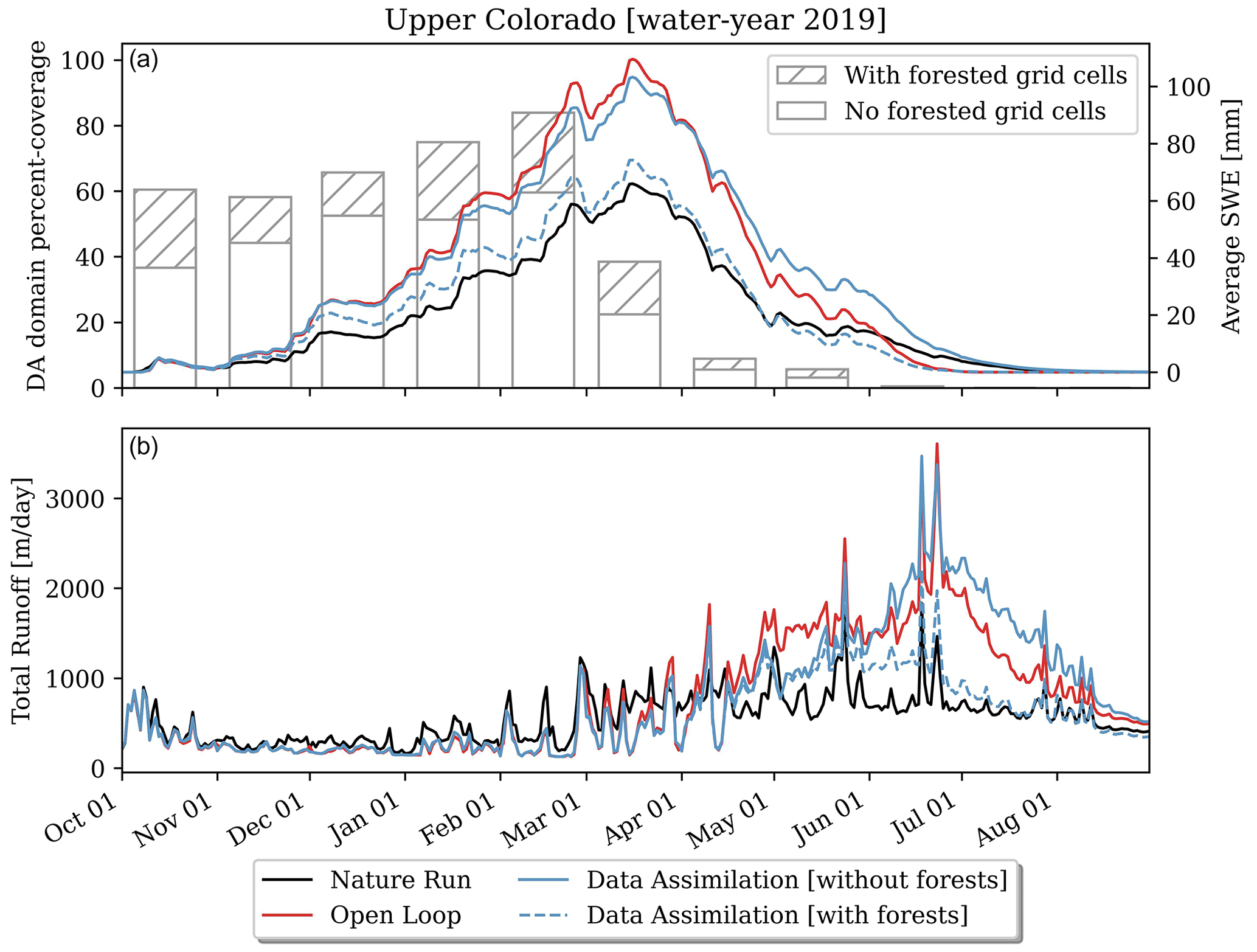
Figure 7Time series comparison of mean SWE (a) and total runoff (b) between the open loop, nature run, and simulations assimilating the synthetic observations, both with and without the forest strategy in the Upper Colorado. Hatched bars in (a) represent the monthly percentage of the Upper Colorado grid cells with no snowmelt. Solid bars also exclude grid cells with forest coverage.
Much like the Upper Colorado, SWE simulated by the open loop simulation in the Pacific Northwest (Fig. S7) was biased high for the entirety of the snow season. Both domains also had greater than 80 % synthetic snow observation coverage in March (including grid cells that filled snow estimates using the forest strategy), and as a result, the simulation with data assimilation using the forest strategy closely matched SWE from the nature run. However, both of these domains had a significant portion of the seasonal snowpack in forested land cover (the difference between the hatched and solid bars in Figs. 7 and S7). These grid cells had winter SWE estimates from the open loop simulation that were predominately high-biased (Figs. 3 and 5). Therefore, although data assimilation improved winter SWE in non-forested land cover types (Fig. 6), the simulation without the forest strategy caused little to no improvement in the simulated domain mean maximum SWE (Table 2). This highlights the value of the forest strategy used here (Fig. 2), which drew information from synthetic observations in relatively few nearby pixels to infer the mean snow volume in forested grid cells. Given the four hydrologic regions investigated in this study, a far smaller volume of snow existed in forested land cover for the California (Fig. S8) and Great Basin regions (Fig. S6), resulting in a DJF domain-mean SWE evolution that was more similar between the simulations with and without the forest strategy. We expect results in these domains to be more indicative of the value of winter SAR observations in less-vegetated snowy landscapes such as Tundra and Prairie snow regimes (Sturm and Liston, 2021).
Finally, the improvements to the spatial and temporal estimates of SWE discussed above had trickle-down improvements on simulated runoff. For example, in the Upper Colorado (Fig. 7), total annual runoff from the open loop simulation was biased high by approximately 35 % relative to the nature run. This error was driven mostly by high-biased winter snow accumulation, which nearly doubled the melt season (March–July) runoff estimated by the nature run simulation. Here, by assimilating the synthetic SWE observations and estimating forest snowpack from the relationship between modeled and observed SWE from the nearest canopy-free pixels, total annual streamflow in this domain was improved to within 1 %. Not only was domain total runoff improved, but the seasonal evolution of high and low flows vital for water management and planning was also improved. This improved the Nash–Sutcliffe efficiency (NSE) from −2.59 to 0.22 between the open loop simulation and simulation with data assimilation employing the forest strategy (Table 2). These results were similar for the Pacific Northwest, which had an NSE that improved from −0.17 to 0.39. However, due to the smaller changes to SWE and more-rapid snowmelt simulated by Noah-MP, changes to runoff from data assimilation in California and the Great Basin were small (Table 2), with improvements that were largely outweighed by the difference in snowmelt timing and rates between Noah-MP and SnowModel.
The differences between the open loop simulation and nature run in this study were representative of snow modeling errors common for continental and global-scale models used for seasonal to long-term future snow predictions (e.g., Franz et al., 2010; Garousi-Nejad and Tarboton, 2022; Kim et al., 2021; Liu et al., 2022). The greatest source of these snow modeling errors is commonly errors in meteorological forcing data, and in particular, biases in precipitation (Garousi-Nejad and Tarboton, 2022; Henn et al., 2018; Pflug et al., 2021; Raleigh and Lundquist, 2012; Wayand et al., 2013). These biases are especially prevalent in the portions of the earth's surface with the greatest volumes of snow, such as the tundra and montane regions (Kim et al., 2021), where ground observations and observation station maintenance are hindered by harsh winter conditions and inaccessibility. This suggests that the greatest need for improving global estimates of snow is improved estimates of snow accumulation in remote, under sampled landscapes. Here we expect that the SAR observations evaluated in this study could address these needs, thus providing a path forward for pairing common snow models with observations as a basis for determining global snow mass. For example, assimilating SAR observations at 10–14 d intervals with the observational error characteristics reported in Sect. 2.2, improved midlatitude winter SWE volume by approximately 22 %, on average (Table 2). In unforested landscapes, which account for the majority of the earth's snow water storage (Kim et al., 2021), assimilation improved the mean SWE bias at maximum SWE timing to within 1 %, on average, and reduced the standard deviation of errors by approximately 45 mm (∼85 %) (Fig. 6).
Despite the benefits discussed above, SAR observations have known limitations in forested landscapes where the canopy overstory obstructs retrievals from the underlying snowpack (Huang et al., 2019; Ruiz et al., 2022; Tsang et al., 2022). Therefore, this study was designed to investigate a forest strategy that uses the relationship between modeled SWE estimates and synthetic SWE observations from neighboring grid cells as the basis for inferring snow distribution in regions with forested land cover (Fig. 2). To focus on the benefits of this approach, we chose a domain (Fig. 1) that included both significant forest spatial coverage (22 %) with disproportionate amounts of winter snow (34 %) within the forested pixels (Fig. 6). Relative to the open loop simulation, the simulation with data assimilation and the forest strategy dramatically improved the spatial distribution of SWE (e.g., Figs. 3 and 4) and the resulting SWE biases at domain maximum snowpack timing (Fig. 5). In fact, in forested grid cells, the SWE on 13 March was only biased by 14 mm (mean absolute error of 27 mm), on average, for the simulation with data assimilation and the forest strategy, relative to the nature run. This was opposed to the open loop simulation, which was biased by 87 mm (mean absolute error of 111 mm) over the same regions and date. Despite the fact that the two simulations with data assimilation agreed in all grid cells except forested grid cells, the simulation employing the forest strategy had a mean absolute error (17 mm) across the full modeling region that was approximately 51 % smaller than the simulation without the forest strategy. Here we recognize that this study used a single date (13 March) to represent snow water resources at maximum SWE timing. However, the date of maximum SWE volume from the nature run varied by less than a week across the four hydrologic regions (11–16 March; Figs. 7, S6–S8). Therefore, this was a relevant date for model comparisons, especially given that water resource and allocation decisions in the western USA are often based on the volume of snow at maximum snow timing.
This research shows how a modeling framework and relatively few observations can be used to gap-fill estimates of snow in regions where remote sensing observations from a future platform may be most challenged. Despite the fact that snowpack with properties able to be retrieved by SAR instrumentation (i.e., canopy-free land cover and no snowmelt) sometimes only accounted for only small portions of a modeling domain (e.g., Fig. 7), SWE from the model and SAR observations in nearby canopy-free grid cells were predictive of the snow in forested grid cells. We hypothesize that this could have partly been driven by the 250 m resolution of synthetic observations and simulations. At this length scale, snow distribution is typically driven by processes like mesoscale weather patterns and their interaction (orographic lapse rates, wind loading and/or sheltering, terrain-shading, etc.) with static topographical features like elevation, slope, and aspect (e.g., Clark et al., 2011; Lehning et al., 2011; McGrath et al., 2018; Minder et al., 2008; Trujillo et al., 2007). However, we acknowledge that snow in forested and open grid cells is subject to different snow processes. In fact, the nature run simulation used here attempts to simulate snow-canopy interactions, such as snow interception and solar shading from the canopy overstory (Liston and Elder, 2006). Here, since we focus predominantly on model improvements from data assimilation in the SWE accumulation season, we hypothesize that the primary difference between SWE accumulation in forested pixels and the nearest canopy-free grid cells could be driven by canopy interception, or the lack thereof. In other words, inferring forested snowpack using the nearest canopy-free grid cells could bias snow in forested regions where snow processes differ slightly. While the forest strategy improved SWE simulated in forested grid cells at the date of maximum SWE volume, SWE was still biased high relative to the nature run (Fig. 6). We hypothesize that a correction factor, based on variables like forest canopy type, vegetation density, wind speed, and temperature during snowfall, all of which influence snow interception (Lundquist et al., 2021), could be used to facilitate the difference in snow accumulation expected between a forest pixel and SWE observations from nearby canopy-free grid cells. This approach will be a topic of future research. However, since errors with precipitation are often the overwhelming source of model errors, we hypothesize that the forest strategy (Fig. 2), which corrected modeled SWE in forested areas using the ratio between modeled and observed SWE in nearby open areas, was well suited to correct precipitation biases.
The results presented here are subject to a number of assumptions. These assumptions were intended to apply regionally consistent and conservative rules about how (1) synthetic SAR observations were generated and (2) the grid cells and time periods in which SAR observations occurred. For example, we used a 20 % and zero-mean random distribution of errors to generate observations from the nature run. We expect the error from a future satellite mission to be less than 20 % over the majority of snow covered regions (Sect. 2.2). However, observational biases may be more common in certain locations and periods based on snow depth, particularly in very shallow or very deep snowpacks, terrain characteristics, and vegetation characteristics. Additionally, the land cover classification used in this study (Fig. 1) was based on the dominant land cover type within each model grid cell, as defined from the North American Land Change Monitoring System (Latifovic et al., 2017). For forested grid cells, this included needleleaf, broadleaf, and mixed forest types. To be conservative, this study completely masked synthetic observations in 250 m grid cells classified as forest, thereby assuming (1) no observation capabilities in predominantly forested areas and (2) full observation capabilities in grid cells where forests were not the dominant land cover type. In reality, SAR may be able to achieve accurate snow retrievals in some forested-dominated regions based on the forest type, forest distribution, and canopy density (Tsang et al., 2022). Conversely, some regions with sparser or no forest cover may still have observation limitations based on the domain and snow characteristics mentioned above. The large domain used in this study also made tests over multiple years computationally challenging. Here the intent of this study was to investigate a strategy for deriving SWE corrections in difficult-to-observe forest landscapes, and we hypothesize that precipitation biases and the resulting modeled SWE accumulation could be improved to a similar degree in years with both larger and smaller snow volumes. Finally, while strategies for identifying and correcting systematic SAR observation errors are a topic of continued research (e.g., Durand et al., 2024; Singh et al., 2023), OSSEs are an inherently flexible framework for evaluating sensor utility, so future research could use the simulations performed here to test a wider array of sensor configurations and non-normal retrieval errors. Future work could build upon these results to investigate multiple years, perhaps considering warmer and/or drier snow years, when the role of snowpack for water supply and midwinter snowmelt and rain-on-snow frequency may be more likely to increase snowpack liquid water content, or years with late-season spring snow accumulation. Future research should also investigate other gap-filling approaches, like methods to infer SWE in grid cells where snowmelt is occurring and liquid water may prevent SAR retrievals, and gap-filling approaches using different window sizes and/or searching windows that more heavily weight unforested grid cells with similar characteristics (elevation, aspect, etc.).
This study tested a simple model setup using a popular land surface model (Noah-MP) and Kalman-based data assimilation procedure. This data assimilation procedure updated modeled snow states, like snow depth and SWE, based only on synthetic SWE observations at 10–14 d temporal frequencies where/when snowmelt was not occurring. Despite the limitations and assumptions discussed above, we expect that the results presented here could represent the lower boundary of performance that could be achieved from a real-time modeling framework that could accompany a space-borne SAR remote sensing platform. For example, many studies have demonstrated repeatable patterns of snow accumulation in years with similar winter meteorological characteristics (e.g., Deems et al., 2008; Pflug et al., 2022; Schirmer et al., 2011; Sturm and Wagner, 2010; Woodruff and Qualls, 2019). This suggests that retrospective information about snow distribution patterns in previous years could be used as the basis for extrapolating and updating snow model states in grid cells not covered by SAR observations on a given date. From the modeling perspective, only five ensemble members were used in the ensemble Kalman data assimilation (Sect. 2.3), whereas a larger ensemble of simulations may have improved uncertainty characterization of simulated snow and hydrologic states even more. This study also assumed that synthetic SAR observations were unable to observe snow in all forested landscapes, when retrievals of snow in forested stands could be achievable for some forested regions with smaller tree cover fractions and biomass (Montomoli et al., 2015; Tsang et al., 2022). Finally, the SAR configuration tested here had 10–14 d repeat times, but future satellite configurations with more-frequent observational repeats are possible and have been recommended by the 2018 Decadal Survey (NASM, 2018). Despite all of these conservative assumptions, the difference between the open loop simulation (representative of current modeling accuracies) and the simulation with synthetic observation data assimilation using the forest strategy demonstrated large-magnitude and widespread improvements to real-time estimates of winter SWE and the associated improvement to spring SWE and runoff. Therefore, we expect the findings of this study, particularly the strategy to extend the observational utility to forested areas, to significantly aid in the full exploitation of the information from a future SAR-based snow satellite mission.
Global estimates of snow volume and distribution have uncertainties stemming from limited snow observations and biases in meteorological forcing data. These uncertainties stress the need for a global snow-focused satellite remote sensing platform. Here we investigate the degree to which synthetic observations of SWE representative of a synthetic aperture radar remote sensing platform could correct common snow modeling errors and provide spatiotemporally continuous SWE estimates. We investigate this using an observing system simulation experiment, specifically investigating how much snow simulated using a widely used land surface model and meteorological forcing dataset could be improved by assimilating synthetic SAR observations of SWE.
The difference between the open loop simulation and the nature run was representative of common modeling errors. Snow simulated by the open loop simulation had larger winter snow extents and total snow volume that was biased high by approximately 35 %. The open loop simulation also simulated snow that was more spatially homogeneous, underestimating the variability across variations in topography and underestimating lower-elevation snowmelt from the nature run. Assimilating the synthetic SWE observations improved SWE simulated in the shrub, grass, crop, bare-ground, and wetland land cover types. In fact, SWE biases on the date of domain maximum SWE volume (13 March 2019) in these land cover types improved from 14 % for the open loop simulation to within 1 % after data assimilation. However, despite only covering 22 % of the study area, forested grid cells contained just over 34 % of the domain SWE on 13 March. The open loop simulation and the simulation with data assimilation without the forest strategy had SWE that was high biased by 150 % (87 mm), on average, in these forested grid cells. The relationship between modeled SWE and synthetic SWE observations in forested grid cells exhibited similarities with the nearest canopy-free grid cells. Therefore, SWE in forested regions was able to be inferred using the simple modeling framework and synthetic SAR observations from nearby canopy-free grid cells. In fact, the simulation with data assimilation using this forest gap-filling strategy substantially improved SWE biases to 4 % (∼22 % improvement) at maximum SWE timing, with an SWE mean absolute error of 17 mm (24 mm improvement) and spatial correlation of 0.91 (0.17 improvement) across the western USA.
Improvements in winter SWE accumulation also improved estimates of melt-season SWE evolution and total runoff in four major western USA hydrologic regions, even in periods when winter snowmelt greatly reduced the number of grid cells that could be observed by the synthetic SWE observations. In fact, in the Upper Colorado, melt season SWE biases improved from 63 % to less than 1 % after assimilation, and the runoff Nash–Sutcliffe efficiency improved from −2.59 to 0.22. These results demonstrate the value of SAR observations and simple spatial-filling strategies in grid cells where SAR retrievals could be obstructed by the canopy. Here we expect our results to represent a lower-boundary of model performance which could be improved further by more robust assimilation approaches, more-frequent SAR observations, further developments to SAR retrieval algorithms in forested landscapes, and adaptations to the forest gap-filling strategy developed here. However, our results also show that widespread improvements to global SWE could be available in near real-time provided data assimilation approaches and an SAR remote sensing platform.
The Land Information System (LIS; https://lis.gsfc.nasa.gov/, NASA, 2024a) framework used to perform the nature run, open loop, and data assimilation simulations from this study can be accessed from a GitHub public repository (https://github.com/NASA-LIS/LISF, NASA-LIS, 2024). Model documentation and LIS tutorials can also be accessed from this repository. Users are encouraged to reference Kumar et al. (2006) for more information on LIS. The Trade-space Analysis Tool for designing Constellations (TAT-C) tool is currently available upon request for federal employees and contractors (https://software.nasa.gov/software/GSC-18399-1, NASA, 2024b).
The model outputs and data necessary to reproduce the figures and statistics reported in this study can be found at https://www.hydroshare.org/resource/e0ad80f818bf4062a335e9e0d7362834/ (Pflug, 2023). This repository includes domain static variables, such as land cover, elevation, and spatial coordinates, in addition to model outputs of winter-average SWE, SWE at the date of maximum SWE volume (13 March 2019), and SWE and runoff aggregated across each region. MERRA-2 forcing data can be accessed from the Goddard Earth Sciences Data and Information Services Center (GES DISC, https://disc.gsfc.nasa.gov/; GES DISC, 2024), and ERA5 data can be accessed from the European Centre for Medium-Range Weather Forecasts climate data store (https://www.ecmwf.int/en/forecasts/dataset/ecmwf-reanalysis-v5; Copernicus Climate Change Service, 2024).
The supplement related to this article is available online at: https://doi.org/10.5194/hess-28-631-2024-supplement.
CMV and SVK coordinated the manuscript question and research methodology. SVK adapted LIS model source code to implement the forest gap-filling strategy in Sect. 2.4. MLW set up the model domains and model configurations, and performed the open loop simulation. EC assisted with generating the synthetic SWE observations. With assistance from KRA, JMP performed code developments for the simulations using both the Noah-MP and coupled SnowModel models. KRA implemented the SnowModel code and parameters into LIS and LDT. JMP also performed the nature run and both data assimilation simulations. The manuscript was developed with text, figures, and feedback from all coauthors.
The contact author has declared that none of the authors has any competing interests.
Publisher’s note: Copernicus Publications remains neutral with regard to jurisdictional claims made in the text, published maps, institutional affiliations, or any other geographical representation in this paper. While Copernicus Publications makes every effort to include appropriate place names, the final responsibility lies with the authors.
We acknowledge Ethan Gutmann, Ross Mower, and Glen Liston for supporting the integration of the SnowModel distributed model into LIS.
This work was supported by funding from the NASA Terrestrial Hydrology program, and the NASA Advanced Information Systems Technology Program (grant nos. AIST-18-0045 and 21-AIST21_2-0055). Computing was supported by the NASA Center for Climate Simulation (NCCS).
This paper was edited by Shraddhanand Shukla and reviewed by three anonymous referees.
Arsenault, K. R., Wrzesien, M., Gutmann, E. D., Vuyovich, C., Liston, G. E., Mower, R., Reinking, A., Newman, A. J., Kumar, S. V., Wang, S., Navari, M., Forman, B. A., and Jessica, L.: Implementing SnowModel into the Land Information System Framework to Support High Resolution Modeling of Snow Heterogeneity, Presented at the AGU Fall Meeting 2021, AGU, 13–17 December 2021, New Orleans, LA, https://ui.adsabs.harvard.edu/abs/2021AGUFM.C35G0945A/abstract (last access: 9 February 2024), 2021.
Barnett, T. P., Adam, J. C., and Lettenmaier, D. P.: Potential impacts of a warming climate on water availability in snow-dominated regions, Nature, 438, 303, https://doi.org/10.1038/nature04141, 2005.
Barry, R. G.: The Role of Snow and Ice in the Global Climate System: A Review, Polar Geography, 26, 235–246, https://doi.org/10.1080/789610195, 2002.
Best, M. J., Pryor, M., Clark, D. B., Rooney, G. G., Essery, R. L. H., Ménard, C. B., Edwards, J. M., Hendry, M. A., Porson, A., Gedney, N., Mercado, L. M., Sitch, S., Blyth, E., Boucher, O., Cox, P. M., Grimmond, C. S. B., and Harding, R. J.: The Joint UK Land Environment Simulator (JULES), model description – Part 1: Energy and water fluxes, Geosci. Model Dev., 4, 677–699, https://doi.org/10.5194/gmd-4-677-2011, 2011.
Beven, K. J., Kirkby, M. J., Freer, J. E., and Lamb, R.: A history of TOPMODEL, Hydrol. Earth Syst. Sci., 25, 527–549, https://doi.org/10.5194/hess-25-527-2021, 2021.
Cho, E., Vuyovich, C. M., Kumar, S. V., Wrzesien, M. L., and Kim, R. S.: Evaluating the utility of active microwave observations as a snow mission concept using observing system simulation experiments, The Cryosphere, 17, 3915–3931, https://doi.org/10.5194/tc-17-3915-2023, 2023.
Clark, M. P., Hendrikx, J., Slater, A. G., Kavetski, D., Anderson, B., Cullen, N. J., Kerr, T., Hreinsson, E. Ö., and Woods, R. A.: Representing spatial variability of snow water equivalent in hydrologic and land-surface models: A review, Water Resour. Res., 47, W07539, https://doi.org/10.1029/2011WR010745, 2011.
Cosgrove, B. A., Lohmann, D., Mitchell, K. E., Houser, P. R., Wood, E. F., Schaake, J. C., Robock, A., Marshall, C., Sheffield, J., Duan, Q., and Luo, L.: Real-time and retrospective forcing in the North American Land Data Assimilation System (NLDAS) project, J. Geophys. Res.-Atmos., 108, 8842, https://doi.org/10.1029/2002JD003118, 2003.
De Lannoy, G. J. M., Reichle, R. H., Arsenault, K. R., Houser, P. R., Kumar, S., Verhoest, N. E. C., and Pauwels, V. R. N.: Multiscale assimilation of Advanced Microwave Scanning Radiometer–EOS snow water equivalent and Moderate Resolution Imaging Spectroradiometer snow cover fraction observations in northern Colorado, Water Resour. Res., 48, W01522, https://doi.org/10.1029/2011WR010588, 2012.
Deems, J. S., Fassnacht, S. R., and Elder, K. J.: Interannual Consistency in Fractal Snow Depth Patterns at Two Colorado Mountain Sites, J. Hydrometeor., 9, 977–988, https://doi.org/10.1175/2008JHM901.1, 2008.
Derksen, C., Lemmetyinen, J., Toose, P., Silis, A., Pulliainen, J., and Sturm, M.: Physical properties of arctic versus subarctic snow: Implications for high latitude passive microwave snow water equivalent retrievals, J. Geophys. Res.-Atmos., 119, 7254–7270, https://doi.org/10.1002/2013JD021264, 2014.
Durand, M., Johnson, J. T., Dechow, J., Tsang, L., Borah, F., and Kim, E. J.: Retrieval of snow water equivalent from dual-frequency radar measurements: using time series to overcome the need for accurate a priori information, The Cryosphere, 18, 139–152, https://doi.org/10.5194/tc-18-139-2024, 2024.
Copernicus Climate Change Service: ERA5 data, European Centre for Medium-Range Weather Forecasts climate data store [data set], https://www.ecmwf.int/en/forecasts/dataset/ecmwf-reanalysis-v5 (last access: 9 February 2024), 2024.
Ek, M. B., Mitchell, K. E., Lin, Y., Rogers, E., Grunmann, P., Koren, V., Gayno, G., and Tarpley, J. D.: Implementation of Noah land surface model advances in the National Centers for Environmental Prediction operational mesoscale Eta model, J. Geophys. Res.-Atmos., 108, 8851, https://doi.org/10.1029/2002JD003296, 2003.
Errico, R. M., Yang, R., Masutani, M., and Woollen, J. S.: The estimation of analysis error characteristics using an observation systems simulation experiment, Meteorol. Z., 16, 695–708, 2007.
Fang, Y., Liu, Y., and Margulis, S. A.: A western United States snow reanalysis dataset over the Landsat era from water eyars 1985 to 2021, Sci. Data, 9, 677, https://doi.org/10.1038/s41597-022-01768-7, 2022.
Foster, J. L., Sun, C., Walker, J. P., Kelly, R., Chang, A., Dong, J., and Powell, H.: Quantifying the uncertainty in passive microwave snow water equivalent observations, Remote Sens. Environ., 94, 187–203, https://doi.org/10.1016/j.rse.2004.09.012, 2005.
Franz, K. J., Butcher, P., and Ajami, N. K.: Addressing snow model uncertainty for hydrologic prediction, Adv. Water Resour., 33, 820–832, https://doi.org/10.1016/j.advwatres.2010.05.004, 2010.
Garnaud, C., Bélair, S., Carrera, M. L., Derksen, C., Bilodeau, B., Abrahamowicz, M., Gauthier, N., and Vionnet, V.: Quantifying Snow Mass Mission Concept Trade-Offs Using an Observing System Simulation Experiment, J. Hydrometeorol., 20, 155–173, https://doi.org/10.1175/JHM-D-17-0241.1, 2019.
Garousi-Nejad, I. and Tarboton, D. G.: A comparison of National Water Model retrospective analysis snow outputs at snow telemetry sites across the Western United States, Hydrol. Process., 36, e14469, https://doi.org/10.1002/hyp.14469, 2022.
Gelaro, R., McCarty, W., Suárez, M.J., Todling, R., Molod, A., Takacs, L., Randles, C. A., Darmenov, A., Bosilovich, M. G., Reichle, R., Wargan, K., Coy, L., Cullather, R., Draper, C., Akella, S., Buchard, V., Conaty, A., Silva, A. M. da, Gu, W., Kim, G.-K., Koster, R., Lucchesi, R., Merkova, D., Nielsen, J. E., Partyka, G., Pawson, S., Putman, W., Rienecker, M., Schubert, S. D., Sienkiewicz, M., and Zhao, B.: The Modern-Era Retrospective Analysis for Research and Applications, Version 2 (MERRA-2), J. Climate, 30, 5419–5454, https://doi.org/10.1175/JCLI-D-16-0758.1, 2017.
GES DISC: MERRA-2 forcing data, Goddard Earth Sciences Data and Information Services Center [data set], https://disc.gsfc.nasa.gov/ (last access: 9 February 2024), 2024.
Henn, B., Newman, A. J., Livneh, B., Daly, C., and Lundquist, J. D.: An assessment of differences in gridded precipitation datasets in complex terrain, J. Hydrol., 556, 1205–1219, https://doi.org/10.1016/j.jhydrol.2017.03.008, 2018.
Hersbach, H., Bell, B., Berrisford, P., Hirahara, S., Horányi, A., Muñoz-Sabater, J., Nicolas, J., Peubey, C., Radu, R., Schepers, D., Simmons, A., Soci, C., Abdalla, S., Abellan, X., Balsamo, G., Bechtold, P., Biavati, G., Bidlot, J., Bonavita, M., De Chiara, G., Dahlgren, P., Dee, D., Diamantakis, M., Dragani, R., Flemming, J., Forbes, R., Fuentes, M., Geer, A., Haimberger, L., Healy, S., Hogan, R. J., Hólm, E., Janisková, M., Keeley, S., Laloyaux, P., Lopez, P., Lupu, C., Radnoti, G., de Rosnay, P., Rozum, I., Vamborg, F., Villaume, S., and Thépaut, J.-N.: The ERA5 global reanalysis, Q. J. Roy. Meteor. Soc., 146, 1999–2049, https://doi.org/10.1002/qj.3803, 2020.
Hiemstra, C. A., Liston, G. E., and Reiners, W. A.: Snow Redistribution by Wind and Interactions with Vegetation at Upper Treeline in the Medicine Bow Mountains, Wyoming, U.S.A., Arct. Antarct. Alp. Res., 34, 262–273, https://doi.org/10.1080/15230430.2002.12003493, 2002.
Huang, H., Tsang, L., Colliander, A., and Yueh, S. H.: Propagation of Waves in Randomly Distributed Cylinders Using Three-Dimensional Vector Cylindrical Wave Expansions in Foldy–Lax Equations, IEEE Journal on Multiscale and Multiphysics Computational Techniques 4, 214–226, https://doi.org/10.1109/JMMCT.2019.2948022, 2019.
Kim, R. S., Kumar, S., Vuyovich, C., Houser, P., Lundquist, J., Mudryk, L., Durand, M., Barros, A., Kim, E. J., Forman, B. A., Gutmann, E. D., Wrzesien, M. L., Garnaud, C., Sandells, M., Marshall, H.-P., Cristea, N., Pflug, J. M., Johnston, J., Cao, Y., Mocko, D., and Wang, S.: Snow Ensemble Uncertainty Project (SEUP): quantification of snow water equivalent uncertainty across North America via ensemble land surface modeling, The Cryosphere, 15, 771–791, https://doi.org/10.5194/tc-15-771-2021, 2021.
Koster, R. D., Suarez, M. J., Ducharne, A., Stieglitz, M., and Kumar, P.: A catchment-based approach to modeling land surface processes in a general circulation model: 1. Model structure. J. Geophys. Res.-Atmos., 105, 24809–24822, https://doi.org/10.1029/2000JD900327, 2000.
Koster, R. D., Mahanama, S. P. P., Livneh, B., Lettenmaier, D. P., and Reichle, R. H.: Skill in streamflow forecasts derived from large-scale estimates of soil moisture and snow, Nat. Geosci., 3, 613–616, https://doi.org/10.1038/ngeo944, 2010.
Kumar, S. V., Peters-Lidard, C. D., Tian, Y., Houser, P. R., Geiger, J., Olden, S., Lighty, L., Eastman, J. L., Doty, B., Dirmeyer, P., Adams, J., Mitchell, K., Wood, E. F., and Sheffield, J.: Land information system: An interoperable framework for high resolution land surface modeling, Environ. Model. Softw., 21, 1402–1415, https://doi.org/10.1016/j.envsoft.2005.07.004, 2006.
Kumar, S. V., Peters-Lidard, C. D., Mocko, D., and Tian, Y.: Multiscale Evaluation of the Improvements in Surface Snow Simulation through Terrain Adjustments to Radiation, J. Hydrometeorol., 14, 220–232, https://doi.org/10.1175/JHM-D-12-046.1, 2013.
Kumar, S. V., Kolassa, J., Reichle, R., Crow, W., de Lannoy, G., de Rosnay, P., MacBean, N., Girotto, M., Fox, A., Quaife, T., Draper, C., Forman, B., Balsamo, G., Steele-Dunne, S., Albergel, C., Bonan, B., Calvet, J.-C., Dong, J., Liddy, H., and Ruston, B.: An Agenda for Land Data Assimilation Priorities: Realizing the Promise of Terrestrial Water, Energy, and Vegetation Observations From Space, J. Adv. Model. Earth Sy., 14, e2022MS003259, https://doi.org/10.1029/2022MS003259, 2022.
Kwon, Y., Yoon, Y., Forman, B. A., Kumar, S. V., and Wang, L.: Quantifying the observational requirements of a space-borne LiDAR snow mission, J. Hydrol., 601, 126709, https://doi.org/10.1016/j.jhydrol.2021.126709, 2021.
Lahmers, T. M., Kumar, S. V., Rosen, D., Dugger, A., Gochis, D. J., Santanello, J. A., Gangodagamage, C., and Dunlap, R.: Assimilation of NASA's Airborne Snow Observatory Snow Measurements for Improved Hydrological Modeling: A Case Study Enabled by the Coupled LIS/WRF-Hydro System, Water Resour. Res., 58, e2021WR029867, https://doi.org/10.1029/2021WR029867, 2022.
Latifovic, R., Pouliot, D., and Olthof, I.: Circa 2010 Land Cover of Canada: Local optimization methodology and product development, Remote Sens., 9, 11, https://doi.org/10.3390/rs9111098, 2017.
Le Moigne, J., Dabney, P., de Weck, O., Foreman, V., Grogan, P., Holland, M., Hughes, S., and Nag, S.: Tradespace analysis tool for designing constellations (TAT-C), in: 2017 IEEE International Geoscience and Remote Sensing Symposium (IGARSS), IEEE, 1181–1184, https://doi.org/10.1109/IGARSS.2017.8127168, 2017.
Lehning, M., Grünewald, T., and Schirmer, M.: Mountain snow distribution governed by an altitudinal gradient and terrain roughness, Geophys. Res. Lett., 38, L19504, https://doi.org/10.1029/2011GL048927, 2011.
Li, D., Wrzesien, M. L., Durand, M., Adam, J., and Lettenmaier, D. P.: How much runoff originates as snow in the western United States, and how will that change in the future?, Geophys. Res. Lett., 44, 6163–6172, https://doi.org/10.1002/2017GL073551, 2017.
Liang, X., Lettenmaier, D. P., Wood, E. F., and Burges, S. J.: A simple hydrologically based model of land surface water and energy fluxes for general circulation models, J. Geophys. Res.-Atmos., 99, 14415–14428, https://doi.org/10.1029/94JD00483, 1994.
Lievens, H., Demuzere, M., Marshall, H. P., Reichle, R. H., Brucker, L., de Rosnay, P., Dumont, M., Girotto, M., Immerzeel, W. W., Jonas, T., Kim, E. J., Koch, I., Marty, C., Saloranta, T., Schober, J., and De Lannoy, G. J. M.: Snow depth variability in the Northern Hemisphere mountains observed from space, Nat. Commun., 10, 4629, https://doi.org/10.1038/s41467-019-12566-y, 2019.
Liston, G. E. and Elder, K.: A Distributed Snow-Evolution Modeling System (SnowModel), J. Hydrometeorol., 7, 1259–1276, https://doi.org/10.1175/JHM548.1, 2006.
Liston, G. E., Perham, C. J., Shideler, R. T., and Cheuvront, A. N.: Modeling snowdrift habitat for polar bear dens, Ecol. Model., 320, 114–134, https://doi.org/10.1016/j.ecolmodel.2015.09.010, 2016.
Liu, Y., Fang, Y., Li, D., and Margulis, S. A.: How well do global snow products characterize snow storage in high mountain Asia?, Geophys. Res. Lett., 49, e2022GL100082, https://doi.org/10.1029/2022GL100082, 2022.
Livneh, B. and Badger, A. M.: Drought less predictable under declining future snowpack, Nat. Clim. Chang., 10, 452–458, https://doi.org/10.1038/s41558-020-0754-8, 2020.
Lundquist, J. D., Dickerson-Lange, S., Gutmann, E., Jonas, T., Lumbrazo, C., and Reynolds, D.: Snow interceptions modelling: Isolated observations have led to many land surface models lacking appropriate temperature sensitivities, Hydrol. Process., 35, 7, https://doi.org/10.1002/hyp.14274, 2021.
Mahoney, P. J., Liston, G. E., LaPoint, S., Gurarie, E., Mangipane, B., Wells, A. G., Brinkman, T. J., Eitel, J. U. H., Hebblewhite, M., Nolin, A. W., Boelman, N., and Prugh, L. R.: Navigating snowscapes: scale-dependent responses of mountain sheep to snowpack properties, Ecol. Appl., 28, 1715–1729, https://doi.org/10.1002/eap.1773, 2018.
McGrath, D., Sass, L., O'Neel, S., McNeil, C., Candela, S. G., Baker, E. H., and Marshall, H.-P.: Interannual snow accumulation variability on glaciers derived from repeat, spatially extensive ground-penetrating radar surveys, The Cryosphere, 12, 3617–3633, https://doi.org/10.5194/tc-12-3617-2018, 2018.
Mernild, S. H., Liston, G. E., Hiemstra, C., and Wilson, R.: The Andes Cordillera. Part III: glacier surface mass balance and contribution to sea level rise (1979–2014), Int. J. Climatol., 37, 3154–3174, https://doi.org/10.1002/joc.4907, 2017.
Minder, J. R., Durran, D. R., Roe, G. H., and Anders, A. M.: The climatology of small-scale orographic precipitation over the Olympic Mountains: Patterns and processes, Q. J. Roy. Meteor. Soc., 134, 817–839, https://doi.org/10.1002/qj.258, 2008.
Montomoli, F., Macelloni, G., Brogioni, M., Lemmetyinen, J., Cohen, J., and Rott, H.: Observations and simulation of multifrequency SAR data over a snow-covered boreal forest, IEEE J. Sel. Top. Appl., 9, 1216–1228, 2015.
NASA: LIS Framework, https://lis.gsfc.nasa.gov/ (last access: 9 February 2024), 2024.
NASA: Vehicle management space air ground Trade-space Analysis Tool for designing Constellations (TAT-C) – Version 2.0 (GSC-18399-1) https://software.nasa.gov/software/GSC-18399-1 last access: 9 February 2024), 2024.
NASA-LIS: LISF, GitHub [code], https://github.com/NASA-LIS/LISF (last access: 9 February 2024), 2024.
NASM: National Academies of Sciences, Engineering, and Medicine: Thriving on our changing planet: A decadal strategy for Earth observation from space, Washington, DC, The National Academies Press, https://doi.org/10.17226/24938, 2018.
Niu, G., Yang, Z., Mitchell, K. E., Chen, F., Ek, M. B., Barlage, M., Kumar, A., Manning, K., Niyogi, D., Rosero, E., Tewari, M., and Xia, Y.: The community Noah land surface model with multiparameterization options (Noah-MP): 1. Model description and evaluation with local-scale measurements, J. Geophys. Res.-Atmos., 116, D12109, https://doi.org/10.1029/2010JD015139, 2011.
Niu, G.-Y. and Yang, Z.-L.: Effects of vegetation canopy processes on snow surface energy and mass balances, J. Geophys. Res.-Atmos., 109, D23111, https://doi.org/10.1029/2004JD004884, 2004.
Painter, T. H., Berisford, D. F., Boardman, J. W., Bormann, K. J., Deems, J. S., Gehrke, F., Hedrick, A., Joyce, M., Laidlaw, R., Marks, D., Mattmann, C., McGurk, B., Ramirez, P., Richardson, M., Skiles, S. M., Seidel, F. C., and Winstral, A.: The Airborne Snow Observatory: Fusion of scanning lidar, imaging spectrometer, and physically-based modeling for mapping snow water equivalent and snow albedo, Remote Sens. Environ., 184, 139–152, https://doi.org/10.1016/j.rse.2016.06.018, 2016.
Pflug, J. M.: Pflug et al. (2023) – Model configuration and outputs, HydroShare [data set], http://www.hydroshare.org/resource/e0ad80f818bf4062a335e9e0d7362834 (last access: 9 February 2024), 2023.
Pflug, J. M., Hughes, M., and Lundquist, J. D.: Downscaling snow deposition using historic snow depth patterns: Diagnosing limitations from snowfall biases, winter snow losses, and interannual snow pattern repeatability, Water Resour. Res., e2021WR029999, https://doi.org/10.1029/2021WR029999, 2021.
Pflug, J. M., Margulis, S. A., and Lundquist, J. D.: Inferring watershed-scale mean snowfall magnitude and distribution using multidecadal snow reanalysis patterns and snow pillow observations, Hydrol. Process., 36, e14581, 2022.
Raleigh, M. S. and Lundquist, J. D.: Comparing and combining SWE estimates from the SNOW-17 model using PRISM and SWE reconstruction, Water Resour. Res., 48, W01506, https://doi.org/10.1029/2011WR010542, 2012.
Reichle, R. H., McLaughlin, D. B., and Entekhabi, D.: Hydrologic Data Assimilation with the Ensemble Kalman Filter, Mon. Weather Rev., 130, 103–114, https://doi.org/10.1175/1520-0493(2002)130<0103:HDAWTE>2.0.CO;2, 2002.
Rott, H., Yueh, S. H., Cline, D. W., Duguay, C., Essery, R., Haas, C., Hélière, F., Kern, M., Macelloni, G., Malnes, E., and Thompson, A.: Cold regions hydrology high-resolution observatory for snow and cold land processes, P. IEEE, 98, 752–765, 2010.
Rott, H., Duguay, C., Etchevers, P., Essery, R., Hajnsek, I., Macelloni, G., Malnes, E., and Pulliainen, J.: CoReH2O Report for mission selection: An Earth Explorer to observe snow and ice, Tech. rep., European Space Agency, https://earth.esa.int/eogateway/documents/20142/37627/CoReH 2O-Report-for-Mission-Selection-An-Earth-Explorer-to-observe-snow-and-ice.pdf (last access: 9 Feburary 2024), 2012.
Ruiz, J. J., Lemmetyinen, J., Kontu, A., Tarvainen, R., Vehmas, R., Pulliainen, J., and Praks, J.: Investigation of Environmental Effects on Coherence Loss in SAR Interferometry for Snow Water Equivalent Retrieval, IEEE T. Geosci. Remote, 60, 1–15, https://doi.org/10.1109/TGRS.2022.3223760, 2022.
Schirmer, M., Wirz, V., Clifton, A., and Lehning, M.: Persistence in intra-annual snow depth distribution: 1. Measurements and topographic control: Persistent Snow Depth Development, 1., Water Resour. Res., 47, W09516, https://doi.org/10.1029/2010WR009426, 2011.
Singh, S., Durand, M., Kim, E., and Barros, A. P.: Bayesian physical–statistical retrieval of snow water equivalent and snow depth from X- and Ku-band synthetic-aperture-radar demonstration using airborne SnowSAR in SnowEx17, EGUsphere [preprint], https://doi.org/10.5194/egusphere-2023-1987, 2023.
Sturm, M. and Liston, G. E.: Revisiting the Global Seasonal Snow Classification: An Updated Dataset for Earth System Applications, J. Hydrometeorol., 22, 2917–2938, https://doi.org/10.1175/JHM-D-21-0070.1, 2021.
Sturm, M. and Wagner, A. M.: Using repeated patterns in snow distribution modeling: An Arctic example, Water Resour. Res., 46, W12559, https://doi.org/10.1029/2010WR009434, 2010.
Terzago, S., Bongiovanni, G., and von Hardenberg, J.: Seasonal forecasting of snow resources at Alpine sites, Hydrol. Earth Syst. Sci., 27, 519–542, https://doi.org/10.5194/hess-27-519-2023, 2023.
Trujillo, E., Ramírez, J. A., and Elder, K. J.: Topographic, meteorologic, and canopy controls on the scaling characteristics of the spatial distribution of snow depth fields, Water Resour. Res., 43, W07409, https://doi.org/10.1029/2006WR005317, 2007.
Tsang, L., Durand, M., Derksen, C., Barros, A. P., Kang, D.-H., Lievens, H., Marshall, H.-P., Zhu, J., Johnson, J., King, J., Lemmetyinen, J., Sandells, M., Rutter, N., Siqueira, P., Nolin, A., Osmanoglu, B., Vuyovich, C., Kim, E., Taylor, D., Merkouriadi, I., Brucker, L., Navari, M., Dumont, M., Kelly, R., Kim, R. S., Liao, T.-H., Borah, F., and Xu, X.: Review article: Global monitoring of snow water equivalent using high-frequency radar remote sensing, The Cryosphere, 16, 3531–3573, https://doi.org/10.5194/tc-16-3531-2022, 2022.
Wayand, N. E., Hamlet, A. F., Hughes, M., Feld, S. I., and Lundquist, J. D.: Intercomparison of Meteorological Forcing Data from Empirical and Mesoscale Model Sources in the North Fork American River Basin in Northern Sierra Nevada, California, J. Hydrometeorol., 14, 677–699, https://doi.org/10.1175/JHM-D-12-0102.1, 2013.
Woodruff, C. D. and Qualls, R. J.: Recurrent Snowmelt Pattern Synthesis using Principal Component Analysis of Multi-Year Remotely Sensed Snow Cover, Water Resour. Res., 55, 6869–6885, https://doi.org/10.1029/2018WR024546, 2019.
Wrzesien, M., Kumar, S. V., Vuyovich, C., Kim, R. S., Cho, E., Pflug, J. M., Konapala, G., and Arsenault, K. R.: Merging remote sensing and models to improve performance and accessibility of snow information, AGU Fall Meeting, Conference on Hydrology, 12–16 December 2022, Chicago, IL, 2022.
Wrzesien, M. L., Kumar, S., Vuyovich, C., Gutmann, E. D., Kim, R. S., Forman, B. A., Durand, M., Raleigh, M. S., Webb, R., and Houser, P.: Development of a “Nature Run” for Observing System Simulation Experiments (OSSEs) for Snow Mission Development, J. Hydrometeorol., 23, 351–375, https://doi.org/10.1175/JHM-D-21-0071.1, 2022.
Ying, Y.: Assimilating Observations with Spatially Correlated Errors Using a Serial Ensemble Filter with a Multiscale Approach, Mon. Weather Rev., 148, 3397–3412, https://doi.org/10.1175/MWR-D-19-0387.1, 2020.
Yu, L., Fennel, K., Wang, B., Laurent, A., Thompson, K. R., and Shay, L. K.: Evaluation of nonidentical versus identical twin approaches for observation impact assessments: an ensemble-Kalman-filter-based ocean assimilation application for the Gulf of Mexico, Ocean Sci., 15, 1801–1814, https://doi.org/10.5194/os-15-1801-2019, 2019.
Yueh, S. H., Dinardo, S. J., Akgiray, A., West, R., Cline, D. W., and Elder, K.: Airborne Ku-band polarimetric radar remote sensing of terrestrial snow cover, IEEE T. Geosci. Remote, 47, 3347–3364, 2009.
Zhu, J., Tan, S., King, J., Derksen, C., Lemmetyinen, J., and Tsang, L.: Forward and inverse radar modeling of terrestrial snow using SnowSAR Data, IEEE T. Geosci. Remote, 56, 7122–7132, https://doi.org/10.1109/TGRS.2018.2848642, 2018.
Zhu, J., Tan, S., Tsang, L., Kang, D. K., and Kim, E.: Snow water equivalent retrieval using active and passive microwave observations, Water Resour. Res., 57, e2020WR027563, https://doi.org/10.1029/2020WR027563, 2021.