the Creative Commons Attribution 4.0 License.
the Creative Commons Attribution 4.0 License.
 | 08 Feb 2024
Technical Note: Resolution enhancement of flood inundation grids
Guy Schumann
Heiko Apel
Heidi Kreibich
Bruno Merz
High-resolution flood maps are needed for more effective flood risk assessment and management. Producing these directly with hydrodynamic models is slow and computationally prohibitive at large scales. Here we demonstrate a new algorithm for post-processing low-resolution inundation layers by using high-resolution terrain models to disaggregate or downscale. The new algorithm is roughly 8 times faster than state-of-the-art algorithms and shows a slight improvement in accuracy when evaluated against observations of a recent flood using standard performance metrics. Qualitatively, the algorithm generates more physically coherent flood maps in some hydraulically challenging regions compared to the state of the art. The algorithm developed here is open source and can be applied in conjunction with a low-resolution hydrodynamic model and a high-resolution DEM to rapidly produce high-resolution inundation maps. For example, in our case study with a river reach of 20 km, the proposed algorithm generated a 4 m resolution inundation map from 32 m hydrodynamic model outputs in 33 s compared to a 4 m hydrodynamic model runtime of 34 min. This 60-fold improvement in runtime is associated with a 25 % increase in RMSE when compared against the 4 m hydrodynamic model results and observations of a recent flood. Substituting downscaling into flood risk model chains for high-resolution modelling has the potential to drastically improve the efficiency of inundation map production and increase the lead time of impact-based forecasts, helping more at-risk communities prepare for and mitigate flood damages.
- Article
(7013 KB) - Full-text XML
-
Supplement
(2176 KB) - BibTeX
- EndNote


Over the past decade, there has been significant progress in the development and implementation of flood models for large continental river basins and at the global scale. This is due to several factors including the rise in flood-related disaster damages, advancements in computing, and the availability and quality of global datasets (Ward et al., 2020; Nones and Caviedes‐Voullième, 2020). As these models underpin risk management activities, like early warning, land use planning, and disaster response, their accuracy and efficiency are important considerations for improving disaster resilience (De Moel et al., 2009).
Because of the computational demands of hydrodynamic models, resolution has been extensively studied and found to be one of the parameters of most importance for accuracy (Horritt and Bates, 2001; Fewtrell et al., 2008; Savage et al., 2016; Papaioannou et al., 2016; Alipour et al., 2022), with most finding inundation area and flood depth overestimated at coarser resolutions (Saksena and Merwade, 2015; Mohanty et al., 2020; Ghimire and Sharma, 2021; Muthusamy et al., 2021; Banks et al., 2015). In a study comparing fine and coarse models with resolution ranging from 1 m to 50 m and identical roughness, Muthusamy et al. (2021) used separate resolutions for the channel and floodplain. They found an overestimate in water depths and attributed it to the poorly defined coarse river channel (e.g., thalweg depth underestimated or steep bank misrepresentation) and a subsequent reduction in conveyance (Muthusamy et al., 2021).
There are three primary hazard grids included in most flood risk models: water depth or water surface height (WSH), water surface elevation (WSE), and the ground elevations (DEM) which can be related by . Often, WSE or WSH grids are produced from a hydraulic analysis or some model structured on the DEM, leading to a natural pairing of resolution, datum, and domain (i.e., the real-world region associated with the model). For large-scale studies, the resolution (s) of the DEM is relatively coarse (30–100 m), resulting from the process and data used to construct the terrain model or from some post-process upscaling introduced to obtain the resolution desired by the hydraulic analysis (i.e., coarsening model resolution to reduce complexity and runtime). For this latter case or any case where supplementary fine-resolution (s1) DEM grids are available, applications like flood damage modelling or impact-based forecasting may benefit from enhancing WSE grids through downscaling or disaggregation to obtain a finer resolution without the need for expensive or unstable hydrodynamic modelling. Unlike super-resolution techniques, which seek a high-resolution image from a single low-resolution image (Dong et al., 2015), flood hazard grid downscaling is a well-posed problem that uses the high-resolution DEMs1 and simple hydraulic assumptions to seek the WSEs1 grid that would be generated by an otherwise equivalent high-resolution hydrodynamic model.
While many flood risk model studies maintain a single resolution throughout the analysis (Hall et al., 2005; Sairam et al., 2021), examples of both upscaling and downscaling hazard grids are common. Upscaling, where hazard model output grids are post-processed to coarsen resolution, is generally undertaken to facilitate intersection with some exposure data, which is generally the most coarse data grid in flood risk model chains. This upscaling is achieved either through simple averaging (Seifert et al., 2010; Sieg and Thieken, 2022) or some unspecified method (Thieken et al., 2016; Jongman et al., 2012). Examples of downscaling in the literature may employ it to reverse some earlier coarsening which was applied to improve hydrodynamic model stability or efficiency (Schumann et al., 2014; Sampson et al., 2015) or enhance some remote-sensing-derived inundation product (Fluet-Chouinard et al., 2015; Aires et al., 2017).
In the first and only study (we are aware of) to investigate downscaling 2D calibrated hydrodynamic models, Schumann et al. (2014) developed a method using a nearest-neighbour search with N4(P) adjacency (querying values from only the N, S, E, and W adjacent or neighbouring cells rather than N8(P) which queries all eight neighbouring cells) and a search radius of half the coarse resolution. The researchers tested their algorithm using two models: a fine model with a 30 m resolution and a coarse model with a 600 m resolution, each calibrated separately. When comparing the downscaled grid to the results of the fine hydrodynamic model, they discovered an overestimate in water levels and negligible differences in volume. This method substantially improved computation times (compared to hydrodynamic modelling) and provided the basis for some large-scale flood models (Sampson et al., 2015; Bates et al., 2021). The CaMa-Flood project (Yamazaki et al., 2011) has developed a FORTRAN script with a similar algorithm to downscale results of their global river model; however, this script has not been described in any publication we are aware of. With the objective of operationalizing a 2D hydrodynamic model, Fraehr et al. (2023) developed a modelling framework that integrates a “Gaussian process” learning model with a low-fidelity hydrodynamic model to yield high-resolution depth and inundation estimates.
As part of their work to enhance the VIIRS (Visible Infrared Imaging Radiometer Suite) 375 m resolution near real-time global flood inundation product, Li et al. (2022) developed a seven-stage downscaling and correction pipeline. Leveraging global datasets for tree cover, land cover, permanent water bodies, and river networks, VIIRS water fractions were first converted to water levels and then corrected using simple hydraulic assumptions. These 375 m resolution water level grids were downscaled and converted to depths by intersecting with a global 30 m DEM using a two-stage algorithm. In the first stage, a nearest-neighbour search is employed with N4(P) adjacency and a search radius of one fine pixel, starting with the lowest elevation pixel. A similar process is applied to the dry cells in the second stage. This work demonstrates a useful application of downscaling to generate finer-resolution flood-related earth observation data; however, the method is not directly applicable to enhancing coarse-resolution water grids produced through hydrodynamic modelling because it relies on coarse global data.
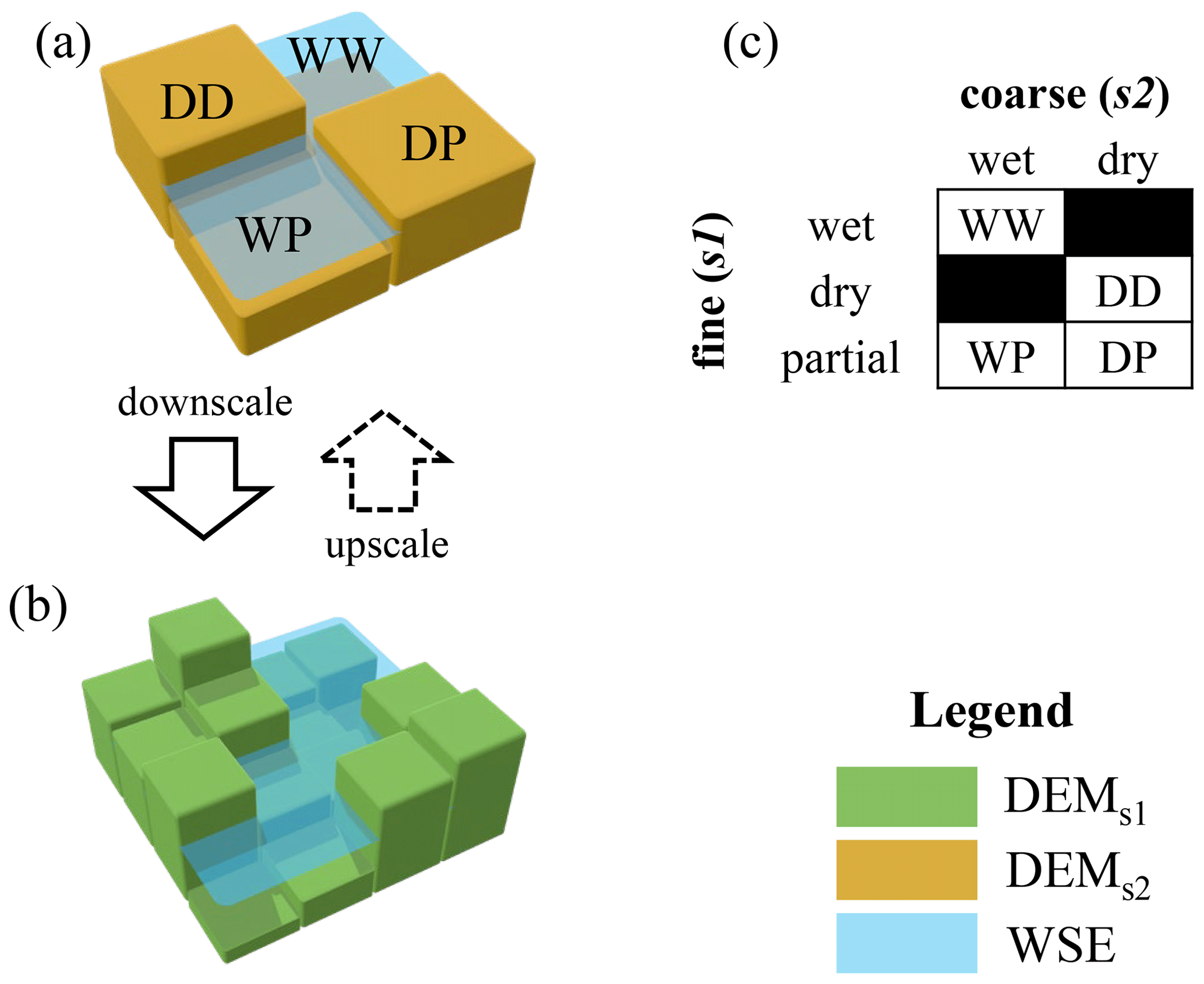
Figure 1Framework for classification of flood hazard resample case. Panel (a) shows conceptual coarse grids and the corresponding resample case calculated from Eq. (1). Panel (b) shows the corresponding fine grids, while panel (c) shows the case label acronyms. D, W, and P stand for dry, wet, and partial, respectively.
While downscaling flood grids is used by many global hazard models, to our knowledge only one study has addressed 2D downscaling of hydrodynamic model results (Schumann et al., 2014), and no studies have provided a comparison of methods. Addressing this, our objectives are twofold: (1) present our newly developed downscaling approach and (2) evaluate and compare our new approach to the state-of-the-art downscaling approach of Schumann et al. (2014) and two simple algorithms using a data-rich case study.
To better communicate and understand the challenges and solutions to rescaling flood hazard grids, we adapt the “resample case framework” from Bryant et al. (2023) to classify each cell in the s2 domain into one of four cases with similar disaggregation behaviour. Each case is defined by comparing the local coarse water depth value (WSHs2,j) to the corresponding fine values (WSHs1,i), where cell j is composed of a block of i cells as shown graphically in Fig. 1 and defined explicitly below:
where the first part of the casej label code is determined by the coarse cell (WSHs2), and the second letter is determined by the extremes of the fine cells (WSHs1). The quadrants in Fig. 1b provide a simple example of four such groups whose corresponding case labels are shown in panel (a). Because domain resample case classification is dependent on both input and output grids, classification is not directly used in any downscaling algorithms – instead, we use the framework to communicate the process and challenges of downscaling flood hazard grids.
Beginning with the simplest case, dry-dry (DD) zones are trivial and can be ignored for flood hazard rescaling operations as they remain unaltered: dry before and after rescaling (i.e., WSH=0). Wet-wet (WW) zones are also relatively simple as the group of WSEi cells should be roughly equivalent to their parent WSEj cell, an easy task for classic grid resampling tools like bilinear resampling. Wet-partial (WP) zones can be similarly obtained but with the additional step of removing dry s1 cells with an exceedance mask (i.e., cells where WSEs1<DEMs1 are set to null). Most difficult is the treatment of dry-partial (DP) zones which require some propagation or searching beyond the original coarse (s2) inundation footprint. In fact, this propagation challenge is a similar problem to that of a classic 2D hydrodynamic model; however, downscaling must employ simplifying assumptions to maintain advantageous computation times. This requires more sophisticated algorithms to propagate wet cells laterally like horizontal projection. Such horizontal projection may introduce artefacts like isolated flooding where disconnected groups of cells in low-lying terrain are shown as flooded (e.g., behind levees). Because high-resolution hydrodynamic models generally employ cell-connected routines, this isolated flooding can be considered erroneous within the paradigm of hydrodynamic downscaling. However, this paradigm can be a poor representation of actual flood behaviour in areas with high groundwater connectivity or imperfect flood defences. In summary, the downscaling problem can be broken into three zones: the first two (WW and WP) are relatively simple and, while some alternate approaches are possible, we do not expect large differences in performance in these zones. The final dry-partial (DP) zone is more challenging, and we therefore expect differences in treatment and performance between algorithms in this zone.
To validate and compare the novel resolution enhancement or downscaling algorithm, we first compute the requisite coarse-resolution (s2=32 m) input grid (WSEs2) using a calibrated hydrodynamic model. Using this input grid (WSEs2) and a fine-resolution terrain layer (DEMs1), we apply the novel downscaling algorithm to compute a fine-resolution enhanced grid (WSEs1=4 m). Using the same inputs, we then compute similar enhanced grids for the state-of-the-art downscaling algorithm from Schumann et al. (2014) and two simple algorithms representing solutions of minimum complexity. These enhanced grids (WSEs1), along with results from a calibrated fine-resolution hydrodynamic model (s1=4 m), are then evaluated against the maximum inundation extents and high water marks observed during a 2021 flood in Germany to validate and demonstrate the performance improvements of the novel algorithm.
3.1 Novel CostGrow algorithm
The novel “CostGrow” algorithm employs the four phases summarized in Fig. 2: (1) grid resampling, (2) least-cost mapping, (3) filtering high-and-dry sub-grid cells, and finally (4) an isolated-cell filter, all of which are parameterless. In the first grid resampling phase, various techniques have been developed by others for applications in image analysis and spatial analysis (Bierkens et al., 2000), with bilinear being the most common for terrain manipulations in hydraulic applications (Heritage et al., 2009; Muthusamy et al., 2021) as it provides a smooth result while preserving centroid values. For downscaling, bilinear resampling computes the s1 value from the four adjacent s2 centroid values weighted by distance as seen in Fig. 2a (notice the s2 values are preserved by the centre s1 cell). CostGrow implements bilinear resampling from the popular spatial analysis package GDAL (GDAL/OGR contributors, 2022). In the second phase, the resampled grid is extrapolated using a cost-distance analysis, a common GIS (geographic information system) algorithm for computing the path of least cost, determined by weighting distance and some cost map to obtain the effective distance from source cells to sink cells (Foltête et al., 2008). For this study, CostGrow implements a cost-distance routine with N8(P) adjacency and a neutral cost surface (Lindsay, 2014, CostAllocation). This first maps the dry portion of the domain in terms of catchment areas for each boundary cell WSEs1,i from the previous phase and then maps the corresponding boundary WSEs1,i cell value to each of its catchments. In effect, this grows or horizontally projects each WSEs1,i boundary cell value outwards, filling the dry domain with the WSEs1,i values that are closest in distance. For the toy example shown in Fig. 2b, this is a simple extrapolation onto the dry right-hand side of the domain. Future implementations could employ a non-neutral cost surface to incorporate levees or some other flood obstructions into the analysis. In the third phase, high-and-dry cells are filtered from this cost-distance map by comparing cell-by-cell to the terrain values (where ) as shown by the blank cells in Fig. 2c. This often results in many isolated pockets of flooding in low-lying areas shown beyond the initial contiguous WSEs2 flood (see Fig. 2c red circle). In the final phase, these isolated or disconnected groups of flooded cells are filtered from the result such that only the largest or main flooded water body remains. To accomplish this, the filtered grid is converted to a binary inundation grid, from which each contiguous clump is identified and ranked according to size (See “Clump” tool from Lindsay, 2014) (see Fig. 2d). From the largest clump, an inverted mask is generated and applied to the water level grid to remove isolated flooding cells from the result.
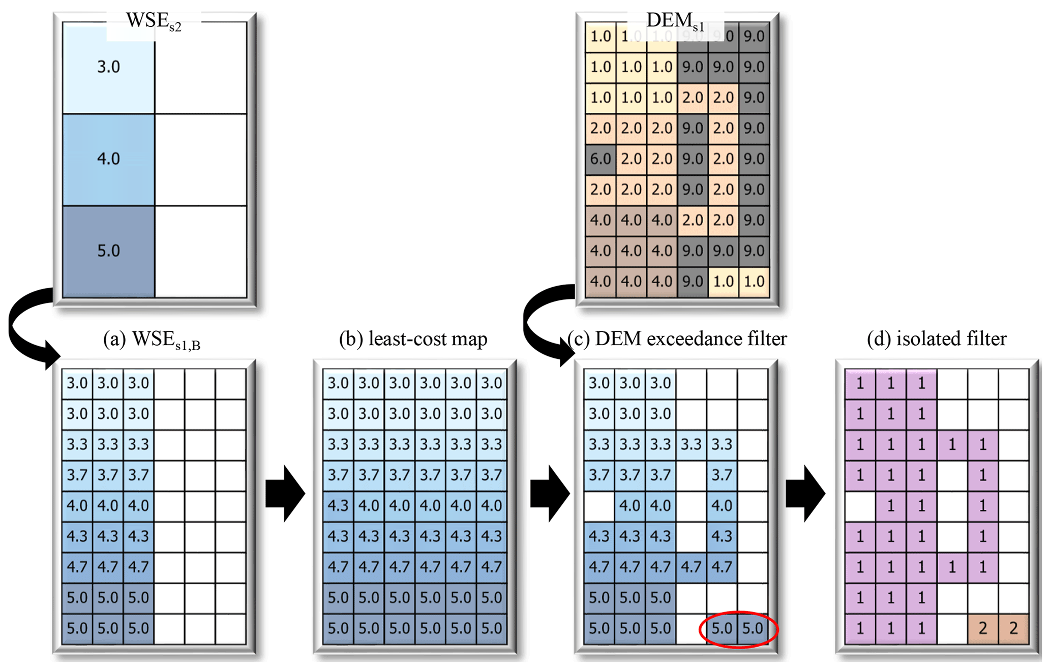
Figure 2Toy example of the novel CostGrow downscaling algorithm showing WSE, DEM, and clump analysis grids for the four phases: (a) bilinear resampling of coarse water level WSEs2 grid; (b) extrapolation using least-cost mapping from WSEs1,B values; (c) application of DEM exceedance mask to filter high-and-dry cells; and (d) results of clump analysis, from which the isolated mask is generated to filter all but the largest group (1 in this case). See the main text for details.
3.2 Validation and comparison
3.2.1 Case study, data, and hydrodynamic modelling
To evaluate the aforementioned downscaling algorithms, data obtained from the July 2021 flooding of the Ahr river in Germany are used. This was the most extreme flood event to hit the region in living memory, with precipitation exceeding a 500-year return period (Dietze et al., 2022), a difficult-to-estimate peak discharge (Vorogushyn et al., 2022), and 134 casualties in the Ahr valley (Szönyi and Roezer, 2022). The data used for this study are summarized in Table 1 and Fig. 3.
Brell et al. (2023)Apel et al. (2022)Apel et al. (2022)OpenStreetMap contributors (2022)Landesamt für Umwelt Rheinland-Pfalz (2022)Copernicus Land Monitoring Service (2018)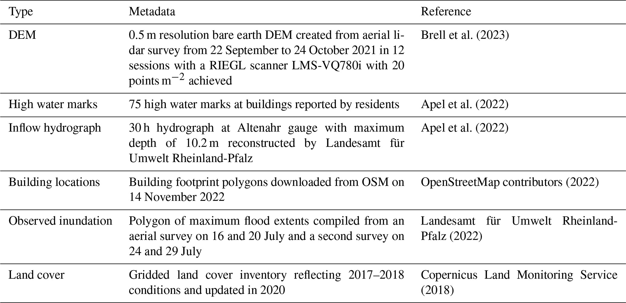
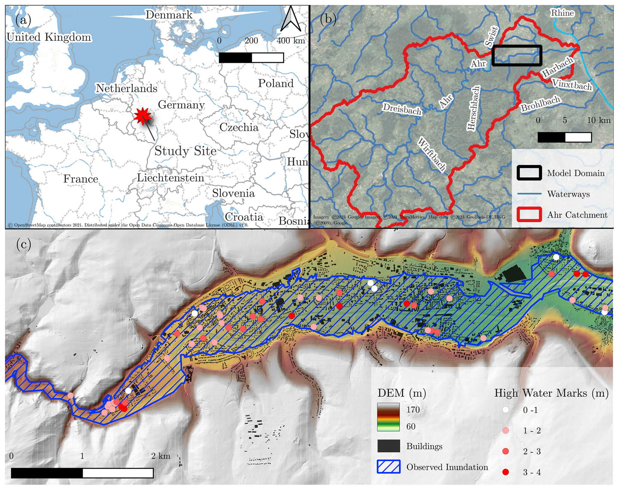
Figure 3Study site maps showing (a) location map, (b) Ahr catchment map, and (c) downscaling domain with main datasets (see Table 1 for descriptions).
To construct the coarse water grid for use as an input in downscaling (WSEs2) and a second grid for validation and comparison (WSEs1), coarse- (s2=32 m) and fine-resolution (s1=4 m) twin hydrodynamic models are calibrated to the observed inundation extents using the critical success index. The hydrodynamic models are constructed in the 2D raster-based RIM2D framework (Apel, 2023) and run on a Tesla P100 GPU. RIM2D implements a simplified version of the shallow-water equations after Bates et al. (2010). A reconstructed hydrograph is used for the upstream boundary condition, and other model parameters are described in Apel et al. (2022). The model terrain is generated through bilinear resampling of the bare earth DEM (Table 1) to the target resolution. For the treatment of urban areas, blocking out buildings has been shown to be a more accurate way to represent buildings within a relatively high-resolution hydrodynamic model (Bellos and Tsakiris, 2015). In coarse models however, especially where the building size (and space between) is smaller than a grid cell, blocking-out reduces model performance, especially in and around buildings. Regardless, blocking-out could be included in a downscaling algorithm (and the high-resolution validation model); however, as this requires a more complicated algorithm and is not included in the current state-of-the-art methods against which we compare, we opted to avoid blocking-out and instead apply a separate roughness coefficient to built-up areas in both models (and all downscaling algorithms) to capture the blocking effects of buildings (a.k.a. the “urban porosity approach”).
To obtain accurate maximum WSE grids from the twin hydrodynamic models, a calibration routine is used to optimize model roughness using the critical success index (CSI) (see Table S2 for definition) of the maximum simulated inundation calculated against the observed inundation from Table 1. Two unique Manning's roughness values (built-up and channel/floodplain) are treated as free parameters for each model and optimized while a third roughness value for forested areas is held fixed (), as Apel et al. (2022) showed this third region to have negligible influence. The three roughness values are spatially allocated according to land cover (Table 1) as described in Apel et al. (2022). Finally, the optimal roughness values are obtained using a mix of trial and error and the Newton–conjugate-gradient algorithm (Nocedal and Wright, 2006; Virtanen et al., 2020) to optimize the critical success index (CSI).
The best performing effective roughness values for the twin hydrodynamic models s2=32 m and s1=4 m are 0.867 and 0.175 for urban areas and 0.089 and 0.133 for channel areas with a CSI of 0.885 and 0.914, respectively, as shown in Figs. S1 and S2. These counter-intuitive relative roughnesses are a result of differences in floodplain–channel dynamics necessary to match the observed inundation footprint between the two models. In the coarse hydrodynamic model, the river channel is poorly represented by the 32 m resolution which is roughly 3 times larger than the channel. Thus, the flow in the channel and the channel-floodplain interactions show different dynamics compared to the more realistic fine-resolution model. The calibration routine compensates for these differences with the disproportionate roughness values reported above. However, as our focus is on downscaling performance, the less-accurate representation of channel dynamics and water levels (as opposed to inundation extents) provided by the coarse model are inconsequential considering we apply the fine and coarse hydrodynamic model results comparatively in all scenarios. Additional figures, performance measures, and discussion for the calibration are provided in the Supplement. To remove any boundary effects, the hydrodynamic model results are cropped to a smaller domain for the downscaling analysis (13.4×6.6 km to 8.9×3.5 km; see Fig. S3).
3.2.2 Downscaling algorithms for comparison
To demonstrate the performance of the novel CostGrow algorithm relative to similar algorithms, two simple algorithms representing solutions of minimum complexity and the state of the art from Schumann et al. (2014) are described below and included in the comparison.
The first simple algorithm considered here is a bilinear grid resampling (see “Resample” in Fig. 4c), which is identical to the above-described first phase of the novel CostGrow algorithm. This algorithm is the only one considered that does not make use of the fine-resolution terrain values (DEMs1) and therefore carries an obvious limitation in wet-partial (WP) regions, where sub-grid high-and-dry ground elevations may be present within a wet coarse cell (see red circle in Fig. 4a). To address this, the second simple algorithm we consider (see “TerrainFilter” in Fig. 4d) builds and applies a terrain exceedance mask (WSEs2<DEMs2) which removes those cells where depths are negative from the resulting WSEs1. Neither of these simple algorithms treat cells outside the wet coarse domain (i.e., the dry-partial (DP) zone remains dry).
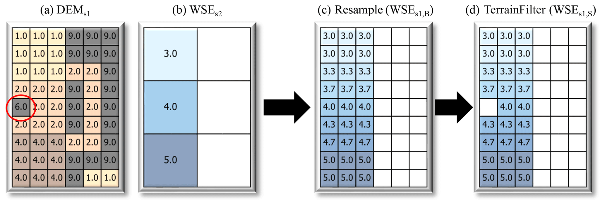
Figure 4Toy example of simple flood downscaling inputs and algorithms showing the following: (a) input fine-resolution terrain grid, (b) input coarse-resolution water level grid, (c) “Resample” downscaling result, and (d) “TerrainFilter” downscaling result described in the text.
To the best of our knowledge, the method by Schumann et al. (2014) (denoted “Schumann14”) is the state of the art in 2D flood grid downscaling algorithms. This algorithm was developed to downscale 1D/2D hybrid inundation model results from 600 to 30 m by employing a two-tier approach: first, the 1D channel regions are downscaled assuming a water surface plane between sections; second, 2D floodplain regions are downscaled using a nearest-neighbour search. For our study, we focus on the floodplain portion of the algorithm for which the source code was provided to the study team and which has roughly the three steps shown in Fig. 5. First, a search zone is built using a buffer of width that is one half the coarse resolution around all wet cells in the coarse domain (i.e., wet-partial (WP) and wet-wet (WW) regions). An alternate buffer distance parameter is possible, but here we select the same parameter value as Schumann et al. (2014). Second, within the search zone, each fine (s1) cell searches for the nearest coarse (s2) cell using a nearest-neighbour city-block (also called “Manhattan”) search algorithm which replicates the same N4(P) adjacency used by their inundation model. Finally, the WSEs1 nearest-neighbour search result is combined with a simple grid resample (also using nearest-neighbour), and a terrain exceedance mask is applied. While this algorithm improves upon the simple approaches, the blocky WSEs2 values remain in the fine WSEs1 result, isolated flooding artefacts are introduced (red circle in Fig. 5d), and the per-cell nearest-neighbour search is computationally expensive. Finally, the algorithm was originally written in the MATLAB programming language and was not made public or widely shared.
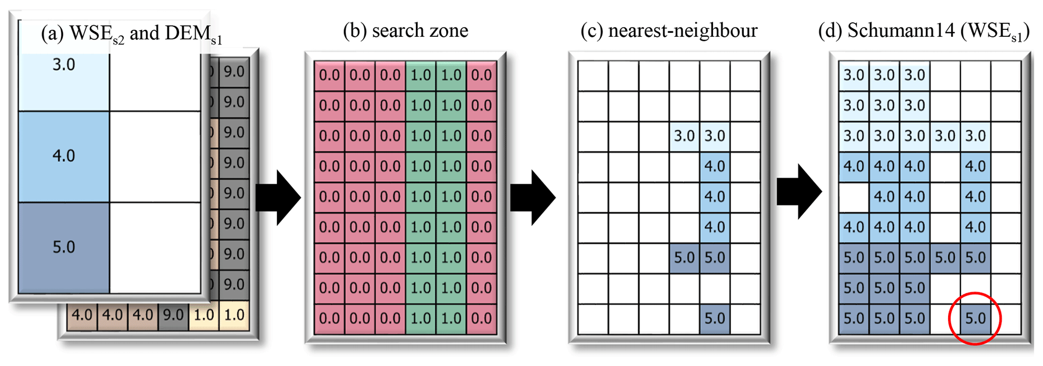
Figure 5Toy example of a floodplain downscaling algorithm by Schumann et al. (2014) showing the following: (a) input fine-resolution terrain grid and coarse-resolution water level grid (see Fig. 4a), (b) search zone, (c) nearest-neighbour search result, and (d) WSEs1 downscaling result. See the main text for details.
Compared to the above Schumann14 algorithm, we expect three main advantages from the novel CostGrow algorithm. First, CostGrow should be substantially more computationally efficient by avoiding the cell-by-cell nearest-neighbour search. Second, CostGrow should be slightly more accurate in reproducing fine-resolution inundation extents by avoiding the fixed search radius and including an isolated flooding filter. Third, the accuracy of water levels should improve due to the incorporation of the aforementioned inundation extent mechanisms in dry-partial regions and the replacement of the initial nearest-neighbour resampling with bilinear resampling. These expectations are tested below using a case study. Table 2 provides a brief summary of all the downscaling algorithms considered by this study and the two hydrodynamic models used.
Schumann et al. (2014)Table 2Downscaling algorithms and hydrodynamic models included in this evaluation showing resample casej applicability (see Fig. 1) and case study runtime to achieve output grids (WSEs1=4 m for all except Hydro. (s2) which outputs WSEs2=32 m).
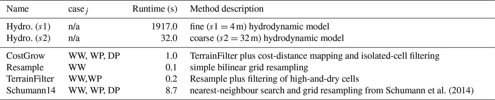
n/a: not applicable.
Water level grids obtained from the twin calibrated hydrodynamic models and the four downscaling algorithms as well as their corresponding inundation performances are shown in Fig. 6. For the models, Fig. 6a4 and b4 show the fine (s1) parameterization, while the results for the Resample downscaling algorithm (Fig. 6a0 and b0) show the performance of the coarse (s2) parameterization (because this algorithm does not alter the coarse extents). This suggests both parameterizations reproduce the observed inundation well, with the fine (s1) obtaining a slightly better CSI as expected considering the complex topography. The coarse (s2) model converged on lower water levels and extents to obtain the optimal CSI, as shown by the lower error bias (0.205 vs. 1.029) and the calibration contour plots (Figs. S1 and S2).
Figure 6 suggests that there are some discrepancies between the observed inundation, which has a single contiguous inundation extent without holes, and the DEM, which contains some micro-topography that likely would have remained dry during the flood (see Fig. 8, point A), suggesting that the observed inundation is slightly conservative (i.e., overestimates the true flood extents). These discrepancies may be attributable to the methods used by Landesamt für Umwelt Rheinland-Pfalz (2022) to map the extents or the earthworks undertaken between the inundation mapping surveys (late July) and the lidar survey (October). Regardless, these discrepancies are relatively minor, and we consider them negligible for our research objective of evaluating the CostGrow algorithm.
Comparing the inundation performance of the downscaling algorithms in general, the more complex algorithms performed better, with the novel CostGrow and Schumann14 algorithms performing similarly. Specifically, the four common inundation performance metrics in Fig. 6, panels b0–b3, show that CostGrow and Schumann14 have nearly identical performances, with all metrics (with one exception) outperforming the simple algorithms Resample and TerrainFilter. The exception is that TerrainFilter has the lowest false alarm rate (0.014), an artefact which can be explained by two concurrent hypothesis: (1) the TerrainFilter algorithm does not address dry-partial (DP) regions but does filter wet-partial (WP) regions, giving it the smallest inundation area and making it the least likely to overestimate inundation, and (2) the overestimation bias in the observed inundation discussed earlier favours methods that underestimate.
The inundation metrics reported in Fig. 6 are sensitive to both the hydraulic character of the study region and the particular domain selected for analysis; for example, we expect a broad, flat floodplain or different boundary conditions to yield different metric values. For the results reported here, we selected the domain 8.9×3.5 km by balancing hydraulic continuity and controlling for boundary effects and computational cost; however, other similar domains were tested during the study preparation, and the relative ranking of performance between the downscaling algorithms was found to be consistent, with CostGrow outperforming Schumann14 slightly for some domains. For example, the CSI of the detailed area (Fig. 6, blue box) is 0.813 for CostGrow and 0.811 for Schumann14. This aligns with our expectation that CostGrow's inundation results would slightly outperform that of Schumann14 given the absence of a fixed search radius and use of an isolated filter in the CostGrow algorithm. Regardless, this evaluation suggests that, while gains in computation performance are substantial, gains in standard qualitative inundation performance over Schumann14 are negligible. Qualitatively however, CostGrow generates more physically coherent depth grids in some fringe areas as shown in Figs. 8 and S4.
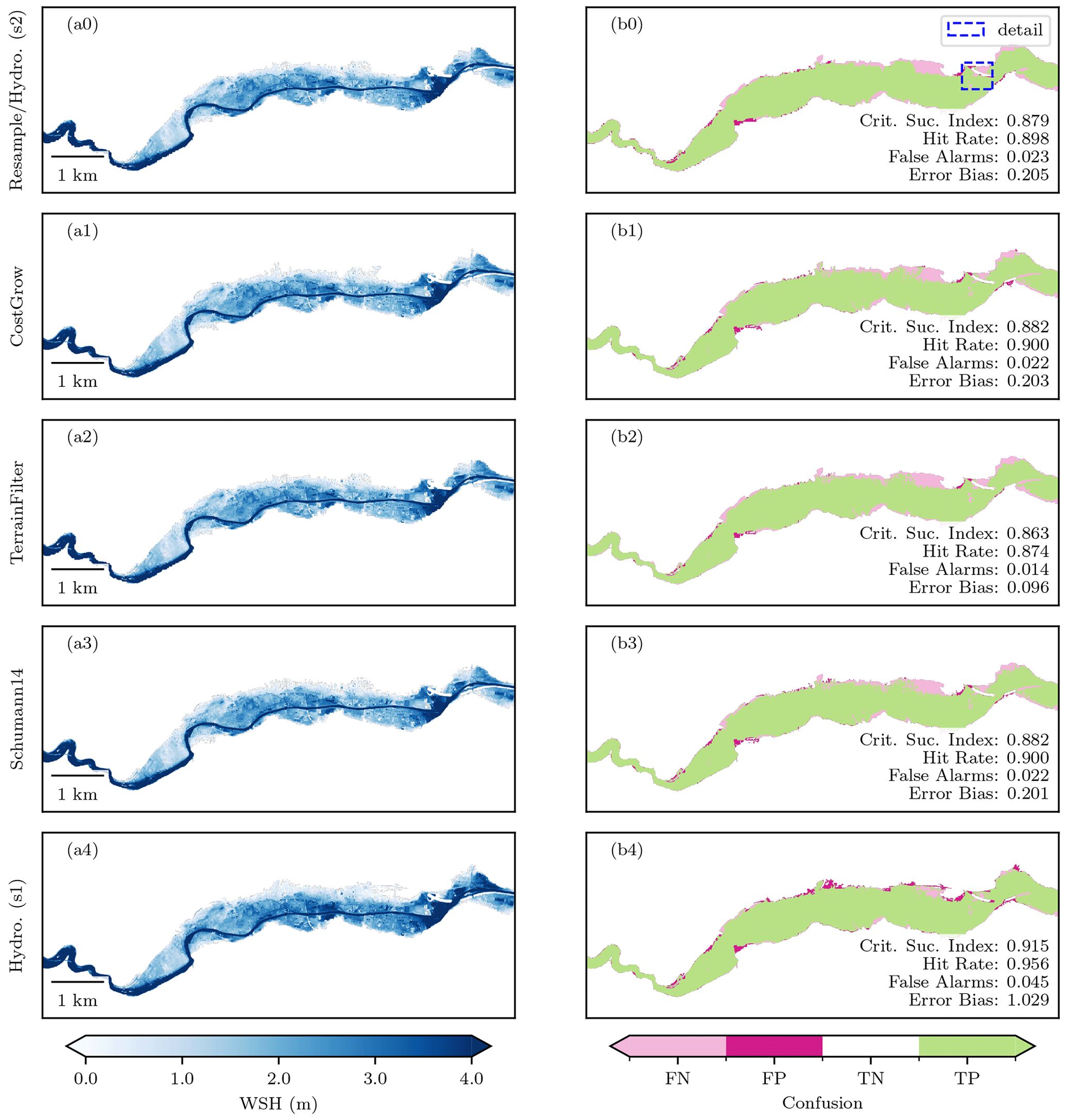
Figure 6Downscaled and hydrodynamic model WSHs1 results and corresponding inundation performance. Left-hand side panels (a) show the water depth grids (WSHs1) obtained from the coarse and fine hydrodynamic model (a0 and a4) and the four downscaling algorithms (a0–a3; see Table 2 and main text for description). Similarly, the right-hand side panels (b) show the domain inundation classification confusion map (false negative (FN), false positive (FP), true negative (TN), and true positive (TP) cells – see Table S1) and the common inundation performance metrics defined in Table S2. The Resample algorithm and coarse hydrodynamic model results (s2) are identical and therefore shown as one panel. See Fig. 8 for the detailed area.
Examining the water level performance of the hydrodynamic models, Fig. 7 shows that the coarse (s2=32 m; panel a0) and fine (s1=4 m; panel c1) models reproduce the observations well. This is remarkable considering the models were calibrated on inundation extents (using CSI), not water levels, and that the water levels are reported by residents. Similar to inundation performance, Fig. 7 also shows that the fine model (s1=4 m) performs best, while the coarse model (s2=32 m) slightly underestimates (see Fig. S3 for a map of WSE differences between s2=32 m and s1=4 m). Figure 7 also shows that, like for inundation performance, CostGrow and Schumann14 have better performances than the simple algorithms and the coarse hydrodynamic model; however, the performance of CostGrow slightly surpasses that of Schumann14. Given the more comparable inundation performance, we conclude that the advantage seen here emerges from CostGrow's application of bilinear resampling as opposed to Schumann14's nearest-neighbour resampling; however, owing to the relatively small scale ratios (4:32), this advantage is minor. Comparing the simple algorithms in Fig. 7 (panels c0 and a1) shows that the treatment of wet-partial regions provides no improvement in reproducing high water marks, unlike the advantages seen for inundation performance. We hypothesize that this is due to the absence of any high-water-mark observations on dry cells in wet-partial regions. In other words, TerrainFilter only improves the filtering of false positives when compared to the Resample result, and false positive regions can not be evaluated by high-water-mark observations (as these regions are dry in reality).
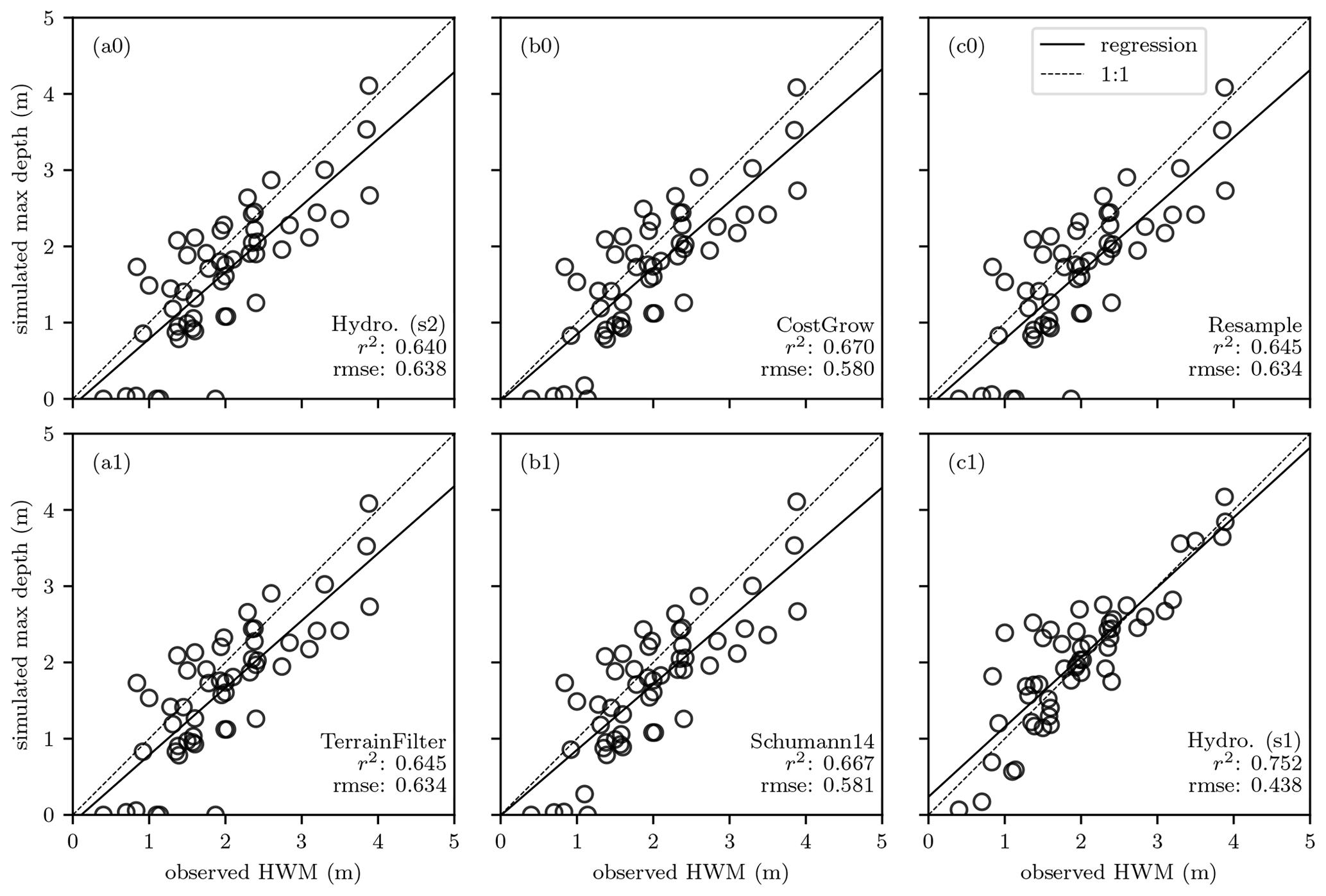
Figure 7Linear correlation between July 2021 resident-reported high water marks (see Table 1) and maximum simulated depth of twin hydrodynamic models (a0, c1) and downscaling algorithms (b0, c0, a1, b1).
Focusing on a small region, Fig. 8 shows a portion of the domain where floodwaters likely flowed behind a highway embankment along a small frontage road travelling underneath an overpass (point E). Because the observed inundation layer was mapped primarily by air (Landesamt für Umwelt Rheinland-Pfalz, 2022), these observation data show the area underneath the overpass as dry; therefore, any simulated inundation in this area is marked as false positive (FP) – supporting our hypothesis that the observed inundation is slightly conservative. Other performance and behavioural differences between the algorithms can also be seen in this area: the lack of treatment for wet-partial regions (point A) and dry-partial regions (point B) in the simple algorithms, how CostGrow is not limited to a search radius like Schumann14 for dry-partial treatment (point C), the isolated inundation artefacts in Schumann14 (point D), and the blocky result of Schumann14's nearest-neighbour resampling in wet-wet (WW) and wet-partial (WP) regions (panel b1).
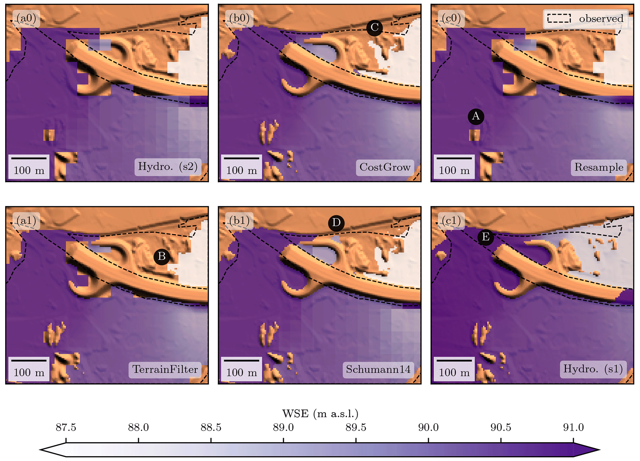
Figure 8Downscale and hydrodynamic model WSE detailed results. Observed inundation is shown in black for reference. See Fig. 6b0 for location and the main text for a description.
Runtimes for the twin hydrodynamic models and the four downscaling algorithms are shown in Table 2. As expected, the algorithms of higher complexity also have higher runtimes, and all downscaling algorithms are substantially faster than the hydrodynamic models (which simulate a flood wave of 833 min). Despite minimal effort being invested in optimization, the novel CostGrow algorithm is substantially faster than the state-of-the-art algorithm from Schumann et al. (2014). These runtimes may be improved through parallelization and other programming improvements. Regardless, because the algorithm by Schumann et al. (2014) employs a cell-by-cell nearest-neighbour search, it is fundamentally less efficient than those like CostGrow which employ least-cost mapping.
Comparing alternate approaches to obtain fine-resolution flood grids (4 m in this case), the total runtime of a pipeline implementing the CostGrow downscaling algorithm (on top of the coarse hydrodynamic model) was roughly 33 s versus the 34 min necessary for our 4 m native hydrodynamic model, a 60-fold improvement. This reduced runtime has a corresponding loss in temporal resolution (only the maximum WSE is downscaled) and inundation accuracy of 0.03 CSI and high-water-mark accuracy of 0.14 RMSE when comparing the CostGrow downscaling algorithm pipeline to the 4 m native hydrodynamic model for our study. Were a slower hydrodynamic model used (e.g., a non GPU-parallelized platform) or a larger downscaling ratio (32:4 in our case), the efficiency gain of downscaling over fine hydrodynamic modelling would increase, while shortening the simulation time (833 min in our case) would reduce the efficiency gain. For example, during study development we implemented similar twin hydrodynamic models in the LISFLOOD-FP 8.1 framework using a second-order discontinuous Galerkin solver which implements the full shallow-water equations (Shaw et al., 2021). Executed on eight CPU cores, the runtimes for these models was 7100.00 and 0.43 min for the 4 and 32 m discretization respectively – were a CostGrow downscaling algorithm pipeline implemented with this setup, we estimate a 16 000-fold improvement in runtime to obtain a comparable WSEs1=4 m grid.
The flood grid downscaling algorithms presented here make estimates based on simple hydraulic assumptions and the DEM. Because of this, these algorithms do not consider sub-grid or other hydraulically relevant elements not contained in the DEM like levees, flood walls, or storm drainage systems. The significance of this limitation will depend on the particular case, but any study where levees or barriers are present but not resolved by the DEM should be treated with extra caution when employing downscaling. Much like hydrodynamic models, sub-grid obstructions like levees could be incorporated into downscaling algorithms, e.g., using a non-neutral cost surface in CostGrow's cost-distance routine.
Future work should explore evaluation techniques for flood-related algorithms, where the techniques are less sensitive to study area, domain size, hardware, and software of a particular study. For example, a collection of fully-open data-rich flood events with a wide range of hydraulic character would facilitate more meaningful comparisons of model or algorithm performance across platforms and between researchers. Further, such additional case studies with varied hydraulic character would help to quantify and communicate the benefits and limitations of downscaling in different hydraulic regimes. To better support the emerging needs of impact forecasting, where 2D velocity grids are sometimes desired, pursuing a method that is also capable of downscaling velocity could be of use; however, this would require blocking out buildings in the hydrodynamic model. Further performance enhancements of downscaling methods may be found by incorporating machine learning techniques originally developed for image enhancement which have recently been applied to enhance terrain models (Demiray et al., 2021).
This study has developed, demonstrated, and evaluated the novel CostGrow algorithm for resolution enhancement or downscaling of floodwater surface grids. This algorithm outperforms the state of the art, with a sixfold improvement in runtime for our case study, a slight improvement in standard performance metrics, and improvements in some fringe areas using qualitative evaluation. When compared to results obtained through fine-resolution hydrodynamic modelling, the proposed downscaling algorithm (in conjunction with coarse-resolution modelling) showed a 60-fold improvement in runtimes with a slight loss of accuracy.
In general, coarse modelling in conjunction with downscaling is shown to be an effective means of obtaining fine-resolution inundation grids at a fraction of the computational cost. However, the utility of employing downscaling to obtain fine-resolution grids is limited by the availability and quality of fine-resolution DEMs. A potential application of downscaling is to facilitate the post-processing of fine-resolution inundation result layers from global models for data-rich regions where a local fine-resolution DEM is available. This could be a cost-effective way to deliver fine-resolution inundation maps to any region on the globe without the need for specialized modelling expertise or resources. Regardless, the lack of attention to the subject of downscaling in the academic literature suggests some space remains for downscaling to improve the efficiency of model chains. Towards this, the downscaling algorithms developed in this study have been made open source and are available as QGIS processing scripts (https://github.com/cefect/FloodRescaler, last access: 1 February 2024).
Scripts used in downscaling analysis and figure production are provided by Bryant (2024, https://doi.org/10.5281/zenodo.10607407). For a more usable Python package, see the FloodDownscaler2 project (https://github.com/cefect/FloodDownscaler2, last access: 1 February 2024) (not used for this publication). Easy-to-use QGIS processing scripts (not used for this publication) are provided in the FloodRescaler project (https://github.com/cefect/FloodRescaler, last access: 1 February 2024).
Case study data used to construct the hydrodynamic models and perform the validation are summarized in Table 1 and the corresponding references (all data except the high water marks are public). Grids used in the downscaling analysis are available upon request.
The supplement related to this article is available online at: https://doi.org/10.5194/hess-28-575-2024-supplement.
SB developed the concept, analysis, and writing with contributions from other co-authors. SB developed the software, formal analysis, and investigation. GS provided the MATLAB source code for the Schumann14 algorithm. HA requested and managed the calibration data and provided early versions of the hydrodynamic models. BM and HK supervised the work.
The contact author has declared that none of the authors has any competing interests.
Publisher’s note: Copernicus Publications remains neutral with regard to jurisdictional claims made in the text, published maps, institutional affiliations, or any other geographical representation in this paper. While Copernicus Publications makes every effort to include appropriate place names, the final responsibility lies with the authors.
The research presented in this article was conducted within the research training group “Natural Hazards and Risks in a Changing World” (NatRiskChange) funded by the Deutsche Forschungsgemeinschaft (DFG; GRK 2043/2). We are thankful to Oliver Wing for his insightful conversations on the topic, Jeff Neal for help with early attempts to implement LISFLOOD-FP, Knut Günther for keeping the section running, Karen Lebek for her brilliant coordination, and the whole NatRiskChange community for support and friendship. And I am particularly indebted to my wife Jody for watching baby Tarn so I could finish this manuscript.
This paper was edited by Alberto Guadagnini and reviewed by two anonymous referees.
Aires, F., Miolane, L., Prigent, C., Pham, B., Fluet-Chouinard, E., Lehner, B., and Papa, F.: A Global Dynamic Long-Term Inundation Extent Dataset at High Spatial Resolution Derived through Downscaling of Satellite Observations, J. Hydrometeorol., 18, 1305–1325, https://doi.org/10.1175/JHM-D-16-0155.1, 2017. a
Alipour, A., Jafarzadegan, K., and Moradkhani, H.: Global sensitivity analysis in hydrodynamic modeling and flood inundation mapping, Environ. Modell. Softw., 152, 105398, https://doi.org/10.1016/j.envsoft.2022.105398, 2022. a
Apel, H.: hydro / rfm / RIM2D, https://git.gfz-potsdam.de/hydro/rfm/rim2d (last access: 1 February 2024), 2023. a
Apel, H., Vorogushyn, S., and Merz, B.: Brief communication: Impact forecasting could substantially improve the emergency management of deadly floods: case study July 2021 floods in Germany, Nat. Hazards Earth Syst. Sci., 22, 3005–3014, https://doi.org/10.5194/nhess-22-3005-2022, 2022. a, b, c, d, e
Banks, J. C., Camp, J. V., and Abkowitz, M. D.: Scale and Resolution Considerations in the Application of HAZUS-MH 2.1 to Flood Risk Assessments, Nat. Hazards Rev, 16, 04014025, https://doi.org/10.1061/(ASCE)NH.1527-6996.0000160, 2015. a
Bates, P. D., Horritt, M. S., and Fewtrell, T. J.: A simple inertial formulation of the shallow water equations for efficient two-dimensional flood inundation modelling, J. Hydrol., 387, 33–45, https://doi.org/10.1016/j.jhydrol.2010.03.027, 2010. a
Bates, P. D., Quinn, N., Sampson, C., Smith, A., Wing, O., Sosa, J., Savage, J., Olcese, G., Neal, J., Schumann, G., Giustarini, L., Coxon, G., Porter, J. R., Amodeo, M. F., Chu, Z., Lewis‐Gruss, S., Freeman, N. B., Houser, T., Delgado, M., Hamidi, A., Bolliger, I., McCusker, K., Emanuel, K., Ferreira, C. M., Khalid, A., Haigh, I. D., Couasnon, A., Kopp, R., Hsiang, S., and Krajewski, W. F.: Combined Modeling of US Fluvial, Pluvial, and Coastal Flood Hazard Under Current and Future Climates, Water Resour. Res., 57, https://doi.org/10.1029/2020WR028673, 2021. a
Bellos, V. and Tsakiris, G.: Comparing Various Methods of Building Representation for 2D Flood Modelling In Built-Up Areas, Water Resour. Manag., 29, 379–397, https://doi.org/10.1007/s11269-014-0702-3, 2015. a
Bierkens, M., Finke, P., and De Willigen, P.: Upscaling and downscaling methods for environmental research, Kluwer Academic, ISBN 0-7923-6339-6, 2000. a
Brell, M., Roessner, S., Dietze, M., Bell, R., Magnussen, S., Schreck, D., Jany, S., Ozturk, U., Merz, B., and Thieken, A.: Eifel Flood 2021–Airborne Laser Scanning (ALS) and Orthophoto Data, https://doi.org/10.5880/GFZ.1.4.2023.003, 2023. a
Bryant, S.: cefect/FloodDownscaler: HESS final (v2024-02-01), Zenodo [code], https://doi.org/10.5281/zenodo.10607407, 2024. a
Bryant, S., Kreibich, H., and Merz, B.: Bias in Flood Hazard Grid Aggregation, Water Resour. Res., 59, e2023WR035100, https://doi.org/10.1029/2023WR035100, 2023. a
Copernicus Land Monitoring Service: European Union, Copernicus Land Monitoring Service 2018, European Environment Agency (EEA), https://land.copernicus.eu/pan-european/corine-land-cover (last access: 1 February 2024), 2018. a
de Moel, H., van Alphen, J., and Aerts, J. C. J. H.: Flood maps in Europe – methods, availability and use, Nat. Hazards Earth Syst. Sci., 9, 289–301, https://doi.org/10.5194/nhess-9-289-2009, 2009. a
Demiray, B. Z., Sit, M., and Demir, I.: D-SRGAN: DEM Super-Resolution with Generative Adversarial Networks, SN Computer Science, 2, 48, https://doi.org/10.1007/s42979-020-00442-2, 2021. a
Dietze, M., Bell, R., Ozturk, U., Cook, K. L., Andermann, C., Beer, A. R., Damm, B., Lucia, A., Fauer, F. S., Nissen, K. M., Sieg, T., and Thieken, A. H.: More than heavy rain turning into fast-flowing water – a landscape perspective on the 2021 Eifel floods, Nat. Hazards Earth Syst. Sci., 22, 1845–1856, https://doi.org/10.5194/nhess-22-1845-2022, 2022. a
Dong, C., Loy, C. C., He, K., and Tang, X.: Image Super-Resolution Using Deep Convolutional Networks, arXiv [preprint], http://arxiv.org/abs/1501.00092, arXiv:1501.00092 [cs] version: 3, 2015. a
Fewtrell, T. J., Bates, P. D., Horritt, M., and Hunter, N. M.: Evaluating the effect of scale in flood inundation modelling in urban environments, Hydrol. Process., 22, 5107–5118, https://doi.org/10.1002/hyp.7148, 2008. a
Fluet-Chouinard, E., Lehner, B., Rebelo, L.-M., Papa, F., and Hamilton, S. K.: Development of a global inundation map at high spatial resolution from topographic downscaling of coarse-scale remote sensing data, Remote Sens. Environ., 158, 348–361, https://doi.org/10.1016/j.rse.2014.10.015, 2015. a
Foltête, J., Berthier, K., and Cosson, J.: Cost distance defined by a topological function of landscape, Ecol. Model., 210, 104–114, https://doi.org/10.1016/j.ecolmodel.2007.07.014, 2008. a
Fraehr, N., Wang, Q. J., Wu, W., and Nathan, R.: Development of a Fast and Accurate Hybrid Model for Floodplain Inundation Simulations, Water Resour. Res., 59, e2022WR033836, https://doi.org/10.1029/2022WR033836, 2023. a
GDAL/OGR contributors: GDAL/OGR Geospatial Data Abstraction software Library, Open Source Geospatial Foundation, Zenodo [code], https://doi.org/10.5281/zenodo.5884351, 2022. a
Ghimire, E. and Sharma, S.: Flood Damage Assessment in HAZUS Using Various Resolution of Data and One-Dimensional and Two-Dimensional HEC-RAS Depth Grids, Nat. Hazards Rev, 22, 04020054, https://doi.org/10.1061/(ASCE)NH.1527-6996.0000430, 2021. a
Hall, J. W., Sayers, P. B., and Dawson, R. J.: National-scale Assessment of Current and Future Flood Risk in England and Wales, Nat. Hazards, 36, 147–164, https://doi.org/10.1007/s11069-004-4546-7, 2005. a
Heritage, G. L., Milan, D. J., Large, A. R., and Fuller, I. C.: Influence of survey strategy and interpolation model on DEM quality, Geomorphology, 112, 334–344, https://doi.org/10.1016/j.geomorph.2009.06.024, 2009. a
Horritt, M. S. and Bates, P. D.: Effects of spatial resolution on a raster based model of flood flow, J. Hydrol., 253, 239–249, https://doi.org/10.1016/S0022-1694(01)00490-5, 2001. a
Jongman, B., Kreibich, H., Apel, H., Barredo, J. I., Bates, P. D., Feyen, L., Gericke, A., Neal, J., Aerts, J. C. J. H., and Ward, P. J.: Comparative flood damage model assessment: towards a European approach, Nat. Hazards Earth Syst. Sci., 12, 3733–3752, https://doi.org/10.5194/nhess-12-3733-2012, 2012. a
Landesamt für Umwelt Rheinland-Pfalz: Hochwasser im Juli 2021, Tech. rep., Landesamt für Umwelt Rheinland-Pfalz, https://lfu.rlp.de/fileadmin/lfu/Wasserwirtschaft/Ahr-Katastrophe/Hochwasser_im_Juli2021.pdf (last access: 2 March 2023), 2022. a, b, c
Li, S., Sun, D., Goldberg, M., Kalluri, S., Sjoberg, B., Lindsey, D., Hoffman, J., DeWeese, M., Connelly, B., Mckee, P., and Lander, K.: A downscaling model for derivation of 3-D flood products from VIIRS imagery and SRTM/DEM, ISPRS J. Photogram., 192, 279–298, https://doi.org/10.1016/j.isprsjprs.2022.08.025, 2022. a
Lindsay, J.: The whitebox geospatial analysis tools project and open-access GIS, in: Proceedings of the GIS Research UK 22nd Annual Conference, The University of Glasgow, 16–18, https://jblindsay.github.io/ghrg/pubs/LindsayGISRUK2014.pdf (last access: 1 February 2024), 2014. a, b
Mohanty, M. P., Nithya, S., Nair, A. S., Indu, J., Ghosh, S., Mohan Bhatt, C., Srinivasa Rao, G., and Karmakar, S.: Sensitivity of various topographic data in flood management: Implications on inundation mapping over large data-scarce regions, J. Hydrol., 590, 125523, https://doi.org/10.1016/j.jhydrol.2020.125523, 2020. a
Muthusamy, M., Casado, M. R., Butler, D., and Leinster, P.: Understanding the effects of Digital Elevation Model resolution in urban fluvial flood modelling, J. Hydrol., 596, 126088, https://doi.org/10.1016/j.jhydrol.2021.126088, 2021. a, b, c, d
Nocedal, J. and Wright, S. J.: Numerical Optimization, Springer Series in Operations Research and Financial Engineering, Springer New York, ISBN 978-0-387-30303-1, https://doi.org/10.1007/978-0-387-40065-5, 2006. a
Nones, M. and Caviedes‐Voullième, D.: Computational advances and innovations in flood risk mapping, J. Flood Risk Manag., 13, e12666, https://doi.org/10.1111/jfr3.12666, 2020. a
OpenStreetMap contributors: Planet dump retrieved from https://planet.osm.org (last access: 14 November 2022), published: https://www.openstreetmap.org (last access: 1 February 2024), 2022. a
Papaioannou, G., Loukas, A., Vasiliades, L., and Aronica, G. T.: Flood inundation mapping sensitivity to riverine spatial resolution and modelling approach, Nat. Hazards, 83, 117–132, https://doi.org/10.1007/s11069-016-2382-1, 2016. a
Sairam, N., Brill, F., Sieg, T., Farrag, M., Kellermann, P., Nguyen, V. D., Lüdtke, S., Merz, B., Schröter, K., Vorogushyn, S., and Kreibich, H.: Process-Based Flood Risk Assessment for Germany, Earth's Future, 9, e2021EF002259, https://doi.org/10.1029/2021EF002259, 2021. a
Saksena, S. and Merwade, V.: Incorporating the effect of DEM resolution and accuracy for improved flood inundation mapping, J. Hydrol., 530, 180–194, 2015. a
Sampson, C. C., Smith, A. M., Bates, P. D., Neal, J. C., Alfieri, L., and Freer, J. E.: A high‐resolution global flood hazard model, Water Resour. Res., 51, 7358–7381, https://doi.org/10.1002/2015WR016954, 2015. a, b
Savage, J., Pianosi, F., Bates, P., Freer, J., and Wagener, T.: Quantifying the importance of spatial resolution and other factors through global sensitivity analysis of a flood inundation model, Water Resour. Res., 52, 9146–9163, https://doi.org/10.1002/2015WR018198, 2016. a
Schumann, G. J.-P., Andreadis, K. M., and Bates, P. D.: Downscaling coarse grid hydrodynamic model simulations over large domains, J. Hydrol., 508, 289–298, https://doi.org/10.1016/j.jhydrol.2013.08.051, 2014. a, b, c, d, e, f, g, h, i, j, k, l
Seifert, I., Kreibich, H., Merz, B., and Thieken, A. H.: Application and validation of FLEMOcs – a flood-loss estimation model for the commercial sector, Hydrolog. Sci. J., 55, 1315–1324, https://doi.org/10.1080/02626667.2010.536440, 2010. a
Shaw, J., Kesserwani, G., Neal, J., Bates, P., and Sharifian, M. K.: LISFLOOD-FP 8.0: the new discontinuous Galerkin shallow-water solver for multi-core CPUs and GPUs, Geosci. Model Dev., 14, 3577–3602, https://doi.org/10.5194/gmd-14-3577-2021, 2021. a
Sieg, T. and Thieken, A. H.: Improving flood impact estimations, Environ. Res. Lett., 17, 064007, https://doi.org/10.1088/1748-9326/ac6d6c, 2022. a
Szönyi M. and Roezer V.: PERC Flood event review “Bernd”, Tech. rep., https://www.newsroom.zurich.de/documents/zurich-perc-analysis-bernd-english-version-423750 (last access: 1 February 2024), 2022. a
Thieken, A. H., Cammerer, H., Dobler, C., Lammel, J., and Schöberl, F.: Estimating changes in flood risks and benefits of non-structural adaptation strategies – a case study from Tyrol, Austria, Mitig. Adapt. Strat. Gl., 21, 343–376, https://doi.org/10.1007/s11027-014-9602-3, 2016. a
Virtanen, P., Gommers, R., Oliphant, T. E., Haberland, M., and Contributors), R. S.: SciPy 1.0: Fundamental Algorithms for Scientific Computing in Python, Nat. Methods, 17, 261–272, https://doi.org/10.1038/s41592-019-0686-2, 2020. a
Vorogushyn, S., Apel, H., Kemter, M., and Thieken, A. H.: Analyse der Hochwassergefährdung im Ahrtal unter Berücksichtigung historischer Hochwasser, 66, 244–254, https://doi.org/10.5675/HyWa_2022.5_2, 2022. a
Ward, P. J., Blauhut, V., Bloemendaal, N., Daniell, J. E., de Ruiter, M. C., Duncan, M. J., Emberson, R., Jenkins, S. F., Kirschbaum, D., Kunz, M., Mohr, S., Muis, S., Riddell, G. A., Schäfer, A., Stanley, T., Veldkamp, T. I. E., and Winsemius, H. C.: Review article: Natural hazard risk assessments at the global scale, Nat. Hazards Earth Syst. Sci., 20, 1069–1096, https://doi.org/10.5194/nhess-20-1069-2020, 2020. a
Yamazaki, D., Kanae, S., Kim, H., and Oki, T.: A physically based description of floodplain inundation dynamics in a global river routing model, Water Resour. Res., 47, https://doi.org/10.1029/2010WR009726, 2011. a