Estimating global precipitation fields by interpolating rain gauge observations using the local ensemble transform Kalman filter and reanalysis precipitation

It is crucial to improve global precipitation estimates for a better understanding of water-related disasters and water resources. This study proposes a new methodology to interpolate global precipitation fields from ground rain gauge observations using the algorithm of the local ensemble transform Kalman filter (LETKF), a computationally efficient ensemble data assimilation method, in which the first guess and its error covariance are developed based on the reanalysis data of precipitation from the European Centre for Medium-Range Weather Forecasts (ERA5). For the estimation for each date, the climatological ensembles are constructed using the ERA5 data 10 years before and after that date, and thereafter they are utilized to obtain the first guess and its error covariance. Additionally, the global rain gauge observations provided by the National Oceanic and Atmospheric Administration Climate Prediction Center (NOAA CPC) are used for observation inputs in the LETKF algorithm.

Our estimates have better agreements with independent rain gauge observations compared to the existing precipitation estimates of the NOAA CPC in general. Because we utilized the same rain gauge observations for the inputs of our estimation as those used in the NOAA CPC product, this indicates that the proposed estimation method is superior to that of the NOAA CPC (i.e., optimal interpolation). Our proposed method had the advantage of constructing a physically consistent first guess and its error variance using reanalysis data for interpolating precipitation fields. Furthermore, validations against independent rain gauge observations showed that our estimates are largely improved in mountainous or rain-gauge-sparse regions compared to the CPC estimates, indicating strong benefits of the proposed method for such regions.

1 Introduction

Improving the accuracy of global precipitation fields is crucial for predicting water-related disasters such as floods and droughts, long-term water resource management and validations of forecasted precipitation by numerical weather prediction (NWP) models. Ground rain gauge observations play an essential role in estimating global precipitation fields, because they are considered to be more accurate relative to other estimates by NWP models or satellite-borne sensors, especially in mountainous areas (Sun et al., 2018). On the other hand, rain gauge observations can only be acquired at a limited number of locations. The National Oceanic and Atmospheric Administration Climate Prediction Center (NOAA CPC) provides the CPC Unified Gauge-based Analysis of Global Daily Precipitation (hereafter CPC_est) (Xie et al., 2007; Chen et al., 2002, 2008 [data set]), which contains spatially interpolated precipitation data based on rain gauge observations. Such global precipitation data are important not only as input data for analyzing the hydrological cycle, but also as reference data for validating or adjusting NWPs and satellite-based precipitation estimates. For example, the satellite-based Global Satellite Mapping of Precipitation (GSMaP), which is provided by the Japan Aerospace Exploration Agency (Kubota et al., 2020), is adjusted to CPC_est (Mega et al., 2019). Thus, although rain-gauge-based global precipitation data are especially important for periods when no or few satellite observations were available, the methodology to improve global precipitation fields by utilizing precise ground rain gauge observations is valuable even with the advancements in satellite observations and numerical weather forecasting.

There have been many methodological studies to estimate precipitation fields from sparsely located rain gauge observations (e.g., Cressman, 1959; Barnes, 1964; Gandin, 1965; Shepard, 1968). Among them, a widely used interpolation method is optimal interpolation (OI) (Gandin, 1965), which provides a weighted average of the first guess at each grid point and the surrounding observations. Because OI determines the weights of the first guess and observation by considering the error variance and covariance as well as the distance with respect to the surrounding observation points, this method was suggested to be superior to the other inverse-distance-weighting methods of Cressman (1959) and Shepard (1968) (Chen et al., 2002). Consequently, the operational global precipitation fields of CPC_est use OI (Xie et al., 2007), allowing this product to have the rain-gauge-based global precipitation estimates with the highest spatiotemporal resolution (0.5°×0.5° pixel daily data) to the present day (Sun et al., 2018). However, CPC_est was reported to smooth extreme values, especially in rain-gauge-sparse regions (Shen and Xiong, 2016), and hence a better interpolation method would be beneficial.

In recent years, more sophisticated interpolation methods have been introduced from the field of data assimilation. For example, Kumar et al. (2021) applied a data assimilation approach to combine the satellite-based GSMaP and rain gauge observations in India, using GSMaP and rain gauge observations as the first guess and observation inputs, respectively. The proposed method in Kumar et al. (2021) constructs a flow-dependent background error covariance by implementing the Kalman filter (Kalman, 1960) to propagate the background error covariance. Furthermore, the accuracy of NWPs has improved rapidly over the past few decades (Pu and Kalnay, 2018). Because NWP-based data capture dynamical relationships between locations and variables, rain-gauge-based precipitation estimates would be further improved by using NWP-based data for the first guess and background error covariance. Here, ensemble data assimilation (EnDA) can be used to obtain the daily climatological error covariance by regarding NWP-based precipitation fields as an ensemble (Kretschmer et al., 2015; Kotsuki and Bishop, 2022). In particular, the local ensemble transform Kalman filter (LETKF) (Hunt et al., 2007) is a computationally efficient EnDA method which extracts observations close to the grid point using a localization method and has been implemented in many previous studies on NWPs (e.g., Hamrud et al., 2015; Terasaki et al., 2015; Schraff et al., 2016). Hence, this study aims to propose a new estimation method for historical global precipitation fields by spatial interpolation from rain gauge observations, utilizing the LETKF algorithm and NWP-based data. Furthermore, we will verify the superiority of our estimation method in comparison to the OI used in CPC_est.

The rest of the paper is organized as follows. Section 2 describes the proposed interpolation method, followed by the validation methods with respect to independent rain gauge observation data. Section 3 presents the precipitation fields estimated by the proposed method as well as the results of the validations. The advantages of the proposed method are discussed in Sect. 4, followed by a conclusion in Sect. 5.

2 Methods

2.1 Interpolation method

2.1.1 Input data

This study uses the rain gauge data in CPC_est of the observation inputs for the interpolation. CPC_est is published as 0.5°×0.5° pixel data and the rain gauge data used in it are collected by the NOAA CPC from approximately 30 000 stations from multiple data sources, such as daily summary files from the Global Telecommunication System (GTS) and the CPC unified daily precipitation datasets over the contiguous United States, Mexico and South America (Chen et al., 2002; NCARS, 2022). Although CPC_est defines the daily precipitation by local time, we assume that the daily precipitation in CPC_est represents the 24 h precipitation from 00:00 UTC, given that open information on the local time used for each pixel is limited and inaccurate. We only use the precipitation at pixels where more than one rain gauge station is included (hereafter CPC_gauge) for the observation inputs in our estimation and we also assume that the rain gauge(s) is (are) located at the center of each pixel. Since CPC_est is also estimated by using the rain gauge observations of CPC_gauge and thereafter interpolating the precipitation field using OI (Xie et al., 2007), we can compare the interpolation methods of the CPC product and our study by comparing the precipitation estimates themselves.

For the construction of the first guess and background error covariance, we use the “Total precipitation” data from the fifth-generation ECMWF reanalysis (ERA5) (Hersbach et al., 2023 [data set]). ERA5 contains 0.25°×0.25° gridded hourly data based on the Integrated Forecasting System (version Cy41r2) and is combined with various conventional and satellite observations related to the atmosphere, land and ocean by data assimilation (Hersbach et al., 2023). We computed the total precipitation on a daily basis (i.e., 24 h precipitation from 00:00 UTC) from the original ERA5 data. Although the original ERA5 data cover both land and sea areas, this study only focused on estimating the precipitation fields over land, where rain gauge observations are available.

2.1.2 Ensemble data assimilation

A schematic image of the interpolation method of this study is shown in Fig. 1.

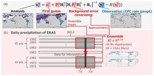
Figure 1 The schematic images of (a) the interpolation method and (b) the construction of an ensemble in this study using ensemble data assimilation. The rain gauge observations from the CPC product are used for the observation ${\mathit{y}}_t^{\mathrm{o}}$. The ensemble ${\mathbf{X}}_t^{\mathrm{b}}$ is obtained from the daily precipitation data of the fifth generation of the ECMWF's reanalysis (ERA5) before and after the interpolation date and the ensemble mean is used as the first guess ${\mathit{x}}_t^{\mathrm{b}}$. R_t is the observation error covariance. H_t( ) denotes an observation operator that maps the first-guess values to the observed values and H_t is the Jacobian matrix of H_t( ). The background error covariance ${\mathbf{P}}_t^{\mathrm{b}}$ is also approximated from the ensemble. Finally, the interpolated daily global precipitation field is computed as the analysis ${\mathit{x}}_t^{\mathrm{a}}$.

The daily precipitation in the same grid points as ERA5 over land is estimated using CPC_gauge as observation inputs according to Eq. (1), which is the equation of the Kalman filter (Kalman, 1960):

$$\begin{array}{}\text{(1)}& {\mathit{x}}_t^{\mathrm{a}}={\mathit{x}}_t^{\mathrm{b}}+{\mathbf{P}}_t^{\mathrm{b}}{\mathbf{H}}_t^{\mathrm{T}}{\left[{\mathbf{H}}_t{\mathbf{P}}_t^{\mathrm{b}}{\mathbf{H}}_t^{\mathrm{T}}+{\mathbf{R}}_t\right]}^{-\mathrm{1}}\left({\mathit{y}}_t^{\mathrm{o}}-H_t\left({\mathit{x}}_t^{\mathrm{b}}\right)\right),\end{array}$$

where ${\mathit{x}}_t^{\mathrm{a}}\in {\mathbb{R}}^N$, ${\mathit{x}}_t^{\mathrm{b}}{\mathbb{R}}^N$ and ${\mathit{y}}_t^{\mathrm{o}}\in {\mathbb{R}}^P$ denote the analysis, first guess and observation values at time t. ${\mathbf{P}}_t^{\mathrm{b}}\in {\mathbb{R}}^{N\times N}$ and ${\mathbf{R}}_t\in {\mathbb{R}}^{P\times P}$ represent the background and observation error covariance matrices. The scalars N and P denote the number of grid points of ERA5 over land and that of the CPC_gauge pixels, respectively. H_t( ) denotes an observation operator that maps the first guess to the observed values and ${\mathbf{H}}_t\in {\mathbb{R}}^{P\times N}$ is the Jacobian matrix of H_t( ). Since we assume that the observation sites are located at the center of the 0.5° pixels, each observation site corresponds exactly to one 0.25° grid point of the first guess. Hence, in our study, the observation operator H_t( ) is simply a linear function which extracts the first-guess data at grid points where the observation exists and H_t is equivalent to H_t( ).

Here, we define R_t as a diagonal matrix owing to the assumption that the errors of the observations are independent of each other. The error variance of each observation (i.e., the diagonal components of R_t) is given by Eq. (2), based on the Lien et al. (2016) suggestion about the effectiveness of logarithm transformation for precipitation variables:

$$\begin{array}{}\text{(2)}& \mathrm{error}\mathrm{variance}=\left\{\begin{array}{ll}\log \left(\mathrm{2}\right)& \left(y_{l,t}^{\mathrm{o}}\le \mathrm{1.0}\mathrm{mm}{\mathrm{d}}^{-\mathrm{1}}\right),\\ \log \left(y_{l,t}^{\mathrm{o}}+\mathrm{1}\right)& \left(y_{l,t}^{\mathrm{o}}>\mathrm{1.0}\mathrm{mm}{\mathrm{d}}^{-\mathrm{1}}\right),\end{array}\right.\end{array}$$

where log is the natural logarithm and $y_{l,t}^{\mathrm{o}}$ denotes the observation at the lth pixel and tth time step from CPC_gauge. As described in Eq. (2), there is a minimum limit (log(2)) to the error variance, which prevents the inverse of R_t from diverging in Eqs. (7), (9) and (10) mentioned below. We also performed sensitivity experiments for a coefficient that multiplies the logarithm-transformed value in Eq. (2), and consequently the value 1.0 was selected as the coefficient (i.e., equivalent to placing no coefficient). An example of the spatial distribution of the error variances is shown in Appendix A.

The first-guess values of ${\mathit{x}}_t^{\mathrm{b}}$ and the background error covariance ${\mathbf{P}}_t^{\mathrm{b}}$ are given by the daily precipitation of ERA5. For each estimation date, the data of the 10 years before and after that date are extracted, considering that CPC_est uses the 20-year average daily precipitation as the first guess for estimation (Xie et al., 2007). Then, we extract the data of the same day of the year as the estimation date and also the surrounding 7 d within those 20 years and we utilize them as an ensemble ${\mathbf{X}}_t^{\mathrm{b}}$ (Fig. 1b) that represents the daily climatology of that date. We do not extract the ERA5 data in the exact year of the estimation date, because we compare our precipitation estimates with ERA5 itself for validation (the details are explained in Sect. 2.2.2). Thereafter, the first guess ${\stackrel{\mathrm{‾}}{x}}_t^{\mathrm{b}}$ is given by the mean of the ensemble. Additionally, ${\mathbf{P}}_t^{\mathrm{b}}$ is approximated by the ensemble (Evensen, 1994) and given by

$$\begin{array}{}\text{(3)}& {\displaystyle }& {\displaystyle }{\mathbf{P}}_t^{\mathrm{b}}\approx {\mathbf{Z}}_t^{\mathrm{b}}{\left({\mathbf{Z}}_t^{\mathrm{b}}\right)}^{\mathrm{T}},\text{(4)}& {\displaystyle }& {\displaystyle }{\mathbf{Z}}_t^{\mathrm{b}}={\displaystyle \frac{\mathit{\delta }{\mathbf{X}}_t^{\mathrm{b}}}{\sqrt{M-\mathrm{1}}}},\end{array}$$

where $\mathit{\delta }{\mathbf{X}}_t^{\mathrm{b}}\in {\mathbb{R}}^{N\times M}$ denotes the ensemble perturbation between the respective ensemble and the ensemble mean for each grid and M denotes the number of ensemble members (M=15 d × 20 years).

Ensemble data assimilation usually requires localization so that the observation values are weighted according to their distance from the analysis grid point using the localization function. When the distance between a grid point in the first guess and an observation site is d km, the localization function L(d) is expressed by the Gaussian function, which is widely used for localization in the LETKF algorithm (e.g., Miyoshi and Yamane, 2007):

$$\begin{array}{}\text{(5)}& L\left(d\right)=\left\{\begin{array}{ll}\exp \left(-\frac{d^{\mathrm{2}}}{\mathrm{2}{\mathit{\sigma }}^{\mathrm{2}}}\right)& d<\mathrm{2}\sqrt{\mathrm{10}/\mathrm{3}}\mathit{\sigma },\\ \mathrm{0}& \mathrm{else},\end{array}\right.\end{array}$$

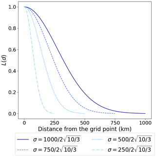
where σ denotes the localization scale (km). Localization is performed by dividing the diagonal component of R_t by L(d) for each grid point and observation site (i.e., the center of a 0.5°×0.5° pixel), so that observations distant from that grid point have less weight. The second row of Eq. (5) truncates the observations where $d\ge \mathrm{2}\sqrt{\mathrm{10}/\mathrm{3}}\mathit{\sigma }$, based on Miyoshi et al. (2007). Here, we determine the value of σ based on the method of Schraff et al. (2016), known as the observation number limit technique. First, a certain distance $d_{\max }^{\mathrm{ini}}$ (km) is set, followed by the maximum number of observation sites ($P_{\mathrm{loc}}^{\max }$) to be used for the estimation. Next, the localization scale σ is determined by Eq. (6):

$$\begin{array}{}\text{(6)}& \mathit{\sigma }=\left\{\begin{array}{ll}\frac{d_{\max }^{\mathrm{ini}}}{\mathrm{2}\sqrt{\mathrm{10}/\mathrm{3}}}& P_{\mathrm{loc}}^{\mathrm{ini}}<P_{\mathrm{loc}}^{\max },\\ \frac{d_{\max }^{\mathrm{fix}}}{\mathrm{2}\sqrt{\mathrm{10}/\mathrm{3}}}& \mathrm{else},\end{array}\right.\end{array}$$

where $P_{\mathrm{loc}}^{\mathrm{ini}}$ denotes the number of observation sites within the $d_{\max }^{\mathrm{ini}}$ km radius from the grid point and $d_{\max }^{\mathrm{fix}}$ is the distance (km) between the grid point and the ($P_{\mathrm{loc}}^{\max }+\mathrm{1}$)th nearest observation site. The tunable parameters $d_{\max }^{\mathrm{ini}}$ and $P_{\mathrm{loc}}^{\max }$ are set to 1000 km and 10, respectively, owing to the authors' preliminary experiments explained in Appendix B. Additionally, examples of L(d) values with different σ values are shown in Appendix C.

Our study applies the LETKF algorithm, in which the ensemble mean of the analysis ${\stackrel{\mathrm{‾}}{\mathit{x}}}_t^{\mathrm{a}}$ is computed by Eq. (7) (Hunt et al., 2007):

$$\begin{array}{}\text{(7)}& {\stackrel{\mathrm{‾}}{\mathit{x}}}_t^{\mathrm{a}}={\stackrel{\mathrm{‾}}{\mathit{x}}}_t^{\mathrm{b}}+{\mathbf{Z}}_t^{\mathrm{b}}{\stackrel{\mathrm{̃}}{\mathbf{P}}}_t^{\mathrm{a}}{\left({\mathbf{H}}_t{\mathbf{Z}}_t^{\mathrm{b}}\right)}^{\mathrm{T}}{\mathbf{R}}_{t\mathrm{loc}}^{-\mathrm{1}}\left({\mathit{y}}_t^{\mathrm{o}}-H_t\left({\mathit{x}}_t^{\mathrm{b}}\right)\right),\end{array}$$

where ${\mathbf{R}}_{t\mathrm{loc}}^{-\mathrm{1}}\in {\mathbb{R}}^{P_{\mathrm{loc}}\times P_{\mathrm{loc}}}$ denotes the inverse of R_t with the localization. The scaler P_loc denotes the number of observations within the localization cutoff radius. Here, we compute ${\stackrel{\mathrm{̃}}{\mathbf{P}}}_t^{\mathrm{a}}$ using the following equations proposed by Kotsuki and Bishop (2022):

$$\begin{array}{}\text{(8)}& {\displaystyle }& {\displaystyle }{\stackrel{\mathrm{̃}}{\mathbf{P}}}_t^{\mathrm{a}}=\mathbf{C}{\left(\mathbf{I}+\mathbf{\Gamma }\right)}^{-\mathrm{1}}{\mathbf{C}}^{\mathrm{T}},\text{(9)}& {\displaystyle }& {\displaystyle }\mathbf{C}={\left({\mathbf{H}}_t{\mathbf{Z}}_t^{\mathrm{b}}\right)}^{\mathrm{T}}{\mathbf{R}}_{t\mathrm{loc}}^{-\mathrm{1}/\mathrm{2}}\mathbf{E}{\mathbf{\Gamma }}^{-\mathrm{1}/\mathrm{2}},\end{array}$$

where I denotes the identity matrix and the eigenvalue decomposition is solved for a P_loc×P_loc matrix given by

$$\begin{array}{}\text{(10)}& {\mathbf{R}}_{t\mathrm{loc}}^{-\mathrm{1}/\mathrm{2}}{\mathbf{H}}_t{\mathbf{Z}}_t^{\mathrm{b}}{\left({\mathbf{H}}_t{\mathbf{Z}}_t^{\mathrm{b}}\right)}^{\mathrm{T}}{\mathbf{R}}_{t\mathrm{loc}}^{-\mathrm{1}/\mathrm{2}}=\mathbf{E}\mathbf{\Gamma }{\mathbf{E}}^{\mathrm{T}}.\end{array}$$

Because the number of local observations P_loc(≤10) is smaller than the ensemble size M(=300), the computational cost is lower than the original LETKF algorithm, in which the eigenvalue decomposition is solved for an M×M matrix $({\stackrel{\mathrm{̃}}{\mathbf{P}}}_t^{\mathrm{a}}{)}^{-\mathrm{1}}$.

Consequently, ${\stackrel{\mathrm{‾}}{\mathit{x}}}_t^{\mathrm{a}}$ is the interpolated daily global precipitation field and is used as the final estimate of this study (hereafter LETKF_est). Based on the method explained above, we estimated the daily global precipitation field for 10 years (1981–1990). Note that we skip the estimation for 23 d during the estimation period, when no valid rain gauge observations were available in either Africa, Eurasia or Canada.

2.2 Validation methods

2.2.1 Data used for the validations

Rain gauge observation data from two precipitation products are used for validations. The first data are from APHRODITE (Yatagai et al., 2012a, b [data set]), which is also a daily precipitation dataset constructed by applying interpolation based on rain gauge observations. In addition to the rain gauge data from the GTS, APHRODITE uses rain gauge data pre-compiled by other projects or organizations and those originally collected from national hydrological and meteorological services. The use of such rain gauge data enables validation against rain gauge observations independent of those used in CPC_est. Here, we use the 0.5°×0.5° pixel data of the latest version of APHRODITE (V1101) covering Monsoon Asia (MA) (Fig. 2a), where particularly dense rain gauge data other than those from the GTS are available in the APHRODITE product.

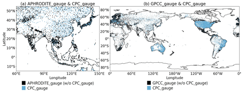
Figure 2 Examples of (a) the distribution of the daily rain gauge observations used in APHRODITE v1101 and the CPC product in Monsoon Asia (on 15 November 1988) and (b) the monthly rain gauge observations used in the GPCC FD product v2022 and the CPC product (in November 1988). The black pixels include more than one rain gauge station, which are independent of the stations used in the CPC product, and the light-blue pixels include more than one rain gauge station used in the CPC product.

Secondly, the monthly precipitation product of the Global Precipitation Climatology Centre (GPCC) is used. The Full Data Reanalysis (FD) product of the GPCC is constructed based on rain gauge observations from >40 000 stations throughout the globe, including not only the observations used in CPC_est, but also data provided by other sources such as the national data of the World Meteorological Organization or the collection of the Global Historical Climatology Network (Becker et al., 2013). Thus, albeit on a monthly basis, the GPCC provides rain gauge observations independently of CPC_gauge on a global scale (Fig. 2b). In this study, we use the latest version of the 0.5°×0.5° pixel FD product (v2022) (Schneider et al., 2022 [data set]).

The objective of this study is to improve the accuracy of rain-gauge-based precipitation fields on a global scale. Considering that the MA APHRODITE product in MA has a limitation in area and that the GPCC product has one in its temporal resolution, we perform validations against both of the data for more comprehensive evaluations.

For both the APHRODITE and GPCC products, we use the data samples of the pixels in which more than one rain gauge is included (APHRODITE_gauge and GPCC_gauge) and assume that the rain gauge(s) is (are) located at the center of each pixel, similar to CPC_gauge. Prior to the validations, the 0.25°×0.25° gridded LETKF_est and ERA5 data are converted into 0.5°×0.5° pixel data so as to be equivalent to the spatial resolutions of CPC_est, APHRODITE_gauge and GPCC_gauge. The details of the conversion method are described in Appendix D.

2.2.2 Validation against APHRODITE_gauge

Here, we use an index that measures correlation based on the rank of the samples rather than their exact magnitude, considering that some studies have suggested the possibility that the APHRODITE precipitation underestimates annual, monthly and daily precipitation in Southeast Asia (Kotsuki and Tanaka, 2013) and South Asia (Ji et al., 2020). Such an index is also less susceptible to low-frequency extreme values, which may occur in daily precipitation data. Hence, Kendall's rank correlation coefficient τ_b (Kendall, 1948) is computed against the daily precipitation of APHRODITE_gauge for LETKF_est, CPC_est and ERA5, respectively, using the data during the whole estimation period of this study (1981–1990). When N_aphro is the number of APHRODITE_gauge pixels and (u_i, v_i) (i=1, …, N_aphro) are the pairs of daily precipitation data to be compared (i.e., the precipitation estimates and APHRODITE_gauge), τ_b is obtained using Eqs. (11) and (12):

$$\begin{array}{}\text{(11)}& {\displaystyle }& {\displaystyle }{\mathit{\tau }}_{\mathrm{b}}={\displaystyle \frac{A-B}{\sqrt{S-T_u}\sqrt{S-T_v}}},\text{(12)}& {\displaystyle }& {\displaystyle }S={\displaystyle \frac{N_{\mathrm{aphro}}\left(N_{\mathrm{aphro}}-\mathrm{1}\right)}{\mathrm{2}}},\end{array}$$

where A (B) represents the total number of cases in which the magnitude relationship of u_j (j=1,
,…, N_aphro) and u_k ($k=j+\mathrm{1}$, …, N_aphro) is concordant (discordant) with that of v_j and v_k. T_u and T_v denote the number of ties in u_i and v_i, respectively.

The value of τ_b closer to 1.0 (−1.0) indicates stronger positive (negative) correlation between the two types of data. Because the computation of τ_b neglects the samples with the exact same values in APHRODITE_gauge (or in the precipitation estimates) and because there is more than one no-rain case in APHRODITE_gauge or the precipitation estimates, it should be mentioned that τ_b cannot measure the similarity of no-rain cases between the two data. We exclude the samples of the pixels where the input observations from CPC_gauge are available to evaluate only the interpolated precipitation in our study. Furthermore, we exclude the samples of the pixels where the precipitation of APHRODITE_gauge is <0.5 mm d⁻¹, considering that precipitation below this value generally cannot be measured precisely by rain gauges.

2.2.3 Validations against GPCC_gauge

The spatial root mean square difference (RMSD), mean absolute difference (MAD) and Pearson's correlation coefficient (R) are computed for each month during the whole estimation period (1981–1990) against the monthly precipitation of GPCC_gauge for LETKF_est and CPC_est following Eqs. (13)–(15):

$$\begin{array}{}\text{(13)}& {\displaystyle }\mathrm{spatial}{\mathrm{RMSD}}_t=\sqrt{{\displaystyle \frac{\sum _{i=\mathrm{1}}^{N_{\mathrm{gpcc}}}{w}_i{\left(x_{\mathrm{gpcc}i,t}-x_{\mathrm{est}i,t}\right)}^{\mathrm{2}}}{\sum _{i=\mathrm{1}}^{N_{\mathrm{gpcc}}}{w}_i}}},\text{(14)}& {\displaystyle }\mathrm{spatial}{\mathrm{MAD}}_t={\displaystyle \frac{\sum _{i=\mathrm{1}}^{N_{\mathrm{gpcc}}}{w}_i\left|x_{\mathrm{gpcc}i,t}-x_{\mathrm{est}i,t}\right|}{\sum _{i=\mathrm{1}}^{N_{\mathrm{gpcc}}}{w}_i}},\text{(15)}& {\displaystyle }\begin{array}{rl}& R_t=\\ & {\displaystyle \frac{\frac{\mathrm{1}}{N_{\mathrm{gpcc}}}\sum _{i=\mathrm{1}}^{N_{\mathrm{gpcc}}}\left(x_{\mathrm{gpcc}i,t}-\stackrel{\mathrm{‾}}{x_{\mathrm{gpcc}t}}\right)\left(x_{\mathrm{est}i,t}-\stackrel{\mathrm{‾}}{x_{\mathrm{est}t}}\right)}{\sqrt{\frac{\mathrm{1}}{N_{\mathrm{gpcc}}}\sum _{i=\mathrm{1}}^{N_{\mathrm{gpcc}}}{\left(x_{\mathrm{gpcc}i,t}-\stackrel{\mathrm{‾}}{x_{\mathrm{gpcc}t}}\right)}^{\mathrm{2}}}\sqrt{\frac{\mathrm{1}}{N_{\mathrm{gpcc}}}\sum _{i=\mathrm{1}}^{N_{\mathrm{gpcc}}}{\left(x_{\mathrm{est}i,t}-\stackrel{\mathrm{‾}}{x_{\mathrm{est}t}}\right)}^{\mathrm{2}}}}},\end{array}\end{array}$$

where N_gpcc denotes the number of GPCC_gauge pixels. x_gpcc i,t and x_est i,t denote the monthly precipitation of GPCC_gauge and the estimates (LETKF_est or CPC_est) at the ith pixel and tth time step, respectively. Additionally, $\stackrel{\mathrm{‾}}{x_{\mathrm{gpcc}t}}$ and $\stackrel{\mathrm{‾}}{x_{\mathrm{est}t}}$ denote the spatial mean monthly precipitation of GPCC_gauge and the estimates (LETKF_est or CPC_est) at the tth time step, respectively. Here, w_i=cos (θ_i) is the latitude-dependent weight of the ith pixel, where θ is the latitude.

Smaller RMSD or MAD values (at the minimum of 0.0) indicate that the two data are similar, while the R value closer to 1.0 (−1.0) indicates a stronger positive (negative) correlation. As explained in Sect. 2.2.2, we also exclude the samples of the pixels where the input observations from CPC_gauge are available for the validations against GPCC_gauge. Additionally, the months in which we skipped the estimation for daily precipitation (as noted in Sect. 2.1.2) were excluded from the validations (January 1981; April 1983; January 1984; January–February and July–August 1985; January, March, September and November 1986).

3 Results

First-guess precipitation fields used in our study, CPC_gauge and LETKF_est on 15 November 1988, are illustrated as examples in Fig. 3a, b and d, respectively. The daily precipitation field of LETKF_est (Fig. 3d) is interpolated using the smooth and averaged climatological first guess (Fig. 3a) and the sparsely located rain gauge observations (Fig. 3b), using the methodology presented in Sect. 2.1.2. For the same date, the daily precipitation of NOAA's CPC_est, which is also estimated by OI using the rain gauge observations in CPC_gauge, is depicted in Fig. 3c for comparison. Although the precipitation patterns of CPC_est (Fig. 3c) and LETKF_est (Fig. 3d) are overall similar to each other, several differences exist between them. For example, broader precipitating areas are seen for LETKF_est than for CPC_est, especially around central Africa, South America and the Indochinese Peninsula. Precipitation areas can be seen around the Himalayas and the Zagros Mountains in LETKF_est but not in CPC_est. In addition, the precipitation is generally weaker for LETKF_est than for CPC_est.

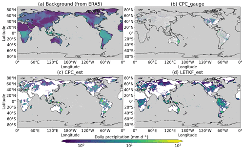
Figure 3 Examples of the precipitation fields (mm d⁻¹) for (a) the first guess used in our study, (b) the rain gauge observations of CPC_gauge and the global precipitation estimates of (c) CPC_est and (d) LETKF_est (on 15 November 1988). Pixels on the ocean are colored in gray for all the subplots as well as those where no rain gauge observations are available for subplot (b). Pixels are colored in white when the precipitation is <0.5 mm d⁻¹.

The scatterplots in Fig. 4 compare the daily precipitation of ERA5, CPC_est and LETKF_est with APHRODITE_gauge at pixels in MA, showing that LETKF_est is aligned with APHRODITE_gauge the most compared to ERA5 and CPC_est. Furthermore, the τ_b value (described in Sect. 2.2.2) of LETKF_est computed against APHRODITE_gauge is the highest (Fig. 4), with statistically significant differences at the P value of 0.01, notwithstanding the fact that LETKF_est was converted to 0.5°×0.5° pixel data in advance of this validation. Therefore, this shows that the daily precipitation of LETKF_est is more similar to that of APHRODITE_gauge than ERA5 or CPC_est in terms of Kendall's rank correlation coefficient.

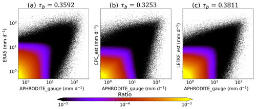
Figure 4 Scatterplots comparing the daily precipitation (mm d⁻¹) of APHRODITE_gauge with that of (a) ERA5, (b) CPC_est and (c) LETKF_est. The colors represent the ratio of samples within each 0.1 mm d⁻¹ × 0.1 mm d⁻¹ bin in each two-dimensional histogram. Kendall's rank correlation coefficients (τ_b) of (a) ERA5, (b) CPC_est and (c) LETKF_est computed against APHRODITE_gauge are listed at the top of each subplot.

The spatial RMSD, MAD and R verified against GPCC_gauge (described in Sect. 2.2.3) indicate that the monthly precipitation of LETKF_est shows better agreement with GPCC_gauge (i.e., lower RMSD and MAD values and higher R values) than that of CPC_est for all the months throughout the estimation period (Fig. 5). The temporal averages of the spatial RMSD and MAD of LETKF_est are lower than those of CPC_est by 14.79 % and 10.96 %, respectively. The spatial MAD is also computed separately in the low-latitude region (20° N–20° S) and the mid- and high-latitude regions (90–20° N and 20–90° S) against GPCC_gauge for both LETKF_est and CPC_est for each month. Figure 6 indicates that the MAD values in the low-latitude region are generally higher than those in the mid- and high-latitude regions. However, the scatterplots for the low-latitude region are more divergent from the 1:1 line upwards, indicating that the MAD values have improved for LETKF_est compared to CPC_est, particularly in this region. Therefore, this indicates that our estimation method is more beneficial than OI, especially for the low-latitude region, which is highly occupied by the tropical regions with more precipitation.

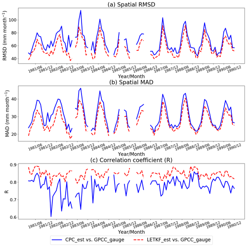
Figure 5 The time series of (a) the spatial root mean square difference (RMSD; millimeters per month), (b) the spatial mean absolute difference (MAD; millimeters per month) and (c) Pearson's correlation coefficient (R), verified against GPCC_gauge. The blue solid and red dashed lines represent CPC_est and LETKF_est, respectively. The validations are not performed for the months in which we skipped the estimation of daily precipitation (January 1981; April 1983; January 1984; January–February and July–August 1985; January, March, September and November 1986).

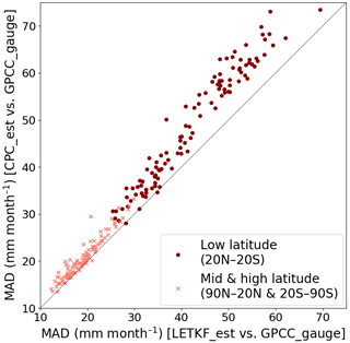
Figure 6 Scatterplots comparing the spatial MAD (millimeters per month) of CPC_est and LETKF_est verified against the monthly precipitation of GPCC_gauge. Dark-red circles and light-red cross marks represent the low-latitude region (20° N–20° S) and mid- and high-latitude regions (90–20° N and 20–90° S), respectively.

4 Discussion

The main reason for the improvement in the accuracy of LETKF_est compared to CPC_est is presumably the interpolation method that uses the dynamically consistent first guess and background error covariance constructed from the ERA5 data. This would have led to the improvement in the accuracy of the first guess as well as the variance of each grid point and the covariance between paired grid points. For example, our first guess would take into account the orographic effects. Here, we first investigate the difference in South Asian precipitation, showing an example on an arbitrarily selected date in the monsoon season.

Figure 7 depicts the first guess used for this study and the daily precipitation of CPC_gauge, ERA5, CPC_est and LETKF_est on 27 June 1985. It should be noted that the precipitation of LETKF_est (Fig. 7f) is the one converted into 0.5°×0.5° pixel data for the comparison with that of CPC_est (Fig. 7e). LETKF_est succeeds in reproducing the orographic changes in precipitation around the Himalayas (Fig. 7f) despite the lack of observation inputs in the surrounding area (Fig. 7c), while CPC_est fails to do so (Fig. 7e). Although the first guess of CPC_est is also adjusted considering orographic effects prior to interpolation by OI (Xie et al., 2007), Fig. 7e indicates that this adjustment would be insufficient. The first guess constructed by ERA5 (Fig. 7b) is presumed to contribute to these precipitation patterns of LETKF_est, since it clearly reflects orographic features similar to the original ERA5 (Fig. 7d). On the other hand, as explained in Sect. 3, the precipitation of LETKF_est has better agreement with APHRODITE_gauge than that of ERA5 itself, suggesting that not only the first guess but also the climatological background error covariance constructed from ERA5 contribute to the improvement in our estimates. It should be noted that orographic effects at a finer scale may be suboptimal in our estimation method, in which the rain gauge sites are assumed to be located at the center of 0.5°×0.5° pixels. Furthermore, the performance of our proposed method may also differ if different reanalysis data are used, because reanalysis data with better quality would provide a better first guess and error covariance.

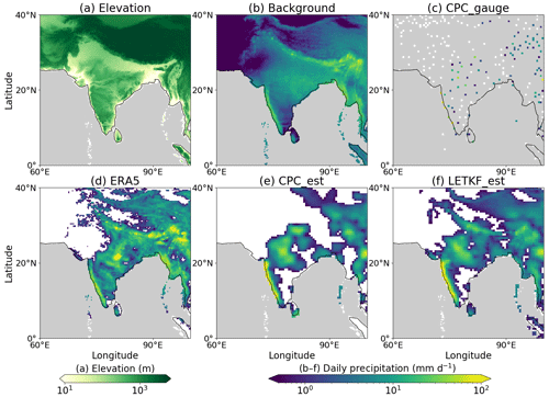
Figure 7 (a) The elevation (m) and examples of (b) the first guess constructed in our study (mm d⁻¹), (c) the rain gauge observations of CPC_gauge (mm d⁻¹) and the global precipitation estimates (mm d⁻¹) of (d) ERA5, (e) CPC_est and (f) LETKF_est (on 27 June 1985) around India. Pixels on the ocean are colored in gray for all the subplots, together with those where no rain gauge observations are available for subplot (c). The precipitation of LETKF_est (f) is the one converted into 0.5°×0.5° pixel data. Pixels are colored in white when the precipitation is <0.5 mm d⁻¹.

To investigate whether the precipitation of LETKF_est is more accurate than that of CPC_est around mountainous areas such as the Himalayas, not only on a specific date but also for the whole estimation period, Kendall's rank correlation coefficient (τ_b) was computed for LETKF_est and CPC_est against the daily precipitation of APHRODITE_gauge for each pixel where more than 1800 samples of APHRODITE_gauge were available during the whole estimation period (1981–1990) in MA. The results in Fig. 8 show that the τ_b values of LETKF_est are higher than those of CPC_est by >0.05, especially around the Himalayas, indicating that the method of this study improves the daily precipitation largely around this area during the estimation period.

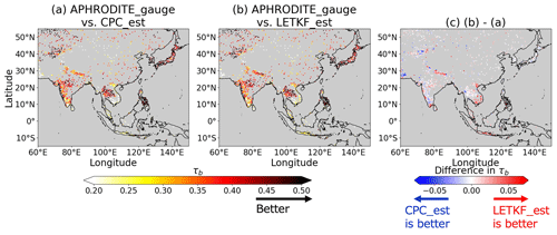
Figure 8 Kendall's rank correlation coefficient (τ_b) computed against the daily precipitation of APHRODITE_gauge for (a) CPC_est and (b) LETKF_est at each pixel. Subplot (c) represents the difference between subplots (b) and (a). Darker colors in subplots (a) and (b) indicate that the precipitation estimates are more similar to APHRODITE_gauge. Warm colors in subplot (c) indicate that LETKF_est is more similar to APHRODITE_gauge than CPC_est and cold colors indicate otherwise. τ_b is only computed at pixels where more than 1800 samples from APHRODITE_gauge are available and the pixels are colored in gray if they do not match this condition.

Additionally, the temporal MAD values of LETKF_est and CPC_est are computed for the global area against the monthly precipitation of GPCC_gauge at each pixel where more than 50 samples of GPCC_gauge are available, using Eq. (16):

$$\begin{array}{}\text{(16)}& \mathrm{temporal}{\mathrm{MAD}}_i={\displaystyle \frac{\sum _{t=\mathrm{1}}^T\left|x_{\mathrm{ref}i,t}-x_{\mathrm{est}i,t}\right|}{T}},\end{array}$$

where T is the total number of monthly time steps during the whole estimation period (1981–1990). The spatial MAD (described in Sect. 2.2.3) shows the similarity between two data on the global scale for each month, whereas the temporal MAD shows the similarity between two data for the whole period at each pixel.

Figure 9 depicts the temporal MAD computed in the Asian and African regions. The results for the global area are also shown in Appendix E. The temporal MAD of LETKF_est is smaller than that of CPC_est by >10 mm per month at many pixels around mountainous areas, such as the Himalayas (Fig. 9c) and the Zagros Mountains (Fig. 9f), indicating that the estimation method of this study is beneficial for these areas throughout the estimation period. Furthermore, the temporal MAD of LETKF_est decreased by >10 mm per month compared to that of CPC_est in regions where rain gauge stations are especially sparse, such as some regions in Southeast Asia (Fig. 9c) or between 0 and 20° S in Africa (Fig. 9f). In both the mountainous and rain-gauge-sparse regions, the temporal MAD is relatively high compared to other regions (Fig. 9a, b and d, e). Therefore, although interpolating precipitation fields in such areas is especially difficult, it is presumed that the proposed method succeeded in improving the accuracy of the estimates compared to the conventionally used OI method. Moreover, the 10-year experiment of our study was completed in <12 h (i.e., <12 s to estimate a daily global precipitation field) using 20 cores in the computer processing unit AMD EPYC Rome 7402, indicating the expected computational efficiency of the LETKF algorithm as mentioned in Sect. 1. Since reanalysis data cover variables other than precipitation, there is also a possibility that our proposed method will be applicable to variables such as soil moisture, depending on the accuracy, frequency and spatial density of its observations.

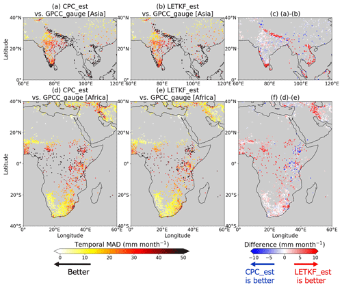
Figure 9 The temporal MAD (millimeters per month) of CPC_est (a, d) and LETKF_est (b, e) computed against the monthly precipitation of GPCC_gauge at each pixel. Subplots (c) and (f) represent the differences (millimeters per month) between subplots (a, d) and (b, e), respectively. Lighter colors in subplots (a), (b), (d) and (e) indicate that the precipitation estimates are more similar to GPCC_gauge. Warm colors in subplots (c) and (f) indicate that LETKF_est is more similar to GPCC_gauge than CPC_est and cold colors indicate otherwise. The temporal MAD is only computed at pixels where more than 50 samples from GPCC_gauge are available and the pixels are colored in gray if they do not match this condition.

There are some remaining limitations of this study that should be dealt with in the future. Firstly, our study has applied no transformation for the probability distributions of daily precipitation prior to the estimation, even though the precipitation variable can be less Gaussian. Many previous studies have pointed out that the analysis may not match the solution of the Bayesian estimation when data assimilation based on minimum variance estimation is applied to variables that are known to diverge from Gaussian ones, making it difficult to obtain an optimal analysis (e.g., Posselt and Bishop, 2012; Kotsuki et al., 2017). This problem may occur significantly for regions where the precipitation amount is small, considering the fact that the ensemble used in the estimation may contain many samples near 0.0 mm d⁻¹ for such regions. As such, although the proposed method outperformed OI in general, there is a possibility that the accuracy of the precipitation estimates will be improved further by applying treatments to non-Gaussianity such as Gaussian transformation (Lien et al., 2013; Kotsuki et al., 2017) or gamma–inverse-gamma–Gaussian ensemble Kalman filtering (Bishop, 2016).

Another limitation is the lack of validation sites in specific regions. For example, the density of the rain gauges used in CPC_gauge is especially high in North America, making it difficult to perform validations against rain gauge observations independently of the observation inputs of the estimation (Fig. 2b) in this region. On the other hand, both the rain gauges in CPC_gauge and other independent rain gauges used in GPCC_gauge are sparse in central Australia and the Arabian Peninsula (Fig. 2b). Therefore, validations may be biased by the results of the regions with a large number of rain gauges that are independent of CPC_gauge.

5 Conclusions

This study proposed a new estimation method for daily global precipitation fields from rain gauge observations using the algorithm of the LETKF in which the first guess and its error covariance are developed based on the precipitation from the reanalyzed precipitation of ERA5. We succeeded in estimating the daily global precipitation fields with high computational efficiency (i.e., <12 s d⁻¹). Our findings can be summarized as follows.

Our estimates showed better agreement with rain gauge observations compared to the existing product of the NOAA CPC. Because we utilized the same rain gauge observations for the inputs of our estimation as those used for the NOAA CPC product, our results indicate that the proposed estimation method outperformed that of the NOAA CPC (i.e., OI). Our proposed method had the advantage of constructing a dynamically consistent first guess and background error variance using reanalysis data for interpolating precipitation fields. Additionally, the method of this study was shown to be particularly beneficial for mountainous or rain-gauge-sparse regions.

There are some remaining limitations of this study, e.g., treatments on the less Gaussian distribution of the precipitation variable and the discrepancies between the regions regarding the density of the validation sites. Despite such limitations, the present study succeeded in improving the accuracy of precipitation fields estimated from rain gauge observations, which will lead to more effective use of spatially sparse rain gauge observations.

Appendix A: Spatial distribution of observation error variances in our study

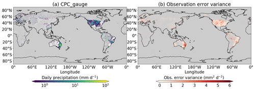
Figure A1 Examples of (a) the rain gauge observations of CPC_gauge (mm d⁻¹) and (b) the observation error variance (mm² d⁻²) (on 15 November 1988). Pixels where no rain gauge observations are available are colored in gray for both subplots. Pixels are colored in white when the precipitation is <0.5 mm d⁻¹ in subplot (a).

Appendix B: Sensitivity analysis of the localization parameters

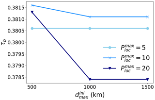
First, 10-year experiments from 1981 to 1990 were performed to estimate daily global precipitation fields using the methodology described in Sect. 2.1.2 with different combinations of the localization parameters $d_{\max }^{\mathrm{ini}}(=\mathrm{500},\mathrm{1000},\mathrm{1500}\mathrm{km})$ and $P_{\mathrm{loc}}^{\max }(=\mathrm{5},\mathrm{10},\mathrm{20})$. Next, the validation against APHRODITE_gauge described in Sect. 2.2.2 is performed for the precipitation estimates of each experiment. The results of the validations show that Kendall's rank correlation coefficient τ_b is highest when $d_{\max }^{\mathrm{ini}}=\mathrm{500}$ km and $P_{\mathrm{loc}}^{\max }=\mathrm{10}$, followed by when $d_{\max }^{\mathrm{ini}}=\mathrm{500}$ km and $P_{\mathrm{loc}}^{\max }=\mathrm{20}$ and when $d_{\max }^{\mathrm{ini}}=\mathrm{1000}$ km and $P_{\mathrm{loc}}^{\max }=\mathrm{10}$ (Fig. B1). Because some grid points in Africa were found to have no observation point within a 500 km radius, values $d_{\max }^{\mathrm{ini}}=\mathrm{1000}$ km and $P_{\mathrm{loc}}^{\max }=\mathrm{10}$ were eventually selected for the localization parameters in the experiment described in the main text.

Figure B1 Kendall's rank correlation coefficient computed against APHRODITE_gauge for different combinations of the localization parameters $d_{\max }^{\mathrm{ini}}(=\mathrm{500},\mathrm{1000},\mathrm{1500}\mathrm{km})$ and $P_{\mathrm{loc}}^{\max }(=\mathrm{5},\mathrm{10},\mathrm{20})$.

Appendix C: Change in the localization function depending on the distance of a grid point and an observation site

Figure C1 Localization function L(d) depending on the distance of a grid point and an observation site when the localization scale is $\mathit{\sigma }=\frac{\mathrm{1000}}{\mathrm{2}\sqrt{\mathrm{10}/\mathrm{3}}}$, $\frac{\mathrm{750}}{\mathrm{2}\sqrt{\mathrm{10}/\mathrm{3}}}$, $\frac{\mathrm{500}}{\mathrm{2}\sqrt{\mathrm{10}/\mathrm{3}}}$, $\frac{\mathrm{250}}{\mathrm{2}\sqrt{\mathrm{10}/\mathrm{3}}}$ (km).

Appendix D: Method for converting 0.25°×0.25° gridded ERA5 and LETKF_est data into 0.5°×0.5° pixel data

In our study, we assume that the daily precipitation of a 0.25°×0.25° grid point represents that of a 0.25°×0.25° pixel whose center is located at the original grid point. Thus, to convert the 0.25°×0.25° gridded data into 0.5°×0.5° pixel data, we compute the weighted average of the daily precipitation of the 0.25°×0.25° grid points inside each 0.5°×0.5° pixel, depending on the area ratio of the 0.25°×0.25° pixels (Fig. D1). This method allows us to conserve the total precipitation in the global area before and after the conversion.

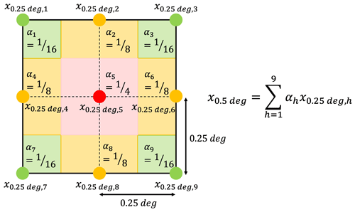
Figure D1 Schematic image of the method for converting 0.25°×0.25° gridded data (the precipitation data of the colored plots) into 0.5°×0.5° pixel data (the precipitation datum of the pixel surrounded by black lines). $x_{\mathrm{0.25}\mathrm{deg},h}(h=\mathrm{1},\mathrm{\dots },\mathrm{9})$ and ${\mathit{\alpha }}_h(h=\mathrm{1},\mathrm{\dots },\mathrm{9})$ denote the daily precipitation and the weight of each 0.25°×0.25° grid point. The daily precipitation of the 0.5°×0.5° pixel x_0.5 deg is computed by the weighted average of $x_{\mathrm{0.25}\mathrm{deg},h}(h=\mathrm{1},\mathrm{\dots },\mathrm{9})$.

Appendix E: Spatial distribution of the temporal MAD for the global area

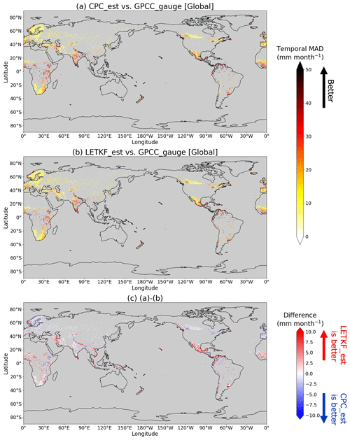
Figure E1 The temporal MAD (millimeters per month) of (a) CPC_est and (b) LETKF_est computed against the monthly precipitation of GPCC_gauge at each pixel in the global area. Subplot (c) represents the differences (millimeters per month) between subplots (a) and (b). Lighter colors in subplots (a) and (b) indicate that the precipitation estimates are more similar to GPCC_gauge. Warm colors in subplot (c) indicate that LETKF_est is more similar to GPCC_gauge than CPC_est and cold colors indicate otherwise. The temporal MAD is only computed at pixels where more than 50 samples from GPCC_gauge are available and the pixels are colored in gray if they do not match this condition.