Drivers of global irrigation expansion: the role of discrete global grid choice

Global statistical irrigation modeling relies on geospatial data and traditionally adopts a discrete global grid based on longitude–latitude reference. However, this system introduces area distortion, which may lead to biased results. We propose using the ISEA3H geodesic grid based on hexagonal cells, enabling efficient and distortion-free representation of spherical data. To understand the impact of discrete global grid choice, we employ a non-parametric statistical framework, utilizing random forest methods, to identify the main drivers of historical global irrigation expansion using, among other data, outputs from the global dynamic vegetation model Lund-Potsdam-Jena managed Land (LPJml).

Irrigation is critical for food security amidst growing populations, changing consumption patterns, and climate change. It significantly boosts crop yields but also alters the water cycle and global water resources. Understanding past irrigation expansion and its drivers is vital for global change research, resource assessment, and the prediction of future trends.

We compare predictive accuracy, simulated irrigation patterns, and identification of irrigation drivers between the two grid systems. Using the ISEA3H geodesic grid system increases the predictive accuracy by up to 28 % compared to the longitude–latitude grid. The model identifies population density, potential productivity increase, evaporation, precipitation, and water discharge as key drivers of historical global irrigation expansion. Gross domestic product (GDP) per capita also shows some influence.

We conclude that the geodesic discrete global grid system significantly affects predicted irrigation patterns and identification of drivers and thus has the potential to enhance statistical modeling, which warrants further exploration in future research across related fields. This analysis lays the foundation for comprehending historical global irrigation expansion.

1 Introduction

About 80 % of data being produced are of geospatial nature (Hahmann and Burghardt, 2013). While the construction of maps and the referencing of locations on the Earth's surface have a very long history, it is becoming increasingly important to find efficient ways to process, integrate, and analyze geospatial data to solve problems in times of globalization. To that end, geographic grid systems are used to project the geographic space into a mathematical space where algorithms and statistical methods can be applied.

The most widely used grid system is the geographic coordinate system (using latitude and longitude lines), which dates back to the third century BCE (McPhail, 2011; Ware et al., 2020). A great advantage of this system is that it can be stored compactly and used easily for computations (Ware et al., 2020). Unfortunately, when portrayed on a sphere, grids based on geographic coordinates suffer from cell area distortion due to the converging lines of equal longitude. In the context of global statistical modeling, this ultimately results in oversampling of the northernmost regions.

A great number of alternative discrete global grid systems (DGGSs) have emerged to fulfill the needs of different research fields and modeling strategies (Kimerling et al., 1994). Since these grid systems offer significant benefits for big data and digital Earth research, there have been numerous advancements, new implementations, and example applications in various fields (Sahr, 2011; Jendryke and McClure, 2019; Sirdeshmukh et al., 2019; Bousquin, 2021, e.g.). Today, standard Earth grid systems, including DGGSs, are documented by the Open Geospatial Consortium (OGC) and the International Organization for Standardization (ISO) (ISO, 2021; Purss, 2015). Even though current implementations might not yet fully comply with all these standards (Bondaruk et al., 2020), there is a clear benefit to starting the integration of these data structures.

In this paper, we propose to use a global DGGS based on a hexagonal tessellation of the Earth's surface in the context of modeling global historical irrigation expansion. This grid was introduced by Sahr et al. (2003) and has gained large popularity in many research contexts. Two recent examples of open-source DGGS libraries that are based on hexagonal grid structures are the H3 system, developed by Uber (2022), and DGGRID (Barnes and Sahr, 2017). Mechenich and Zliobaite (2023) recently presented the Eco-ISEA3H database that consists of global spatial data characterizing climate, geology, land cover, physical and human geography, and the geographic ranges of nearly 900 large mammalian species. In contrast to grid cells induced by the longitude–latitude graticule, hexagonal cells are able to cover almost the entire surface of the Earth without suffering from area distortion. That way, all regions have the same influence in a statistical model.

Recently, hexagonal mesh grids have gained popularity among hydrologists (Li et al., 2022). A group of hydrological functions on hexagonal meshes, such as flow direction and accumulation, stream networks, or watershed boundary extraction, were explored by Liao et al. (2020). The authors show that their algorithm's performance is better when considering the hexagonal-mesh-based output compared to the traditional square-mesh-based output. Wang et al. (2020) studied valley networks and model valley lines based on hexagonal grids. Compared to traditional square grids, the study shows that using the hexagonal grid leads to a higher location accuracy. In another study, Wright (2019) developed a regular hierarchical surface model, where hydrological computation was generalized on hexagonal and triangular grids. Additionally, there has been an increasing interest in managing geospatial data and developing models to solve real-world problems using the open-source DGGRID library (Hojati and Robertson, 2020; Li et al., 2021; Chaudhuri et al., 2021; Robertson et al., 2020; Li et al., 2022).

Our study aims to predict global historical irrigation patterns. Since both rainfed and irrigated grid cells are equally important for our analysis, addressing the issue of area distortion is crucial. To the best of our knowledge, we are the first to utilize the Icosahedral Equal Area Aperture 3 Hexagon Discrete Global Grid System (ISEA3H DGGS) in this context. This grid system enables us to directly analyze global irrigation patterns without area distortion. Additionally, the grid system has potential for improving the mapping of spatial clusters and neighborhood patterns, as each grid cell has a unique set of neighbors.

The second aim of this paper is to contribute to the literature on global irrigation expansion. Irrigation is crucial to ensure the world's food security. A growing human population, shifting consumption patterns, and climate change increase the pressure on agricultural production (Foley et al., 2011). To meet the growing human food demand, irrigation has rapidly increased over the last century as it increases crop yields (Siebert et al., 2015). In the year 2000, approximately 40 % of the global food production was harvested on irrigated land, utilizing only 20 % of the total farming area (Schultz et al., 2005). To achieve this agricultural intensification, a large amount of fresh water is needed. Consequently, irrigation alters the hydrological cycle significantly (Zohaib and Choi, 2020). At a global scale, irrigation is responsible for about 60 % of total fresh water withdrawals and 80 % of total fresh water consumption (Döll et al., 2014; Siebert et al., 2015). It is therefore important to understand the past evolution of irrigation expansion and its main drivers for global change research, the assessment of resources, and the prediction of future developments.

There have been a few studies on the drivers of global irrigation in previous years. Neumann et al. (2011) investigated the global irrigation pattern in the year 2000. Using a multilevel approach, they modeled irrigation as a function of biophysical and socioeconomic factors. Their results show that biophysical factors have a significant influence on irrigation. Additionally, the authors provide suggestive evidence that socioeconomic factors play a role in irrigation. However, it is emphasized that the model suffers from uncertainty due to the lack of spatially explicit socioeconomic information and the possibility of external influences, such as public investments. While our model also faces these limitations, we are able to extend the analysis by including a historical dimension.

Puy et al. (2020) investigated uncertainties in published projections of global irrigation expansion for the year 2050. By comparing different projected estimates of irrigated area to a simple model predicting irrigated area as a function of only population size, constrained by water and land availability, taking into account parametric and model uncertainties, the authors postulate that current models underestimate future irrigated areas. Other recent studies developed global irrigation maps, mostly using a combination of remote sensing, machine learning, and climate data (Meier et al., 2018; Salmon et al., 2015; Nagaraj et al., 2021).

We contribute to the literature on global irrigation expansion by investigating the drivers of the historical expansion between 1902 and 2000, using a novel non-parametric statistical model. We distinguish between the factors that influence the probability of a grid cell being irrigated, i.e., the decision to irrigate instead of remaining rainfed, and the irrigation intensity, once a grid cell is irrigated. We employ a stacked random forest framework to assess the quality between statistical irrigation models based on two different grid systems. Our main focus is on the influence of the grid the data are presented in.

2 Data

Our first objective in this study is to analyze the choice of discrete global grid system for modeling the historical evolution of global irrigation expansion. To achieve this, we focus on the entire global land surface, excluding Antarctica. We consider data from 1902 to 2005 to comprehensively capture the historical evolution of irrigation expansion over the past century.

Our analysis builds on a data set that consists of a simulation output from the Lund-Potsdam-Jena managed Land (LPJml) model (Sitch et al., 2003; Bondeau et al., 2007) and historical economic data from the Maddison Project Database (Inklaar et al., 2018).

LPJml is a process-based dynamical global vegetation, hydrology, and crop model simulating natural and managed vegetation growth based on soil, climate, and management input at a daily resolution and at a global 0.5°×0.5° spatial grid scale, resulting in a total number of 67 420 terrestrial grid cells per time unit in each variable (Schaphoff et al., 2018).

We prescribe an agricultural land use data set based on the History Database of the Global Environment (HYDE) (Klein Goldewijk et al., 2017) with additional assumptions on irrigation systems and extent of areas equipped for irrigation by Jägermeyr et al. (2015) based on the global Historical Irrigation Dataset (HID). One advantage of the HID is that the evolution of land irrigation was implemented using official land use data and is therefore independent of socioeconomic information, such as gross domestic product or population density (Siebert et al., 2015). Hence, the relationship of irrigation and socioeconomic variables can safely be analyzed. As climate input, the Climatic Research Unit Time Series (Harris et al., 2014) is used. Whether a crop actually needs irrigation is internally decided by the LPJml simulation based on biophysical constraints and constrained by surface water availability (Schaphoff et al., 2018).

From the simulation, we obtain the direct output variables precipitation, evaporation, discharge, crop yield, and the actually irrigated fraction for each grid cell. Additionally the median potential increase in crop yield productivity is derived. This is estimated from two separate synthetic simulations, where potential yields for each crop and grid cell are compared with and without irrigation. The variables are aggregated annually for each grid cell to obtain a time series for the years 1901 to 2005.

The LPJml data are complemented by the Maddison Project database on the historical performance of the world economy (Inklaar et al., 2018; Bolt and Zanden, 2014). Of particular interest is the time series of the gross domestic product (GDP) per capita, consisting of estimates of comparative levels of real GDP per capita in recent time periods, combined with long-term time series growth of GDP per capita. Even though the Maddison Project database yields state-of-the-art historical economic data, there are many countries without an estimation of GDP per capita in the time period 1900 to 1960, leading to missing data.

2.1 Variables

We use the fraction of a grid cell that is actually irrigated as the dependent variable. This fraction is a continuous variable between 0 and 1, with 1 meaning a grid cell is fully irrigated, and 0 meaning that none of the area is irrigated. It is important to note that since grid cells in the standard longitude–latitude grid change in area relative to latitude, irrigation fraction values between grid cells are not directly comparable. Figure A2 displays the global irrigation fraction map, based on HID data from 2000.

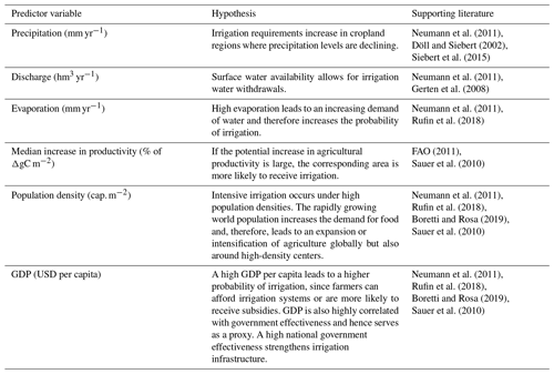
The selection of potential drivers of irrigation expansion was led by the existing literature and data availability (see Table 1). We consider the following variables for explaining irrigation fraction: population density, precipitation, discharge, evaporation, potential yield increase through irrigation, and GDP per capita.

Neumann et al. (2011)Döll and Siebert (2002)Siebert et al. (2015)Neumann et al. (2011)Gerten et al. (2008)Neumann et al. (2011)Rufin et al. (2018)FAO (2011)Sauer et al. (2010)Neumann et al. (2011)Rufin et al. (2018)Boretti and Rosa (2019)Sauer et al. (2010)Neumann et al. (2011)Rufin et al. (2018)Boretti and Rosa (2019)Sauer et al. (2010)

Table 1 Potential predictors and hypotheses.

The GDP-per-capita data are available at a national level and broken down to a 0.5°× 0.5° grid scale, by assigning the country's value to all grid cells in a country. Since there are observations missing, especially in the earlier time periods (see Fig. S2), the variable is split up into the categories “high income”, “upper middle income”, “lower middle income”, “low income”, and “missing”, following the methodology of Hastie et al. (2009) and the World Bank's classification of GDP per capita from 2011 (World Bank, 2011). The classification can be found in the Supplement (Table S1). That way, we treat the missing values as an additional category and are able to include all observations in our analysis.

We report the pairwise Pearson correlation coefficients (Appendix, Table A2) and variance inflation factors (Appendix, Table A3) to investigate multicollinearity between the continuous predictor variables, following the methodology in Rufin et al. (2018). We find that all pairwise Pearson correlation coefficients are below the threshold of 0.7 (Dormann et al., 2013), except for the pair precipitation–evaporation, for which we find a value of 0.72. The variance inflation factors are below the tight threshold of 5, indicating that the predictor variables are sufficiently independent for our analysis (James et al., 2013).

2.2 Descriptive statistics

Overall, the irrigated area expanded throughout the study period. The proportion of grid cells with observed irrigation increased from approximately 10 % in 1902 to about 31 % in 2005. The most significant increases in irrigated area occurred in southeastern Asia, Central and South America, Central America, and eastern Asia. These statistics align with the findings of Siebert et al. (2015), who investigated areas equipped for irrigation.

Despite the expansion of irrigated land, the data are highly imbalanced: throughout the study period, about 75 % of the observed irrigation fractions are zero, whereas only about 25 % are non-zero. Figure S1 in the Supplement shows the histogram of the irrigation fraction.

The descriptive statistics of irrigation fraction and the potential predictors can be found in Table A1. The dependent variable, irrigation fraction, ranges from zero to 0.922, with a mean of 0.008 in the longitude–latitude grid.

The global temporal evolution of the predictor variables is illustrated in Fig. A1 in the Appendix. The global mean evaporation has been increasing over the last century as well as the GDP per capita. We also see a slightly increasing trend of the global amount of precipitation. For the remaining variables, there is no clear detectable trend in the global mean. However, it is expected that there are local trends that are not captured in the global mean values.

3 Method

3.1 Spatial resolution

The latitude–longitude projection yields a world map, which appeals to the human eye for its plane appearance but also faces some limitations. The grid cells that are induced by the longitude–latitude graticule are not of the same area. A latitude of 1° represents the same horizontal distance anywhere on the Earth's surface. However, because lines of equal longitude are farthest apart at the Equator and converge to single points at the geographic poles, the horizontal distance equivalent to 1° of longitude varies with latitude (Budic et al., 2016). For a simple statistical analysis, this implies that regions nearer the poles, which are smaller in area yet weighted equally to larger areas nearer the Equator, disproportionately contribute to models and thus have a greater influence on the results. This is particularly relevant for land-based analysis like ours, as a significant land mass in the Northern Hemisphere is located closer to the poles.

The limitations of discrete global grids rooted in the geographic coordinate system have spurred on the exploration of various alternatives. One idea is to weight each grid cell by its area and therefore its relative importance for the statistical model. A more direct approach is to use a discrete grid system that subdivides the Earth's surface into equally sized grid cells, allowing for an efficient identification of patterns, trends, and relationships across diverse geographic scales.

Sahr et al. (2003) introduced a class of reference grids based on convex regular polyhedra, called geodesic DGGSs. The underlying idea is to use the topological equivalence of regular polyhedra and the sphere. Based on five design choices, the resulting grid partitions the Earth into equally sized cells. The first choice involves picking a base polyhedron. The distortion of area tends to be smaller the smaller the faces of the base polyhedron are (Sahr et al., 2003). Therefore, in this study we choose the icosahedron as a starting point, as it has the smallest face sizes compared to the other regular polyhedra. The second design choice requires a method to be picked to partition the surface of the icosahedron. Hexagons have been found in many research fields to be the optimal choice for discrete gridding and location representation (Apte et al., 2013; Uher et al., 2019). One unique property of a hexagonal grid is its uniform adjacency; each cell in a hexagonal grid has six neighbors, all of which share an edge with the cell and all of which have centers exactly the same distance away from their neighboring cells. This property is beneficial for all analyses involving neighborhood properties.

Thirdly, one has to decide on the orientation of the base icosahedron relative to the Earth's surface. In other words, the location of the pentagonal cells is required, as they are located at the vertices of the icosahedron. The most common choice is to place the pentagons such that only one is centered on land (Sahr et al., 2015). This specific orientation is also symmetric about the Equator.

In a fourth step, a method for the transformation between the surface of the Earth and the surface of the icosahedron, upon which the hexagonal grid is constructed, has to be selected. Our choice is the only known equal-area icosahedral geodesic DGG projection, called the Snyder Icosahedral Equal Area (ISEA) projection (Snyder, 1992).

Lastly, a recursive partitioning method must be picked in order to create different spatial resolutions. Such a method is characterized by the ratio of cell areas at a given grid resolution and the next coarser resolution. This ratio is called “aperture”. We will consider aperture-3 hexagonal grid cells, meaning that the increase in the resolution by 1 leads to grid cells with an area of a third of the original cell area. Figure A3 in the Appendix illustrates the partitioning method.

After making these five basic construction choices, the result can be referred to as an Icosahedral Equal Area Aperture 3 Hexagon geodesic Discrete Global Grid System (ISEA3H DGGS).

3.2 Data transformation

Our data set is initially organized based on the standard longitude–latitude reference system, with a spatial resolution of 0.5°×0.5°. In this system, the location of a grid cell is determined by the latitude and longitude of its center point. This results in a total of 67 420 land grid cells per year. To assess the impact of different discrete global grid choices and compare between the standard approach and the distortion-free geodesic alternative, we constrict a geodesic DGG reference framework and transform our observations accordingly.

Utilizing the freely available R package dggridR provided by Barnes and Sahr (2017), we generate ISEA3H discrete global grids at resolutions 7, 8, and 9. This translates to hexagonal grid structures, where the centers of grid cells are spaced 160, 95, and 55 km apart. Following the transformation, we obtain 7383, 65 612, and 196 832 terrestrial grid cells per year, respectively. We use three different resolutions to explore the model's sensitivity to grid resolution and ensure the robustness of our findings. We start with resolution 7 due to its efficiency. The resolution-8 grid contains a total of 65 612 grid cells, comparable to the longitude–latitude grid's 67 420 cells. Meanwhile, the resolution-9 grid features average grid cell sizes similar to those in the longitude–latitude grid, with cells spanning 2591.402 km², compared to the longitude–latitude grid's average of 2171.119 km².

The original data are projected into the hexagonal cells. Depending on the degree of latitude, different numbers of cell centers of the original grid end up in each hexagon. The center counts at resolution 7 are visualized in Fig. 1.

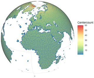
Figure 1 Number of grid cell centers of the longitude–latitude grid that fall into each hexagonal grid cell of the ISEA3H grid at resolution 7. The color pattern shows that closer to the poles, more grid cell centers fall into each hexagonal cell compared to the areas around the Equator.

After mapping the original cell centers into the ISEA3H grids, the mean of all observations within each hexagonal cell is taken as the new value in the transformed data set.

3.3 Area weights

Instead of directly converting the data into the area-preserving ISEA3H grid system, one could alternatively adjust the observations from the longitude–latitude grid by weighting them according to their cell size to account for the area distortion. The weight w_i of grid cell i is then defined as $w_i=\frac{\mathrm{area}\mathrm{of}\mathrm{cell}i}{\mathrm{maximum}\mathrm{cell}\mathrm{area}}$. By including these area weights, observations from larger cells have a greater influence on the statistical model than cells from smaller cells. We use this approach as a comparison to better assess the effectiveness of using traditional area weights to address area distortion, in contrast to the equal-area ISEA3H grid system.

3.4 Random forest

We model the observed variation of irrigation fraction with a set of biophysical and socioeconomic predictor variables using a random forest framework.

A random forest consists of a set of individual decision trees that operate as an ensemble. The method was introduced by Breiman (2001) and is now a widely used machine learning technique because it tends to have high prediction power with little tuning of its parameters. A random forest captures non-linear relationships between the predictor variables and the outcome and is able to deal with imbalanced data, and estimates of variable importance are readily available (Strobl et al., 2009).

Depending on the response variable, the decision trees of the random forest perform either classification or regression, based on a recursive partitioning method. At each step, a decision tree finds the optimal split that minimizes “impurity”, until a stopping criterion is met. Impurity serves as a metric for the homogeneity of the class labels at a particular node within the decision tree. Various methods exist to define the impurity measure. Following Wright and Ziegler (2017), we use the estimated response variance for regression trees and the Gini index for classification trees as measures for impurity. Please find the precise steps in Algorithm 1. Ultimately, the recursive partitioning method repeatedly splits the data into potentially high-dimensional rectangular partitions of the predictor space, choosing those for which the response data are relatively homogeneous (Strobl et al., 2009).

Algorithm 1 Random forest

Given a data set $\mathit{\left\{}\right(x_i,y_i):i=\mathrm{1},\mathrm{\dots },n\mathit{\}}$, where y_i is the ith observed dependent variable and $x_i=(X_{\mathrm{1}},\mathrm{\dots },X_p)$ is a p-dimensional predictor vector.
Step 1. Draw a number of n_tree bootstrap samples sets from the training data set. Each sample is the same size as the training data set. The number n_tree is a tuning parameter, also referred to as the number of trees in the forest.
Step 2. At each node split, a random number of m_try predictors out of all P predictors is considered, i.e., $X_i,i=\mathrm{1},\mathrm{\dots },m_{\mathrm{try}}$, with m_try<P. The number m_try is another tuning parameter.
Step 3. Predictor j splits the observations $\mathit{\left\{}{y}_i\mathit{\right\}},i=\mathrm{1},\mathrm{\dots },n$ into the most uniform binary regions $R_l:=\mathit{\{}X\mathrm{|}{X}_j\le c\mathit{\}}$ and $R_{\mathrm{r}}:=\mathit{\{}X\mathrm{|}{X}_j>c\mathit{\}}$ according to the following impurity measures:

• (regression) weighted residual sums of squares

  $$\begin{array}{}\text{(1)}& \begin{array}{rl}{\min }_{j,\mathrm{c}}& \left(p\left(R_{\mathrm{l}}\right)\sum _{j:y_j\in R_{\mathrm{l}}}{\left(y_j-{\stackrel{\mathrm{‾}}{y}}_{R_{\mathrm{l}}}\right)}^{\mathrm{2}}+p\left(R_{\mathrm{r}}\right)\sum _{j:y_j\in R_{\mathrm{r}}}\right.\\ & \left.{\left(y_j-{\stackrel{\mathrm{‾}}{y}}_{R_{\mathrm{r}}}\right)}^{\mathrm{2}}\right),\end{array}\end{array}$$

  where ${\stackrel{\mathrm{‾}}{y}}_{R_{\mathrm{l}}}$ and n_l are the mean and number of observations in region R_l, ${\stackrel{\mathrm{‾}}{y}}_{R_{\mathrm{r}}}$ and n_r are the mean and number of observations in region R_r, and $p\left(R_k\right)=n_k/n$ is the proportion of observations in region $k\in \mathit{\{}l,r\mathit{\}}$,

• (classification) Gini impurity

  $$\begin{array}{}\text{(2)}& {\min }_{j,\mathrm{c}}\left(n_{\mathrm{l}}{\widehat{p}}_{\mathrm{l}}\left(\mathrm{1}-{\widehat{p}}_{\mathrm{l}}\right)+n_{\mathrm{r}}{\widehat{p}}_{\mathrm{r}}\left(\mathrm{1}-\widehat{p_{\mathrm{r}}}\right)\right),\end{array}$$

  where ${\widehat{p}}_k$ is the proportion of sample points that were sent to node $k\in \mathit{\{}l,r\mathit{\}}$ from the previous node.

Step 4. Repeat steps 2–3 until each terminal node reaches the predefined minimum number of observations, min.node.size.
Output. The algorithm forms a partition of the data into M regions $R_{\mathrm{1}},\mathrm{\dots },R_{\mathrm{M}}$, and the response is modeled as a constant r_m, i.e.,

$$\begin{array}{}\text{(3)}& f_{\mathrm{RF}}\left(x\right)=\sum _{m=\mathrm{1}}^{\mathrm{M}}{r}_{\mathrm{m}}I\left(x\in R_{\mathrm{m}}\right).\end{array}$$

A random forest typically consists of several hundreds or thousands of trees and combines the results of their predictions (Strobl et al., 2009). These trees are constructed using bootstrapped samples from the training data, with each sample containing, on average, 63.2 % unique observations (Breiman, 2001), known as in-bag samples. Samples not selected are called out-of-bag (OOB) samples and are used to estimate the prediction accuracy, also called “OOB error”. These error estimates provide an accurate measurement of the generalization error as they are similar to the results obtained through K-fold cross-validation (Wolpert and Macready, 1996). However, the OOB error can be sensitive to the number of random predictors used at each split (m_try) and the number of trees (n_tree) in the random forest (Huang and Boutros, 2016). Generally, the accuracy increases as the number of trees increases. However, the accuracy may level off at a certain number of trees, depending on the specific learning task (Oshiro et al., 2012). The m_try parameter has been found to have a high influence on prediction accuracy and should be selected carefully (Huang and Boutros, 2016; Bernard et al., 2009; Probst et al., 2019). We focus on n_tree and m_try as tuning parameters to achieve a high performing random forest model.

The step-by-step process of building a classification and regression random forest follows Algorithm 1. To cope with the imbalance of our dependent variable, we train two random forests and construct a hurdle model. A classification random forest predicts whether a grid cell is irrigated or not, while a regression random forest predicts the magnitude of irrigation. These models are then combined to create a stacked final model that predicts the irrigation fraction based on the available predictors. This approach effectively handles the zero-inflated distribution of the irrigation fraction.

We use the freely available R package ranger, developed by Wright and Ziegler (2017) for the training and validation of the random forests.

3.4.1 Parameter tuning and model setup

We use cross-validation (CV) to tune our random forest models and determine the values for n_tree (number of decision trees) and m_try (number of predictors to be considered at each split) that maximize predictive accuracy. Data from 1902 to 1999 serve as the training sample, data from 2001 to 2005 are used for validation, and data from 2000 act as test sample. Due to computational constraints, we apply a sub-sampling routine to identify our model parameter values efficiently. For the classification random forests, we draw a balanced sample of 10  in each CV fold, consisting of 50 % irrigated and 50 % rainfed grid cells. This is achieved using random over- and under-sampling methods from the R package ROSE, provided by Lunardon et al. (2014). For the regression random forest, all irrigated grid cells are used for training.

We use the OOB error and the validation error as accuracy measures. We set the minimal number of data points at each terminal node of min.node.size to 10, serving as a stopping criterion. For the parameter n_tree, we consider the values 50, 300, 500, 800, 1000, 2000, 3000, 4000, and 5000. For m_try we test all values between 1 and 5 at 0.5 increments for both the classification and regression random forests. We conduct 50-fold CV to train the classification and regression random forests separately for each grid choice.

The resulting accuracy for each forest and each tuning parameter value can be seen in Figs. S3 and S4. Taking the OOB error and the validation error into account, we choose n_tree=1000 and m_try=1.5 for the classification random forest and n_tree=4000 and m_try=5 for the regression random forest for the longitude–latitude grid. In the ISEA3H grid we set n_tree=1000 and m_try=5 for the classification random forest and n_tree=4000 and m_try=5 for the regression random forest.

After setting the tuning parameters, we evaluate the prediction accuracy of the stacked random forest model on the test data. The final model prediction is obtained by multiplying the predictions from the classification random forest by those from the regression random forest.

We then compare the final prediction results for models build on the original longitude–latitude grid; the longitude–latitude grid using area weighting; and the ISEA3H grids at resolutions 7, 8, and 9.

4 Results and discussion

4.1 Grid choice

We compare the longitude–latitude grid to the ISEA3H grids based on their predictive power and their ability to identify the drivers of the global irrigation expansion. To get a first intuition about differences in predictive power, we create binned scatter plots of the predicted irrigation fraction of the test data against the observed values of irrigation fraction for all grid choices. In that way, the 45° line mechanically indicates correctly predicted irrigation fraction values. Figure 2 shows the results. The comparison suggests that the ISEA3H grid models at resolution 7 and 8 have a higher prediction accuracy, since the point values scatter more closely around the 45° line. This could be due to the fact that at resolutions 7 and 8, the grid cells are larger, and therefore the value of the dependent variable is less nuanced. There is no clear visual difference between the predictive accuracy of the longitude–latitude grid and the ISEA3H grid at resolution 9.

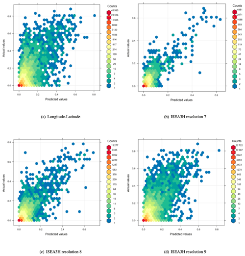
Figure 2 Binned scatter plot of predicted vs. observed irrigation fraction values. The prediction is based on the test data.

To further evaluate the difference in predictive accuracy between grid choices, we compute the root mean square error (RMSE) and the normalized root mean square error (NRMSE) as

$$\begin{array}{}\text{(4)}& \mathrm{RMSE}=\sqrt{\mathrm{1}/n\sum _{i=\mathrm{1}}^n{\left(y_i-\widehat{y_i}\right)}^{\mathrm{2}}}\end{array}$$

and

$$\begin{array}{}\text{(5)}& \mathrm{NRMSE}={\displaystyle \frac{\mathrm{RMSE}}{\mathrm{SD}\left(y\right)}},\end{array}$$

where y_i is the observed value, ${\widehat{y}}_i$ the prediction, and SD(y) the standard deviation over all observed values. The RMSE and NRMSE were calculated for the prediction on the test data and compared between grid choices. We additionally evaluate the NRMSE, after restricting the sample to observations with non-zero irrigation. The outcomes are reported in Table 2. The model with the lower NRMSE is considered the better choice to model irrigation fraction.

Table 2 Normalized root mean square error comparison between grid choices.

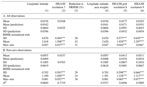
Column 1 shows the mean and standard deviation of the irrigation fraction and the NRMSE values of the longitude–latitude grid choice. Column 2 provides the same for the ISEA3H grid resolution 7 choice. In column 3 the reduction in NRMSE is documented in percent and in comparison to the longitude–latitude grid. Column 4 presents the result for a model based on the longitude–latitude grid with additional area weights, and columns 5 and 6 provide the results for the ISEA3H resolution-8 and resolution-9 grids. Panel A. includes all observations and gives the overall NRMSE estimates. In Panel B. only irrigated areas are included. The NRMSE values provide insight into how the models perform on actually irrigated terrain. ^*, ${}^{**}$, and ${}^{***}$ indicate 10 %, 5 %, and 1 % significance for the t test of difference in bootstrapped mean NRMSE values with 500 repetitions, comparing the ISEA3H models (columns 2, 5, and 6) with the longitude–latitude model (column 1).

To verify the robustness of our result, we calculate the NRMSE using the mean and the distance between the minimum and the maximum value as standardizing measures.

In order to investigate the robustness of our error measure, we implement a bootstrapping analysis, in which we generate each model in 500 repetitions and predict irrigation fraction using a random 40 % sample of the test data in each step. We then calculate the difference in NRMSE values between the longitude–latitude benchmark model and the other specifications. By examining the distribution of these differences, we are able to assess whether observed differences are statistically significant.

Additionally, we include a model based on the longitude–latitude grid with traditional area weights. This allows us to assess the effectiveness of using area weights to address area distortion as compared to the equal-area ISEA3H grid.

Generally, we see that lower errors are observed when using an ISEA3H grid. For all observations, the ISEA3H resolution-7 grid exhibits a 28 % reduction in NRMSE compared to the longitude–latitude grid, with a value of 0.484 compared to 0.676. The ISEA3H grids at resolutions 8 and 9 also show improved performance over the longitude–latitude grid, with NRMSE values of 0.577 and 0.645, respectively. The longitude–latitude grid with area weights does not significantly improve the NRMSE compared to the standard longitude–latitude grid.

Focusing on irrigated areas, the ISEA3H resolution-7 grid demonstrates a 29 % lower NRMSE (0.503) compared to the longitude–latitude grid (0.702). Similar trends are observed for the ISEA3H grids at resolutions 8 and 9, with NRMSE values of 0.598 and 0.666, respectively. Again, the longitude–latitude grid with area weights shows marginal or no improvement.

This trend remains consistent across all normalization specifications, which emphasizes the comparative performance of the ISEA3H grid choices and their advantages over traditional longitude–latitude grids.

In a next step, we consider predicted irrigation fraction. We evaluate how accurately the models predict high and low values of irrigation fraction across the globe. Figure 3 shows the difference between predicted irrigation fraction and observed irrigation fraction for all grid choices. The computation is based on the test data. The color scale indicates if the model predicts the irrigation fraction accurately or suffers from under- or over-prediction. Yellow areas are correctly predicted by the model, orange to red areas correspond to under-prediction, and green to blue areas indicate over-predicted irrigation fractions. Considering the longitude–latitude grid, we see that irrigation is under-predicted in some areas in India and east Asia and also in a few areas in North and South America and Europe. Except for a very few parts in India, central Africa, and North America, we do not see any over-prediction of irrigation. Looking at the ISEA3H grids, we find that the same areas in India and east Asia are slightly over-predicted as well as some areas in the United States and Europe. Only a few areas are under-predicted in India, east Asia, and central Africa. Comparing both grid systems, we find that the ISEA3H grids are closer to the original irrigation pattern in all areas. In particular, the highly irrigated areas in east Asia are better captured by the ISEA3H grid models, and we also see less over-prediction in European areas. The maps indicate that the ISEA3H grid system is the better choice in predicting the global irrigation fraction pattern.

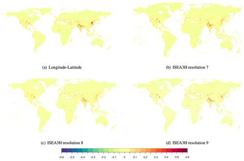
Figure 3 Deviation of the predicted irrigation fraction from the observed irrigation fraction in (a) the longitude–latitude grid and (b–d) the ISEA3H grids at resolutions 7, 8, and 9. Green and blue areas indicate under-prediction of the irrigation value, and orange and red values over-prediction. Yellow areas correspond to areas where irrigation values were predicted correctly. The prediction is based on the test data.

4.2 Drivers of irrigation expansion

4.2.1 Variable importance

We report the importance of the predictors for both the classification random forests, which predict the probability of irrigation occurring, and the regression random forests, which predict irrigation magnitude given that the area is irrigated. In the classification random forests, relative importance is measured by Gini gain, while in the regression random forests, it is captured by the estimated response variance. The results are displayed in Fig. 4.

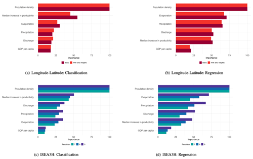
Figure 4 Relative importance, measured as decrease in node impurity. The results for the longitude–latitude grids can be seen in red, and the results for the ISEA3H grids are displayed in blue. The order of variables in the importance plots is robust to 500 bootstrap steps.

The most important driver for the probability that an area is irrigated is population density. This is the case for all grid choices. The second-most-important driver is the median potential increase in productivity in terms of crop yield. Evaporation, precipitation, and discharge all have a similar influence on irrigation probability. However, the order of importance is reversed between the two grid choices. GDP per capita only has a small influence on the decision to irrigate.

The most important driver of irrigation intensity, given that an area is already irrigated, is also population density. This is followed by evaporation, precipitation, discharge, and a median increase in potential productivity, where the order of discharge and median potential productivity increase is reversed for the ISEA3H grids. The least important driver is again GDP per capita, though it still has some influence on the models' performance in all grids.

Looking at the different patterns across resolutions, it appears that finer resolutions increase the relative influence of predictors other than population density. This makes sense, as these other drivers likely have a greater impact at a local level, whereas population density reflects a broader need for crop production in the area.

4.2.2 Partial dependence

We compute the partial dependence of each predictor variable for all grid choices and model specifications. The partial dependence is obtained by gradually changing the value of one predictor variable and predicting the outcome variable at each step, while leaving the remaining predictors constant. That way, the functional relationship between the predictor and the dependent variable becomes visible. The larger the value range on the vertical axis, the larger the influence of the predictor on the dependent variable. Figure 5 illustrates the results.

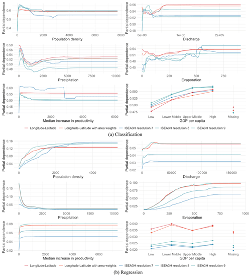
Figure 5 Partial dependence of the predictors and the dependent variable of (a) the classification random forests and (b) the regression random forests. The results for the ISEA3H grids (resolution 7, 8, and 9) are shown in shades of blue, and the results for the longitude–latitude grid and the model with area weights are shown in red.

Figure 5a illustrates the partial dependence of the predictors of irrigation probability. Overall, we see very intuitive dependence patterns. Population density has a positive influence on the probability to irrigate, where the probability sharply increases at the beginning of the population density distribution. In other words, greater population density correlates with an increased probability of irrigation, indicating that metropolitan regions with higher population densities and improved market accessibility are more likely to engage in irrigation. This heightened probability is likely attributed to the requirement of capital investment for establishing irrigation systems. This aligns with the paper by Neumann et al. (2011), who also found a positive association between irrigation and population density.

A similar pattern can be seen for the median potential increase in productivity, the second-most-influential predictor. The positive correlation demonstrates that the potential increase in crop yield is a factor for the decision to implement irrigation systems.

Evaporation also has a positive, almost linearly increasing influence on irrigation probability. Considering precipitation, our results show that the probability to irrigate decreases with the amount of precipitation until the probability levels off. The amount of available discharge has a negative relationship with the probability to irrigate for both grid choices at the beginning of the distribution. Looking at the longitude–latitude grid, this changes into a positive correlation, leaving us with a u-shaped dependence curve. Looking at the ISEA3H grid choice, the irrigation probability does not change anymore after reaching a certain discharge level. Overall, these results show that water availability and climatic conditions play a role in the decision to irrigate, leaving rather dry areas and areas with higher evaporation levels more likely to be or become irrigated. Discharge is an accumulated variable of local runoff, with very high differences between upstream and downstream cells in a watershed. This means that regions with relatively high topography and thus potentially lower degrees of agriculture and irrigation are all coinciding with low discharge values, while the major irrigation areas (India, Pakistan, United States, east Asia, Egypt, etc.) generally lie close to large streams with high discharge. The correlation with elevation might explain why initially the dependence of irrigation on discharge decreases. For large values the large grid size might be able to explain the differences between the grids; for example, along the Nile the irrigated areas follow the river in a small band, being dispersed in the ISEA3H grid.

Lastly, we study the GDP-per-capita categories as a function of the probability of observing irrigation. We find a strictly positive relationship from the categories “low”, “lower middle”, and “upper middle” to “high”. Therefore, the likelihood of croplands being irrigated is higher for areas with generally higher economic performance. Hence, adverse socio-economic conditions hinder the development of irrigated agriculture. This result complements the findings of Neumann et al. (2011), who found similar effects considering government performance and government type. The GDP-per-capita category “missing” corresponds to a relatively lower irrigation probability. This is in line with the fact that in earlier time periods, fewer areas were irrigated, and more GDP-per-capita observations were missing.

Figure 5b displays the partial dependence curves for the predictor variables of irrigation intensity, i.e., the amount of irrigation given a grid cell is irrigated. The most influential predictor, population density, positively impacts the amount of irrigation.

Evaporation is also positively associated with the amount of irrigation, where the increase in irrigation appears to be almost linear in evaporation levels. The amount of irrigation negatively depends on precipitation levels, while discharge is positively correlated with irrigation intensity. Hence, the effect of water availability differs between different sources of water, where heavily precipitated areas do not seem to require as much irrigation, while discharge might be used to feed irrigation systems.

The median potential productivity gain is positively associated with irrigation intensity, exhibiting a sharp peak in the dependence curve at the beginning of the distribution. A large part of the tail is probably irrelevant for a real-world scenario, where irrigation would never happen in remote and dry regions, with a high potential for productivity increases from irrigation. Larger cell sizes in the ISEA3H grid mean “easier” access to streams (more area is in the same cell as the river), which is reflected in the higher plateau level.

Considering GDP per capita, we see irrigation intensity only slightly differing between the categories.

Assessing our results in the context of our hypotheses (see Table 1), we generally observe a consistent alignment between our empirical results and our previous theoretical consideration.

5 Conclusions

The careful choice of a discrete global grid system holds significant importance for conducting statistical analyses on a global scale. In this paper, we make use of historical global irrigation data from the last century, to compare the standard longitude–latitude grid to ISEA3H discrete global grids at different resolutions. We employ a stacked random forest framework to model probability of irrigation and irrigation magnitude (once an area is irrigated) as a function of potential drivers. We identify population density and the potential productivity increase in terms of crop yield as the most influential factors for the decision to irrigate and population density and factors accounting for water availability as drivers for intense irrigation. We further point to GDP per capita as having some influence on irrigation behavior.

Comparing the two grid systems, we find that ISEA3H geodesic discrete global grids yield higher prediction accuracies. Using the assigned test data, the model built on the geodesic discrete global grid at resolution 7 produces a 28 % lower normalized root mean square prediction error compared to the model built on the longitude–latitude grid. Although the difference in predictive accuracy decreases with higher resolutions, the ISEA3H grids at resolutions 8 and 9 still produce significantly lower error values compared to the benchmark model. In comparison, using traditional area weights in the longitude–latitude grid does improve prediction accuracy significantly. These results are robust to different normalization definitions.

In terms of the global irrigation prediction pattern, we find that the models based on the ISEA3H grids come closer to the observed irrigation map. While the longitude–latitude grid leads to some highly under-predicted areas in India, east Asia, and the United States, the ISEA3H grids are associated with under-prediction in almost the same areas, although smaller in magnitude. Although the increase in predictive accuracy might partly be due to the fact that the change in grid cell structure changes the scale and therefore the range of values of the targeted irrigation variable, the advantages of the uniformly structured ISEA3H grids are evident and should be explored and tested in future research.

While the combination of water availability, climate, and socioeconomic data offers valuable insights into the role of discrete global grid choice and the drivers of historical irrigation expansion, it is clear that our setting does not come without limitations. For example, we neglected seasonality, meaning that yearly values were used for the analysis. However in reality water availability is much more relevant in the growing season than in the offseason. While we offer new evidence about the potential accuracy increase using a geodesic discrete global grid, our methodology does not include an exhaustive search for the best-possible grid choice. Our goal is rather to set a first reference point for future research designs.

We model irrigation fraction as a function of precipitation, discharge, evaporation, population density, potential productivity increase in terms of crop yield, and GDP per capita. While these are important drivers of irrigation, there are likely other contributing factors that we are not able to capture in our analysis, such as the access to groundwater, irrigation subsidies, or other socioeconomic factors such as the type of government. The access to spatially explicit information would allow researchers to further explore these potential drivers.

Another interesting avenue for future research is to include time lags in the analysis. It might not be the data of the same year (e.g., 1990) that are most indicative of the irrigation fraction of that year but, for example, the (average) data of the previous decade. These time lags might even be different for different predictors.

Lastly, the irrigation and predictor data are based on a large variety of sources from different years, which have likely introduced uncertainties.

Acknowledging these limitations, we consider our analysis an important step towards understanding the role of discrete global grids in global statistical modeling. Particularly, exploring the application of the ISEA3H geodesic grid system in different global analytical contexts presents an intriguing avenue for future research.

Appendix A

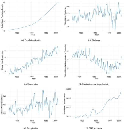
Figure A1 Evolution of the global means of the predictor variables across the study period 1902 to 2005.

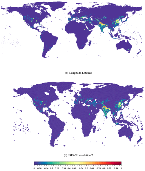
Figure A2 Irrigation fraction in 2000 in (a) the longitude–latitude discrete global grid and (b) the ISEA3H (resolution-7) discrete global grid. Irrigation fraction reflects the area irrigated of each grid cell and is based on the global Historical Irrigation Dataset (see Siebert et al., 2015).

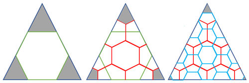
Figure A3 Recursive partitioning aperture-3 method. The hexagonal pattern is recursively constructed on top of the base icosahedron. The first resolution is illustrated by the green hexagon, directly constructed inside a triangular face of the base icosahedron. The construction of the resolution-2 grid is displayed in red in the middle. The resolution-3 hexagonal pattern is illustrated on the right side. Increasing the resolution by 1 leads to hexagons with a size that is one-third of the original hexagon size. The grey leftover areas are the reason that, overall, a few pentagonal faces are needed to cover the Earth's surface. The image is based on an illustration by de Wiljes (2015).

Table A1 Summary statistics of the training data (1902–1999).

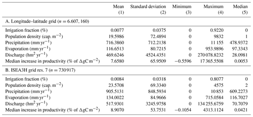
Panel A. summarizes the descriptive statistics of the test data set in the original longitude–latitude grid. The test data set contains the years 1902 to 1999. Panel B. summarizes the descriptive statistics of the ISEA3H grid, i.e., after transforming the data to the hexagonal grid. The GDP-per-capita predictor is excluded from this summary table, as it is a factor variable.

Table A2 Pearson correlation coefficient.

In this table, the correlation matrix of the Pearson correlation coefficient of the predictors is presented. The displayed values are the lower half of the correlation matrix.

Table A3 Variance inflation factor.

This table displays the variance inflation factor (VIF) of the predictor variables. The measure is used to detect multicollinearity between potential predictor variables. A VIF below 5 means that the respective variable is not collinear to the other variables (James et al., 2013).