How to account for irrigation withdrawals in a watershed model

In agricultural areas, the downstream flow can be highly influenced by human activities during low-flow periods, especially during dam releases and irrigation withdrawals. Irrigation is indeed the major use of freshwater in the world. This study aims at precisely taking these factors into account in a watershed model. The Soil and Water Assessment Tool (SWAT+) agro-hydrological model was chosen for its capacity to model crop dynamics and management. Two different crop models were compared in terms of their ability to estimate water needs and actual irrigation. The first crop model is based on air temperature as the main determining factor for growth, whereas the second relies on high-resolution data from the Sentinel-2 satellite to monitor plant growth. Both are applied at the plot scale in a watershed of 800 km² that is characterized by irrigation withdrawals. Results show that including remote sensing data leads to more realistic modeled emergence dates for summer crops. However, both approaches have proven to be able to reproduce the evolution of daily irrigation withdrawals throughout the year. As a result, both approaches allowed us to simulate the downstream flow with a good daily accuracy, especially during low-flow periods.

1 Introduction

The water cycle is substantially affected by climate change. The scientific consortium World Weather Attribution has shown that the 2022 climatic and agricultural drought in Europe would have been about 5 times less likely to happen in the 1900s, and the frequency of such drought will increase further in the coming years. This 2022 drought event has been triggered not only by heatwaves but also by a lack of soil water storage (Schumacher et al., 2022). Many regions suffer from water scarcity, inducing some conflicts between users. Water demands for drinking water and irrigation are, in addition, expected to increase due to population growth. Water management during low-flow periods will therefore be one of the major challenges in future years. Agriculture currently accounts for about 70 % of withdrawals in the world (UNESCO, 2015). In this context, it is important to better assess water needs for agriculture. Efficient tools are then needed to better know the cultivation practices, including irrigated areas, crop dynamics and irrigation practices. These parameters must be assessed in terms of the spatial extents relevant for water management, such as at the river basin or sub-basin scale.

Watershed models are already used by multiple actors on multiple timescales and to different spatial extents. Combined with climate change scenarios, they allow a better understanding of the upcoming challenges for the next decades. For instance, the Explore2070 project (Carroget et al., 2017) has shown with high confidence that the summer streamflow in France in the years 2050–2070 will be, on average, 30 % to 70 % lower than during the years 1990–2010. Combined with management scenarios, watershed models can support decision making for agricultural policies (Murgue et al., 2014; Allain et al., 2018). Furthermore, dam managers and local authorities can make use of short-term forecasts to optimize the low-flow management (E-tiage software: https://www.e-tiage.com/, last access: 9 October 2022; PREMHYCE platform https://webgr.inrae.fr/projets/projets-en-cours/onema-premhyce/, last access: 18 October 2022; Nicolle et al., 2020). Hence the need for continuous improvement of these models.

However, most studies at the watershed scale do not precisely include human activities, especially withdrawals for irrigation. For instance, most users of the SWAT (Soil and Water Assessment Tool) model do not explicitly include withdrawals in their studies (Fohrer et al., 2014; Boithias et al., 2014; Martin et al., 2016; Cakir et al., 2020). In such studies, dam releases and withdrawals are indirectly taken into account through the calibration performed to fit the downstream flow. As a result, the performance of low-flow simulation is quite low, as highlighted by Boithias et al. (2014).

Some modelers include cultivation practices through default crop management or through past years’ statistics, but these models have shown limitations for the prediction of irrigation. Indeed, Leenhardt and Lemaire (2002) describe a case in which the sowing of summer crops was delayed due to the unusually wet spring, but the model did not account for this and predicted the maximum irrigation demand 1 month too early. In the same way, Senthilkumar et al. (2015) highlight the impact of cultivar earliness on their water needs. Models that better fit the actual crops dynamics and management are therefore needed. Remote sensing (RS) offers a real added value for spatial and temporal variability. Since 2016, thanks to the Copernicus program, optical satellite images (Sentinel-2) with high spatial (10 m) and temporal (5 d) resolutions are available anywhere in the world. These resolutions are appropriate to get information on crops dynamics and cultivation practices at the plot scale over a whole watershed.

Methods to retrieve the cultivation practices from RS data have been in development for more than 20 years (Guérif and Duke, 1998; Launay and Guerif, 2005) and have bloomed since short-revisit-time satellites were launched (Courault et al., 2010; Ferrant et al., 2014). The Sentinel constellation, offering a high spatial resolution and high revisit time, has made this task easier and more accurate (Pageot et al., 2020, for irrigated areas; Bazzi et al., 2021, for irrigation events; Rolle et al., 2022, for sowing dates).

For the purpose of water management, RS can also be combined with crop water requirements models. The FAO-56 method (Allen et al., 1998) is the most widely used land surface model in which the potential evapotranspiration (ET) is adjusted with a crop coefficient and a stress coefficient. The classical method uses standard values of crop coefficient, which implies standard growth conditions, but an increasing number of studies replace these with remote sensing data (Saadi et al., 2015; Etchanchu et al., 2017; Battude et al., 2017; Yousaf et al., 2021; Kharrou et al., 2021; Maguire et al., 2022) in order to account for the current-year conditions. In particular, Etchanchu et al. (2017) highlight the contribution of remote sensing data at the plot scale, making more robust calculations of LAI (leaf area index) and ET in comparison to the classical method. In addition to ET calculation, these methods can be used to estimate irrigation through the soil water balance (Saadi et al., 2015; Battude et al., 2017; Kharrou et al., 2021; Maguire et al., 2022) or a comparison with a reference crop coefficient (Yousaf et al., 2021). Even if the retrieval of irrigation suffers from large uncertainties at the farm scale (Saadi et al., 2015, for instance), Olivera-Guerra et al. (2023) have shown that proper calibration can greatly reduce the uncertainties at the irrigation district scale.

Despite these recent advances in the modeling of crop dynamics and water needs, very few works investigate the effect of those cultivation practices on streamflow at high spatial and temporal scales. The MAELIA platform (Modelling of socio-Agro-Ecological system for Landscape Integrated Assessment, Murgue et al., 2014) appears as an exception since it combines the SWAT hydrological model with an agent-based model to perform dam operation and crop management. In this case, modelers have inferred a large set of decision rules either from surveys (Leenhardt et al., 2004; Maton et al., 2005, 2007; Murgue et al., 2014) or from a farm advisor (Clavel et al., 2011). The authors were able to check the relevance of the annual irrigation amount predicted by the model but not the timing of irrigation due to the lack of daily data. The present study intents to go further than the MAELIA project in terms of spatialization by substituting part of the decision rules with remote sensing estimates. Indeed, feeding the model with observations could improve its robustness while avoiding the complexity of an agent-based model.

Some studies already aimed to assess the benefits of optical remote sensing in agro-hydrological models without focusing on crop irrigation. They intended to improve the ET component of the water balance by forcing (Martin et al., 2016; Paul et al., 2021; Jin et al., 2022, all in SWAT model) or assimilating (Kumar et al., 2019, in Noah-MP model; Mohammadi Igder et al., 2022, in SWAT+ model) the RS LAI (remote sensing leaf area index) in the model and short-cutting the plant growth algorithm. Under temperate or arid climate types, ET indeed appears to be the main component of the water balance; hence, a small relative error in ET could lead to a larger relative error in the river discharge. However, even if these authors report an improvement in the yield or carbon fluxes, they report little modification to the streamflow, ranging from 2 % to 7 %. Explanations for these results could be that the modeled LAI, even if uncertain, is enough to compute ET or that the uncertainties in other hydrological or anthropogenic fluxes are larger than the one in ET. As Paul et al. (2021) and Jin et al. (2022) both performed calibrations with and without remote sensing data, this also raises the following question: can calibration correct the errors in ET values in a way that it hides the possible benefits of RS data? Moreover, as far as we know, no studies at the watershed scale used remote sensing data at the plot scale, even though Sentinel data would be suitable for that.

The objective of this study is to take into account human activity during low-flow periods in the modeling process of an agricultural watershed. Unlike previous studies, our work is located on a watershed where irrigation has a huge impact on streamflow: in summer, the downstream flow can be 4 times lower than the upstream flow due to withdrawals. To reach this objective, crop models at the plot scale are used to predict crop water requirements and irrigation withdrawals, and the SWAT+ model is used to compute water stocks and fluxes. The native crop growth module of SWAT is compared to a new module that uses Sentinel-2 high-resolution data to compute ET. An innovative calibration method for hydrological fluxes is introduced to address several calibration issues: the short time depth of Sentinel-2 data, the fact that calibration can hide the possible benefits of RS data, and the highly influenced streamflow. Numerous data sources have been used to carry out the calibration of the irrigation trigger threshold, the estimation of irrigation sources, and the assessment of daily withdrawals. Finally, the relevance of a such model – combining the plot scale and watershed scale during the low-flow period – is assessed.

2 Materials and methods

2.1 Study area

The Gimone watershed (800 km²) has been selected for this study. It is located in southwestern France, in a temperate-climate zone. (Fig. 1). The average rainfall is 700 mm. The flow rate at the outlet ranges from 0.4 to 40 m³ s⁻¹, with an average of 3 m³ s⁻¹. Agricultural land is dominant (85 %) in this watershed. Irrigated crops (mainly corn, soybean, orchards and vegetables) represent about 10 % to 15 % of the total area, and irrigation water is withdrawn from rivers and from individual reservoirs. Other crops, mainly winter wheat, winter rapeseed and sunflower, are not irrigated. Due to the high water demand and low water availability in summer, two dams were built upstream in the 1990s on the Gimone and Marcaoué rivers, with capacities, of respectively, 24 and 1.5 Mm³ (Fig. 1e). The biggest dam is filled with water diverted from the Neste river. Both dams are managed by the CACG (Compagnie d’Aménagement des Côteaux de Gascogne), and their purpose is to maintain a minimal flow rate in rivers during low-flow periods (DOE – Débit Objectif d’Etiage – minimum target flow of 0.4 m³ s⁻¹) and to limit the frequency of irrigation restrictions. As a result, the streamflow during irrigation periods is strongly influenced by dam releases and irrigation withdrawals and has little to do with hydrological processes.

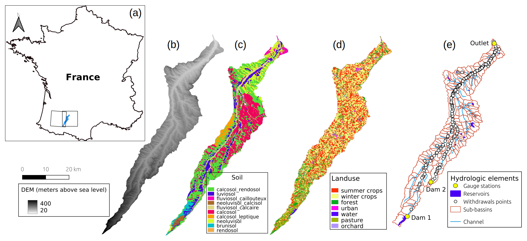
Figure 1 Maps of the study area. (a) Location of the Gimone watershed in southwestern France, as well as Sentinel-2 footprints; (b) digital elevation model (1^′′ resolution); (c) soil map ($\mathrm{1}/\mathrm{250}\mathrm{000}$ resolution); (d) crop pattern for year 2017 (plot scale); (e) hydrological network setup of the model.

2.2 Data overview

The topography of the watershed derives from the SRTM (Shuttle Radar Topography Mission, USGS, 2018) digital elevation model at ∼ 30 m resolution (Fig. 1b). Daily weather data – precipitation, air temperature, wind velocity, solar radiation and air humidity – were extracted from the SAFRAN product (Durand et al., 1993). It is an interpolation based on weather measurements and model reanalysis on a 8 km resolution grid. Soil properties, namely the depth, bulk density and clay and sand content, were found in the French soil map RRP (Référentiel Régional Pédologique – regional reference document for pedology, GisSol, 2014) at $\mathrm{1}/\mathrm{250}\mathrm{000}$ resolution (Fig. 1c); the maximal root depths were set according to Rigou (2016); the available soil water content (AWC) was derived from Bruand et al. (2003) pedotransfer functions; the initial estimate of the saturated hydraulic conductivity comes from measurements. Land use data come from the French database of agricultural land use (RPG – Registre Parcellaire Graphique, IGN, 2021) for the years 2015 to 2021, completed by the OSO map (Inglada et al., 2017) for non-agricultural areas (Fig. 1d) (Inglada et al., 2018). Streamflow coming out of the two dams was provided by the CACG.

In addition to the classical data to set up the SWAT+ model, high-resolution remote sensing data were used. Since 2017, the two Sentinel-2 satellites provide images every 5 d, with resolutions ranging from 10 to 60 m depending on the wavelength (Drusch et al., 2012; ESA, 2012). The level-2A images from two Sentinel-2 tiles, 31TCJ and 30TYP (Fig. 1a), are used in this study. They are post-processed through the MAJA chain (Hagolle et al., 2015) that corrects atmospheric effects and produces a cloud mask. These clouds masks are used in the interpolation process to obtain gap-filled time series.

River discharge at the outlet was also provided by the CACG and has been used for calibration and validation. In order to get an overview of the origin of withdrawals, the PAR (Plan Annuel de Répartition – annual plan for water allocation) database was used. It gathers individual withdrawal permissions issued every year by the French administration and contains the authorized volumes in each type of water resource. The PKGC (Pratiques Culturales en Grandes Cultures – agricultural practices in field crops) database (Agreste, 2020), carried out every 5 years, consists of a large survey that covers all French departments, with information for about 28 000 agricultural plots. The dataset from 2017 has been used in this study, particularly the sowing dates and amounts of annual irrigation of 160 corn and soybean fields in southwestern France.

A large part of the irrigation pumps of the Gimone watershed are equipped with networked meters (Fig. 1e). These provide daily measurement of water withdrawn from the two main rivers, the same two that are regulated with dams and for which low flows are sustained during summer (Gimone and Marcaoué). Not all intake points are equipped for the years considered in the present study: 33 % of the pumps were equipped in 2019, 62 % were equipped in 2020, and 72 % were equipped in 2021. For this reason, only 2020 and 2021 data were used and were corrected with a proportionality coefficient to convert those data into total withdrawals.

2.3 SWAT+ model

2.3.1 Global overview

The Soil and Water Assessment Tool (Arnold et al., 1993, 2012) is a agro-hydrological semi-distributed and process-based model. To set up this semi-distributed approach, the simulated watershed is divided into multiple sub-basins according to topography. Each sub-basin is divided into HRUs (hydrological response units), which are homogeneous areas in terms of slope, soil and land use. Calculation of the process-based water balance is then carried out at the HRU level on a daily basis (Neitsch et al., 2001). Daily rainfall is split between surface runoff and infiltration using the curve number method (Soil Conservation Service, 1972; Rallison and Miller, 1982). Soil water sustains evapotranspiration and leads to subsurface runoff and percolation into aquifers. If the simulated water table of the shallow aquifer is high enough, ground water flow from the aquifer supports river flow. This contribution of aquifers to the river flow is called baseflow. Land use management (e.g., planting, irrigation, fertilization, harvest) occurs on the basis of user-defined decision rules. When irrigation is applied, the origin of withdrawals (river, aquifer, reservoir) must be specified so that the amount can be subtracted from the appropriate source. All fluxes reaching the rivers (surface and subsurface runoff, ground water flow) are aggregated at the sub-basin level and routed through the stream network to the next sub-basin downstream until reaching the watershed outlet.

2.3.2 Model setup

The 60.5.3 version of SWAT+ has been used in this study as the baseline model, to which features and options were added (see “Code availability” section).

The watershed has been divided into 149 sub-basins (Fig. 1). In this study, we forced HRUs to match individual fields in all agricultural land so that using remotely sensed indices at the plot scale would be consistent. This delineation resulted in about 26 000 HRUs. The model was fed with the true crop rotation from 2015 to 2021 according to the French database RPG.

2.4 Two approaches for crop growth and management

Two methods have been compared to simulate crops seasonal dynamics. The first one is the native crop growth module of SWAT, based on a simplified version of EPIC (Erosion Productivity Impact Calculator). The second one consists of observations of measured crop growth through the normalized difference vegetation index (NDVI), a remote-sensing-based index linked to vegetation development. The two approaches are hereafter called SWAT-O and SWAT-NDVI, respectively. The SWAT-O setup has also been run without any irrigation to assess the impact of withdrawals on the streamflow. Below is a short description of both methods.

2.4.1 SWAT-O: growth of plants and ET driven by heat units (EPIC)

Heat units (namely the average temperature of the day minus the base temperature) drive the growth of LAI (leaf area index) according to the following formulas (Barnard, 1948; Phillips, 1950):

$$\begin{array}{}\text{(1)}& {\displaystyle }{\mathrm{fr}}_{\mathrm{LAImx}}={\displaystyle \frac{{\mathrm{fr}}_{\mathrm{PHU}}}{{\mathrm{fr}}_{\mathrm{PHU}}+\exp (l_{\mathrm{1}}-l_{\mathrm{2}}\cdot {\mathrm{fr}}_{\mathrm{PHU}})}},\text{(2)}& {\displaystyle }{\mathrm{fr}}_{\mathrm{PHU}}={\displaystyle \frac{{\sum }_{i=\mathrm{1}}^d{\mathrm{HU}}_i}{\mathrm{PHU}}},\end{array}$$

where fr_LAImx is the fraction of maximum LAI, l₁ and l₂ are shape coefficients, HU_i is the heat unit of day i (^∘C), and PHU is the potential heat unit required for plant maturity (^∘C). A more detailed description of this simplified EPIC module can be found in the SWAT theoretical documentation (Neitsch et al., 2001).

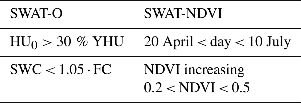
The beginning of growth is settled according to decision rules, where the most important parameter is the sum of heat units since 1 January (HU₀). The emergence occurs on the first day that all the conditions are met. See an example for corn in Table 1.

Table 1 Decision rules for corn emergence. The emergence occurs on the first day that all the conditions are met. YHU: total heat units of the year; SWC: soil water content; FC: field capacity.

Potential evapotranspiration (PET) of the crop depends on its LAI based on Penman–Monteith equation (Monteith, 1965):

$$\begin{array}{}\text{(3)}& {\displaystyle }\mathit{\lambda }{E}_{\mathrm{t}}={\displaystyle \frac{\mathrm{\Delta }(H_{\mathrm{net}}-G)+\mathit{\gamma }{K}_{\mathrm{1}}\cdot (\mathrm{0.622}\mathit{\lambda }\cdot \frac{{\mathit{\rho }}_{\mathrm{air}}}{P})\cdot \frac{e_z^o-e_z}{r_{\mathrm{a}}}}{\mathrm{\Delta }+\mathit{\gamma }\cdot (\mathrm{1}+r_c/r_{\mathrm{a}})}},\text{(4)}& {\displaystyle }{r}_c={\displaystyle \frac{r_l}{\mathrm{0.5}\cdot \mathrm{LAI}}},\end{array}$$

where r_c is the stomatal resistance (s m⁻¹), r_l is the stomatal resistance (s m⁻¹) of a single leaf, E_t is the maximum transpiration (mm d⁻¹), λ is the latent heat of vaporization (MJ kg⁻¹), Δ is the slope of the saturation vapor pressure–temperature curve ($\mathrm{kPa}{}^{\circ }{\mathrm{C}}^{-\mathrm{1}}$), H_net is the net radiation ($\mathrm{MJ}{\mathrm{m}}^{-\mathrm{2}}{\mathrm{d}}^{-\mathrm{1}}$), G is the heat flux density to the ground ($\mathrm{MJ}{\mathrm{m}}^{-\mathrm{2}}{\mathrm{d}}^{-\mathrm{1}}$), γ is the psychometric constant ($\mathrm{kPa}{}^{\circ }{\mathrm{C}}^{-\mathrm{1}}$), ρ_air is the air density (kg m³), P is the air pressure (kPa), K₁ is a dimension coefficient (K₁= 86 400 s d⁻¹), $e_z^o$ is the saturation vapor pressure (kPa), e_z is the vapor pressure of air (kPa), and r_a is the aerodynamic resistance (s m⁻¹).

Actual evapotranspiration is adjusted from this PET through a stress coefficient calculated as follows:

$$\begin{array}{}\text{(5)}& K_{\mathrm{s}}=\left\{\begin{array}{ll}\exp \left(\mathrm{5}\left(\frac{\mathrm{SWC}}{\mathrm{0.25}\cdot Zr\cdot \mathrm{AWC}}-\mathrm{1}\right)\right)& \text{if }\frac{\mathrm{SWC}}{\mathrm{0.25}\cdot Zr\cdot \mathrm{AWC}}<\mathrm{1}\\ \mathrm{1}& \mathrm{else}.\end{array},\right.\end{array}$$

where SWC is the soil water content (mm), and Zr is the root depth (mm).

2.4.2 SWAT-NDVI: growth of plants and ET driven by optical remote sensing

A normalized difference vegetation index (NDVI) is calculated from red and near-infrared (NIR) bands (fourth and eighth bands) of Sentinel-2 and is used as a proxy for vegetation growth:

$$\begin{array}{}\text{(6)}& \mathrm{NDVI}={\displaystyle \frac{\mathrm{NIR}-\mathrm{Red}}{\mathrm{NIR}+\mathrm{Red}}}.\end{array}$$

The bare-soil NDVI is lower than 0.2, whereas the crop NDVI ranges from 0.2 at the early stages to 0.7–0.9 at full development. Table 1 shows the rules used to detect crop emergence with NDVI.

Actual evapotranspiration (E_t, mm) is calculated with the FAO-56 dual-coefficient method (Allen et al., 1998):

$$\begin{array}{}\text{(7)}& E_{\mathrm{t}}=(K_{\mathrm{cb}}\cdot K_{\mathrm{s}}+K_{\mathrm{e}})\cdot E{T}_{\mathrm{0}},\end{array}$$

with ET₀ being the evaporative demand (mm), K_cb being the crop basal coefficient, K_e being the soil evaporative coefficient, and K_s being the stress coefficient. K_cb can be seen as a linear function of NDVI, the coefficients of which were fixed following Toureiro et al. (2017):

$$\begin{array}{}\text{(8)}& K_{\mathrm{cb}}=\mathrm{1.464}\cdot \mathrm{NDVI}-\mathrm{0.253}.\end{array}$$

The K_e factor depends on the crop coefficient K_cb, the fraction of soil coverage F_cover, and a reduction coefficient K_r:

$$\begin{array}{}\text{(9)}& K_{\mathrm{e}}=min\left(K_{\mathrm{r}}\cdot (\mathrm{1.2}-K_{\mathrm{cb}});\mathrm{1.2}\cdot (\mathrm{1}-F_{\mathrm{cover}})\right),\end{array}$$

with

$$\begin{array}{}\text{(10)}& F_{\mathrm{cover}}=\mathrm{1.23}\cdot \mathrm{NDVI}-\mathrm{0.15},\end{array}$$

and K_r depends on the soil texture and SWC according to Merlin et al. (2011).

The stress coefficient is calculated as

$$\begin{array}{}\text{(11)}& K_{\mathrm{s}}={\displaystyle \frac{\mathrm{SWC}}{(\mathrm{1}-p)\cdot Zr\cdot \mathrm{AWC}}},\end{array}$$

where p is the depletion coefficient that is usually equal to 0.55 in the FAO-56.

2.5 Model for irrigation

Based on local water managers' knowledge, all fields with a slope lower than 10 % and that are covered by corn, soybean, orchard or vegetables were considered to be irrigated. The actual source of irrigation withdrawals (river or reservoirs) is not known. The PAR database, however, provides information about the distribution of authorized withdrawals between sources. We assumed the real withdrawal distribution to be the same. It results in 58 % of the water being pumped from the rivers, whereas 42 % comes from small reservoirs (36 % from connected reservoirs and 6 % from disconnected ones). As small reservoirs (< 10 ha) are not included in our setup, irrigation water was considered to come from the closest river in relation to each HRU. This should be kept in mind for the interpretation of results.

Rules are required to trigger the simulated irrigation. In order to implement them, we used several surveys conducted in southwestern France to identify farmers’ behaviors (Leenhardt et al., 2004; Maton et al., 2005, 2007; Senthilkumar et al., 2015). Table 2 presents the implemented rules, which include soil water content, the rainfall of the day and the next day, and crop phenological stages.

Table 2 Decision rules for irrigation of corn. SWC: soil water content; fr_PHU: fraction of YHU.

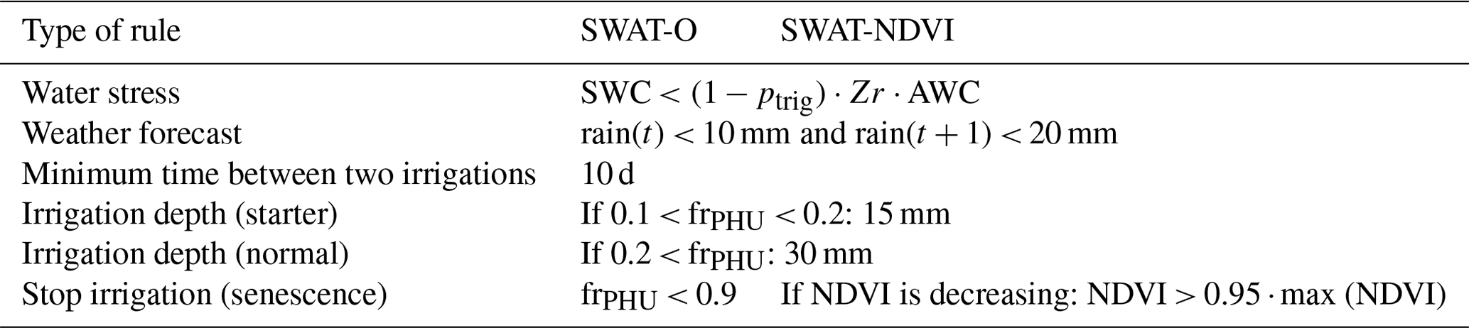
The p_trig parameter (Table 2) can vary depending on the crop, and it was calibrated for corn and soybean. The calibration method is similar to the one described by Olivera-Guerra et al. (2023). Calibration and validation data are the annual irrigation depth for 160 irrigated fields in the PKGC database. This led to a value of 0.57 for corn and soybean and 0.55 for silage corn.

2.6 Calibration of hydrological processes in SWAT

Streamflow in the Gimone River during summer is more impacted by human activities (release of water from dams, withdrawals) than by natural hydrological processes. In order to take this into account, calibration of natural hydrological parameters has been performed for months where anthropogenic impact is reduced: from November to May.

The calibration of parameters related to natural hydrology has been performed only for the SWAT-O setup, and calibrated values were also used for the SWAT-NDVI setup for several reasons. First, Sentinel-2 remote sensing data are only available from 2017. The SWAT-NDVI setup would have not allowed us to cover a sufficiently long period to perform calibration and validation over contrasted hydrological years. This choice has also been made to make a more straightforward comparison between the two crop models. Indeed, if calibration had been performed for both setups, the specificity of each crop model could have been hidden.

The years 2017 to 2021 have been used as the calibration period, and the years 2012 to 2016 have been as the validation period. The years 2010 and 2011 have been run as a warm-up period.

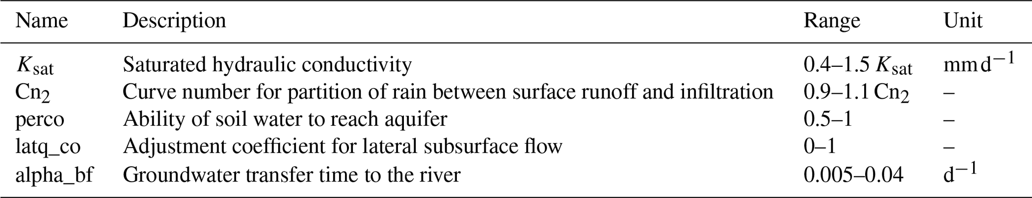
Sensitive parameters have been identified through a sensitivity analysis using a one-at-a-time procedure as described by Abbaspour (2015) and based on a previous study conducted in this watershed (Grusson et al., 2015; Cakir et al., 2020). This allowed us to adjust the range of each parameter before starting the calibration process. The parameters are listed in Table 3.

Table 3 Parameters selected for calibration, as well as the range within which they can vary.

Calibration has been performed by randomly drawing 1000 sets of parameters following a uniform distribution within the tested range of each parameter. The model was then run for each of these 1000 sets over the 2010–2021 period. For each of the 1000 runs, several metrics have been calculated based on daily flow over the 5-year calibration period, excluding June to October. The metrics are the Nash–Sutcliffe efficiency (Nash and Sutcliffe, 1970) performed for the logarithm (NSElog) and the square root (NSEsqrt) of the discharge, as well as the Kling–Gupta efficiency performed for the square root of the discharge (KGEsqrt) (Gupta et al., 2009). The square root (sqrt) and logarithm (log) transforms, respectively, put the emphasis on middle-range and low flows (Pushpalatha et al., 2012; Santos et al., 2018). For each score independently, the top 1 % parameter sets were analyzed using boxplots. The dispersion between those best sets allows us to highlight the equifinality issue during the calibration process.

The goodness of fit of the validation period was then evaluated with the same metrics and additionally with R² and P_bias. Eventually, only NSElog was used to select the parameter values because the calibration months (November to May) still contained low flows but were influenced very little by withdrawals. In order to assess the uncertainty due to calibration, the four best parameter sets according to NSElog were selected for the rest of this study.

3 Results and discussion

3.1 Calibration and hydrology outside the low-water period

Figure 2 shows the dispersion of the top 1 % of sets of parameters according to each criterion independently (NSEsqrt, NSElog, KGEsqrt). Since the bounds of the y axis correspond to the range of each parameter, a low dispersion of values reveals a high sensitivity of the parameter and a low equifinality.

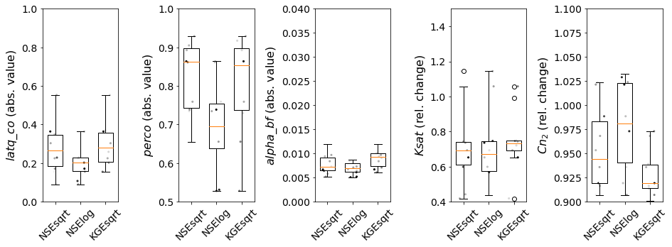
Figure 2 Boxplot analysis of the parameter values of the 10 best simulations according to three different metrics.

Accordingly, alpha_bf and, to a lesser extent, Cn₂ are sensible parameters. A relative value of Cn₂ below 1 means that the runoff-over-infiltration ratio must be lower than the default values. A value of alpha_bf around 0.005 to 0.01 d⁻¹ means that the transfer time from the aquifer to the river is about 3 to 6 months. Although no transfer time measurements are available to check the credibility of this value, the simulated base flow is consistent with the base flow index (BFI) of the river calculated with the Wallingford method (Hamon, 1963; ESPERE software from BRGM: https://www.brgm.fr/fr/logiciel/espere-estimation-pluie-efficace-recharge-selon-differentes-methodes; Lanini et al., 2020).

On the contrary, latq_co and K_sat values seem to be scattered over a wider range. However, further analyses have shown that these parameters are highly correlated because they are both used to calculate the sub-surface lateral flow: if latq_co is low then K_sat must be high and vice versa – hence the conclusion that when the value of one of these two coefficients is fixed then the other becomes very sensitive. Only the perco coefficient seems to have a lower sensitivity.

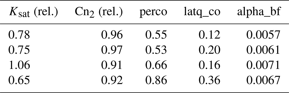
Due to the dispersion of the best parameters without large differences in the scores, it seemed appropriate to keep more than one set of parameters. This allows us to account for calibration uncertainty in future runs. The four bests sets of parameters according to NSElog are therefore kept (Table 4). Table 5 shows the values of metrics during calibration (2017–2021) and validation (2012–2016) periods for the simulation using the first parameter set. It is worth noting that these scores are calculated only over the months of November to May.

Table 4 Four best parameter sets according to NSElog.

Table 5 Calibration and validation scores.

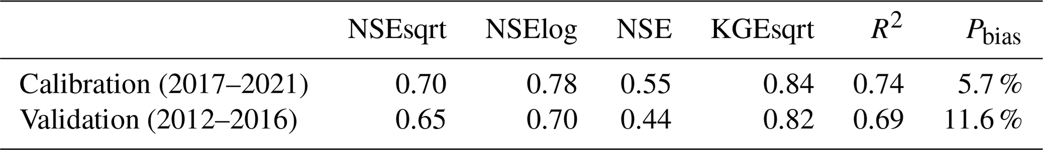
The NSE value is only satisfactory (Moriasi et al., 2007), but since NSE mostly assesses the performance for high flows, which are not the goal of this study, and knowing the limitation of discharge measurement for high flows, these values are seen as sufficient here. On the other hand, the NSElog values and the KGEsqrt values are very good in the calibration period and good in the validation period according to the classification of Moriasi et al. (2007, 2015). This indicates a good agreement for medium and low simulated flow rates compared to measurements. As for R² and P_bias, these values are considered to be good and very good, respectively.

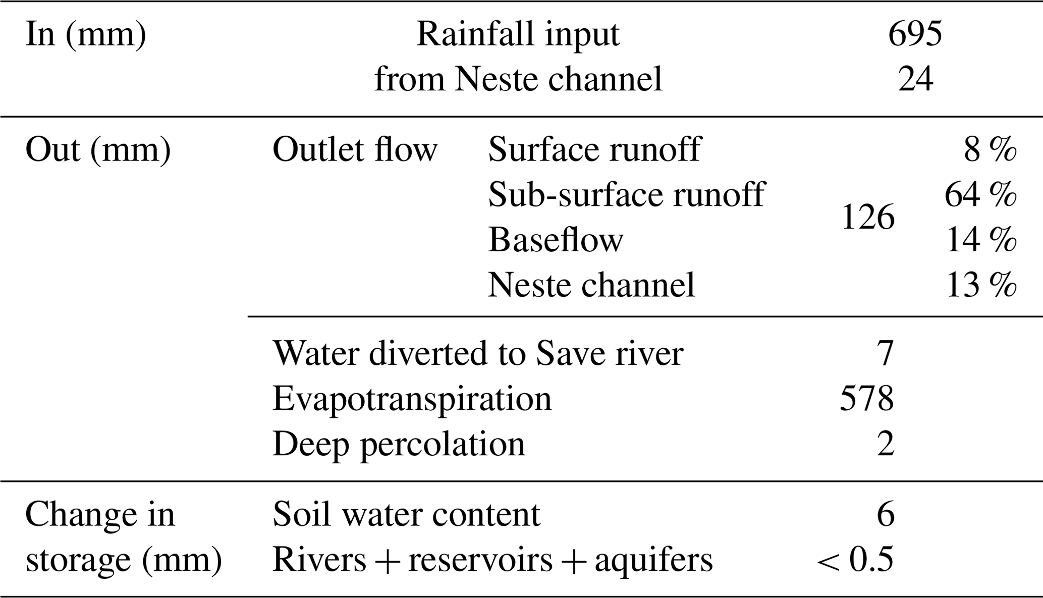
The annual water balance averaged over 10 years (2012–2021) as simulated from the calibrated values is detailed in Table 6. Rainfall (around 700 mm per year) is mostly converted into evapotranspiration (around 580 mm per year) and flow (126 mm per year). In comparison, the measured annual flow is 116 mm per year. In this section of the study, the simulated streamflow is not yet reduced by withdrawals, which can explain most of the difference. This water balance is very similar to the one obtained by Boithias et al. (2014) in a nearby and similar watershed. By not including human influence on the streamflow, they reported a way lower performance in low-flow periods compared to in high-flow periods. This is the reason why our hydrological calibration is performed only during the November–May period, whereas the influenced flow (June–October) performance is investigated in the following sections. Table 6 also shows that two-thirds of the river flow comes from subsurface runoff. Baseflow accounts for about 14 % of the total flow.

Table 6 Annual water balance from the calibrated SWAT model, averaged over the years 2012–2021, and streamflow separation.

The daily calibrated streamflow at the outlet is shown in Fig. 3. The four simulations with the four selected sets of parameters are plotted as a minimum–maximum colored range, along with a plain line for the median value.

3.2 Plant phenology

The emergence of crops follows the rules described in Sect. 2.4. As a result, the emergence dates have very different distributions depending on the method. In the SWAT-O setup, most of the crop growths are synchronized. For instance, in 2017, the model grows all corn during the last week of May. The reason is that the growth in SWAT-O is mostly determined by air temperature, which is nearly homogeneous over the watershed. On the other hand, the use of NDVI to detect the beginning of growth spreads the emergence dates over almost 2 months. Figure 4 shows this effect on the 700 corn fields in the Gimone watershed. To decide which distribution is the more realistic one, those dates have been compared to 150 corn fields from the PKGC database located within 80 km of the study area. The assumption is made that the dynamics of these plots and of the Gimone plots are similar due to the similarity in the altitudes, latitudes and climate. The PKGC database contains the sowing date, whereas the use of NDVI allows the detection of the phenological stages 6 to 8 of leaves (hereafter called emergence for more clarity). For consistency between NDVI and PKGC estimations, a fixed amount of 300 heat units has been added to the database of sowing dates to be converted into plausible emergence dates, 300 ^∘C d⁻¹ being the average needed to reach the phenological stages 6 to 8 of leaves from sowing.

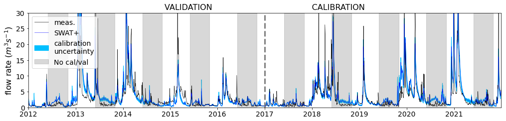
Figure 3 Daily measured and simulated outlet streamflow. Gray areas highlight the periods removed from the calibration–validation process.

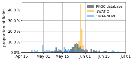
Figure 4 Distribution of corn emergence dates for the year 2017. Comparison between SWAT-O and SWAT-NDVI modes against the reconstructed emergence dates from PKGC database.

Comparison between the PKGC database and the models clearly shows that spread emergence dates (SWAT-NDVI) fit better to real dates. Surveys conducted in another sub-watershed in southwestern France in 2005 also showed a spread of sowing dates over 5 weeks (Maton et al., 2007). However, the distribution of emergence dates in SWAT-NDVI does not perfectly match the PKGC distribution either. The major explanation might be the lack of cloud-free Sentinel-2 images during the months of April to June. In 2017, only four dates were usable: 6 April, 16 and 26 May, and 25 June. As images were not available for 40 d, the linear interpolation may lead to unrealistic NDVI time series. In addition, decision rules leads to some artifacts. The peak on 30 April is produced by a lot of plots that already fulfilled the condition of NDVI and that reached the condition of soil water content on the same day in the model. Even if the retrieved emergence dates in the SWAT-NDVI mode were closer to reality, the PKGC date could also not be a representative sample of the diversity of plots. As a consequence, the above comparison focuses on the range of emergence dates without a quantitative description of the distributions.

3.3 Evapotranspiration

Figure 5 shows the monthly simulated ET for the years 2017 to 2021. Both setups lead to quite similar ET, with a monthly average difference of 5 % and a daily average difference of 17 % at the watershed scale. On average, over the 5 years, ET simulated with SWAT-NDVI setup was slightly lower than that in the SWAT-O setup (by 1.5 %).

Figure 5 Monthly evapotranspiration in both setups.

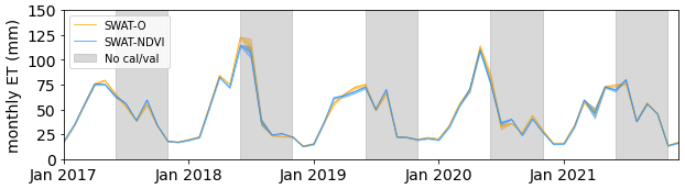
These low differences are in line with the findings of Martin et al. (2016), who also tested the influence of emergence dates retrieved with RS on the water balance. They reported a change in ET from 0 % to ±5 % depending on the months. Their biggest monthly change (around 10 %) occurred in one year where the actual growth of crops was far ahead of the theoretical growth calendar. In the present study, however, no year stands out in particular.

3.4 Daily withdrawals

Figure 6 provides a daily comparison between the simulated water withdrawals and those that are measured by the networked water meters.

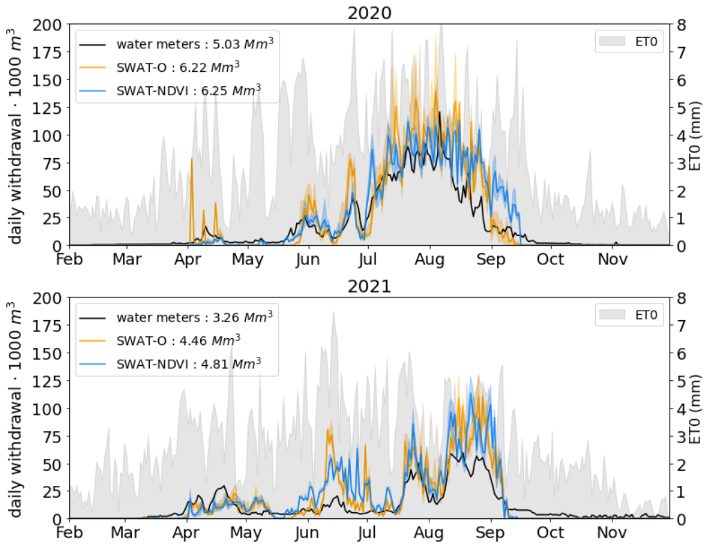
Figure 6 Simulated and measured daily irrigation withdrawals in the two managed rivers (Gimone and Marcaoué) for the years 2020 and 2021.

It can be seen that the timing and amounts of withdrawals are highly dependent on the year. The weather might therefore be the first determining factor for irrigation. The rainfall in June and July 2021 resulted in low evaporative demand and very low irrigation during this period. On the contrary, high temperatures and a lack of rain in July 2020 resulted in a high evaporative demand, followed by large amounts of irrigation.

Some differences can also be seen between simulated withdrawals in the SWAT-O and SWAT-NDVI modes. In particular, the peak of water demand in the SWAT-NDVI mode at the beginning of the irrigation season (June) is reduced in terms of intensity and spread in time compared to the SWAT-O mode. This is a direct effect of the spreading of emergence dates, which triggers a spread in crop management dates.

At the end of the 2020 irrigation season (September), the SWAT-NDVI mode produced a higher irrigation amount than the SWAT-O mode. This is due to a difference in crop phenology between the two setups: the NDVI showed that corn and soybean were not yet harvested and that their water needs were still high due to the high ET₀. On the contrary, in the SWAT-O mode, most crops were already harvested.

The remaining gaps between the simulations and measurements could be explained by several factors:

1. The actual irrigated fields are not known. Our choice to irrigate all corn, soybeans, vegetables and orchards in fields with slopes less than 10 % is consistent but arbitrary. As several authors (Demarez et al., 2019; Pageot et al., 2020; Puy et al., 2022) highlight, irrigated areas are the main driver of water withdrawals. Indeed, a 10 % error in areas logically leads to a 10 % error in withdrawals.

2. This graph compares the withdrawals that occur only in the two main rivers. We assumed that it represents 56 % of the total withdrawals, but the actual distribution of withdrawal origin might be slightly different.

3. Intrinsic uncertainty in the networked meters is very low, but errors could originate from the fact that only 60 % to 75 % of the intake points are equipped and that we extrapolated these withdrawal data to the missing intake points.

4. Water restrictions are frequent at the end of the low-water season but are not taken into account in the model. The overestimation in September 2020 can indeed be explained by the drought decree on 29 August 2020, which resulted in a 50 % reduction in withdrawals in the main rivers and the prohibition of irrigation from small tributaries. In contrast, 2021 was a wet year, and main rivers were been subjected to any restriction.

5. With April to June being a rainy period, Sentinel-2 images are often corrupted by clouds. During this period, summer crops are sown and begin to grow. For this reason, the linear interpolation between cloud-free images fails to reproduce the convex shape of the NDVI and leads to an overestimation, which results in an overestimation of the ET. Therefore, irrigation can also be overestimated during this period.

3.5 Effects of irrigation withdrawals on the river flow

In addition to the SWAT-O and SWAT-NDVI setups, a third setup was run: SWAT-O with no irrigation. Each setup was run four times with different sets of parameters (see Calibration section). In the following, the error bars or uncertainty margins refer to the range of values obtain with those four runs.

For further quantitative analysis, we distinguish between two periods: on the one hand, the high-flow period from November to May, over which period the calibration of hydrological processes has been performed, and on the other hand, the administrative low-flow period from June to October, where the flow is highly influenced by dam releases and irrigation withdrawals.

During the high-flow season, most of the metrics are not influenced by the introduction of the NDVI method into the model (Table 7-Up). The P_bias values rise from 5.7 % to 11.2 %, which is in the range of acceptable values (Moriasi et al., 2007). Since hydrological processes were calibrated without NDVI, a slight decrease in model performance could be expected after adding it.

Table 7 Scores for the SWAT-O and SWAT-NDVI setups for the years 2017 to 2021. At the top is the high-flow period from November to May. At the bottom is the low-flow period from June to October.

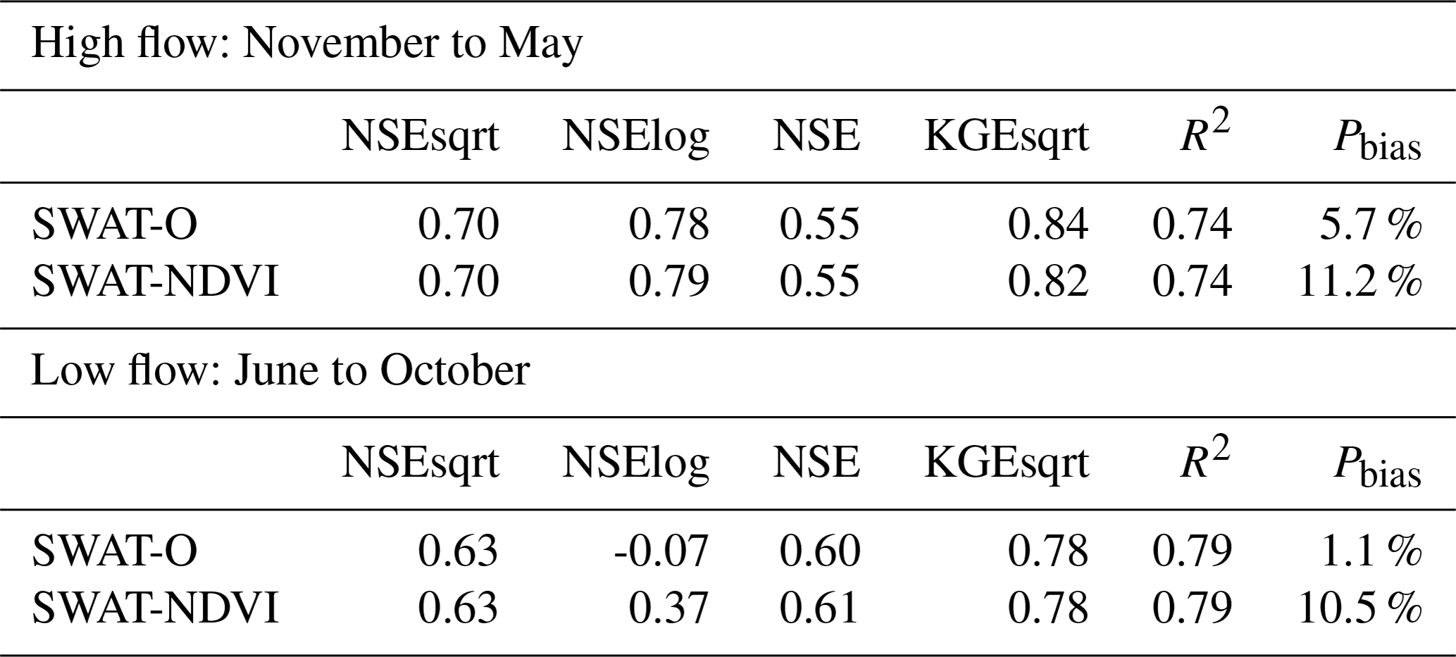
On the other hand, Table 7 (bottom) shows the metrics calculated over the low-flow season. The scores over this period barely changed, but the significant increase of NSElog from about 0 to close to 0.4 suggests an improvement in the low-flow simulation using the SWAT-NDVI mode.

Figure 7 shows the simulated streamflow at the outlet for the period where Sentinel-2 data are available (2017 to 2021). The graph focuses on the irrigation period, from April to October, where the differences between setups are more likely to be seen, and this is the period of interest regarding the water demand and the strategies for water management.

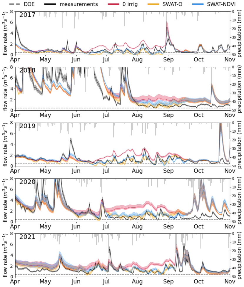
Figure 7 Simulation against measured daily outlet streamflow during the June–October period for 5 consecutive years. The SWAT-O and SWAT-NDVI setups are compared with the theoretical simulation without irrigation withdrawals.

The graph reflects as far as possible the uncertainties we are aware of. For simulation plots, plain lines are the median value, and the errors bars are minimum and maximum values obtained from the four runs with different parameters sets. In addition, there might be a ±10 % error in the measured flow rate values according to the water manager . This uncertainty is included in the graph using a colored range.

The minimal flow rate that has to be maintained (DOE) is also included as a horizontal line.

Significant differences can be observed between the three setups. On the one hand, both models fail to simulate the flow rate at the end of the low-flow seasons for 2018, 2019 and 2020, for which heavy rains occurred in October. The reason for this might be that a lot of small reservoirs – not taken into consideration in this study – are close to being empty at the end of summer and are filled up by the first heavy-rain period (bar plots in Fig. 7), leading to less flow reaching the river.

On the other hand, the comparison with the no-irrigation mode clearly shows the importance of taking into account agricultural practices (through withdrawals here) that account for more than half of the streamflow during summer in such a watershed. It shows that the order of magnitude of simulated withdrawals is correct, which is a second validation of the retrieved withdrawals.

Finally, the improved timing of withdrawals in the SWAT-NDVI setup has some visible effects on the streamflow, mostly at the beginning of irrigation season (June, July). The flow is smoother in this mode because it is subject to fewer peaks in withdrawals. In general, the SWAT-NDVI mode produces a higher discharge than the SWAT-O mode. This is due to the lower ET in the SWAT-NDVI mode compared to in the SWAT-O mode (Fig. 5) in addition to the lower amount of withdrawals (Fig. 6).

4 Conclusions and outlooks

This study deals with the modeling of crop phenology and irrigation withdrawals in an agricultural zone and their impact on downstream flows. The SWAT+ agro-hydrological model was chosen because it allows a spatialized and detailed description of crop management. Two modeling approaches were compared for crop management. The first modeling approach (SWAT-O) uses heat units to compute the emergence and senescence dates of crops, their growth rate and LAI, and then their ET. The second approach (SWAT-NDVI) uses Sentinel-2 remote sensing data, through the NDVI vegetation index, to determine all these features.

Before tackling the crop modeling, the calibration of hydrological fluxes was addressed. Because of the very influenced streamflow during summer, calibration was performed during the remaining months, from November to May. This uncommon calibration method relies on the assumption that parameters are independent of the time of the year, and this hypothesis has proven to be plausible in the course of this study. A strength of this study is admitting to the uncertainties due to calibration, taking this it into account in the analysis.

Then, focusing on crops, the SWAT-NDVI setup first allows us to better account for the spatial and temporal variability of the cultivated crops by spreading the emergence over time and over the watershed, which is more realistic. The modeled ET in this new setup follows the observed crop dynamics at the plot scale, even though the differences in ET seem to be barely significant at the watershed scale. The simulated daily withdrawals have been compared against daily irrigation data provided by the water manager. Both setups reproduce quite well the overall evolution of withdrawals throughout the year. However, the SWAT-NDVI mode shows the best performances at the beginning of the irrigation season without further calibration. This improvement can mainly be attributed to the spreading of crop management dates.

In our watershed, irrigation withdrawals and dam releases are the main determining factors for the river flow in summer. Since dam releases are known and irrigation withdrawals are simulated, the model is able to provide satisfactory daily streamflows in low-flow periods. The results suggest that the SWAT-NDVI mode allows for slightly better accuracy for very low flows, but this would need to be confirmed by other experiments.

To conclude, this study shows that it is possible to simulate a very influenced streamflow with modeling tools. Indeed, very few modelers could focus on daily flow during low-flow periods due to the difficulties in modeling both hydrology and anthropogenic processes. In this study, we assessed two methods for crop dynamics that allow us to retrieve withdrawals and flow dynamics during irrigation periods with an unusual accuracy.

It would of course be interesting to reproduce this experiment in different watersheds with different climate and agricultural practices. In areas where land use, crop dynamics and irrigated areas are not well known, remote sensing methods could be of great help. In this study, the hypothesis about irrigated areas appeared to be sufficient. However, in other watersheds where fewer plots are irrigated, maps of irrigated areas could be necessary (Pageot et al., 2020). In addition, in order to obtain more accurate emergence dates, radar images that are not affected by clouds could be used in combination with optical images (Rolle et al., 2022).

In most watersheds, the lack of knowledge about the origin of withdrawals still remains a limitation of our approach. Finally, a major unknown of many watersheds is the small reservoirs that may have a huge impact on the flow rate but about which very little information is available (Boisson et al., 2022).