On the need for physical constraints in deep learning rainfall–runoff projections under climate change: a sensitivity analysis to warming and shifts in potential evapotranspiration

Deep learning (DL) rainfall–runoff models outperform conceptual, process-based models in a range of applications. However, it remains unclear whether DL models can produce physically plausible projections of streamflow under climate change. We investigate this question through a sensitivity analysis of modeled responses to increases in temperature and potential evapotranspiration (PET), with other meteorological variables left unchanged. Previous research has shown that temperature-based PET methods overestimate evaporative water loss under warming compared with energy budget-based PET methods. We therefore assume that reliable streamflow responses to warming should exhibit less evaporative water loss when forced with smaller, energy-budget-based PET compared with temperature-based PET. We conduct this assessment using three conceptual, process-based rainfall–runoff models and three DL models, trained and tested across 212 watersheds in the Great Lakes basin. The DL models include a Long Short-Term Memory network (LSTM), a mass-conserving LSTM (MC-LSTM), and a novel variant of the MC-LSTM that also respects the relationship between PET and evaporative water loss (MC-LSTM-PET). After validating models against historical streamflow and actual evapotranspiration, we force all models with scenarios of warming, historical precipitation, and both temperature-based (Hamon) and energy-budget-based (Priestley–Taylor) PET, and compare their responses in long-term mean daily flow, low flows, high flows, and seasonal streamflow timing. We also explore similar responses using a national LSTM fit to 531 watersheds across the United States to assess how the inclusion of a larger and more diverse set of basins influences signals of hydrological response under warming. The main results of this study are as follows:

1. The three Great Lakes DL models substantially outperform all process-based models in streamflow estimation. The MC-LSTM-PET also matches the best process-based models and outperforms the MC-LSTM in estimating actual evapotranspiration.

2. All process-based models show a downward shift in long-term mean daily flows under warming, but median shifts are considerably larger under temperature-based PET (−17 % to −25 %) than energy-budget-based PET (−6 % to −9 %). The MC-LSTM-PET model exhibits similar differences in water loss across the different PET forcings. Conversely, the LSTM exhibits unrealistically large water losses under warming using Priestley–Taylor PET (−20 %), while the MC-LSTM is relatively insensitive to the PET method.

3. DL models exhibit smaller changes in high flows and seasonal timing of flows as compared with the process-based models, while DL estimates of low flows are within the range estimated by the process-based models.

4. Like the Great Lakes LSTM, the national LSTM also shows unrealistically large water losses under warming (−25 %), but it is more stable when many inputs are changed under warming and better aligns with process-based model responses for seasonal timing of flows.

Ultimately, the results of this sensitivity analysis suggest that physical considerations regarding model architecture and input variables may be necessary to promote the physical realism of deep-learning-based hydrological projections under climate change.

1 Introduction

Rainfall–runoff models are used throughout hydrology in a range of applications, including retrospective streamflow estimation (Hansen et al., 2019), streamflow forecasting (Demargne et al., 2014), and prediction in ungauged basins (Hrachowitz et al., 2013). Work over the past few years has demonstrated that deep learning (DL) rainfall–runoff models (e.g., Long Short-Term Memory networks (LSTMs); Hochreiter and Schmidhuber, 1997) outperform conventional process-based models in each of these applications, especially when those DL models are trained with large datasets collected across watersheds with diverse climates and landscapes (Kratzert et al., 2019a, b; Feng et al., 2020; Ma et al., 2021; Gauch et al., 2021a, b; Nearing et al., 2021). For example, in one extensive benchmarking study, Mai et al. (2022a) found that a regionally trained LSTM outperformed 12 other lumped and distributed process-based models of varying complexity in rivers and streams throughout the Great Lakes basin. These and similar results have led some to argue that DL models represent the most accurate and spatially extrapolatable rainfall–runoff models available (Nearing et al., 2022).

However, there remains one use case of rainfall–runoff models where the superiority of DL is unclear: long-term projections of streamflow under climate change. Past studies using DL rainfall–runoff models for hydrological projections under climate change are rare (Lee et al., 2020; Li et al., 2022), and few have evaluated their physical plausibility (Razavi, 2021; Reichert et al., 2023; Zhong et al., 2023). A reasonable concern is whether DL rainfall–runoff models can extrapolate hydrological response under unprecedented climate conditions, given that they are entirely data driven and do not explicitly represent the physics of the system. It is not clear a priori whether this concern has merit, because DL models fit to a large and diverse set of basins have the benefit of learning hydrological response across climate and landscape gradients. In so doing, the model can, for example, learn hydrological responses to climate in warmer regions and then transfer this knowledge to projections of streamflow in cooler regions subject to climate change induced warming. In addition, past work has shown that LSTMs trained only to predict streamflow have memory cells that strongly correlate with independent measures of soil moisture and snowpack (Lees et al., 2022), suggesting that DL hydrological models can learn fundamental hydrological processes. A potential implication of this finding might be that these models can produce physically plausible streamflow predictions under new climate conditions.

It is challenging to assess the physical plausibility of DL-based hydrological projections under substantially different climate conditions, because there are no future observations against which to compare. This challenge is exacerbated by significant uncertainty in process-based model projections under alternative climates, which makes establishing reliable benchmarks difficult. Future process-based model projections can vary widely due to both parametric and structural uncertainty (Bastola et al., 2011; Clark et al., 2016; Melsen et al., 2018), and even for models that exhibit similar performance under historical conditions (Krysanova et al., 2018). Assumptions around stationary model parameters are not always valid (Merz et al., 2011; Wallner and Haberlandt, 2015), and added complexity for improved process representation is not always well supported by data (Clark et al., 2017; Towler et al., 2023; Yan et al., 2023). Together, these challenges highlight the difficulty in establishing good benchmarks of hydrological response under alternative climates against which to compare and evaluate DL-based hydrological projections under climate change.

Recently, Wi and Steinschneider (2022) (hereafter WS22) forwarded an experimental design to evaluate the physical plausibility of DL hydrological responses to new climates, in which DL hydrological models were forced with historical precipitation and temperature, but with temperatures adjusted by up to 4 ^∘C. Based on past literature, WS22 posited that in non-glaciated regions, physically plausible hydrological responses should show an increase in water loss, defined as water that enters the watershed via precipitation but never contributes to streamflow because it is “lost” to a terminal sink. Specifically, WS22 assumed that evaporative water loss should increase and annual average streamflow should decline compared with a baseline simulation due to increases in potential evapotranspiration (PET) with warming (and no changes in precipitation). Results showed that an LSTM trained to 15 watersheds in California often led to misleading increases in annual runoff under warming, while this phenomenon was less likely (though still present) in a DL model trained to 531 catchments across the United States. WS22 also conducted their experiment with physics-informed machine learning (PIML) models (Karpatne et al., 2017; Karniadakis et al., 2021), using process-based model output directly as input to the LSTM (similar to Konapala et al., 2020; Lu et al., 2021; Frame et al., 2021a) or as additional target variables in a multi-output architecture. The former approach had some success in removing instances of increasing runoff ratio with warming, although this was dependent on the process-based model used.

Other PIML approaches that more directly adjust the architecture of DL rainfall–runoff models may be better suited for improving long-term streamflow projections under climate change without requiring an accurate process-based model. For instance, Hoedt et al. (2021) introduced a mass conserving LSTM (MC-LSTM) that ensures cumulative streamflow predictions do not exceed precipitation inputs. Hybrid models present a related approach, where DL modules are combined with process-based model structures (Jiang et al., 2020; Feng et al., 2022, 2023a; Hoge et al., 2022). In some cases, these architectural changes can degrade performance compared with a standard LSTM (Frame et al., 2022b, 2002a; Feng et al., 2023b), but other times such changes can be beneficial (Feng et al., 2023a). To date, the benefits of mass conserving architectures have not been tested when employed under previously unobserved climate change.

For all models considered in WS22, a major focus was evaluating the direction of annual total runoff change in the presence of warming and no change in precipitation. However, that study did not consider the magnitude of runoff change and how it relates to projected changes in PET. As we argue below, this comparison provides a unique way to assess the physical plausibility of future hydrological projections. Several studies have investigated the effects of different PET estimation methods on the magnitude of PET and runoff change in a warming climate (Lofgren et al., 2011; Shaw and Riha, 2011; Lofgren and Rouhana, 2016; Milly and Dunne, 2017; Lemaitre-Basset et al., 2022). Broadly, these studies have shown that temperature-based PET estimation methods (e.g., Hamon, Thornthwaite) substantially overestimate increases in PET under warming as compared with energy-budget-based PET estimation methods (e.g., Penman–Monteith, Priestley–Taylor) and consequently lead to unrealistic declines in streamflow under climate change. This is because the actual drying power of the atmosphere is driven by the availability of energy at the surface from net radiation, the current moisture content of the air, temperature (and its effect on the water holding capacity of the air and vapor pressure deficit), and wind speeds. Energy-budget-based methods, while imperfect and at times empirical (Greve et al., 2019; Liu et al., 2022), account for some or all of these factors in ways that are generally consistent with their causal impact on PET, while temperature-based methods estimate PET using strictly empirical relationships based largely or entirely on temperature. The latter approach works sufficiently well for rainfall–runoff modeling under historical conditions because of the strong correlation between temperature, net radiation, and PET on seasonal timescales, even though this correlation weakens considerably at shorter timescales (Lofgren et al., 2011). Under climate change, consistent and prominent increases are projected for temperature, but projected changes are less prominent or more uncertain for other factors affecting PET (Lin et al., 2018; Pryor et al., 2020, Liu et al., 2020). Consequently, temperature-based PET methods substantially overestimate future projections of PET compared with energy-budget-based methods (Lofgren et al., 2011; Shaw and Riha, 2011; Lofgren and Rouhana, 2016; Milly and Dunne, 2017; Lemaitre-Basset et al., 2022).

As argued by Lofgren and Rouhana (2016), the bias in PET and runoff that results from different PET estimation methods under warming provides a unique opportunity to assess the physical plausibility of hydrological projections under climate change. In this study, we adopt this strategy for DL rainfall–runoff models through a sensitivity analysis in which both conceptual, process-based and DL hydrological models are trained with either temperature-based or energy-budget-based estimates of PET, along with other meteorological data (precipitation, temperature). These models are then forced with the historical precipitation and temperature series but with the temperatures warmed by an additive factor and PET calculated from the warmed temperatures using both PET estimation methods. We show that the process-based models (1) exhibit similar performance in historical training and testing periods when using either temperature-based or energy-budget-based PET estimates but (2) exhibit substantially larger long-term mean streamflow declines under warming when using future PET estimated with a temperature-based method. If the DL rainfall–runoff models follow the same pattern, this would suggest that these models are able to learn the role of PET on evaporative water loss. However, if DL-based models estimate similarly large long-term mean streamflow declines regardless of the method used to estimate and project PET, this would suggest that the DL models did not learn a mapping between PET and evaporative water loss. Rather, the DL models learned the historical (but non-causal) correlation between temperature and evaporative water loss, and then incorrectly extrapolated that effect into the future with warmer temperatures. We show this latter outcome to be the case, which indicates that we either need to build models on large data sets that comprise similar conditions to the ones under climate change, or we need to guide the model selection using theory (e.g., see Karpatne et al., 2017).

We conduct the experiment above in a case study on 212 watersheds across the Great Lakes basin, using both standard and PIML-based LSTMs. We show that a standard LSTM produces unrealistic hydrological responses to warming because it relies on historical and geographically pervasive correlations between temperature and PET to estimate streamflow losses. We also show that PIML-based DL models are better able to relate changes in temperature and PET to streamflow change, especially those PIML approaches that directly map PET to evaporative water loss in their architecture.

The Great Lakes provide an important case study for this work, given their importance to the culture, ecosystems, and economy of North America (Campbell et al., 2015; Steinman et al., 2017). Projections of future water supplies and water levels in the Great Lakes are highly uncertain (Gronewold and Rood, 2019), in part because of uncertainty in future runoff draining into the lakes from a large contributing area (Kayastha et al., 2022), much of which is ungauged (Fry et al., 2013). Improved rainfall–runoff models that can regionalize across the entire Great Lakes basin are necessary to help address this challenge, and therefore an auxiliary goal of this work is to contribute PIML rainfall–runoff models to the Great Lakes Runoff Intercomparison Project Phase 4 presented in Mai et al. (2022a). This study currently provides one of the most robust benchmarks comparing DL rainfall–runoff models to a range of process-based models, and therefore we design our experiment to be consistent with the data and model development rules outlined in that intercomparison project.

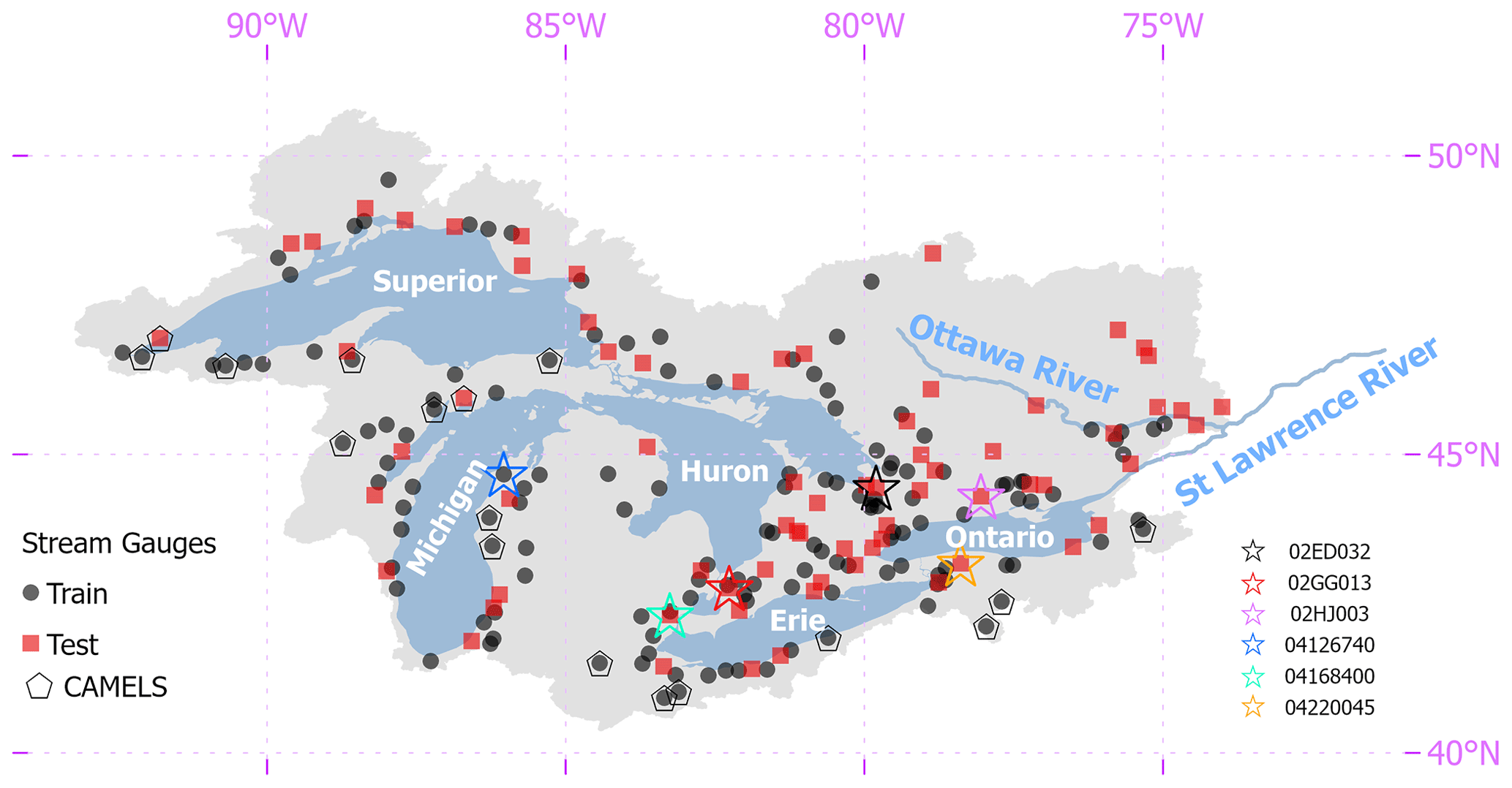
Figure 1 Great Lakes domain with training and testing streamflow gauges used throughout this study. A subset of 17 of these gauges that are also in the CAMELS database are highlighted, as are six sites used to present select results in Sect. 4.

2 Data

This study focuses on 212 watersheds draining into the Great Lakes and Ottawa River, which are all located in the St. Lawrence River basin (Fig. 1). For direct comparability to previous results from the Great Lakes Runoff Intercomparison Project, all data for these watersheds are taken directly from the work in Mai et al. (2022a) and include daily streamflow time series, meteorological forcings, geophysical attributes for each watershed, and auxiliary hydrological fluxes. Daily streamflow were gathered from the U.S. Geological Survey and Water Survey Canada between January 2000 and December 2017. All streamflow gauging stations have a drainage area greater than or equal to 200 km² and less than 5 % missing data in the study period. The watersheds are evenly distributed across the five lake basins and the Ottawa River basin, and they represent a range of land use and land cover types and degrees of hydrological alteration from human activity. In the experiments described further below, 141 of the watersheds are designated as training sites and the remaining 71 watersheds are used for testing (see Fig. 1). In addition, the period between January 2000 to December 2010 is reserved for model training (termed the training period) and the period between January 2011–December 2017 is used for model testing (termed the testing period).

Meteorological forcings are taken from the Regional Deterministic Reanalysis System v2, which is an hourly, 10 km dataset available across North America (Gasset et al., 2021). Hourly precipitation, net incoming shortwave radiation (R_s), and temperature are aggregated into a basin-wide daily precipitation average, daily R_s average, and daily minimum and maximum temperature. We note that the precipitation data from the Regional Deterministic Reanalysis System v2 are produced from the Canadian Precipitation Analysis, which combines available surface observations of precipitation with a short-term reforecast provided by the 10 km Regional Deterministic Reforecast System, that is, the precipitation data are not model based but rather is based on gauged data and spatially interpolated using information from modeled output.

Table 1 Watershed attributes used in the deep learning models developed in this work (adapted from Mai et al., 2022a).

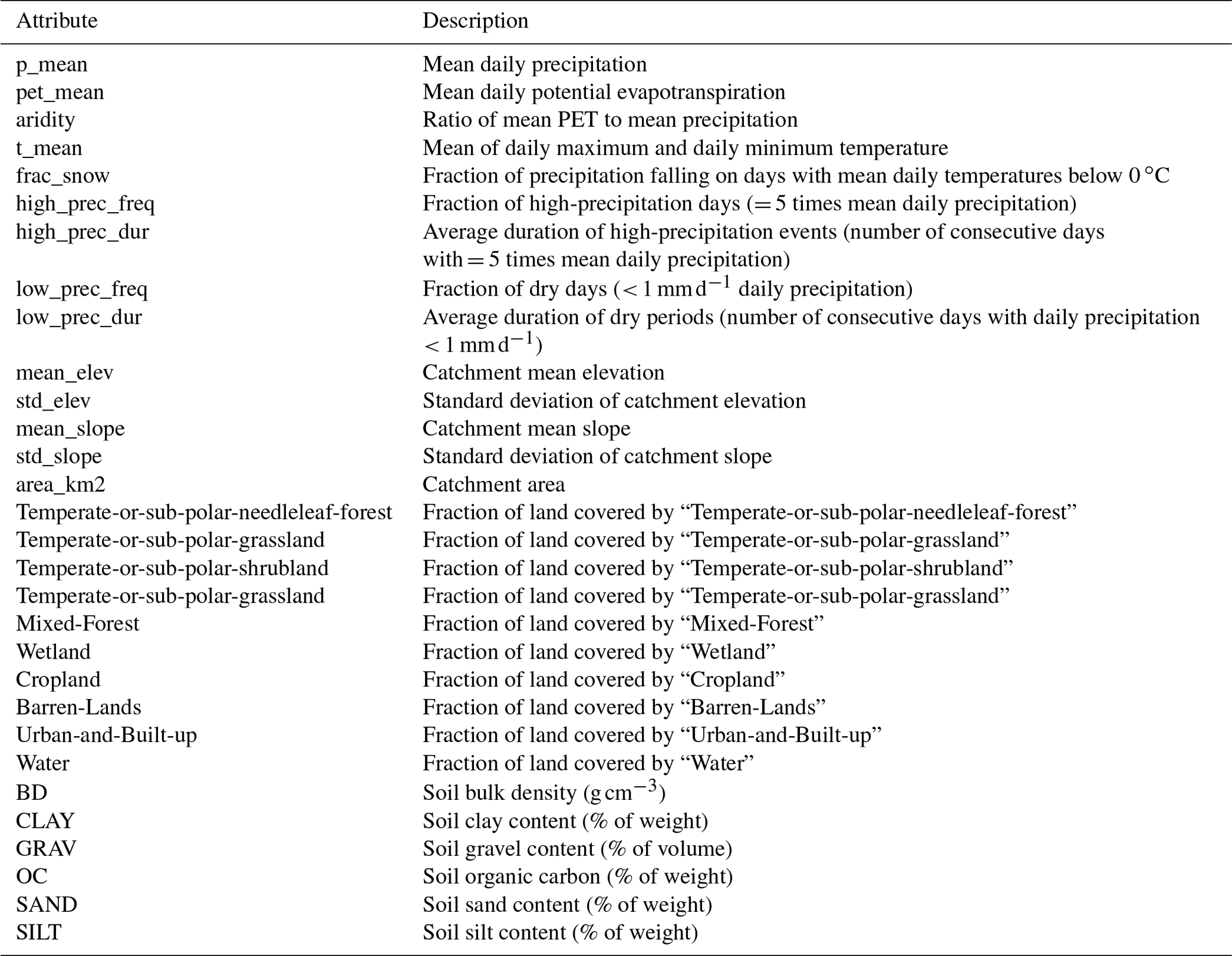
Geophysical attributes for each watershed were collected from a variety of sources. Basin-average statistics of elevation and slope were derived from the HydroSHEDS dataset (Lehner et al., 2008), which provides a digital elevation model with 3 arcsec resolution. Soil properties (e.g., soil texture and classes) were gathered from the Global Soil Dataset for Earth System Models (Shangguan et al., 2014), which is available at a 30 arcsec resolution. Land cover data at a 30 m resolution and based on Landsat imagery from 2010–2011 were derived from the North American Land Change Monitoring System (NALCMS, 2017). These geophysical datasets were used to derive basin-averaged attributes for each watershed listed in Table 1.

Finally, we also collect daily actual evapotranspiration (AET) for each watershed in millimeters per day, which was originally taken from the Global Land Evaporation Amsterdam Model (GLEAM) v3.5b dataset (Martens et al., 2017). GLEAM couples remotely sensed observations of microwave vegetation optical depth, a multi-layer soil moisture model driven by observed precipitation and assimilating satellite surface soil moisture observations, and Priestly–Taylor-based estimates of PET to derive an estimate of AET for each day. The daily data were originally available over the entire study domain at a 0.25^∘ resolution between 2003 and 2017, and were aggregated to basin-wide totals for each watershed. While AET from GLEAM is still uncertain, it provides a useful, independent, remote-sensing-based benchmark against which to compare rainfall–runoff model estimates of AET.

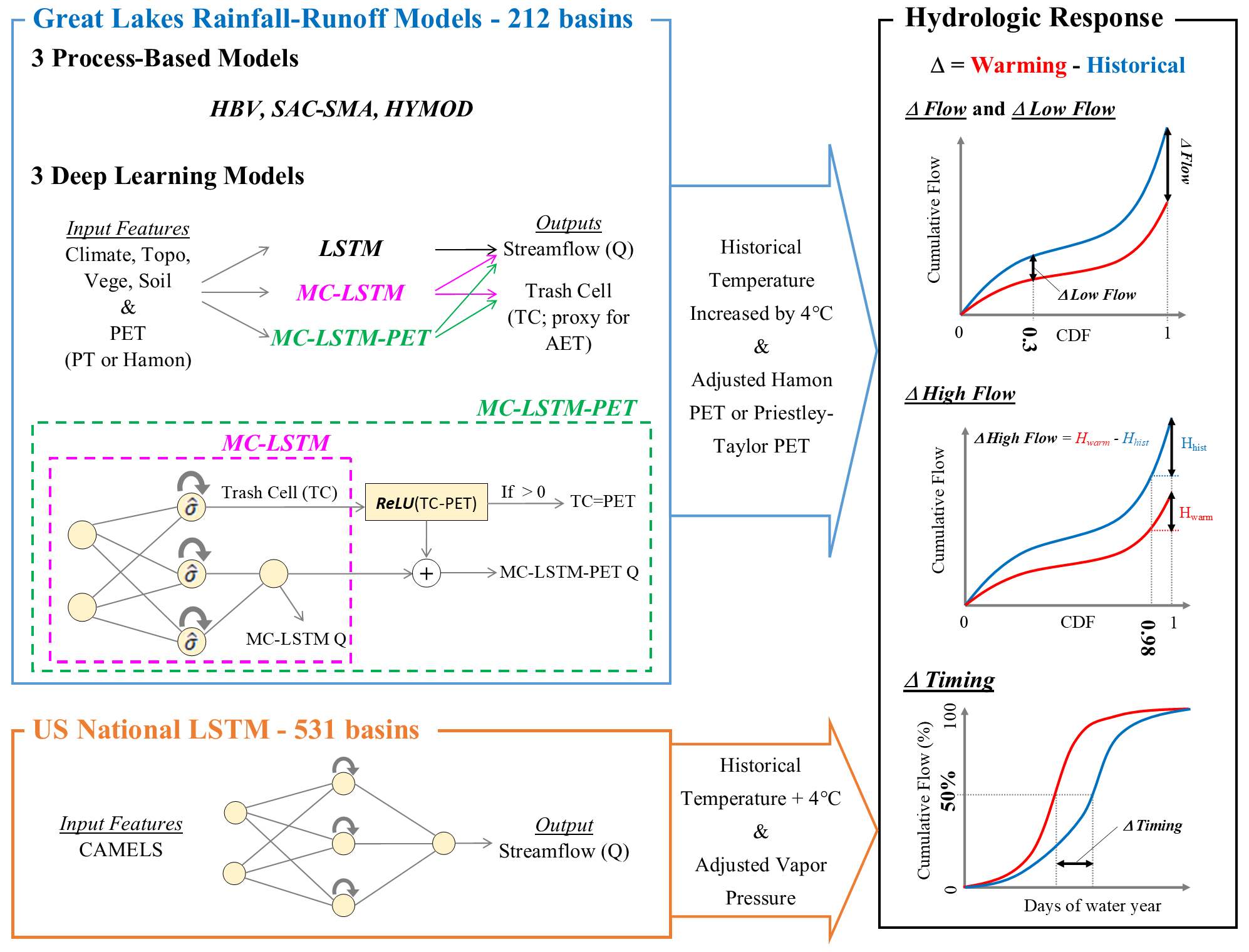
Figure 2 Overview of experiment design. Three deep learning rainfall–runoff models (LSTM, MC-LSTM, and MC-LSTM-PET) and three conceptual, process-based models (HBV, SAC-SMA, and HYMOD) are trained and tested across 212 watersheds throughout the Great Lakes basin. Models are validated by comparing predictions to streamflow (Q) and actual evapotranspiration (AET). All models are then forced with historical meteorology, but with historical temperatures warmed by 4 ^∘C and potential evapotranspiration (PET) updated based on those warmed temperatures using either the Hamon or Priestley–Taylor method. Hydrological model responses across all models are then compared in terms of long-term mean daily flows, low flows, high flows, and streamflow seasonal timing statistics. The experiment is also repeated with an LSTM fit to 531 basins across the contiguous United States, except that model uses a different set of inputs, does not use PET as an input, and vapor pressure is also adjusted along with temperature.

3 Methods

We design an experiment to test the two primary hypotheses of this study, namely that a standard LSTM will overestimate evaporative water losses under warming because of an overreliance on historical correlations between temperature and PET, while this effect will be lower in PIML-based rainfall–runoff models designed to better account for evaporative water loss in the system. To conduct this experiment, we develop three different DL rainfall–runoff models to predict daily streamflow across the Great Lakes region, as well as three conceptual, process-based models as benchmarks, each of which is trained twice with either an energy-budget-based or temperature-based estimate of PET. The DL models include a regional LSTM very similar to the model in Mai et al. (2022a), an MC-LSTM that conserves mass, and a new variant of the MC-LSTM that also respects the relationship between PET and evaporative water loss (termed MC-LSTM-PET). After comparing historical model performance, we conduct a sensitivity analysis on all models in which historical temperatures are warmed by 4 ^∘C, PET is updated based on those warmed temperatures, and all other meteorological variable time series are left unchanged from historical values. This is a similar approach to that taken in WS22, but in contrast to that study, this work (1) focuses on the magnitude of streamflow response to warming under two different PET formulations, (2) considers a different set of physics-informed DL models in which the architecture (rather than the inputs or targets) of the model are changed to better preserve physical plausibility under shifts in climate, and (3) evaluates an expanded set of hydrological metrics to better understand both the plausibility and the variability of responses across the different models. Finally, in a subset of the analysis, we also utilize a fourth DL model, the LSTM used in WS22 that was previously fit to 531 basins across the CONUS (Kratzert et al., 2021), which uses daily precipitation, maximum and minimum temperature, radiation, and vapor pressure as input but not PET. This model is used to evaluate whether a DL model fit to many more watersheds that span a more diverse gradient of climate conditions behaves differently under warming than an LSTM fit only to locations in the Great Lakes basin. Figure 2 presents an overview of our experimental design.

3.1 Models

3.1.1 Benchmark conceptual models

We calibrate three conceptual, process-based hydrological models as benchmarks, including the Hydrologiska Byråns Vattenbalansavdelning (HBV) model (Bergström and Forsman, 1973), HYMOD (Boyle, 2001), and the Sacramento Soil Moisture Accounting (SAC-SMA) model (Burnash, 1995) coupled with SNOW-17 (Anderson, 1976). These models are developed as lumped, conceptual models for each watershed and were selected for several reasons. First, in the Great Lakes Intercomparison Project (Mai et al., 2022a), HYMOD was one of the best performing process-based models for both streamflow and AET estimation. SAC-SMA is widely used in the United States, forming the core hydrological model in NOAA's Hydrologic Ensemble Forecasting System (Demargne et al., 2014). This model was also shown to outperform the National Water Model across hundreds of catchments in the United States (Nearing et al., 2021). We also found in WS22 that AET from SAC-SMA matched the seasonal pattern of MODIS-derived AET well across California. HBV is also used for operational forecasting in multiple countries (Olsson and Lindstrom, 2008; Krøgli et al., 2018) and performs very well in hydrological model intercomparison projects (Breuer et al., 2009; Plesca et al., 2012; Beck et al., 2016, 2017; Seibert and Bergström, 2022). Importantly, the HYMOD, SAC-SMA, and HBV models can exhibit significant intermodel differences in behavior, dominant processes, and performance controls through time, even in situations where they share similar process formulations (Herman et al., 2013).

We calibrate the process-based models with the genetic algorithm from Wang (1991) to minimize the mean-squared error (MSE), using a population size equal to 100 times the number of parameters, evolved over 100 generations, and with a spin-up period of 1 year. Each benchmark model is calibrated separately to each of the 141 training sites using the temporal train/test split described in Sect. 2, and training is repeated 10 separate times with different random initializations to account for uncertainty in the training process and to estimate parametric uncertainty. Benchmark models are calibrated for the 71 testing sites in two ways: (1) separate models are trained for the testing sites during the training period; and (2) each testing site is assigned a donor from among the 141 training sites, and the calibrated parameters from that donor site are transferred to the testing site. The first of these approaches enables a comparison between DL models fit only to the training sites to benchmark models developed for the testing sites, i.e., a spatial out-of-sample versus in-sample comparison. The second of these approaches enables a more direct spatial out-of-sample comparison between DL and benchmark models. We note that donor sites were used to assign model parameters to testing sites in the benchmarking study of Mai et al. (2022a), and to retain direct comparability to the results of that work we use the same donor sites for each testing site. Donor sites were selected based on spatial proximity while also prioritizing donor sites that were nested within the watershed of the testing site.

3.1.2 LSTM

We develop a single, regional LSTM for predicting daily streamflow across the Great Lakes region. In the LSTM, nodes within hidden layers feature gates and cell states that address the vanishing gradient problem of classic recurrent neural networks and help capture long-term dependencies between input and output time series. The model defines a D-dimensional vector of recurrent cell states c[t] that is updated over a sequence of $t=\mathrm{1},\mathrm{\dots }s$, T time steps based on a sequence of inputs $x=\mathit{x}\left[\mathrm{1}\right],\mathrm{\dots },\mathit{x}\left[T\right]$, where each input x[t] is a K-dimensional vector of features. Information stored in the cell states is then used to update a D-dimensional vector of hidden states h[t], which form the output of the hidden layer in the model. The structure of the LSTM is given as follows:

$$\begin{array}{}\text{(1a)}& {\displaystyle }\mathit{i}\left[t\right]=\mathit{\sigma }{W}_i\mathit{x}\left[t\right]+U_i\mathit{h}[t-\mathrm{1}]+b_i)\text{(1b)}& {\displaystyle }\mathit{f}\left[t\right]=\mathit{\sigma }{W}_f\mathit{x}\left[t\right]+U_f\mathit{h}[t-\mathrm{1}]+b_f)\text{(1c)}& {\displaystyle }\mathit{g}\left[t\right]=\text{tanh }{W}_g\mathit{x}\left[t\right]+U_g\mathit{h}[t-\mathrm{1}]+b_g)\text{(1d)}& {\displaystyle }\mathit{o}\left[t\right]=\mathit{\sigma }{W}_o\mathit{x}\left[t\right]+U_o\mathit{h}[t-\mathrm{1}]+b_o)\text{(1e)}& {\displaystyle }\mathit{c}\left[t\right]=\mathit{f}\left[t\right]\odot \mathit{c}[t-\mathrm{1}]+\mathit{i}\left[t\right]\odot \mathit{g}\left[t\right]\text{(1f)}& {\displaystyle }\mathit{h}\left[t\right]=\mathit{o}\left[t\right]\odot \text{tanh }\mathit{c}\left[t\right])\text{(1g)}& {\displaystyle }\mathit{y}\left[T\right]=\mathrm{ReLU}\left(W_y\mathit{h}\right[T]+b_y).\end{array}$$

Here, the input gate (i[t]) controls how candidate information (g[t]) from inputs and previous hidden states flows to the current cell state (c[t]), the forget gate (f[t]) enables removal of information within the cell state over time, and the output gate (o[t]) controls information flow from the current cell state to the hidden layer output. All bolded terms are vectors and ⊙ denotes element-wise multiplication. To produce streamflow predictions, h[T] at the last time step in the sequence is passed through a fully connected layer to a single-node output layer (i.e., a many-to-one formulation). We ensure non-negative streamflow predictions using the rectified linear unit (ReLU) activation function for the output neuron, expressed as $\mathrm{ReLU}\left(x\right)=\text{max}(\mathrm{0},x)$. Importantly, there are no constraints requiring the mass of water entering as precipitation to be conserved within this architecture.

The LSTM takes K=39 input features: 9 dynamic and 30 static. The dynamic input features are basin-averaged climate, including daily precipitation, maximum temperature, minimum temperature, net incoming shortwave radiation, specific humidity, surface air pressure, zonal and meridional components of wind, and PET. The static features represent catchment attributes (see Table 1) and are repeated for all time steps in the input sequences x. All input features are standardized before training (by subtracting the mean and dividing by the standard deviation for data across all training sites in the training period). Note that we do not standardize the observed streamflow besides dividing by drainage area to represent streamflow in units of millimeters.

We train the LSTM by minimizing the mean-squared error averaged over the 141 training watersheds during the training period:

$$\begin{array}{}\text{(2)}& \mathrm{MSE}={\displaystyle \frac{\mathrm{1}}{N}}{\sum }_{n=\mathrm{1}}^N{\displaystyle \frac{\mathrm{1}}{T_n}}{\sum }_{t=\mathrm{1}}^{T_n}{\left({\widehat{Q}}_{n,t}-Q_{n,t}\right)}^{\mathrm{2}},\end{array}$$

where N is the number of training watersheds and T_n is the number samples in the nth watershed. ${\widehat{Q}}_{n,t}$ and Q_n,t are, respectively, the streamflow prediction and observation for basin n and day t. To estimate ${\widehat{Q}}_{n,t}$, we feed into the network an input sequence for the past T = 365 d. The model was developed with 1 hidden layer composed of D = 256 nodes, a mini-batch size of 256, a learning rate of 0.0005, and a drop-out rate of 0.4, and it was trained across 30 epochs. All hyperparameters (number of hidden layer nodes, mini-batch size, learning rate, dropout rate, and number of epochs) were selected in a 5-fold cross-validation on the training sites (see Table S2 in the Supplement for details on grid search). Network weights are tuned using the ADAM optimizer (Kingma and Ba, 2015). The model is trained 10 separate times with different random initializations to account for uncertainty in the training process.

For the evaluation of streamflow responses to warming, we also use an LSTM taken from Kratzert et al. (2021) and employed in WS22, which was fit to 531 basins across the contiguous United States (hereafter called the “national LSTM”). This model was trained using a different set of data compared with our Great Lakes LSTM but also used a mix of dynamic and static features, all of which were drawn from the Catchment Attributes and Meteorology for Large-Sample Studies (CAMELS) dataset (Newman et al., 2015). This model uses daily precipitation, maximum and minimum temperature, shortwave downward radiation, and vapor pressure as input but not PET. However, we note that temperature, radiation, and vapor pressure are the three major inputs (besides wind speeds) needed to calculate energy-budget-based PET. There are 29 CAMELS watersheds located within the Great Lakes basin, and 17 of those 29 watersheds were also used in the training and testing sets for the Great Lakes LSTM (see Fig. 1).

3.1.3 MC-LSTM

Following Hoedt et al. (2021) and Frame et al. (2021b), we adapt the architecture of the LSTM into a mass conserving MC-LSTM that preserves the water balance within the model, i.e., the total quantity of precipitation entering the model is tracked and redistributed to streamflow and losses from the watershed. Using similar notation as for the LSTM above, the model structure is given as follows:

$$\begin{array}{}\text{(3a)}& {\displaystyle }\mathit{i}\left[t\right]=\widehat{\mathit{\sigma }}\left(W_i\mathit{x}\right[t]+U_i\mathit{c}[t-\mathrm{1}]+V_{i}a[t]+b_i)\text{(3b)}& {\displaystyle }\mathit{o}\left[t\right]=\mathit{\sigma }\left(W_o\mathit{x}\right[t]+U_o\mathit{c}[t-\mathrm{1}]+V_{o}a[t]+b_o)\text{(3c)}& {\displaystyle }\mathbf{R}\left[t\right]=\widehat{\mathit{\sigma }}\left(W_R\mathit{x}\right[t]+U_R\mathit{c}[t-\mathrm{1}]+V_{R}a[t]+b_R)\text{(3d)}& {\displaystyle }\mathit{m}\left[t\right]=\mathbf{R}\left[t\right]\mathit{c}[t-\mathrm{1}]+\mathit{i}\left[t\right]\mathit{x}\left[t\right]\text{(3e)}& {\displaystyle }\mathit{c}\left[t\right]=(\mathrm{1}-\mathit{o}[t\left]\right)\odot \mathit{m}\left[t\right]\text{(3f)}& {\displaystyle }\mathit{h}\left[t\right]=\mathit{o}\left[t\right]\odot \mathit{m}\left[t\right].\end{array}$$

Here, the inputs to the model are split between quantities x[t] to be conserved (i.e., precipitation), and non-conservative inputs a[t] (i.e., temperature, wind speeds, PET, catchment properties, etc.). Water in the system is stored in the D-dimensional vector m[t] and is updated at each time step based on water left over from the previous time step (c[t−1]) and water entering the system at the current time step (x[t]). The input gate i[t] and a redistribution matrix R[t] are designed to ensure water is conserved from c[t−1] and x[t] to m[t], by basing these quantities on a normalized sigmoid activation function:

$$\begin{array}{}\text{(4)}& \widehat{\mathit{\sigma }}\left(z_j\right)={\displaystyle \frac{\mathit{\sigma }\left(z_j\right)}{{\sum }_j\mathit{\sigma }\left(z_j\right)}}.\end{array}$$

Here, σ(⋅) is the sigmoid activation function, while $\widehat{\mathit{\sigma }}(\cdot )$ is a normalized sigmoid activation that produces a vector of fractions that sum to unity. The normalized sigmoid activation function is applied column-wise to the matrix R[t].

The mass in m[t], which is stored across D elements in the vector, is then distributed to the output of the hidden layer, h[t], or the next cell state, c[t]. To account for water losses from evapotranspiration or other sinks, one element of the D-dimensional vector h[t] is considered a “trash cell” and the output of this cell is ignored when calculating the final streamflow prediction, which at time T is given by the sum of outgoing water mass:

$$\begin{array}{}\text{(5)}& y\left[T\right]={\sum }_{d=\mathrm{1}}^{D-\mathrm{1}}{h}_d\left[T\right].\end{array}$$

Here, the Dth cell of h (h_D)T is set as the trash cell, and water allocated to this cell at each time step $t=\mathrm{1},\mathrm{\dots },T$ is lost from the system. We note that the MC-LSTM was trained in the same way as the LSTM (i.e., same inputs, loss function, training and test sets, hyperparameter selection process, and number of ensemble members with random initialization).

3.1.4 MC-LSTM-PET

We also propose a novel variant of the MC-LSTM that requires water lost from the system to not exceed PET (hereafter referred to as the MC-LSTM-PET). In the original MC-LSTM, any amount of water can be delegated to the trash cell h_D. Therefore, while water is conserved in the MC-LSTM, the model has the freedom to transfer any amount of water from m[t] to the trash cell (and out of the hydrological system) as it seeks to improve the loss function during training. This has the benefit of handling biased data, e.g., cases where the precipitation input to the system is systematically too high compared with the measured outflow. However, this structure also has the drawback of potentially removing more water from the system than is physically plausible. To address this issue, we propose a small change to the architecture of the MC-LSTM, where any water relegated to the trash cell that exceeds PET at time t is directed back to the stream:

$$\begin{array}{}\text{(6)}& y\left[t\right]={\sum }_{d=\mathrm{1}}^{D-\mathrm{1}}{h}_d\left[t\right]+\mathrm{ReLU}\left(h_D\right[t]-\mathrm{PET}[t\left]\right).\end{array}$$

Here, the ReLU activation ensures that any water in the trash cell (h_D) which exceeds PET at time t is added to the streamflow prediction y[t], but the streamflow prediction is the same as the original MC-LSTM (Eq. 5) if water in the trash cell is less than PET. This approach assumes that the maximum allowable water lost from the system cannot exceed PET and therefore ignores other potential terminal sinks (e.g., interbasin lateral groundwater flows, human diversions, and interbasin transfers). This assumption is more strongly supported in moderately sized (> 200 km²), low-gradient, non-arid watersheds where interbasin groundwater flows are less impactful (Fan, 2019; Gordon et al., 2022), such as the Great Lakes basins examined in this work. However, we discuss the potential to relax the assumptions of the MC-LSTM-PET model in Sect. 5. The MC-LSTM-PET was trained in the same way as the LSTM (i.e., same inputs, loss function, training and test sets, hyperparameter selection process, and number of ensemble members with random initialization).

3.2 Model performance evaluation

As noted previously, 141 of the watersheds are designated as training sites and the remaining 71 watersheds are used for testing. In addition, the training and testing periods were restricted to January 2000–December 2010 and January 2011–December 2017, respectively. This provides three separate ways to evaluate model performance:

• Temporal validation. Performance across models is evaluated at training sites during the testing period.

• Spatial validation. Performance across models is evaluated at testing sites during the training period.

• Spatiotemporal validation. Performance across models is evaluated at testing sites during the testing period.

All three evaluation strategies are utilized. For benchmark process-based models that are calibrated locally on a site-by-site basis, we consider model versions that are transferred to testing sites from training sites, as well as models that are trained to the testing sites directly (see Sect. 3.1.1). The former can be used for all three evaluation strategies above, while the latter can only be used for temporal validation at the testing sites.

Following other intercomparison studies (Frame et al., 2022a; Gauch et al., 2021a; Klotz et al., 2022; Kratzert et al., 2021), several metrics are considered for model evaluation, including percent bias (PBIAS), the Nash–Sutcliffe efficiency (NSE; Nash and Sutcliffe, 1970), the Kling–Gupta efficiency (KGE; Gupta et al., 2009), top 2 % peak flow bias (FHV; Yilmaz et al., 2008), and bottom 30 % low flow bias (FLV; Yilmaz et al., 2008). Each metric is calculated separately for training and testing periods for each site. For all models, all results are estimated from the ensemble mean from 10 separate training trials.

For the process-based models, the MC-LSTM, and the MC-LSTM-PET, we also compare simulations of AET to AET from the GLEAM database. We note that AET data were not used to train any of the models. For the process-based models, AET is a direct output of the model and therefore can immediately be extracted for comparison, but AET is not directly simulated by the MC-LSTM or MC-LSTM-PET. Instead, we assume that water delegated to the trash cell permanently leaves the system because of evapotranspiration. Several metrics are used to compare model-based AET to GLEAM AET, including KGE, correlation, and PBIAS, and the comparison is conducted for training sites during the training period and under temporal, spatial, and spatiotemporal validation (as described above). Similar to streamflow, all AET results are based on the ensemble mean from the 10 separate training trials.

3.3 Evaluating hydrological response under warming

All Great Lakes models in this study are trained twice with different PET estimates as input, including the Hamon method (a temperature-based approach; Hamon, 1963) and the Priestley–Taylor method (an energy-budget-based approach; Priestley and Taylor, 1972). We select the Hamon method because of its stronger dependence on temperature compared with other temperature-based approaches that also depend on radiation (e.g., Hargreaves and Samani, 1985; Oudin et al., 2005). We select the Priestley–Taylor method based on its widespread use in the literature (Wu et al., 2021; Su and Singh, 2023) and its approximation of the more physically based Penman–Monteith approach (Allen et al., 1998). Together, these two approaches lie towards the lower and upper bounds of temperature sensitivity across multiple PET approaches (see Shaw and Riha, 2011).

PET (in mm d⁻¹) under the Hamon method is calculated as follows (Shaw and Riha, 2011):

$$\begin{array}{}\text{(7)}& {\displaystyle }{\mathrm{PET}}_H={\mathit{\alpha }}_{\mathrm{H}}\times \mathrm{29.8}\times {\mathrm{Hr}}_{\mathrm{day}}{\displaystyle \frac{e_{\text{sat}}}{T_{\mathrm{a}}+\mathrm{273.2}}},\text{(8)}& {\displaystyle }{e}_{\text{sat}}=\mathrm{0.611}\times \text{exp}\left({\displaystyle \frac{\mathrm{17.27}\times T_{\mathrm{a}}}{\mathrm{237.3}+T_{\mathrm{a}}}}\right),\end{array}$$

where Hr_day is the number of daylight hours, T_a is the average daily temperature (^∘C) calculated from daily minimum and maximum temperature, e_sat is the saturation vapor pressure (kPa), and α_H is a calibration coefficient set to 1.2 for all models in this study (similar to Lu et al., 2005).

PET under the Priestley–Taylor method is calculated as follows:

$$\begin{array}{}\text{(9)}& {\mathrm{PET}}_{\mathrm{PT}}={\mathit{\alpha }}_{\text{PT}}\left({\displaystyle \frac{\mathrm{\Delta }\left(T_{\mathrm{a}}\right)\times (R_{\mathrm{n}}-G)}{\mathit{\lambda }\left(\mathrm{\Delta }\right(T_{\mathrm{a}})+\mathit{\gamma })}}\right)\times \mathrm{1000}.\end{array}$$

Here, Δ(T_a) is the slope of the saturation vapor pressure temperature curve ($\mathrm{kPa}{}^{\circ }{\mathrm{C}}^{-\mathrm{1}}$) and is a function of T_a, γ is the psychrometric constant ($\mathrm{kPa}{}^{\circ }{\mathrm{C}}^{-\mathrm{1}}$), λ is the volumetric latent heat of vaporization (MJ m⁻³), R_n is the net radiation (MJ m⁻² d⁻¹) equal to the difference between net incoming shortwave (R_ns) and net outgoing longwave (R_nl) radiation, G is the heat flux to the ground (MJ m⁻² d⁻¹), and α_PT is a dimensionless coefficient set to 1.1 for all models in this study (similar to Szilagyi et al., 2017). Details on how to calculate γ, Δ(T_a), and R_nl are available in Allen et al. (1998), and we assume G=0. Net shortwave radiation is given by $R_{\text{ns}}=(\mathrm{1}-\mathit{\zeta })R_{\mathrm{s}}$, with ζ = 0.23 the assumed albedo and R_s the incoming shortwave radiation. We note that net outgoing longwave radiation R_nl is a function of maximum and minimum temperature, actual vapor pressure, and R_s (see Eq. 39 in Allen et al., 1998). All exogenous meteorological inputs for the two methods are derived from the Regional Deterministic Reanalysis System v2 (see Sect. 2). We note that using α_H = 1.2 and α_PT = 1.1 leads to very similar long-term average PET estimates between the Hamon and Priestley–Taylor methods under baseline climate conditions, helping to ensure their comparability. We also note that both PET series are highly correlated with daily average temperatures (average Pearson correlations across sites of 0.94 and 0.83 for Hamon and Priestley–Taylor PET, respectively).

We then conduct a sensitivity analysis of model response in which the historical minimum and maximum temperature time series are increased uniformly by 4 ^∘C, and the two PET estimates are updated using these warmed temperatures. We focus the assessment on training period data at the training sites, so that any differences in responses that emerge between the DL and process-based models are due to model structural differences and not the effects of spatiotemporal regionalization. In the Priestly–Taylor method, we maintain historical values for R_s to isolate how changes in temperature and its effect on Δ(T_a) and R_nl influence changes in PET. The use of historical R_s is supported by the results from CMIP5 projections presented in Lai et al. (2022), but this assumption is discussed further in Sect. 5.

We also conduct a similar sensitivity analysis on the national LSTM, which uses five dynamic input features from the CAMELS dataset (daily precipitation, maximum temperature, minimum temperature, R_s, and water vapor pressure). Here, temperatures are increased by 4 ^∘C, while precipitation and R_s are held at historical values. There is a strong correlation between vapor pressure and minimum temperature in the CAMELS dataset, since minimum temperature is used to estimate the water vapor pressure (Newman et al., 2015). Thus, to run the national LSTM under warming, we also adjust the vapor pressure input based on the change imposed to minimum temperature. This procedure is detailed in WS22.

Table 2 Overview of the setup for the different scenarios run in this analysis. All models are driven with temperatures warmed by 4 ^∘C. The Great Lakes models include the HBV, SAC-SMA, HYMOD, LSTM, MC-LSTM, and MC-LSTM-PET models that are trained and tested to the 212 sites across the Great Lakes basin.

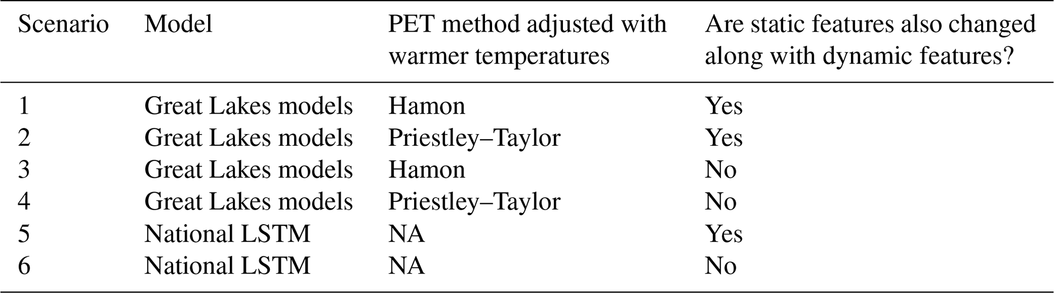
For both the Great Lakes DL models and the national LSTM, the dynamic inputs are adjusted based on the warming scenarios above. We also consider changes to the static input features that depend on temperature and PET in their calculation (e.g., pet_mean, aridity, and t_mean, frac_snow; see Table 1 for feature descriptions and Supporting Information S1 and Table S1 for details on adjustments to these features), and then run all models using two settings: (1) with changes only to the dynamic features and (2) with changes to both dynamic features and to static features that depend on those dynamic features. In total, there are six scenarios run in this work, which are shown in Table 2.

Ultimately, for each model we compare hydrological responses under the warmed scenario to their values under the baseline scenario with no warming. For the national LSTM, we only consider basins in the CAMELS dataset within the Great Lakes Basin. For the process-based models, we also evaluate the uncertainty in hydrological response based on the range predicted across the 10 different training trials, as a simple means to evaluate how parametric uncertainty influences the predictions. We examine four different metrics for this comparison, including

• AVG.Q: the long-term mean of daily streamflow across the entire series;

• FHV: the average of the top 2 % peak flows;

• FLV: the average of the bottom 30 % low flows;

• COM: the median center of mass across all water years, where the center of mass is defined as the day of the water year by which half of the total annual flow has passed.

If our hypothesis is correct that the LSTM cannot distinguish evaporative water loss differences with different PET series but similar warming, whereas process-based and PIML models can, we would expect that under the LSTM using both PET series, long-term mean flow will decline substantially and with similar magnitude to the process-based models using the temperature-based PET method but not the energy-budget-based PET method. We would also expect the national LSTM to exhibit similar behavior, even though it was able to learn from a larger set of watersheds across a more diverse range of climate conditions. Finally, if our hypothesis is correct, we would expect the PIML models (MC-LSTM and MC-LSTM-PET) to follow the process-based model responses more closely across the two different PET series, at least in terms of the difference in magnitude of long-term mean streamflow declines. To facilitate a broader intermodel comparison of DL and process-based models under warming (which is largely absent from the literature), we also explore the differences in low flow (FLV), high flow (FHV), and seasonal timing (COM) metrics across all model versions, where we have less reason to anticipate how DL and process-based models will differ in their responses and across PET formulations. However, for responses like seasonal streamflow timing (COM), we do anticipate that realistic responses should show a shift towards more streamflow earlier in the year, as warmer temperatures lead to more precipitation falling as rain rather than snow and drive snowmelt earlier in the spring.

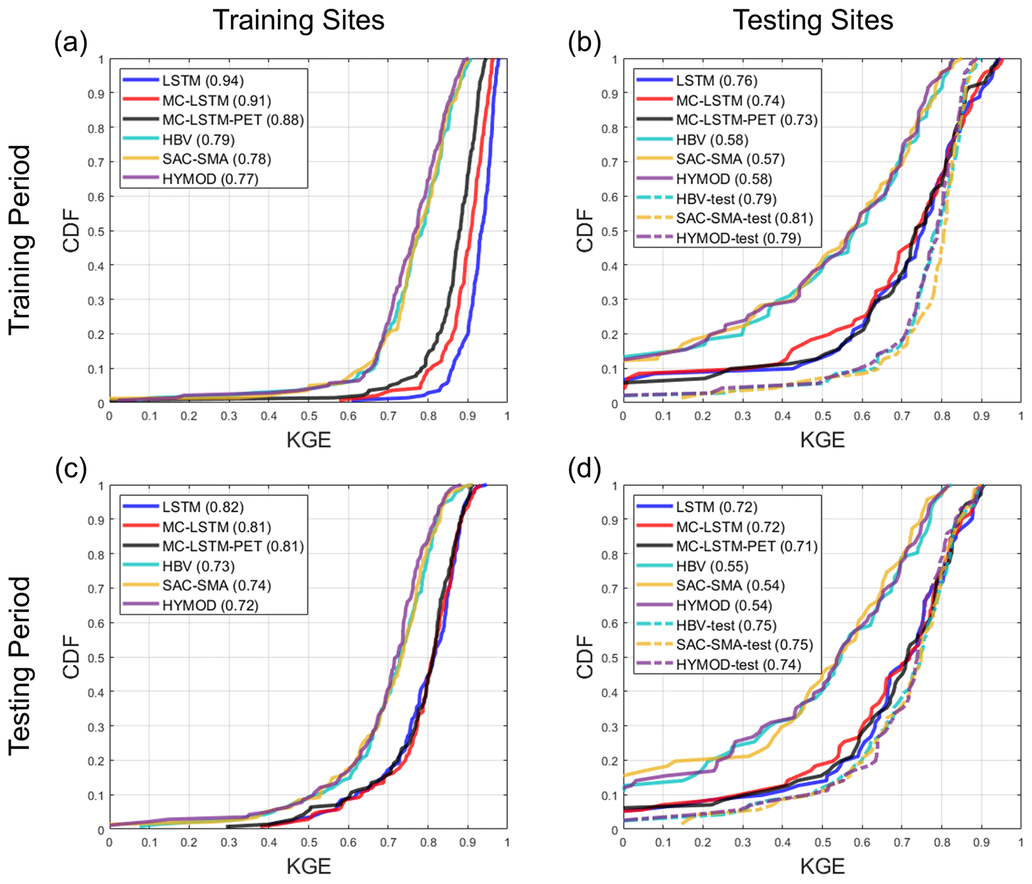
Figure 3 Distribution of the Kling–Gupta efficiency (KGE) for streamflow estimates across sites from each model at the (a) 141 training sites and (b) 71 testing sites for the training period. Similar results for the testing period are shown in (c) and (d), respectively. For the process-based models fit to the testing sites (denoted “-test”), no performance results are available at the training sites. All models are trained using Priestley–Taylor PET.

Table 3 The median KGE, NSE, PBIAS, FHV, and FLV for streamflow across testing sites for the training and testing periods for all models (excluding the process-based models fit to the testing sites). The metric from the best performing model in each period is bolded. All models are trained using Priestley–Taylor PET.

4 Results

4.1 Model performance evaluation

Figure 3 shows the distribution of KGE values across sites for streamflow from the LSTM, MC-LSTM, MC-LSTM-PET, and the three process-based models for both the training and testing sites during both the training and testing periods. All results here and elsewhere in Sect. 4.1 are shown for the models fit with Priestley–Taylor PET, but there is little difference in performance for the models fit with Hamon PET (see Fig. S1 in the Supplement). For the process-based models, we show results for models fit to the training sites and then used as donors at the testing sites, as well as models fit to the testing sites directly. We denote the latter with the suffix “-test” and note that performance metrics at the training sites are not available for process-based models fit to the testing sites.

Several insights emerge from Fig. 3. First, for the training sites during the training period, all models perform very well (Fig. 3a). Across the three process-based models, the median KGE is 0.79, 0.78, and 0.77 for HBV, SAC-SMA, and HYMOD, respectively. However, unsurprisingly, the DL models perform better for the training data, with median KGE values all equal or above 0.88. The LSTM performs best in this case. Under temporal validation (training sites during the testing period), performance degrades somewhat across all models, and the differences in KGE between all process-based models and between all DL models shrink considerably (Fig. 3c). Larger performance declines are seen at the testing sites during the training period (Fig. 3b) and testing period (Fig. 3d). Here, the median KGE for all process-based models falls to between 0.54 and 0.58 when streamflow at the testing sites is estimated with donor models from nearby gauged watersheds. In contrast, process-based models fit to the testing sites (denoted “-test”) exhibit performance similar to that seen in Fig. 3a and c. All three DL models perform quite well for the testing sites, with median KGE values above 0.71 in both time periods. This is only modestly below the median KGE for the process-based models fit to the testing sites, which is quite impressive given that this represents the spatial out-of-sample performance of the DL models. We even see that for approximately 20 % of testing sites during the training period, the DL models outperform the process-based models fit to those locations in that period.

Table 3 shows the median KGE, NSE, PBIAS, FHV, and FLV across testing sites for all models, excluding the process-based models fit to the testing sites. Similar to Fig. 3, all three DL models outperform the donor-based process-based models at the testing sites for all metrics. The performance across the three different DL models is similar, although there are some notable differences. In particular, the LSTM outperforms the MC-LSTM and MC-LSTM-PET for NSE and FLV (as well as KGE in the training period), the MC-LSTM-PET outperforms the LSTM and MC-LSTM for PBIAS, and either the MC-LSTM or MC-LSTM-PET are the best performers for FHV. The fact that the MC-LSTM-PET performs best for PBIAS of all models suggests that the PET constraint imposed in that model improves the overall accounting of water entering and existing the watershed on a long-term basis. We also note that percent biases for FLV are high because the absolute magnitude of low flows is small, so small absolute biases still lead to large percent biases.

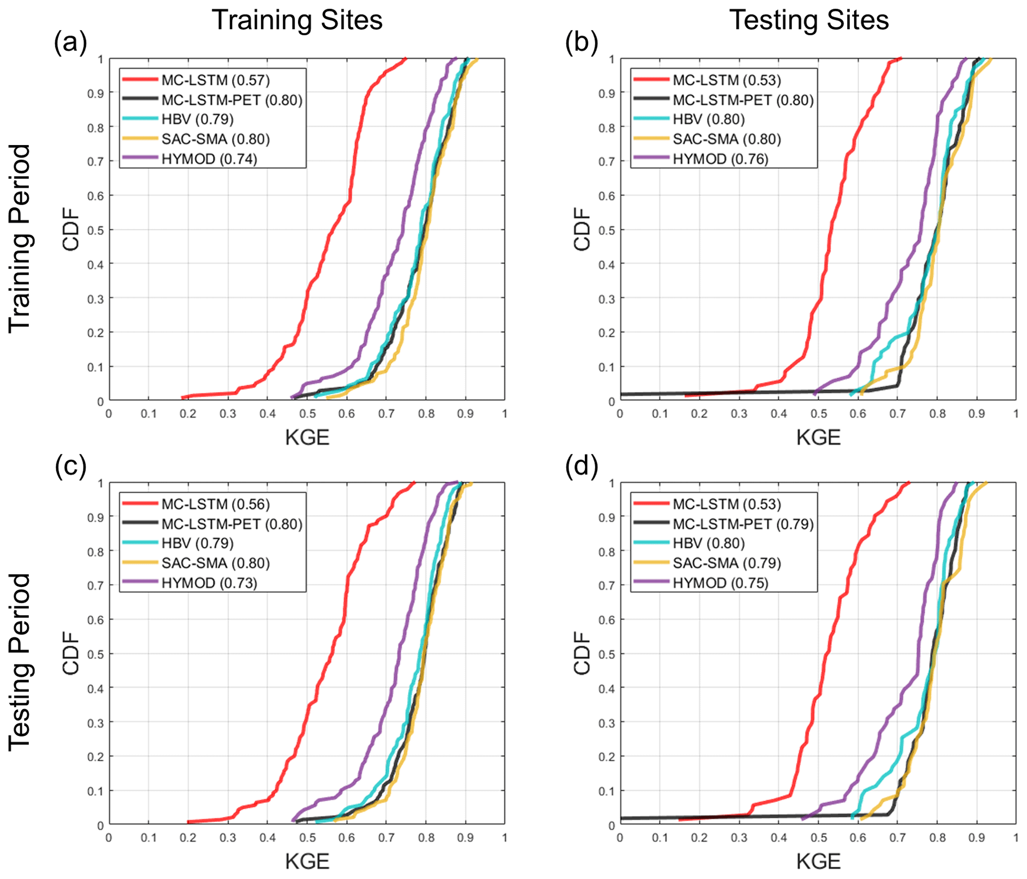
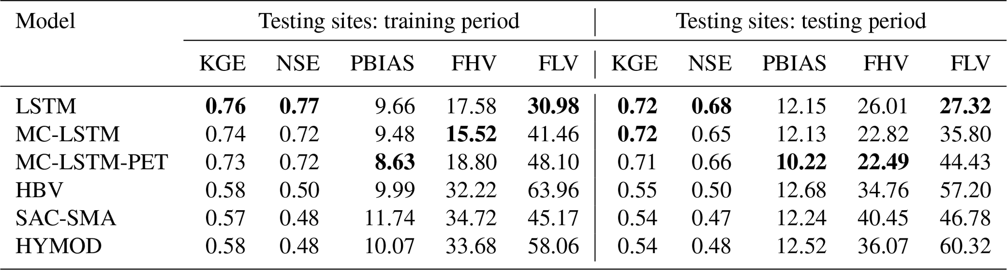
Figure 4 The Kling–Gupta efficiency (KGE) for AET estimated from each model at the (a) 141 training sites and (b) 71 testing sites for the training period. Similar results for the testing period are shown in (c) and (d), respectively. The LSTM is not included in this comparison. All models are trained using Priestley–Taylor PET.

Figure 4 shows similar results as Fig. 3, but for the KGE based on estimates of AET. Also, only donor process-based models are shown for the testing sites. Results for correlation and PBIAS are available in Figs. S2 and S3. Here, the LSTM is not included because estimates of AET are unavailable, while AET from the MC-LSTM and MC-LSTM-PET is based on water relegated to the trash cell. Note that none of the models were trained for AET, and therefore results at training sites during the training period also provide a form of model validation. Figure 4 shows that SAC-SMA and HBV predict AET with relatively high degrees of accuracy for both training and testing sites in both periods (median KGE between 0.79 and 0.80). Performance is slightly worse for HYMOD. Notably, the MC-LSTM-PET exhibits very similar, strong performance for all sites and periods as compared with SAC-SMA and HBV, except for one testing site. In contrast, the MC-LSTM performs the worst of all models, with median KGE values ranging between 0.53 and 0.57.

Figure 5 Scatterplots of daily AET versus trash cell water for the (top) MC-LSTM and (bottom) MC-LSTM-PET at five randomly selected testing sites across both training and testing periods. All models are trained using Priestley–Taylor PET.

Further investigation reveals that the differences in KGE between the MC-LSTM and MC-LSTM-PET models for AET are largely driven by differences in correlation (see Fig. S2). We examine this difference in more detail in Fig. 5, which presents scatterplots of GLEAM AET versus water allocations to the trash cell for the two models from five randomly sampled testing sites across both training and testing periods (see Fig. 1; also see Table S3). Trash cell water from the MC-LSTM is not only more scattered around GLEAM AET compared with the MC-LSTM-PET, but it also exhibits many outlier values that are two to five times larger than GLEAM AET. The MC-LSTM-PET follows the variability of GLEAM AET much more closely, with virtually no outliers that exceed GLEAM AET by large margins. This suggests that the PET constraint on the trash cell in the MC-LSTM-PET helps water allocated to that cell more faithfully represent evaporative water loss in the DL model.

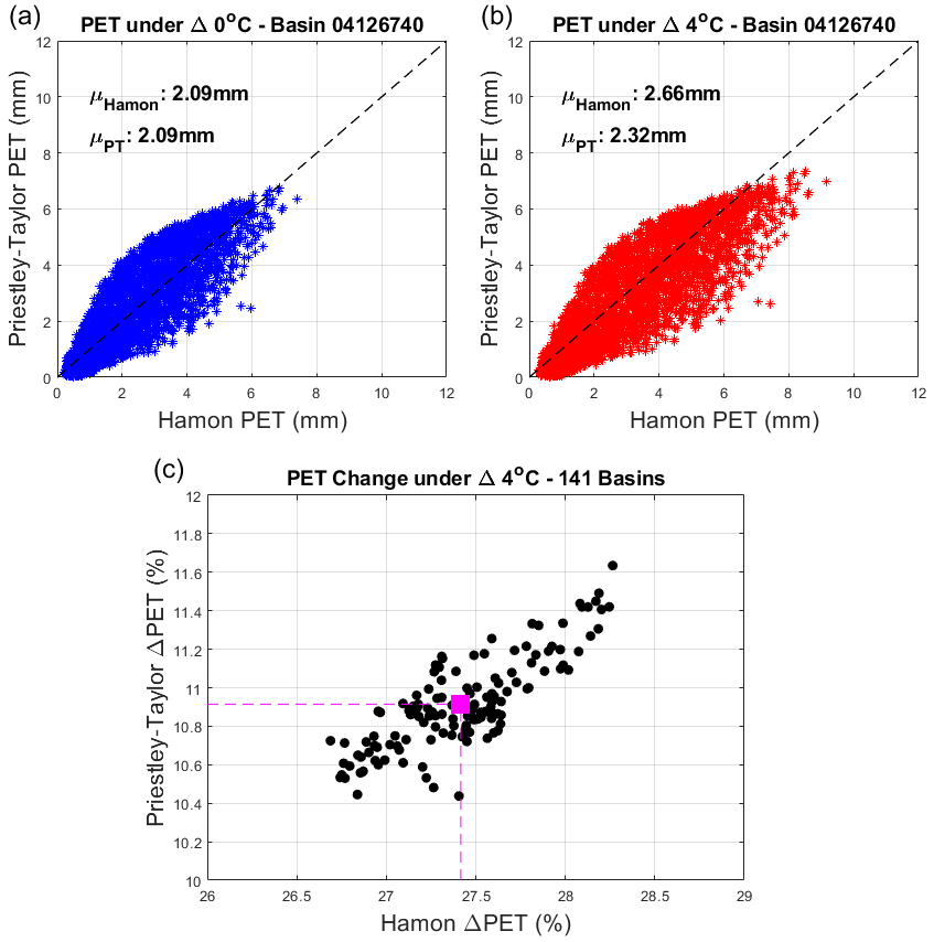
Figure 6 Panel (a) shows daily PET estimated using the Hamon and Priestley–Taylor methods for one sample watershed, under historical climate conditions in the training period. Panel (b) is the same as (a) but under the scenario with 4 ^∘C of warming. Panel (c) shows the percentage of change in average PET with 4 ^∘C of warming across all training sites using the Hamon and Priestley–Taylor methods.

4.2 Evaluating hydrologic response under warming

Next, we evaluate streamflow responses under a 4 ^∘C warming scenario. We focus on training sites during the training period, so that any differences that emerge between DL and process-based models are only related to model structure and not spatiotemporal regionalization. However, our results are largely unchanged if based on responses for testing sites in the testing period (see Fig. S4). First, we show the differences in historical and warming-adjusted PET when using the Hamon and Priestley–Taylor methods (Fig. 6). For the training period without any temperature change, PET estimated from the two methods is very similar (Fig. 6a; shown at one sample location for demonstration, see Fig. 1 and Table S3). However, under the scenario with 4 ^∘C of warming, Hamon-based PET is substantially larger than Priestley–Taylor-based PET (Fig. 6b). On average, this difference reaches ∼ 16 % across all training sites and exhibits very little variability across locations (Fig. 6c). The primary reason for the difference in the estimated change in PET is that the Hamon method attributes PET entirely to temperature, while only a portion of PET is based on temperature in the Priestley–Taylor method, with the rest based on R_n. It is noteworthy that R_n does increase with temperature through its effects on net outgoing longwave radiation, but these changes are generally less than 5 % across all sites (Allen et al., 1998).

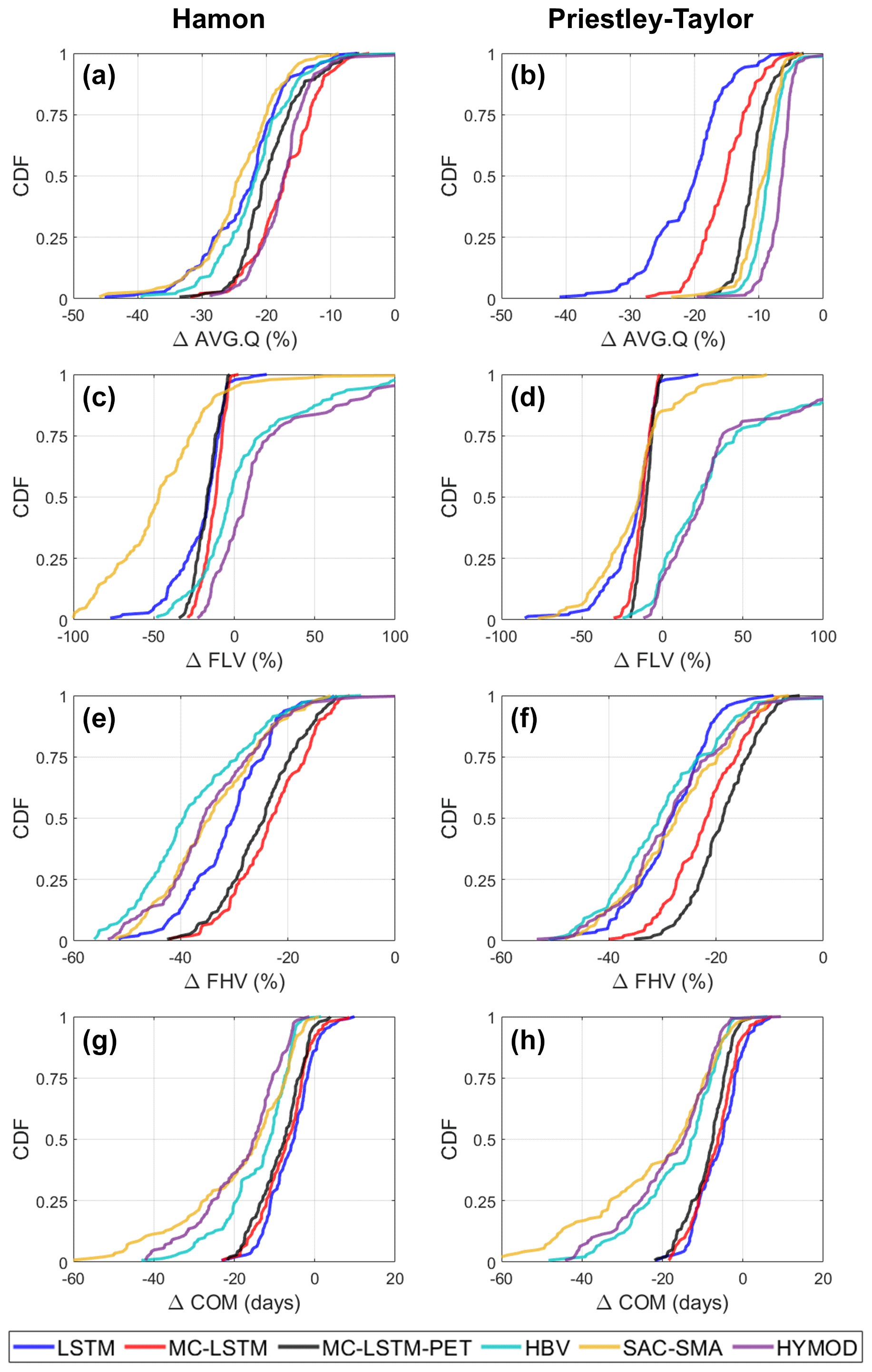
Figure 7 The distribution of change in (a, b) long-term mean daily flow (AVG.Q), (c, d) low flows (FLV), (e, f) high flows (FHV), and (g, h) seasonal streamflow timing (COM) across the 141 training sites and all models under a scenario of 4 ^∘C warming using (a, c, e, g) Hamon PET and (b, d, f, h) Priestley–Taylor PET. For the deep learning models, changes were only made to the dynamic inputs (i.e., no changes to static inputs).

Figure 7 shows how these differences in PET under warming propagate into changes in different attributes of streamflow across training sites in the training period. The left and right columns of Fig. 7 show streamflow responses using Hamon and Priestley–Taylor PET, respectively, while the rows of Fig. 7 show the distribution of changes in different streamflow attributes (AVG.Q, FLV, FHV, and COM) across models. Figure 7 shows results for DL models where only the dynamic inputs are changed under warming.

Starting with changes in AVG.Q, Fig. 7a and b shows that under the Hamon method for PET, the DL models exhibit similar changes in long-term mean streamflow to the process-based models, with the median ΔAVG.Q across sites ranging between −17 % and −25 % across all models. However, when using Priestley–Taylor PET, larger differences in the distribution of ΔAVG.Q emerge. Across all three process-based models, the median ΔAVG.Q is between −6 % and −9 %, and very few locations exhibit ΔAVG.Q less than −20 %. Conversely, the LSTM shows a median water loss of −20 % under Priestley–Taylor PET and a very similar distribution of water losses regardless of whether Hamon or Priestley–Taylor PET was used. The MC-LSTM is also relatively insensitive to PET, and as compared with the process-based models, the MC-LSTM tends to predict smaller absolute changes to AVG.Q for Hamon PET and larger changes under Priestley–Taylor PET. Only the MC-LSTM-PET model achieves water loss that is considerably smaller under Priestley–Taylor PET than Hamon PET and closely follows the process-based models in both cases.

The overall pattern of change in low flows (FLV) is very similar across all three DL models, with median declines between −15 % and −25 % and little variability across sites (Fig. 7c and d). The process-based models disagree on the sign of change for FLV and also bound the changes predicted by the DL models. HBV and HYMOD show mostly increases to FLV under warming and Priestley–Taylor PET, and a mix of increases and decreases across sites for Hamon PET. SAC-SMA exhibits large declines in FLV under warming and Hamon PET, and shows a median change that is similar to the DL models under Priestley–Taylor PET. The percent changes in FLV across models tend to be large because the absolute magnitude of FLV is small, and thus small changes in millimeters of flow lead to large percent changes. This can be seen in sample daily hydrographs for two sites (see Fig. S5), where visually the changes in low flows are difficult to discern because they are all near zero for all models.

The differences between process-based and DL simulated changes for high flows (FHV; Fig. 7e and f) and seasonal timing (COM; Fig. 7g and h) are relatively consistent, with the process-based models exhibiting more substantial declines in high flows and earlier shifts in seasonal timing compared with the DL models. The choice of PET method has an impact on process-model-based changes in FHV, with larger declines under Hamon PET. A similar signal is also seen for the MC-LSTM-PET but not the MC-LSTM or LSTM, although the LSTM predicts changes in FHV closest to the process-based models.

For COM, the process-based models show a wide range of variability in projected change across sites, from no change to 60 d earlier. For the DL models the range of change is much narrower, and the median change in COM is approximately a week less than the median change across the process-based models. The earlier shift in COM across all models is consistent with anticipated changes to snow accumulation and melt dynamics under warming, with more water entering the stream during the winter and early spring as precipitation shifts more towards rainfall and snowpack melts off earlier in the year (Byun and Hamlet, 2018; Mote et al., 2018; Kayastha et al., 2022). However, this effect is seen more dramatically in the process-based models, as evidenced by more prominent changes to their daily and monthly hydrographs under warming during the winter and early spring as compared with the DL models (see Figs. S5 and S6). The method of PET estimation has relatively little impact on both process-based model and DL-based estimates of change in COM.

We note that the results above do not change even when considering the parametric uncertainty in the process-based models, although for some metrics (FLV), uncertainty in process-based model estimated changes due to parametric uncertainty is large (see Fig. S7). We also note that if the static watershed properties (pet_mean, aridity, t_mean, frac_snow; see Table 1) are changed to reflect warmer temperatures and higher PET, all three DL models exhibit unrealistic water gains for 15 %–40 % of locations depending on the model and PET method, with the most water gains occurring under the LSTM (Fig. S8). These results suggest that changing the static watershed properties associated with long-term climate characteristics can degrade the quality of the estimated responses, at least when the temperature shifts are large and the range of average temperature and PET in the training set is limited.

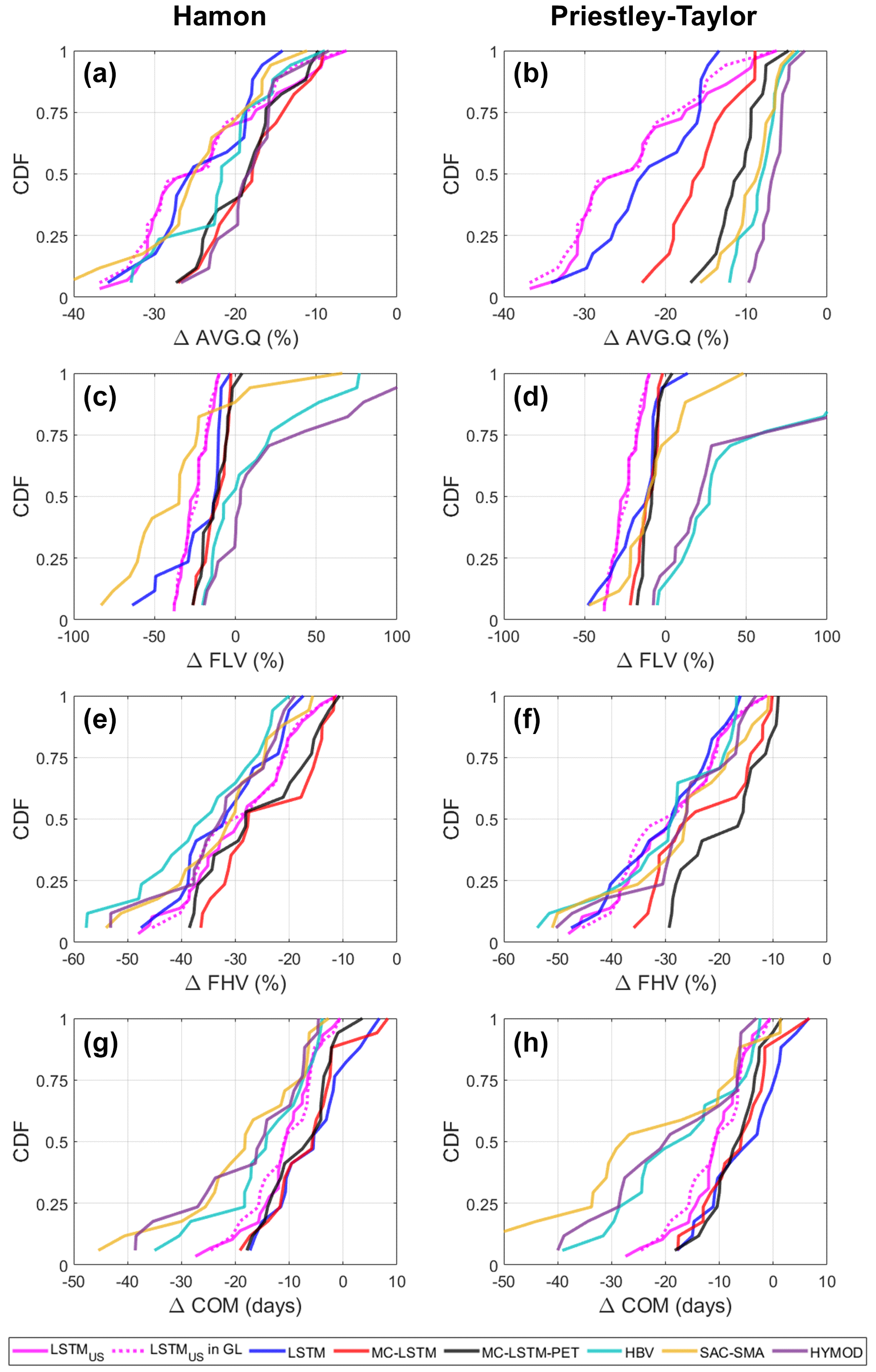
Figure 8 The distribution of change in (a, b) long-term mean daily flow (AVG.Q), (c, d) low flows (FLV), (e, f) high flows (FHV), and (g, h) seasonal streamflow timing (COM) across 29 CAMELS sites within the Great Lakes basin under the national LSTM (solid pink), as well as for 17 of those 29 sites from the Great Lakes deep learning and process-based models, under a scenario of 4 ^∘C warming. Results from the national LSTM for those 17 sites are also highlighted (dashed pink). For the Great Lakes models only, results differ when using (a, c, e, f) Hamon PET and (b, d, f, h) Priestley–Taylor PET. For the national LSTM, changes were made only to the dynamic inputs.

One reason why the Great Lakes LSTM exhibits excessive water losses under warming could be that the model was trained using sites that are confined to a limited range of temperature and PET values found in the Great Lakes basin (spanning approximately 40.5^∘−50^∘ N), and therefore it is ill-suited to extrapolate hydrological response under warming conditions that extend beyond this temperature and PET range. To evaluate this hypothesis, we examine changes to AVG.Q, FLV, FHV, and COM under 4 ^∘C warming at the 29 CAMELS watersheds within the Great Lakes basin using the national LSTM (Fig. 8). For comparison, we also examine similar changes under all six Great Lakes DL and process-based models at 17 of those 29 CAMELS basins that were used in the training and testing sets for the Great Lakes models. We also highlight the national LSTM predictions for those 17 sites. Note that in Fig. 8, the national LSTM predictions do not differ between Hamon and Priestley–Taylor PET, because PET is not an input to that model.

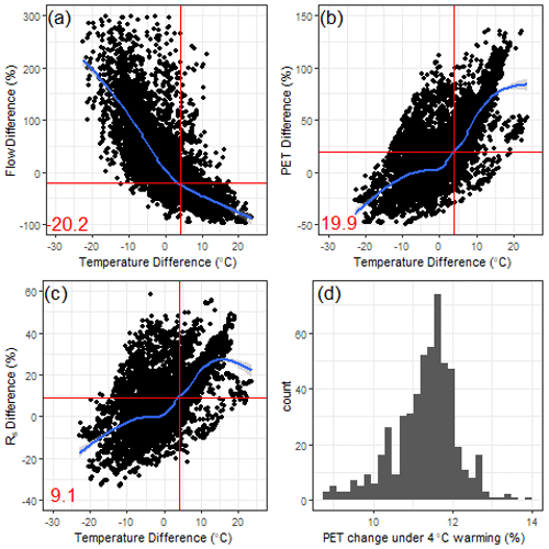
Figure 9 The percent difference in long-term (1980–2014) mean (a) streamflow, (b) Priestley–Taylor-based PET, and (c) downward shortwave radiation (R_s) for all pairs of CAMELS basins with average precipitation within 1 % of each other, plotted against differences in average temperature for each pair. A loess smooth is provided for each scatter (blue), along with the changes in variable estimated at a 4 ^∘C temperature difference between pairs of sites (red). Panel (d) shows the projected change in Priestley–Taylor-based PET (as a percentage) for each CAMELS basin under 4 ^∘C warming, assuming no change in R_s.

The national LSTM was trained to watersheds across the CONUS (spanning approximately 26–49^∘ N) and thus was exposed to watersheds with much warmer conditions and higher PET during training. However, we find that the national LSTM still predicts very large declines in AVG.Q. For the 29 CAMELS watersheds in the Great Lakes basin, the median decline in AVG.Q under the national LSTM is approximately 25 %, which is only 0 %–6 % larger than the median predictions of loss under the process-based models using Hamon PET but 16 %–19 % larger than the process-based model losses under Priestley–Taylor PET (Fig. 8a and b). We also see larger declines in FLV under the national LSTM as compared with the other Great Lakes DL models (Fig. 8c and d). The national LSTM predicts changes in FHV (Fig. 8e and f) and COM (Fig. 8g and h) that are relatively similar to the process-based models. For COM, the predictions of change are still smaller than the process-based models but closer to the process-based models than any Great Lakes DL model, suggesting that the national LSTM predicts shifting snow accumulation and melt dynamics more consistently with the process-based models than regionally fit DL models. In addition, the hydrological predictions are stable under the national LSTM regardless of whether only dynamic inputs or both dynamic and static inputs are changed under warming (see Fig. S9), in contrast to the Great Lakes DL models. Therefore, the use of more watersheds in training that span a more diverse set of climate conditions likely benefits the model when inputs are shifted to reflect new climate conditions. However, as shown in Fig. 8a and b, this benefit does not mitigate the tendency for the national LSTM to overestimate water loss under warming.

To better understand why the national LSTM predicts large water losses under warming, it is instructive to examine how long-term mean streamflow, (Priestly–Taylor estimated) PET, and R_s vary across all 531 CAMELS watersheds of different average temperatures, and compare this variability to predicted changes in PET at each site under warming. Specifically, we calculate the difference in long-term (1980–2014) mean streamflow (Fig. 9a), PET (Fig. 9b), and R_s (Fig. 9c) across all pairs of basins in the CAMELS dataset with average long-term precipitation within 1 % of each other (i.e., we only examine pairs of basins with very similar long-term mean precipitation). Then, for each basin pair, we plot the difference in long-term mean streamflow, PET, and R_s against the difference in long-term average temperature for that pair. The results show that the difference in long-term mean streamflow across watersheds with similar precipitation becomes negative when the difference in temperature is positive (i.e., warmer watersheds have less flow on average), and that when the difference in average temperature reaches 4 ^∘C, flows differ by about 20 % on average (Fig. 9a). This is very similar to the predicted median decline in long-term mean streamflow seen for the national LSTM in Fig. 8. We also note that average PET increases by approximately 20 % between watersheds that differ in average temperature by 4 ^∘C (Fig. 9b). However, higher PET in warmer watersheds is related both to the direct effect of temperature on vapor pressure deficit as well as to the fact that higher incoming solar radiation co-occurs in warmer watersheds (R_s is approximately 9 % higher across watershed pairs that differ by 4 ^∘C; Fig. 9c). Using the Priestley–Taylor method, we estimate that average PET would only increase by 9 %–14 % (median of 11.5 %) if temperatures warm by 4 ^∘C and R_s is held at historical values, while R_n is increased slightly due to declines in net outgoing longwave radiation with warming (Fig. 9d). However, the national LSTM appears to convolute the effects of temperature and R_s and cannot separate out their effects on evaporative water loss, leading to larger predicted streamflow losses under 4 ^∘C warming than changes in PET would warrant. This is possibly because of the very strong correlation between at-site daily temperature and R_s historically (median correlation of 0.85 across all CAMELS watersheds).

5 Discussion and conclusion

In this study, we contribute a sensitivity analysis that evaluates the physical plausibility of streamflow responses under warming using DL rainfall–runoff models. The basis for this evaluation is anchored to the assumption that differences in estimated streamflow responses should emerge under very different scenarios of PET under warming, and that realistic predictions of PET and water loss under warming tend to be much lower than those estimated by temperature-based PET methods. Accordingly, we assume that physically plausible streamflow predictions should be able to respond to lower energy-budget-based PET projections under warming and, all else being equal, estimate smaller streamflow losses.

The results of this study show that a standard LSTM did not predict physically realistic differences in streamflow response across substantially different estimates of PET under warming. This discrepancy emerged despite the fact that the standard LSTM was a far better model for streamflow estimation in ungauged basins compared with three process-based models under historical climate conditions. In addition, the national LSTM trained to a much larger set of watersheds (531 basins across 23^∘ of latitude) using temperature, vapor pressure, and R_s directly (rather than PET) also estimated water loss under warming that far exceeded the losses estimated with process-based models forced with energy-budget-based PET. Since water losses estimated using energy-budget-based PET are generally considered more realistic (Lofgren et al., 2011; Shaw and Riha, 2011; Lofgren and Rouhana, 2016; Milly and Dunne, 2017; Lemaitre-Basset et al., 2022), this result casts doubt over the physical plausibility of the LSTM predictions produced in this work.

Results from this work also suggest that PIML-based DL models can capture physically plausible streamflow responses under warming while still maintaining superior prediction skill compared with process-based models, at least in some cases. In particular, a mass conserving LSTM that also respected the limits of water loss due to evapotranspiration (the MC-LSTM-PET) was able to predict changes in long-term mean streamflow that much more closely aligned with process-model-based estimates while also providing competitive out-of-sample performance across all models considered (including the other DL models). A more conventional MC-LSTM that did not limit water losses by PET was less consistent with process-based estimates of change in long-term mean streamflow. These results highlight the potential for PIML-based DL models to help achieve similar performance improvements over process-based models as documented in recent work on DL rainfall–runoff models (Kratzert et al., 2019a, b; Feng et al., 2020; Nearing et al., 2021) while also producing projections under climate change that are more consistent with theory than non-PIML DL models.

An interesting result from this study was the disagreement in the change in high flows and seasonal streamflow timing between all Great Lakes DL models and process-based models, the latter of which estimated greater reductions in high flows and larger shifts of water towards earlier in the year. Predictions from the Great Lakes DL models were also unstable if static climate properties of each watershed were changed under warming. In contrast, the national LSTM was more stable if static properties were changed, and it predicted changes to high flows and seasonal timing that were more like the process-based models than predictions from the Great Lakes DL models. The results for COM in particular suggest that the national LSTM may be more consistent with the process-based models in terms of its representation of warming effects on snow accumulation and melt processes and the resulting shifts in the seasonal hydrograph, although differences with the process-based model predictions were still notable. Still, these results are consistent with past work showing that large-sample LSTMs can learn to represent snow processes internally from meteorological and streamflow data (Lees et al., 2022). While it is challenging to know which set of predictions are correct for these streamflow properties, these results overall favor predictions from the national LSTM over the regional LSTMs and highlight the benefits of DL rainfall–runoff models trained to a larger set of diverse watersheds for climate change analysis.

To properly interpret the results of this work, there are several limitations of this study that require discussion. First there were differences in the inputs and data sources between the national LSTM and all other Great Lakes models, including the source of meteorological data and the lack of PET as an input into the national LSTM. While the national LSTM was provided meteorological inputs that together completely determine Hamon and Priestley–Taylor PET, the difference in meteorological data across the two sets of models is a substantial source of uncertainty and could lead to non-trivial differences in hydrological response estimation, complicating a direct comparison of the national LSTM to the other models. Future work for the Great Lakes Intercomparison Project should consider developing consistent datasets with other (and larger) benchmark datasets like CAMELS to address this issue.

Another important limitation is how we constructed the warming scenarios, with 4 ^∘C warming and shifts to PET but no changes to other meteorological variables (net incoming shortwave radiation, precipitation, humidity, air pressure, and wind speeds). These scenarios and associated sensitivity analyses were constructed in the style of other metamorphic tests for hydrological models (Yang and Chui, 2021; Razavi, 2021; Reichert et al., 2023), where we define input changes with expected responses and test whether model behavior is consistent with these expectations. However, for DL and other machine learning models, the results of such sensitivity analyses may be unreliable because of distributional shifts between the training and testing data and poor out-of-distribution generalization (see Shen et al., 2021, Wang et al., 2023, and references therein). When trained, conventional machine learning models try to leverage all of the correlations within the training set to minimize training errors, which is effective in out-of-sample performance only if those same patterns of correlation persist into the testing data (Liu et al., 2021). In our experimental design, we impose a distinct shift in the joint distribution of the inputs (i.e., a covariate shift) by increasing temperatures and PET but leaving unchanged other meteorological inputs, thereby altering the correlation among inputs. Therefore, one might expect some degradation in the DL-model-based predictions of streamflow under these scenarios.

The challenge of out-of-distribution generalization and its application to DL rainfall–runoff model testing under climate change highlights several important avenues for future work. First, additional efforts are needed to evaluate the physical plausibility of DL-based hydrological projections under climate change while ensuring that the joint distribution of all meteorological inputs used in future scenarios is realistic. For example, there are physical relationships between changes in temperature and net radiation (Nordling et al., 2021), as well as temperature, humidity, and extreme precipitation (Ali et al., 2018; Najibi et al., 2022), that should all be preserved in future climate scenarios. The use of climate model output may be well suited for such tests, although care is needed to avoid statistical bias correction and downscaling (i.e., post-processing) of multiple climate fields that could cause shifts in the joint distribution across inputs (Maraun, 2016). High-resolution convective-permitting models may be helpful in this regard, given their improved accuracy for key climate fields like precipitation (Kendon et al., 2017).

There are also several emerging techniques in machine learning to address out-of-distribution generalization directly. One set of promising methods is causal learning, defined broadly as methods aimed at identifying input variables that have a causal relationship with the target variable and to leverage those inputs for prediction (Shen et al., 2021). PIML approaches, such as the MC-LSTM-PET model proposed in this work, fall into this category (Vasudevan et al., 2021). Here, prior scientific knowledge on causal structures can be embedded into the DL model through tailored loss functions or, as in the case of the MC-LSTM-PET model, through architectural adjustments or constraints. (For other examples outside of hydrology, see Lin et al., 2017; Ma et al., 2018.) The MC-LSTM-PET model can be viewed as a specific, limited case of a broader class of learnable, differentiable, process-based models (also referred to as hybrid differentiable models; Jiang et al., 2020; Feng et al., 2022, 2023a). These models use process-based model architectures as a backbone for model structure, which is then enhanced through flexible, data-driven learning for a subset of processes. Recent work has shown that these models can achieve similar performance to LSTMs but can also represent and output different internal hydrological fluxes (Feng et al., 2022, 2023a).

However, challenges can arise when imposing architectural constraints in PIML models. For example, the MC-LSTM-PET model makes the assumption that all water loss in the system is due to evapotranspiration and therefore cannot exceed PET. However, other terminal sinks are possible, such as human water extractions and interbasin transfers (Siddik et al., 2023) or water lost to aquifer recharge and interbasin groundwater fluxes (Safeeq et al., 2021; Jasechko et al., 2021). It is difficult to know the magnitude of these alternative sinks given unknown systematic errors in other inputs (e.g., underestimation of precipitation from under-catch) that confound water balance closure analyses. Still, recent techniques and datasets to help quantify these sinks (Gordon et al., 2022; Siddik et al., 2023) provide an avenue to integrate them into the MC-LSTM-PET constraints. Yet as constraints are added to the model architecture, the potential grows for inductive bias that negatively impacts generalizability. For instance, a recent evaluation of hybrid differentiable models showed that they underperformed relative to a standard LSTM due to structural deficiencies in cold regions, arid regions, and basins with considerable anthropogenic impacts (Feng et al., 2023b). Some of these challenges may be difficult to address because only differentiable process-based models can be considered in this hybrid framework, limiting the process-based model structures that could be adapted with this approach. Additional work is needed to evaluate the benefits and drawbacks of these different PIML-based approaches, preferably on large benchmarking datasets such as CAMELS or CAVARAN (Kratzert et al., 2023).

Given some of the potential challenges above, other DL methods that make use of causal concepts while making fewer assumptions on watershed-scale process controls are also worth pursuing. For example, a series of techniques have emerged that embed the concept and constraints of directed acyclic graphs within deep neural networks in such a way that the architecture of the neural network is inferred from the data to encode causality among variables (see Luo et al., 2020, and references therein), that is, frameworks to optimize the architecture of the model can be designed not only to maximize out-of-sample predictive performance but also to promote causality. Alternatively, domain-invariant learning attempts to promote the identification of features that are domain specific versus domain invariant by separating and labeling training data from different “domains” or “environments” (Ilse et al., 2021). In the case of DL rainfall–runoff models, this strategy could be implemented, for instance, by pairing observed climate and streamflow (one domain) with land-surface-model-based streamflow estimated using future projected climate model output (another domain), with the goal of learning invariant relationships between key climate inputs (e.g., net radiation or PET) and streamflow across the two domains. Here, there may be a benefit of including data from the land surface and climate models, where the correlation between temperature, net radiation, and PET may be weaker under projected climate change. These techniques offer an intriguing alternative for the next generation of DL hydrological models that can generalize well under climate change and should be the focus of further exploration.