Technical note: A guide to using three open-source quality control algorithms for rainfall data from personal weather stations

The number of rainfall observations from personal weather stations (PWSs) has increased significantly over the past years; however, there are persistent questions about data quality. In this paper, we reflect on three quality control algorithms (PWSQC, PWS-pyQC, and GSDR-QC) designed for the quality control (QC) of rainfall data. Technical and operational guidelines are provided to help interested users in finding the most appropriate QC to apply for their use case. All three algorithms can be accessed within the OpenSense sandbox where users can run the code. The results show that all three algorithms improve PWS data quality when cross-referenced against a rain radar data product. The considered algorithms have different strengths and weaknesses depending on the PWS and official data availability, making it inadvisable to recommend one over another without carefully considering the specific setting. The authors highlight a need for further objective quantitative benchmarking of QC algorithms. This requires freely available test datasets representing a range of environments, gauge densities, and weather patterns.

1 Introduction

Precipitation is highly variable in space and time; thus, the accurate estimation of precipitation amounts is of fundamental importance for many hydrological purposes (Estévez et al., 2011), especially on smaller scales and high temporal resolutions such as in small catchments and in the field of urban hydrology (Berne et al., 2004; Ochoa-Rodriguez et al., 2015; Cristiano et al., 2017), where typical rain gauge networks are not always sufficiently dense to capture the spatio-temporal variability of precipitation. Weather radar provides rainfall estimates with good spatial coverage, but since radar is an indirect measurement, its data suffer from errors and uncertainties (Fabry, 2015; Rauber and Nesbitt, 2018). One approach to improve precipitation estimates is the use of additional data from so-called opportunistic sensors (OSs) such as terrestrial commercial microwave links, personal weather stations (PWSs), or satellite microwave links, which are typically more numerous than rain gauges from national weather services. The high number of OS devices offers a huge potential to better capture the strong spatio-temporal variability of rainfall, especially in regions with scarce conventional meteorological observations. This holds true in particular for PWSs, where the number of stations has increased considerably over the last years.

Some of the most popular and widely available PWSs are simple, low-cost instruments that measure various meteorological parameters, including temperature, wind, and rainfall. The rain gauges of PWSs are typically unheated tipping-bucket gauges with varying orifice sizes and measurement resolutions. Operators of PWSs also have the opportunity to share and visualize the data on online platforms. For further details on PWSs and PWS networks, see de Vos et al. (2019) and Fencl et al. (2024).

Since these PWSs may be installed by people who do not have access to, or knowledge of, optimal gauge placement, it is expected that many of these stations are not set up and maintained according to professional standards. Furthermore, issues like uncertain or missing metadata, data gaps, variable time steps, and biases are frequent and hamper the use of PWS rainfall data for hydrological and meteorological applications (de Vos et al., 2019; O'Hara et al., 2023). Overall, there is a high availability of PWS data, but the expected quality of these data is fairly low.

As with all weather observations, in order to make constructive use of PWS rainfall observations, the application of reliable quality control (QC) is vital. Many national meteorological services and other institutions have operational QC algorithms for their precipitation data, but these are typically not open source and are not tailored for PWS data. This can be because they assume a higher data availability and smaller bias than what is commonly found from PWS devices. In the past years, several QC methods for PWS rainfall data have been proposed, which are typically applied to PWS datasets in different geographical areas or time periods. This lack of overlap in climate, conditions, and network density can make it difficult for a reader to compare these methods. Overcoming these limitations and making these data from PWSs and other OSs available to a broader scientific community are aims of the EU COST Action CA2016 “Opportunistic Precipitation Sensing Network (OpenSense)” (https://opensenseaction.eu/, last access: 14 October 2024), where, for example, data standards (Fencl et al., 2024) and software for processing and quality controlling OS data (https://github.com/OpenSenseAction/OPENSENSE_sandbox, last access: 14 October 2024) are being developed.

For people new to the field, it can be difficult to appreciate the differences between the available methods and decide on which method best suits their needs. The aim of this paper is to provide a guideline to using three different open-source QC methods designed especially for precipitation data. They can be run in the public sandbox environment of the OpenSense EU COST Action (https://github.com/OpenSenseAction/OPENSENSE_sandbox). As an example, the methods are applied to the same publicly available PWS rainfall dataset from the Amsterdam metropolitan area in the Netherlands. Lastly, by following the open-data and open-source concepts, the implementation of the QC algorithms is reproducible. The OpenSense COST Action strives to promote FAIR (Findability, Accessibility, Interoperability, and Reuse) principles in research, which are increasingly adopted and required by publishers, funding agencies, and academic institutions (Boeckhout et al., 2018).

This paper is structured as follows. Section 2 describes and compares the three different QC methods. Section 3 provides instructions and guidelines on how to run these QC methods in the OpenSense sandbox environment. In Sect. 4, a case study where these QC methods have been applied using a PWS dataset from the Amsterdam region in the Netherlands is presented. This is followed by a discussion and conclusions and recommendations for the usage of these QC methods in Sects. 5 and 6, respectively.

2 Description of the QC algorithms

2.1 PWSQC

PWSQC was originally developed and published by de Vos et al. (2019). It consists of several QC modules, all relying on neighbour checks. Neighbours are defined as all PWSs within a spatial range, which is a parameterized value. The range should reflect the distance over which one assumes neighbouring PWSs to capture similar rainfall dynamics. This value needs to be chosen carefully for the local climate and the temporal resolution of the PWS data, as the rainfall fields corresponding to longer time steps are more homogeneous than those from short time steps (Terink et al., 2018). For high temporal resolution PWS data, neighbour comparisons can only be sensible if neighbour PWSs are selected with a short range. As the selection is only based on distance, local effects like elevation or land use are ignored. Another parameter in the method sets the required minimum number of neighbouring PWSs that provide observations each time step to ensure that the neighbour comparison is robust. When this parameter is chosen too high, the minimum number of neighbour observations is never reached in sparse areas of the network.

A faulty zero (FZ) filter checks for periods of 0 mm rainfall where the median of nearby PWS observations is above zero. The high influx (HI) filter detects unrealistically high measurements compared to its surroundings by comparing values against the median of its neighbouring PWSs, with a fixed threshold for low rainfall intensities and a dynamic high threshold during rainfall events (as measured by nearby PWSs). The station outlier (SO) check calculates the correlation between a PWS and each neighbouring PWS and starts flagging when the correlation of most becomes too low. Finally, a dynamic bias correction factor (which differs for each PWS and can change in time) is calculated and applied to the observations. For the initial value of the bias correction factor, an auxiliary dataset can be considered to derive a proxy for the overall bias of the whole dataset. This will improve the results, but no auxiliary data are required for the application of PWSQC. The method attributes flags to individual observations that can then be filtered; it does not exclude complete time series. PWSQC has originally been applied on the same dataset as the one used in this paper and showed promising results. The method has been implemented in R and is openly available (de Vos, 2021). Later, a radar version of this algorithm has been constructed in Python that makes use of unadjusted radar data at the location of a PWS as input for the QC. Then neighbouring PWSs are only employed to improve the radar input data (Van Andel, 2021).

2.2 PWS-pyQC

PWS-pyQC was first introduced by Bárdossy et al. (2021). It was used in a study in Germany in Graf et al. (2021) and an event-based analysis in Bárdossy et al. (2022), showing the potential of PWS data to improve precipitation interpolation. The method is implemented in Python and is open-source software available via El Hachem (2022). The QC algorithm consists of three main modules. The first identifies reliable PWSs using a space-time dependence structure derived from a reference observation network (denoted as the primary network). The main assumption is that the PWS values might be wrong but their relative orders (i.e. their ranks) are correct. First, the indicator correlation values are calculated from the reference network and the PWS observation series individually. Each time series is transformed into a binary series depending on the corresponding precipitation value ($z=F^{-\mathrm{1}}\left(\mathit{\alpha }\right)$) for the selected quantile value (α), which has to be chosen depending on the temporal resolution of the data (see Bárdossy et al., 2021). For hourly values, the indicator series are obtained by using a threshold of α=0.99. After deriving the pair-wise indicator correlation matrix from the reference network, the PWS data can be filtered. For each PWS, the indicator correlation with the nearest neighbouring primary station is calculated and compared, for the same separating distance, to the corresponding value in the reference correlation matrix. This allows for identifying and filtering PWS observation series that do not fit in the reference correlation structure. An advantage of using indicator correlations is that the absolute values do not matter (e.g. if 50 and 10 mm both exceed the threshold ($z=F^{-\mathrm{1}}\left(\mathit{\alpha }\right))$, they are both transformed to the value of 1). Furthermore, stations with incorrect location information can be identified as well. A disadvantage of this approach is that the complete time series of the corresponding PWS is disregarded and filtered out.

The second module corrects the bias in the magnitudes of the values of each PWS individually using the ranks of the PWSs and the corresponding neighbouring primary observations. To that end, for every PWS value larger than 0 mm, its corresponding rank and subsequent quantile are identified. For the same quantile level, the corresponding precipitation values at the nearest primary stations are identified. These are then used to interpolate the precipitation value at the PWS location. This corrects the bias in the PWS values individually while preserving their ranks. It is the most time-consuming part of PWS-pyQC as each hourly value has to be individually corrected.

The third module is an event-based filter to identify erroneous PWS observations (false zeros, false extremes) for corresponding time intervals. The filter is based on a leave-one-out cross-validation approach. After applying a Box–Cox transformation to transform the PWS and primary data, each PWS value (after bias correction) is removed from the dataset and is re-estimated using the observation from the primary network. The ratio between the absolute difference of the estimated and observed values and the kriging estimation variance is noted. Large ratios indicate that the observation is an outlier (a single value or a false measurement). Depending on the magnitude of the flagged observation (zero or high precipitation value), the user has to decide to keep or disregard the value. For this step, external information such as weather radar data or discharge value (for headwater catchments) could be used to distinguish between a false measurement and a single event. Note that this filter was further developed in El Hachem et al. (2022).

PWS-pyQC relies on a reference network (a primary network) with reliable observations to filter the PWS data. This is usually acquired from the official rain gauge network. However, in the study area, there is only one KNMI rain gauge with hourly temporal resolution available, which is not sufficient for deriving a reference dependence structure. Hence, this dependence structure was derived from a radar gauge-adjusted KNMI product by taking the time series of 20 randomly chosen pixels as the primary network. A sensitivity analysis will help determine what the impact might be when 20 other pixels (or even a different number of pixels) are chosen as a primary network proxy. If an official rain gauge network is available with enough gauges within the study area, it is recommended to use it.

2.3 GSDR-QC

GSDR-QC is the QC algorithm developed to construct the “Global SubDaily Rainfall” dataset (Lewis et al., 2019) and is fully described in Lewis et al. (2021). The algorithm flags and removes suspicious individual observations rather than entire gauge datasets, and it does not attempt to alter (bias correct) observations, making it the most conservative of the QC methods described herein. GSDR-QC applies user-defined thresholds for hourly and daily maximum rainfall (appropriate to the extent of the study area), conducts nearest-neighbour checks, and uses climate indices defined by the Expert Team on Climate Change Detection Indices (ETCCDI, https://www.ecad.eu/indicesextremes/, last access: 14 October 2024), comprising R99p, PCPTOT, Rx1day, CDD, and SDII. These are described in Table 1 of Lewis et al. (2021). The outputs of GSDR-QC allow the user to evaluate QC summary overviews to establish where faults lie, offering insight into the type of errors.

The complete procedure relies on a two-step process: first flagging suspicious observations, followed by the application of a rule base that uses the flags to remove unreliable observations. The process is comprehensive, addressing all World Meteorological Organization (WMO) tests recommended for rainfall QC: format, completeness, consistency, tolerance/range, and spike and streak (WMO, 2021). A reference table describing each test is presented in the supplementary information of Villalobos‐Herrera et al. (2022). There are 25 QC checks that flag suspicious data: QC1–QC7 that identify where a substantial portion of the gauge data appear to be suspicious (i.e. the gauge is seemingly unreliable), QC8–QC11 that flag suspiciously high values, QC12 that flags long periods without rainfall, and QC13–QC15 that flag suspect accumulations or repeated values. Checks QC8, QC9, and QC11–QC15 use ETCCDI indices as reference data (QC10 implements the user-defined maximum rainfall values). There are, then, further QC flags applied based on observations from neighbouring gauges, including QC16–QC25 that flag mismatches between neighbours including high rainfall, dry periods, and the timing of rainfall. In the original implementation, three of these checks require access to the restricted-access Global Precipitation Climatology Centre (GPCC) daily and monthly precipitation databases; however, these are not essential and are not used in this local implementation of the GSDR-QC algorithm (as applied herein).

Once data have been flagged, a rule base uses 8 of the 25 QC checks to determine suspicious observations which are removed from the dataset. Briefly, the rule base applies the QC checks against neighbouring gauges (×2), for extremely large values (×2), for long dry spells, for repeated non-zero values, and for suspect daily and monthly accumulations. Table 3 in Lewis et al. (2021) provides a full description of the rule base. A key aspect of the neighbour checks is that they are applied to an aggregated daily total to avoid any potential issue caused by the higher variability and intermittency of hourly rainfall (Lewis et al., 2021). This variability and intermittency tend to be higher in data originating from official networks (the original application of GSDR-QC) since they are much less dense than PWS networks, especially in urban areas (O'Hara et al., 2023).

GSDR-QC can be tailored to the dataset/location in many ways. The most obvious adjustments are defining appropriate maximum hourly and daily thresholds for rain (required for the extreme value checks) and determining nearest neighbours. In our case study, we opted for hourly maximum (90.7 mm) and daily maximum (131.7 mm) rainfall data that were representative of the climate of the study area. We allowed an intercomparison of up to 10 nearest neighbours that were within a 50 km radius and had a minimum of 1 year of overlapping data.

2.4 Overview of QC technical and operational guidelines

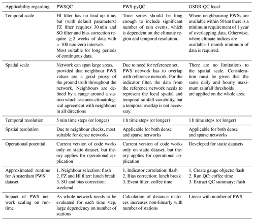
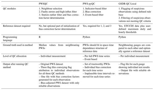
Table 1 recaps the technical differences between the three QC methods. Table 2 offers those interested in applying QC on PWS data an overview on the applicability of the three different QC methods, thus supporting them in choosing the most suitable QC method for processing specific datasets (time series length, temporal resolution, PWS network density, etc.), the availability of a reference dataset, and computational resources.

Table 1 Technical overview of the QC algorithms.

QC methods are available in the OpenSense sandbox (https://github.com/OpenSenseAction/OPENSENSE_sandbox).

Table 2 Operational guidelines for the use of the QC algorithms.

3 Getting started in the sandbox

All three QC algorithms are available under https://github.com/OpenSenseAction/OPENSENSE_sandbox, which is the OpenSense GitHub repository. This repository includes a binder which allows users to run and explore the code online as well as instructions on how to install the environment locally. It is not required to have a GitHub account.

The version of the PWSQC code available in the OpenSense sandbox (https://github.com/OpenSenseAction/OPENSENSE_sandbox/tree/main/PWSQC_R_notebook, last access: 14 October 2024) is practically identical to the originally published R code, with an added introduction to download a PWS dataset directly from the internet repository and save it in the correct format to get started. The code runs in an R kernel, and all steps are listed in two Jupyter Notebook instances. Due to the time it takes the code to run in the sandbox, particularly the step with the SO filter and the dynamic bias correction factor calculation, users may explore the minimal example first, where 10 time series in the PWS dataset are attributed FZ and HI flags only and where the results are visualized.

The PWS-pyQC repository includes a folder with a Jupyter Notebook showcasing the workflow of the algorithm with the Amsterdam PWS dataset. After the import of the modules which include the code for the PWS-pyQC modules in the file PWSpyqcFunctions.py, some user-specific settings like the maximum distance for which the indicator correlation is calculated or the threshold percentile for the indicator correlation can be made. The user can set or change the three parameter values of the QC, which need to be adjusted according to the temporal resolution of the data and the network density. The sample data can be loaded, and the notebook then produces several plots showing the locations of the primary stations and PWSs. This is followed by examples for the different filters. The indicator filter accepts and rejects PWSs that do not match the spatial correlation pattern of the reference network. The bias correction of individual PWSs is also showcased in the notebook. The bias correction described in Bárdossy et al. (2021) is based on a quantile mapping between the PWS and the surrounding primary station. This bias correction takes about 2 h for the Amsterdam PWS dataset. Optionally, the bias-corrected PWS data can be saved as *.csv file. The event filter is applied after the bias correction and requires a few minutes execution time. For every time step, the filter flags individual PWSs whose values deviate too much from the surrounding reference network values. The output of this filter can be saved as a *.csv file as well.

The GSDR-QC repository includes the scripts required to prepare data for implementing the QC, running the QC algorithm, and generating summary outputs on the impact of the QC on the observations from each PWS. Where user-defined modifications can or need to be made, the scripts are available as Jupyter Notebook instances. Scripts with functions used in GSDR-QC are provided as *.py scripts. There is a step-by-step guide to support users, which highlights how to apply the changes for localization (locally appropriate maximum hourly and daily rainfall, as well as duration of overlap of neighbouring observations). The data preparation script is provided as an example, as the exact process will be determined by the original format of the PWS observations.

We provide an example of how to implement the three QC algorithms in the case study, and we highlight some considerations and limitations users should be aware of when selecting the most appropriate method.

4 Case study

The three QC methods have been applied on the same PWS dataset of 25 months, spanning the Amsterdam metropolitan area in the Netherlands. For details on this dataset, we refer the reader to de Vos et al. (2019). Figure 1 highlights that the spatial spread of PWSs is typically not homogeneous, and there are also edge effects by only evaluating PWSs within a bounded box. As the PWS-pyQC algorithm and the iteration of GSDR-QC available via the OpenSense sandbox require at least a 1 h temporal resolution as data input, the 5 min PWS dataset has been aggregated to hourly values. Hourly values were only constructed with the completeness condition that at least 10 out of 12 intervals were available; otherwise, the value became “NA”. PWSQC has been applied to the PWS dataset in its raw 5 min temporal resolution. Intervals that were allocated a FZ, HI, and/or a SO error were excluded. After QC, the PWS dataset was aggregated to hourly values with the same completeness condition.

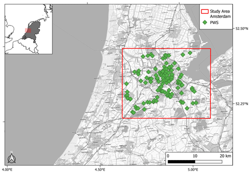
Figure 1 Map of the study area in the Amsterdam metropolitan area in the Netherlands. The red boxes in the map and overview map indicate the domain used for the QC comparison. The PWS locations are denoted by the green diamond symbols. Background map: WMS TopPlusOpen (https://gdk.gdi-de.org/geonetwork/srv/api/records/8BDFB79F-A3FD-4668-88D3-DFD957F265C2, last access: 14 October 2024).

As a reference dataset, a gauge-adjusted radar product from the Royal Netherlands Meteorological Institute (KNMI) with a 1 km spatial resolution and 5 min temporal resolution was used (referred to as the radar reference from here on). It is a climatological product of radar rainfall depths corrected with validated hourly automatic rain gauge measurements and validated daily manual rain gauge measurements, constructed with a considerable delay (i.e. not real-time available), available on the KNMI data platform (KNMI, 2023). Additional details on its construction can be found in Overeem et al. (2009a, b, 2011). It may seem contradictory to consider a radar product as ground truth, while making the case that PWS data may significantly improve these existing rainfall measurement techniques. Note that this radar product combines three types of rainfall information (two radars and two gauge networks, one automatic and one manual) with a significant delay, resulting in it being the best available reference to work with. The benefit of PWSs is their high spatial density and availability in real time. By merging radar data with PWS data, the resulting product combines the best from both techniques (see, for example, Overeem et al. (2024); Nielsen et al. (2024); Overeem et al. (2023)).

The results highlight four distinct 24 h rainfall events, selected to represent different spatio-temporal rainfall characteristics. The events were chosen because the majority of PWSs recorded significant rainfall over an extended duration, making them appropriate for the application of quality control (QC) algorithms.

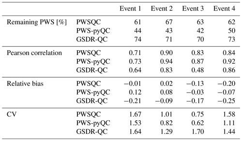
Figure 2 shows the ordinary kriging interpolated rainfall maps on an ∼ 1 km grid after the QC algorithms were applied to the PWS data and the radar reference for event 4 (29 May 2018 08:00–30 May 2018 08:00 UTC). The figures corresponding to the other three events, details on the interpolation method, and the difference maps of the four events can be found in Appendix B. The highest peaks in the radar reference are not captured by PWSQC. The rainfall in the southwest part of the area, where the airport is located and where PWS density is low (see Fig. 1), is underestimated by all, but most severely by GSDR-QC, which is the least sensitive to remove faulty zeroes in the data. PWS-pyQC has the best metrics for this event, although only 50 % of the PWSs are retained on average (see Table E1). The rainfall maps after applying each of the QC algorithms show similar patterns to the radar reference.

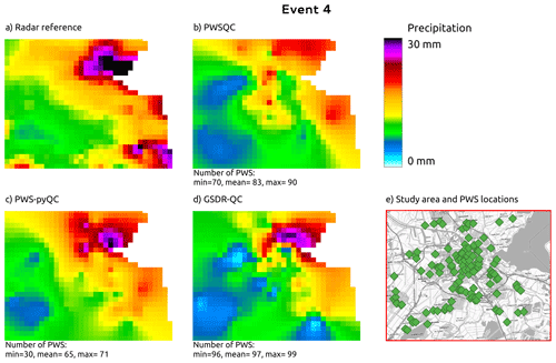
Figure 2 Rainfall maps for event 4. Panel (a) shows the gauge-adjusted radar accumulation. Panels (b), (c), and (d) show the interpolated PWS accumulations using the QC algorithms PWSQC, PWS-pyQC, and GSDR-QC, respectively. Panel (e) shows the locations of all PWSs. Under each map, the data availability after QC is indicated by providing the number of PWSs with hourly data that were used to generate interpolated maps for the hour with the fewest (min) and most (max) PWSs remaining after QC, as well as the average (mean) over the 24 h maps. Background map in panel (e): WMS TopPlusOpen (https://gdk.gdi-de.org/geonetwork/srv/api/records/8BDFB79F-A3FD-4668-88D3-DFD957F265C2).

GSDR-QC shows the most remaining data after QC, while PWS-pyQC rejects most PWSs on average. This is related to the faulty zero checks in the other two methods that are implemented at the sub-daily timescale, whereas GSDR-QC applies the check to daily aggregated data, resulting in reduced sensitivity to missing observations (see also the scatter plots in Appendix C). Hence, because no bias correction is implemented in GSDR-QC, the tendency for a higher negative bias was to be expected. Results after PWS-pyQC yield similar values for bias and Pearson correlation as PWSQC, and values for the coefficient of variation are smaller than the other two QC methods.

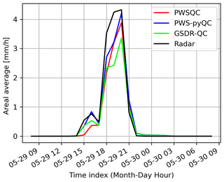
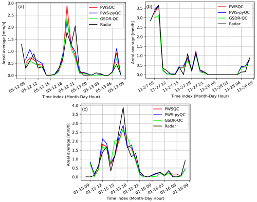
Figure 3 shows an example of the hourly rainfall spatially averaged over the full domain for event 4. The spatially averaged rainfall after all methods were applied approximates the radar reference well, with the least underestimation in PWSQC and PWS-pyQC. Even though the spatial rainfall maps present large differences as seen in Fig. 2, this is largely averaged out over the domain. More results regarding the four events can be found in Appendix C, D, and E. These results provide insight into the number of remaining data, correspondence with radar reference regarding spatial patterns, areal averages, and overall performance metrics for the study area. The relative performance should be interpreted as indicative, as they do not constitute a complete benchmark study.

Figure 3 Example of areal rainfall over the Amsterdam metropolitan area for event 4.

5 Discussion

In this technical note, a guideline to using three different QC algorithms was presented. Interested users have the chance to familiarize themselves with each individual QC and gain insight into their use. The information presented in Table 1 provides a comprehensive overview of the main differences between the three QC algorithms. This information should be beneficial for new users who are interested in using the QC algorithms. For instance, PWSQC does not require any additional information from more reliable observations and can thus be used in areas without reference data, where only PWS data are available. PWS-pyQC requires a reference dataset (primary stations) to derive information about the spatial pattern of indicator correlations and to apply the other filters. Such a dataset can be either a dense rain gauge network or (as shown in this study) a gauge-adjusted radar product. In the absence of such a dataset, PWS-pyQC cannot be used. GSDR-QC requires a reference dataset of gridded precipitation data and user-defined maximum rainfall thresholds. PWS-pyQC typically retains the smallest number of stations compared to PWSQC and GSDR-QC. The indicator correlation filter of PWS-pyQC rejects the complete PWS series, whereas the other QC methods flag and/or remove suspicious individual observations. PWSQC has been applied conservatively: if not enough data are available to determine a flag, the data are not excluded. Given that PWSQC is applicable to 5 min time series and that PWS-pyQC and GSDR-QC are applicable to hourly time series, the calculation of the number of remaining observations is slightly different.

In Table 2, several operational guidelines are provided. Such information is beneficial to select the appropriate QC for the given data availability. The availability of the three QC algorithms within the OpenSense sandbox along with the data from the case study enables testing and experimenting with each QC. Moreover, users can easily modify the QC parameter values without the need to change the main QC functions. Within the case study, the three QC algorithms were applied to the same dataset. An interpolation for one daily event showed that all QC algorithms are able to adequately estimate the average areal rainfall, although the spatial patterns can largely differ. This preliminary analysis cannot provide a detailed comparison between the QC performances. For this, a sensitivity analysis regarding the choice of parameters and reference data would be needed. In addition, long record periods and different climatic conditions would be needed. Such an analysis is beyond the scope of this technical note, as the main aim is to provide interested users with guidelines for using the different QC algorithms. Each QC algorithm was developed and presented in the original studies, where the validity of each QC algorithm was tested (de Vos et al., 2019; Bárdossy et al., 2021; Lewis et al., 2019). The PWS dataset used in this study is of a relatively small size. Upscaling the QC algorithms for larger datasets, e.g. covering Europe (Netatmo , 2021), requires additional steps. For instance, PWS-pyQC applies the filters for every PWS independently; hence, a parallelization of the filters allows for handling large datasets and time-consuming steps. PWSQC cannot be parallelized per time subset due to lead-up time. Parallelization per subset of stations is possible, but the whole PWS dataset needs to be within the working memory of each parallel run to ensure that a PWS's neighbours are always part of the analysis. An alternative approach is used in Overeem et al. (2024) and in the application of spin-off code from Van Andel (2021) on Dutch water board gauge data, to apply the FZ and HI filters only, as these are more efficiently run than the SO filter and bias correction factor allocation. GSDR-QC is easily run in parallel as each rain gauge is analysed in a separate process and as multiple gauges may be analysed simultaneously. The Python code has been written to be efficient, and the whole case study sample is processed in a few minutes on an eight-core laptop. GSDR-QC is therefore the fastest to implement as it was designed for the quality control of a global dataset.

6 Conclusions and outlook

In this work, we presented guidelines for using open-source QC algorithms for PWS rainfall data based on a single dataset and a case study. The aim was to provide an example of how QC for PWSs can be used and to contextualize the additional input data requirements and the technical and operational guidelines for the individual QC methods. Interested users can select the most appropriate QC algorithm for their case study, and whilst the subsequent dataset might not be perfect, there is an improvement from the raw data. Studies like the ones from Bárdossy et al. (2022) and Overeem et al. (2024) have shown the added value of PWSs for improving rainfall estimates for extreme events in Germany and quantitative precipitation estimation on a European scale, respectively.

In our example, all presented QC methods improve the quality of PWS rainfall data; however, this single example does not provide sufficient data to accurately benchmark the three algorithms. Additional work is required for comprehensive sensitivity testing across a range of environments, monitoring networks, and weather patterns to provide more quantitative guidance on the most appropriate QC method.

We make a plea for open-access opportunistic sensing data on a European or even global level (or restricted access for research purposes), which would foster the development and improvement of QC and rainfall-retrieval algorithms. Eventually, this will lead to improved precipitation products and applications such as validation of weather/climate models, hydrological modelling, nowcasting, etc. Furthermore, there is a need for large benchmark radar and rain gauge datasets from different regions and climates. Such benchmark datasets would facilitate a fair intercomparison of QC algorithms and even different opportunistic sensor rainfall estimates from commercial microwave links (CMLs) and satellite microwave links (SMLs). Intercomparison studies also require appropriate metrics and the aforementioned datasets. A discussion on standardized benchmark metrics to be used for intercomparison studies is needed. Benchmarking and intercomparison of algorithms for opportunistic sensor data, merging of opportunistic sensor data and traditional data from rain gauges and radars, and the integration of these data into standard observation systems are objectives that are currently being addressed in the OpenSense COST Action project (https://opensenseaction.eu/).

An ongoing activity within working group 2 of the OpenSense COST Action project is the open-source software implementation the QC algorithms for processing OS data. The aim is to develop a Python module which includes all modules of the QC algorithms presented in this paper. In the long run, this will replace the current QC algorithms in the OpenSense sandbox and will allow users to apply and even combine these in a uniform standardized programming language.

Appendix A: Metrics for all four events

For the four events, 24 h accumulations maps based on hourly interpolations were derived and compared. Subsequently, hourly areal averages over the study domain were calculated and compared. Furthermore, the number of remaining stations was calculated. A point value comparison was done by calculating the pair-wise correlation value, the bias, and the coefficient of variation (CV) between the PWS and reference data for all PWSs locations in the study domain.

The first evaluation metric is the Pearson correlation. It is a widely used pair-wise dependence measure to identify the presence (or absence), the strength, and the direction of a linear relationship between pairs of variables (e.g. x and y). The equation for calculating the Pearson correlation is

$$\begin{array}{}\text{(A1)}& r_{xy}={\displaystyle \frac{{\sum }_{i=\mathrm{1}}^n(x_i-\stackrel{\mathrm{‾}}{x})(y_i-\stackrel{\mathrm{‾}}{y})}{\sqrt{{\sum }_{i=\mathrm{1}}^n(x_i-\stackrel{\mathrm{‾}}{x}{)}^{\mathrm{2}}}\sqrt{{\sum }_{i=\mathrm{1}}^n(y_i-\stackrel{\mathrm{‾}}{y}{)}^{\mathrm{2}}}}}={\displaystyle \frac{\mathrm{cov}(X,Y)}{{\mathit{\sigma }}_X{\mathit{\sigma }}_Y}}.\end{array}$$

The second metric is the relative bias (RB) defined as follows:

$$\begin{array}{}\text{(A2)}& \mathrm{RB}={\displaystyle \frac{\stackrel{\mathrm{‾}}{(x-y)}}{\stackrel{\mathrm{‾}}{y}}}.\end{array}$$

The third metric is the coefficient of variation (CV, Eq. A3) and is used to quantify the dispersion in the data

$$\begin{array}{}\text{(A3)}& \mathrm{CV}={\displaystyle \frac{\mathit{\sigma }(x-y)}{\stackrel{\mathrm{‾}}{y}}},\end{array}$$

where x is the variable to evaluate, y is the reference variable, σ is the standard deviation, r_xy is the Pearson correlation coefficient, x_i is the value of x at time interval i, $\stackrel{\mathrm{‾}}{x}$ is the average value of time series x, y_i is the value of y (the reference) at time interval i, $\stackrel{\mathrm{‾}}{y}$ is the average value of time series y (the reference), and n is the number of observations.

Table A1 Overview of the four rainfall events chosen for this case study.

Appendix B: Additional rainfall maps

Figures B1–B3 show the interpolated 24 h rainfall map after the corresponding QC algorithms were applied. Figures B4–B7 show that the filtered and corrected PWS data are interpolated using ordinary kriging (OK) on the same grid as the reference dataset. OK utilizes the spatial configuration of the points, which is quantified by a fitted variogram model. The latter is derived in the rank space domain following the procedure in Lebrenz and Bárdossy (2017). The parameters (sill and range) were further adapted to adhere with the bounds and order of magnitudes with those derived for the Dutch conditions in the work by Van de Beek et al. (2012). In case no suitable variogram could be derived, e.g., due to the large number of zeros, an average spherical variogram was used, without a nugget value and with a sill scaled according to the data variance. For every hour of the selected daily event with positive PWS observations, the values in the domain are spatially interpolated. The number of accepted PWSs is accordingly noted. The daily map is acquired by accumulating the hourly maps.

For event 2 (Fig. B2), all QC methods show more spatial variability than the radar reference, which is caused by some faulty zeros which are not detected by PWSQC or GSDR. Also, some higher values appear which were obviously not identified as outliers by the QC methods. For event 3 (Fig. B2), there is a very evident outlier PWS with high rainfall amounts over 30 mm. This outlier was not detected by PWSQC and GSDR.

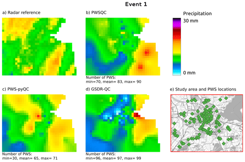
Figure B1 Rainfall maps for event 1. Panel (a) shows the gauge-adjusted radar accumulation. Panels (b), (c), and (d) show the interpolated PWS accumulations using the QC algorithms PWSQC, PWS-pyQC, and GSDR-QC, respectively. Panel (e) shows the locations of all PWSs. Under each map, the data availability after QC is indicated by providing the number of PWSs with hourly data that were used to generate interpolated maps for the hour with the fewest (min) and most (max) PWSs remaining after QC, as well as the average (mean) over the 24 h maps. Background map in panel (e): WMS TopPlusOpen (https://gdk.gdi-de.org/geonetwork/srv/api/records/8BDFB79F-A3FD-4668-88D3-DFD957F265C2).

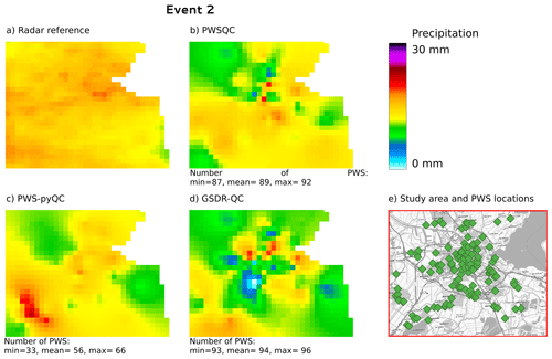
Figure B2 Rainfall maps for event 2. Panel (a) shows the gauge-adjusted radar accumulation. Panels (b), (c), and (d) show the interpolated PWS accumulations using the QC algorithms PWSQC, PWS-pyQC and GSDR-QC, respectively. Panel (e) shows the locations of all PWSs. Under each map, the data availability after QC is indicated by providing the number of PWSs with hourly data that were used to generate interpolated maps for the hour with the fewest (min) and most (max) PWSs remaining after QC, as well as the average (mean) over the 24 h maps. Background map in panel (e): WMS TopPlusOpen (https://gdk.gdi-de.org/geonetwork/srv/api/records/8BDFB79F-A3FD-4668-88D3-DFD957F265C2).

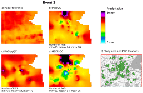
Figure B3 Rainfall maps for event 3. Panel (a) shows the gauge-adjusted radar accumulation. Panels (b), (c), and (d) show the interpolated PWS accumulations using the QC algorithms PWSQC, PWS-pyQC, and GSDR-QC, respectively. Panel (e) shows the locations of all PWSs. Under each map, the data availability after QC is indicated by providing the number of PWSs with hourly data that were used to generate interpolated maps for the hour with the fewest (min) and most (max) PWSs remaining after QC, as well as the average (mean) over the 24 h maps. Background map in panel (e): WMS TopPlusOpen (https://gdk.gdi-de.org/geonetwork/srv/api/records/8BDFB79F-A3FD-4668-88D3-DFD957F265C2).

Figure B4 Differences between the radar reference and the interpolated maps from the three QC algorithms for event 1.

Figure B5 Differences between the radar reference and the interpolated maps from the three QC algorithms for event 2.

Figure B6 Differences between the radar reference and the interpolated maps from the three QC algorithms for event 3.

Figure B7 Differences between the radar reference and the interpolated maps from the three QC algorithms for event 4.

Appendix C: Scatter plots for the four selected events

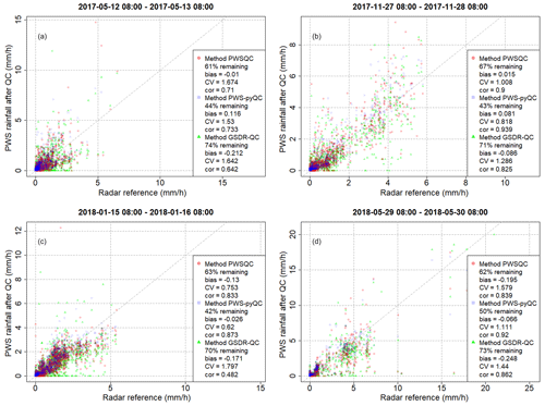
Figure C1 shows four scatter plots for the chosen events. The scatter plots are derived by comparing the hourly PWS data after QC has been applied with a gauge-adjusted radar product, more specifically the overlying pixel of these PWS locations. Only the remaining hourly intervals for every QC method were considered. The data of PWSQC are displayed by the red dots, those of PWS-pyQC are displayed by the blue squares, and those of GSDR-QC are displayed by the green triangles. For every event, several metrics are calculated and showcased within each plot. For each QC method, the number of total data points in the event (134 PWSs × 24 time steps) that is covered after filtering is provided as a percentage. Given that we did not start off with 100 % data availability in the original PWS dataset, this should only be interpreted relative to the other QC method outcomes. This shows that after PWS-pyQC, most data are rejected.

GSDR-QC shows more remaining data after QC; evident are the 0 mm precipitation records in PWS data, while the radar reference records rainfall (the dots spread out horizontally on the x axis). This is due to faulty zero checks in the other two methods being implemented at the sub-daily timescale, whereas GSDR-QC applies the check to daily aggregated data, resulting in reduced sensitivity to missing observations.

Figure C1 The scatter plots of hourly rainfall amounts of PWS after QC is applied against the gauge-adjusted radar reference at the PWS location, including metrics for each of the three QC algorithms. Panels (a) to (d) correspond to the considered events 1 to 4, respectively.

Appendix D: Areal rainfall

Figure D1 Panels (a), (b) and (c) show the areal rainfall over the Amsterdam metropolitan area for events 1, 2, and 3, respectively.

Appendix E: Metrics calculated for the four events

Table E1 Comparison metrics calculated for the four events.