Multi-objective calibration and evaluation of the ORCHIDEE land surface model over France at high resolution

Here we present a strategy to obtain a reliable hydrological simulation over France with the ORCHIDEE land surface model. The model is forced by the SAFRAN atmospheric reanalysis at 8 km resolution and hourly time steps from 1959 to 2020 and by a high-resolution DEM (around 1.3 km in France). Each SAFRAN grid cell is decomposed into a graph of hydrological transfer units (HTUs) based on the higher-resolution DEM to better describe lateral water movements. In particular, it is possible to accurately locate 3507 stations among the 4081 stations collected from the national hydrometric network HydroPortail (filtered to drain an upstream area larger than 64 km²). A simple trial-and-error calibration is conducted by modifying selected parameters of ORCHIDEE to reduce the biases of the simulated water budget compared to the evapotranspiration products (the GLEAM and FLUXCOM datasets) and the HydroPortail observations of river discharge. The simulation that is eventually preferred is extensively assessed with classic goodness-of-fit indicators complemented by trend analysis at 1785 stations (filtered to have records for at least 8 entire years) across France. For example, the median bias of evapotranspiration is −0.5 % against GLEAM (−4.3 % against FLUXCOM), the median bias of river discharge is 6.3 %, and the median Kling–Gupta efficiency (KGE) of square-rooted river discharge is 0.59. These indicators, however, exhibit a large spatial variability, with poor performance in the Alps and the Seine sedimentary basin. The spatial contrasts and temporal trends of river discharge across France are well represented with an accuracy of 76.4 % for the trend sign and an accuracy of 62.7 % for the trend significance. Although it does not yet integrate human impacts on river basins, the selected parameterization of ORCHIDEE offers a reliable historical overview of water resources and a robust configuration for climate change impact analysis at the nationwide scale of France.

1 Introduction

1.1 Land surface models for high-resolution hydrological simulations

Land surface models (LSMs) are the land surface components of Earth system models (ESMs) that simulate water, energy and carbon fluxes across continents. The offline use of LSMs as independent physically based distributed hydrological models has emerged in recent decades for evaluating water resources and investigating climate change impacts at both regional and global scales (e.g., Cai et al., 2014; Pokhrel et al., 2021; Telteu et al., 2021).

Since LSMs provide the lower boundary to atmosphere circulation in ESMs, the spatial discretization of LSMs is usually consistent with the atmospheric component or atmospheric forcing (in offline mode); therefore spatial discontinuity can be averted during land–atmosphere coupling. However, the spatial resolution of the atmosphere component, typically 0.5° (IPCC, 2023), or the atmospheric forcing, typically tens of kilometers (e.g., EuroCORDEX at 11 km in Jacob et al., 2014 and ERA-5 at 31 km in Hersbach et al., 2020), are too coarse to represent topographic details. In addition, river flows are much more constrained by topographic conditions than by the atmosphere. Thus, accurate hydrological simulations for flood risk assessment, drought monitoring and human impact assessment (e.g., dam regulation and irrigation) are difficult to achieve, especially for local-scale implementations. Hence, incorporating high-resolution river routing systems into LSMs is necessary to improve hydrological simulations by better characterizing the morphological conditions of river basins with high-resolution digital elevation models (DEMs) (Bierkens et al., 2015).

The conventional approach to computing river basin discharge levels relies on independent runoff routing models (RRMs) that interpolate the lateral water flows simulated by the LSM to the grid cells of the RRMs and cascade river discharge levels along the drainage network. The RRMs represent the horizontal movements of water fluxes, while their vertical movements are kept in LSMs. There are many different RRMs in the literature, such as the TRIP at 0.5° resolution (Oki and Sud, 1998; Oki et al., 1999; Vergnes and Decharme, 2012), the RiTHM at 0.25° resolution (Ducharne et al., 2003) and the HYDRA at 5^′ resolution (Coe, 2000). To bridge the gap between high-resolution hydrological simulations and coarse LSM grid cells, the concept of constructing hydrological transfer units (HTUs) in LSM grid cells with high-resolution DEMs was proposed to better represent natural river systems (Nguyen-Quang et al., 2018; Polcher et al., 2023). These hydrologically consistent units within each atmospheric grid cell are connected to horizontally transfer the simulated lateral flows; therefore the generated river flows in one atmospheric grid cell can flow into neighboring grid cells (HTU to HTU and then grid cell to grid cell) (Polcher et al., 2023). The vertical and horizontal movements of water fluxes can be maintained within the LSM instead of separating these two movements by two models (i.e., LSMs and RRMs) at different resolutions, which facilitates the representation of human impacts on hydrological processes (Zhou et al., 2021; Baratgin et al., 2024).

1.2 How are land surface models calibrated?

When using LSMs to simulate realistic water fluxes, including river discharge, a calibration step is often necessary: even if LSMs are designed to be as physical as possible, they inevitably contain parameters that are hard to measure directly, such as vegetation water stress (Ruiz-Vásquez et al., 2023) or soil properties at different depths (Yang et al., 2016). Traditional hydrologic calibration is primarily conducted against river discharge observations (e.g., Troy et al., 2008; Gou et al., 2020; Cho and Kim, 2022; Rummler et al., 2022), which is considered to be a well-suited benchmark (Prentice et al., 2015). However, calibrating physically based LSMs to discharge alone does not guarantee the realistic representation of hydrological processes and the accurate simulation of other LSM outputs, such as soil moisture (Sutanudjaja et al., 2014) and evapotranspiration (Rajib et al., 2018a, b). Over recent decades, the advancement of reanalysis and remote-sensing data quality at fine scales, such as snow cover (Hall et al., 2002), evapotranspiration (Martens et al., 2017) and soil moisture (Dorigo et al., 2017) products, provides new opportunities to investigate and improve the effectiveness of LSMs in representing water fluxes. Multi-objective calibration works that combine discharge observations with these data products have shown an overall improvement in hydrological simulation performance (e.g., López López et al., 2017; Jiang et al., 2020; Yang et al., 2021).

The complexity of LSMs makes their calibration extremely difficult in practice because their large number of parameters induces high degrees of freedom (Fisher and Koven, 2020). Two kinds of methods are mostly used to adjust the parameter set of LSMs: automatic (i.e., optimization techniques) and manual (i.e., trial-and-error procedure). Numerous efforts have been put into optimization algorithms (e.g., Müller et al., 2015; Yang et al., 2021; Cheng et al., 2023), with the major challenge being the computational burden, especially for high-resolution applications (Bierkens et al., 2015; Sun et al., 2020). Another limitation of the automatic calibration method, especially if applied to large parameter sets, stems from the equifinality issue that many different parameter sets lead to equally good results (Beven, 2006; Fisher and Koven, 2020). In manual calibration practice, modelers select a few parameter sets, apply them to run the LSM, and choose the best parameter set based on evaluations. Albeit highly dependent on expert judgment, this method can be efficient in saving model run time compared to the hundreds of model runs required by automatic methods (Schaperow et al., 2021). Either way, a perfect calibration is always impossible to achieve due to inherent uncertainties in forcing data (e.g., Gelati et al., 2018; Kabir et al., 2022), benchmark observations (e.g., Zeng and Cai, 2018) and model structure (e.g., van Kempen et al., 2021).

1.3 How is the performance of land surface models evaluated?

Hydrological model performance is typically evaluated with goodness-of-fit indicators, such as Kling–Gupta (Kling et al., 2012) or Nash–Sutcliffe (Nash and Sutcliffe, 1970) efficiencies. In doing so, discharge is often transformed for performance evaluation, such as with logarithms for the emphasis of low flows (Santos et al., 2018) or with square roots to balance low and high flows (Song et al., 2019). Hydrological signatures that characterize statistical or dynamic features of discharge (e.g., annual discharge and low flow duration) can also be used to evaluate simulation performance (see the review by McMillan, 2021). These traditional indicators implicitly assume stationary conditions and are no longer sufficient since “stationarity is dead” (Milly et al., 2008). As shown by Todorović et al. (2022), the traditional indicators do not guarantee the reproduction of streamflow trends with hydrological models. Thus, trend analyses are important to evaluate the robustness of hydrological models in the long term, which is essential to subsequent applications for climate change assessment (Fowler et al., 2020).

1.4 Aim and novelty of the study

At the nationwide scale of France, the first distributed LSM for hydrological applications was proposed by Habets et al. (2008). It couples the SAFRAN atmospheric reanalysis system (Vidal et al., 2010a) and the ISBA LSM (Decharme and Douville, 2006), both at a spatial resolution of 8 km × 8 km, and the MODCOU model (Ledoux et al., 1989) for groundwater and river flow, with a variable resolution down to 1 km along rivers. This model, called SIM, short for SAFRAN–ISBA–MODCOU, was validated by comparison to hundreds of hydrometric stations with a focus on the Seine, Loire, Garonne, and Rhône River basins, the four major river basins in France from 1995 to 2005. Observations of piezometric head and snow depth at several sites are also used to evaluate the SIM model. Since then, it has been used to assess drought risks in the atmosphere, soils and rivers and to investigate the impact of climate change for future adaptation at the national scale (e.g., Quintana Seguí et al., 2009; Vidal et al., 2010b; Boé et al., 2009) and recently improved to better describe the water and energy budgets in France from 1958 to 2018, providing an extensive historical analysis (Le Moigne et al., 2020).

The main goal of the present study is to obtain a reliable and robust hydrological simulation over France with another LSM, the Organising Carbon and Hydrology in Dynamic Ecosystems (ORCHIDEE) LSM, using a high-resolution HTU-based routing scheme (Nguyen-Quang et al., 2018; Polcher et al., 2023). This approach allowed us to simulate river discharge at thousands of hydrometric stations across French rivers, supporting a thorough performance evaluation. In doing so, we combined traditional indicators implicitly assuming stationary conditions and indicators about trend accuracy because “stationarity is dead” (Milly et al., 2008). Another novelty stems from a multi-objective calibration focused on the water budget, benefiting from river discharge observations at 1785 hydrometric stations and evapotranspiration products. The parameterization selected in this study has been used to project the impact of climate change on French water resources, which contributes to the national Explore2 project (https://professionnels.ofb.fr/fr/node/1244, last access: August 2024) for future adaptation design. Here, we only present the simulation results from 1959 to 2020 to assess the performance of the ORCHIDEE LSM. In Sect. 2, the ORCHIDEE LSM is presented, followed by a summary of the input data, the benchmark datasets, and the calibration strategy. In Sect. 3, we detail the calibration procedure that was conducted step by step to improve the overall simulated water budget and evaluate the simulation which was eventually chosen with classic goodness-of-fit measures and trend analysis; finally, a discussion and conclusions are presented.

2 Materials

2.1 The ORCHIDEE LSM

The ORCHIDEE model is a physically based LSM developed at the Institut Pierre Simon Laplace (IPSL) as the land component of the IPSL climate model, which is used for all the past and future climate simulation exercises carried out for the IPCC reports as part of the Coupled Model Intercomparison Project (CMIP) (IPCC, 2023). Here, we use ORCHIDEE version 2.2 (with revision 7738), which is very close to the version used as the land component of the IPSL-CM6 climate model (Boucher et al., 2020; Cheruy et al., 2020). In this study, the ORCHIDEE model is not coupled to the IPSL climate model (offline simulation) but is instead fed by an atmospheric forcing (Sect. 2.2.1). The ORCHIDEE model couples the SECHIBA (water and energy budgets in Ducoudré et al., 1993) and STOMATE (carbon budget and phenology in Krinner et al., 2005) modules. This coupling describes the hydrological processes (e.g., soil moisture diffusion, evapotranspiration and river discharge) and their interactions with vegetation and the carbon cycle; therefore the simulated variables depend on the atmospheric CO₂ concentration. The water, energy and carbon fluxes are calculated on a 30 min time step within each atmospheric grid cell, and the river discharge levels are then deduced by aggregating the lateral flows of each grid cell along the river routing network. It must be noted that this version of ORCHIDEE does not include any human impact, with the exception of the presence of crops among the possible vegetation types.

The vegetation in a grid cell is not uniform but rather comprises a mosaic of several plant function types (PFTs; Sect. 2.2.2). Table S1 in the Supplement summarizes the 15 PFTs used in the ORCHIDEE LSM. Each PFT is characterized by different morphological, physiological, phenological and radiative properties, mainly based on the specialized literature. The root density profile of each PFT in the ORCHIDEE model is assumed to decrease exponentially with depth and is modulated by a decay factor c, as shown in Fig. S9. The root density of each PFT can be increased (decreased) by decreasing (increasing) c. Crop and grass PFTs have higher c values than forest PFTs; the roots of crop and grass PFTs are concentrated in surface soil layers, while the roots of forest PFTs can pass through deep soil layers.

The soil is 2 m deep, and each grid cell is characterized by the dominant soil texture (Sect. 2.2.2). The soil water retention properties (including porosity θ_s, field capacity θ_c and wilting point θ_w) depend on the texture as detailed in Table S2. The soil hydraulic conductivity at saturation K_s is not vertically constant, as shown in Fig. S5: ORCHIDEE assumes an exponential decrease with depth due to soil compaction, ruled by a decay factor f, combined with an increase towards the soil surface due to the presence of roots, which enhances infiltration capacity (de Rosnay et al., 2002; d'Orgeval et al., 2008). This effect depends on the root density profile. At each time step, soil moisture is redistributed vertically according to the Richards equation (flow in an unsaturated medium), taking into account surface boundary conditions by infiltration and soil evaporation, withdrawals by roots through the entire soil depth to supply transpiration, and gravitational drainage at the bottom of the soil (Campoy et al., 2013; Tafasca et al., 2020). For accurate computation, soil moisture and vertical water fluxes are discretized across 22 layers over 2 m, with 7 soil layers of increasing depth in the top 20 cm to capture the strong soil moisture gradients and then soil layers of constant thickness (12.5 cm) down to the soil bottom (Campoy et al., 2013). In this framework, transpiration depends on soil moisture and a factor p, which represents the soil moisture content above which transpiration is maximal, i.e., not limited by water stress. Figure S7 shows how the parameter p constrains transpiration.

Evapotranspiration (ET) is calculated as the sum of plant transpiration, evaporation of intercepted water, soil evaporation and snow sublimation. This calculation does not depend on potential evapotranspiration, but it is coupled to the surface energy balance, which requires a sub-hourly time step (here 30 min) to describe the diurnal radiation cycle. The four ET fluxes in ORCHIDEE are described by a bulk aerodynamic formulation, in which the roughness length for momentum z_0m and for heat z_0h controls the aerodynamic resistance. z_0m and z_0h in ORCHIDEE can be calculated by prescribed parameters: z_0m is calculated by a first-order approximation of vegetation height, i.e., multiplied by a factor f_z (e.g., $\mathrm{1}/\mathrm{10}$ in Brutsaert, 2005), and $z_{\mathrm{0}\mathrm{m}}/z_{\mathrm{0}\mathrm{h}}$ is parameterized as 1 in CMIP5 to compensate for forcing errors (Dufresne et al., 2013). Note that $z_{\mathrm{0}\mathrm{m}}/z_{\mathrm{0}\mathrm{h}}$ should be larger than 1; for example, $z_{\mathrm{0}\mathrm{m}}/z_{\mathrm{0}\mathrm{h}}=\mathrm{10}$ was proposed by Brutsaert (2005). z_0m and z_0h in the ORCHIDEE can also be calculated as a function of leaf area index (LAI) by the dynamic (dyn) method proposed by Su et al. (2001), as implemented in CMIP6 (Boucher et al., 2020). The formulation of the method as well as its application is detailed in Su et al. (2001) and Su (2002). This dynamic method generally decreases ET simulation for the CMIP6 configuration of ORCHIDEE compared with the CMIP5 configuration.

Snowpack and its dynamics are described by a three-layer model, which makes it possible to account for variations in albedo, density and thus the insulating properties of the snowpack as a function of the age of the snow and the nature of the underlying vegetation (Wang et al., 2013). Rainfall not intercepted by vegetation cover and meltwater can infiltrate or become runoff when the rainfall exceeds the surface hydraulic conductivity. The two runoff terms, surface runoff and gravitational drainage at the bottom of the soil, are summed as the total runoff.

Eventually, river flows are calculated by a high-resolution routing model (Nguyen-Quang et al., 2018; Polcher et al., 2023), which aggregates the total runoff of HTUs within each atmospheric grid cell along the river routing network (Sect. 2.2.3). The routing model contains three linear reservoirs in each HTU: the river reservoir allows horizontal flow to transfer from HTU to HTU along the high-resolution river network; the groundwater and surface water reservoirs are used to compute the mean transit time of groundwater drainage and surface runoff, respectively, and their contribution to the outflow from the river reservoir (Schrapffer et al., 2020). The groundwater reservoir is simplified as a free aquifer, and thus the outflow is the base flow. The resident time of each reservoir depends on the length and slope of the HTU, modulated by a time constant specific to each reservoir (Polcher et al., 2023), which leads to a duration of resident time from long to short according to the order of groundwater, surface water and river reservoirs. In this context, the flow velocity in each HTU in the river reservoir does not vary with discharge and does not depend on flooding, which is not explicitly described.

2.2 Input data over France

2.2.1 Atmospheric forcing

The near-surface meteorological SAFRAN reanalysis with a spatial resolution of 8 km and a temporal resolution of hourly time steps (Vidal et al., 2010a) is used in this study to drive the ORCHIDEE simulations over France. The SAFRAN grid cell is thus the horizontal resolution of the ORCHIDEE simulations. To cover the complete drainage area of French rivers, especially in the eastern Alpine parts of France, the SAFRAN reanalysis was extended to some parts of neighboring countries, especially Switzerland (Fig. 1). The SAFRAN reanalysis is available from August 1958 onwards and contains atmospheric data for ORCHIDEE: air temperature, air pressure, air specific humidity, wind speed, liquid and solid precipitation, and downwards longwave and shortwave radiation. In addition, annual CO₂ concentration observations in the atmosphere are sourced from Lurton et al. (2020).

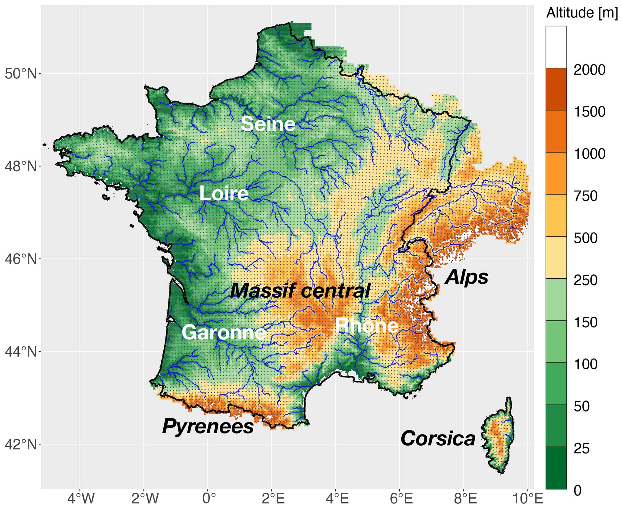
Figure 1 The topography and hydrography of Metropolitan France (including Corsica), delineated in black contours, extended to neighboring countries based on the upscaled MERIT Hydro DEM. The river networks in blue are represented by the pixels with a flow accumulation larger than 200 pixels. Four major river basins, the Seine, the Loire, the Rhône and the Garonne, and three major mountain ranges, the Alps, the Massif Central and the Pyrenees, in France are marked on the map. The gray points represent the central points of the SAFRAN reanalysis grid cells.

2.2.2 Boundary conditions: soil, vegetation and land use

The annual vegetation and land use maps for France used in this study are sourced from Lurton et al. (2020) and derived from two products (see https://orchidas.lsce.ipsl.fr/dev/lccci/, last access: August 2024, for further data aggregation information): the global ESA CCI vegetation distribution (Harper et al., 2023) at 300 m spatial resolution is used to generate 15 generic PFTs gridded at 0.25° spatial resolution for the ORCHIDEE model (bare soil, 2 crop PFTs, 4 grass PFTs and 8 forest PFTs as detailed in Table S1) to represent land cover distribution; the distribution of the 15 generic PFTs is then combined with the Land-Use Harmonization 2 (LUH2) dataset (Hurtt et al., 2020) at 0.25° spatial resolution to produce the temporal evolution of 15 PFTs for CMIP6 simulations over the historical and future periods (850–2100). This information is ultimately reaggregated into SAFRAN grid cells to account for the spatial distribution of the PFTs across France (Fig. S1 in the Supplement). The harvested wood biomass is also sourced from the LUH2 dataset.

The sensitivity of the ORCHIDEE model to global and regional soil texture maps was tested in the literature (e.g., Tafasca et al., 2020; Kilic et al., 2023). The global soil texture map of Reynolds et al. (2000) shows a better hydrological performance for the Seine River basin (Kilic et al., 2023). Therefore, the soil texture data for France used in this study are based on the global soil texture map of Reynolds et al. (2000) at a $\mathrm{1}/\mathrm{12}$° spatial resolution, which classifies soil textures into 12 USDA types. The soil texture information over France is then rescaled into SAFRAN grid cells by keeping the dominant soil texture type for each grid cell (Fig. S2). The dominant soil textures in France are loam and clay loam according to the Reynolds soil texture map.

2.2.3 River routing network

The construction of the river routing network across France for the ORCHIDEE model is based on the DEM at $\mathrm{1}/\mathrm{60}$° resolution (approximately 1.3 km over France), built by upscaling the MERIT Hydro global hydrography map at 3 arcsec resolution (Yamazaki et al., 2019) with the Iterative Hydrography Upscaling (IHU) method (Eilander et al., 2021). The DEM incorporates the following topographic and hydrologic information from the MERIT Hydro dataset: elevation, flow direction, flow accumulation and distance to the ocean for each pixel, as shown in Fig. 1; this information is used to construct the river routing network connected by the HTUs of SAFRAN grid cells as detailed in Polcher et al. (2023). In this study, we selected 15 truncations to construct HTUs (nbmax = 15, i.e., the maximum number of HTUs within each atmospheric grid cell) given the spatial resolutions of the DEM and SAFRAN. Within this framework, the hydrometric stations collected from the Explore2 project are positioned on the constructed high-resolution river routing network to comply with the following criteria: the distance between the real station and the modeled station must be less than 5 km, and the error of the upstream surface at the modeled station must be less than 20 %. Of the 4081 hydrometric stations collected, 3507 stations are within the above tolerance level (86 % of the total stations). Finally, ORCHIDEE can monitor the flow out of the HTU associated with the station during the simulation.

2.3 Evaluation strategy

2.3.1 Evaluation datasets

Three evaluation datasets are used in this study to assess the performance of the ORCHIDEE simulation.

The GLEAM dataset (Martens et al., 2017) provides daily ET data at a 0.25° resolution at the global scale from 1980 to 2020; these data were derived from the Priestley and Taylor (1972) evaporation model with satellite-based products (net radiation, precipitation, surface soil moisture, skin and air temperatures, vegetation optical depth and snow water equivalent) as inputs. The FLUXCOM dataset (Jung et al., 2019) provides daily ET at a 0.5° resolution from 2001 to 2015 based on machine learning algorithms that merge global FLUXNET measurements with remote-sensing and meteorological observations. Both ET benchmarks are aggregated to SAFRAN grid cells at monthly time steps. GLEAM and FLUXCOM provide independent ET estimates, both of them with large uncertainties (Liu et al., 2023). They are used in combination to approach the plausible range of observed ET.

The Explore2 project provides records of daily river discharge (Q) across France extracted from the French national hydrometric HydroPortail (Leleu et al., 2014; Delaigue et al., 2020). Of the 3507 hydrometric stations placed across the constructed river routing network, 1785 stations have Q records for at least 8 entire years over the simulation period of 1959–2020; these records were used to calibrate and evaluate the ORCHIDEE simulation. Stations with Q records for at least 8 entire years were chosen because (1) the simulation performance was shown to be rather insensitive to the length of evaluation period above 8 years (Sect. S10), and (2) these stations offer a large coverage of French rivers.

Although the version of ORCHIDEE used in this study does not include any human impact, the 1785 selected hydrometric stations were all used in the evaluation process, whether human influenced or not. This enables a more comprehensive assessment of ORCHIDEE, as natural or weakly influenced stations are few in number (only 536; see Sect. S9) and exclude the stations along the main streams of the four major French rivers (Seine, Loire, Garonne, and Rhône).

2.3.2 Performance criteria

The criteria bias, Pearson correlation, Kling–Gupta efficiency (KGE; Kling et al., 2012) and time lag are used to quantitatively evaluate the goodness of fit of the simulated ET (at grid cell level over France) and Q against the above datasets. The square-root transformation of Q is applied when calculating the KGE criterion to capture both high and low flows (Song et al., 2019). The time lag calculation is based on auto-correlation with various lags and determined by the lag t giving the maximum correlation (a positive t means that the simulated Q time series lags the observed time series by t days; a negative t means that the simulated Q time series leads the observed time series by −t days). The ideal time lag value is 0.

In addition, to verify the ability of the ORCHIDEE LSM to reproduce the observed trends of ET (at station level as the spatial averages of grid cells in the basins upstream the stations) and Q, the trends of the 1785 selected stations were calculated using Sen's slope estimator (Sen, 1968). The nonparametric Mann–Kendall test (Mann, 1945; Kendall, 1948) was used to determine the significance of the calculated trends. The significance level in this study is set to 5 %. Split sample tests were also performed and showed stable performances if the Q time series are split in two halves (Sect. S11).

We used a confusion matrix and associated metrics to summarize the trend results: the “accuracy” indicates the proportion of correct simulations among all observations, the “PPV” (positive predictive value) and “NPV” (negative predictive value) indicate how many positive/negative simulations are actually correct, and the “TPR” (true positive rate) and “TNR” (true negative rate) indicate how many positive/negative observations are correctly represented by the model. How these classic metrics are calculated is detailed in Ting (2010). In addition, to focus on the accuracy of the simulated trend significance, two metrics “PTSA” (positive trend significance accuracy) and “NTSA” (negative trend significance accuracy) are used to indicate the proportions of accurate trend significance (either significant or not) among all the accurate positive or negative trends. Stations with accurate trend sign but incorrect significance are considered inaccurate in this framework.

2.4 Calibration design

LSMs are complex models, integrating many coupled processes related to hydrology, soils and vegetation but also to the radiative transfer of the boundary layer. They are also distributed models designed to be applied over wide and contrasted domains (Clark et al., 2015), in which every grid point could be regarded as one 1D model. Therefore, their calibration is challenging, and a full optimization of LSM's parameters is practically intractable, due to the computational burden (Bierkens et al., 2015), the equifinality (Fisher and Koven, 2020), and the uncertainty of input and benchmark datasets (Best et al., 2015). The most common solutions are to rely on transfer functions to derive the spatial variations of model parameters from maps of physical parameters (e.g. Samaniego et al., 2010) and to accept sub-optimal but satisfactory performance (Best et al., 2015).

In this line, here we chose to calibrate selected parameters of the ORCHIDEE LSM based on an iterative trial-and-error procedure to gradually improve simulations by manually adjusting some parameters. The simulation period is from 1959 to 2020, with a warm-up from 1959 to 1968 to provide reasonable initial conditions, and the output variables (e.g., ET and Q) are aggregated to daily time steps. The starting experiment of this calibration procedure is called STD and uses the “standard” parameter set sourced from CMIP6 (Boucher et al., 2020), according to which the roughness heights z_0m and z_0h are calculated by the dynamic method of Su et al. (2001). STD forced with SAFRAN reanalysis significantly underestimates ET and overestimates Q compared with the evaluation datasets detailed in Sect. 2.3. The calibration is therefore aimed at increasing ET and decreasing Q. According to expert knowledge on the parameter sensitivity of ORCHIDEE and previous calibration exercises (Kilic et al., 2023; Raoult et al., 2021; MacBean et al., 2020; Dantec-Nédélec et al., 2017; Campoy et al., 2013), we focused on parameters that control surface roughness, soil hydraulics and vegetation morphology (detailed in Sect. 2.1) to improve the simulations of ET and Q.

Table 1 Parameter sets applied to the calibration experiments of the ORCHIDEE LSM. The means of daily evapotranspiration (ET), surface runoff (R_s), drainage (R_d) and total runoff (R) are calculated over the extended SAFRAN coverage and the 1959–2020 simulation period. The medians of ET bias are calculated for all SAFRAN grid cells of the extended SAFRAN coverage with the GLEAM dataset over the 1980–2020 period and with the FLUXCOM dataset over the 2001–2015 period. The median of river discharge (Q) bias is calculated with the 1785 selected French hydrometric stations over the 1959–2020 period.

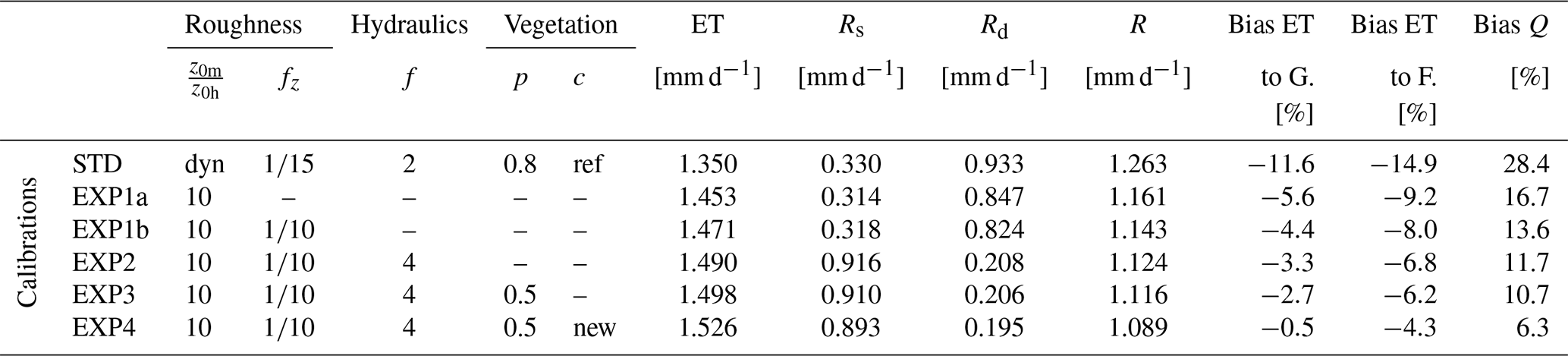
– Same as STD; dyn, dynamic; G., GLEAM; F., FLUXCOM; ref = [5.0, 0.8, 0.8, 1.0, 0.8, 0.8, 1.0, 1.0, 0.8, 4.0, 4.0, 4.0, 4.0, 4.0, 4.0] in Table S1; new = [5.0, 0.8, 0.8, 1.0, 0.8, 1.5, 2.0, 2.0, 1.5, 4.0, 4.0, 2.0, 2.0, 4.0, 6.0] in Table S1.

A hundred parameter sets were tested in this iterative evaluation process, summarized in Table 1 by a selection of six calibration experiments that show a gradual decrease in ET and Q biases on average over France. Each parameter set in Table 1 is applied uniformly over the entire simulation area. EXP1a and EXP1b calculate ET using the prescribed $z_{\mathrm{0}\mathrm{m}}/z_{\mathrm{0}\mathrm{h}}$ and f_z, respectively, with values suggested by Brutsaert (2005). EXP2 increases the decay factor f, and the soil hydraulic conductivity decreases more rapidly with depth; therefore the soil drainage decreases (Q decreases), and ET increases. EXP3 decreases the soil water threshold for transpiration from 0.8 to 0.5, and transpiration (and thus ET) increases. EXP4 changes the root profiles of the PFTs present in France by increasing the c parameter of tree and boreal grass PFTs to decrease their root density, while decreasing the c parameter of crop PFTs to increase crop root density. As such, the transpiration of trees and boreal grasses decreases, while the transpiration of crops increases.

3 Results

3.1 Evaluation of simulated basin area

Figure 2 shows the good performance of the high-resolution river routing model in simulating the basin areas across France, with R²=0.999 across the 3507 stations compared to the information from HydroPortail. Classically, the performance increases with increasing river basin area, with R² ranging from 0.992 for basins less than 10³ km² to 0.998 for basins larger than 10⁴ km². However, the routing model tends to overestimate basin areas for basins less than 10⁴ km² but tends to slightly underestimate basin areas for basins larger than 10⁴ km². There is no significant positive or negative bias in the simulated basin area for the four major river basins (the Seine, the Loire, the Rhône and the Garonne), and the biases of most of the simulated basins are less than 5 %. For basins larger than 10³ km², most of the biases that are larger than 5 % are located in the mountainous regions, especially in the Alps, given the complicated topography.

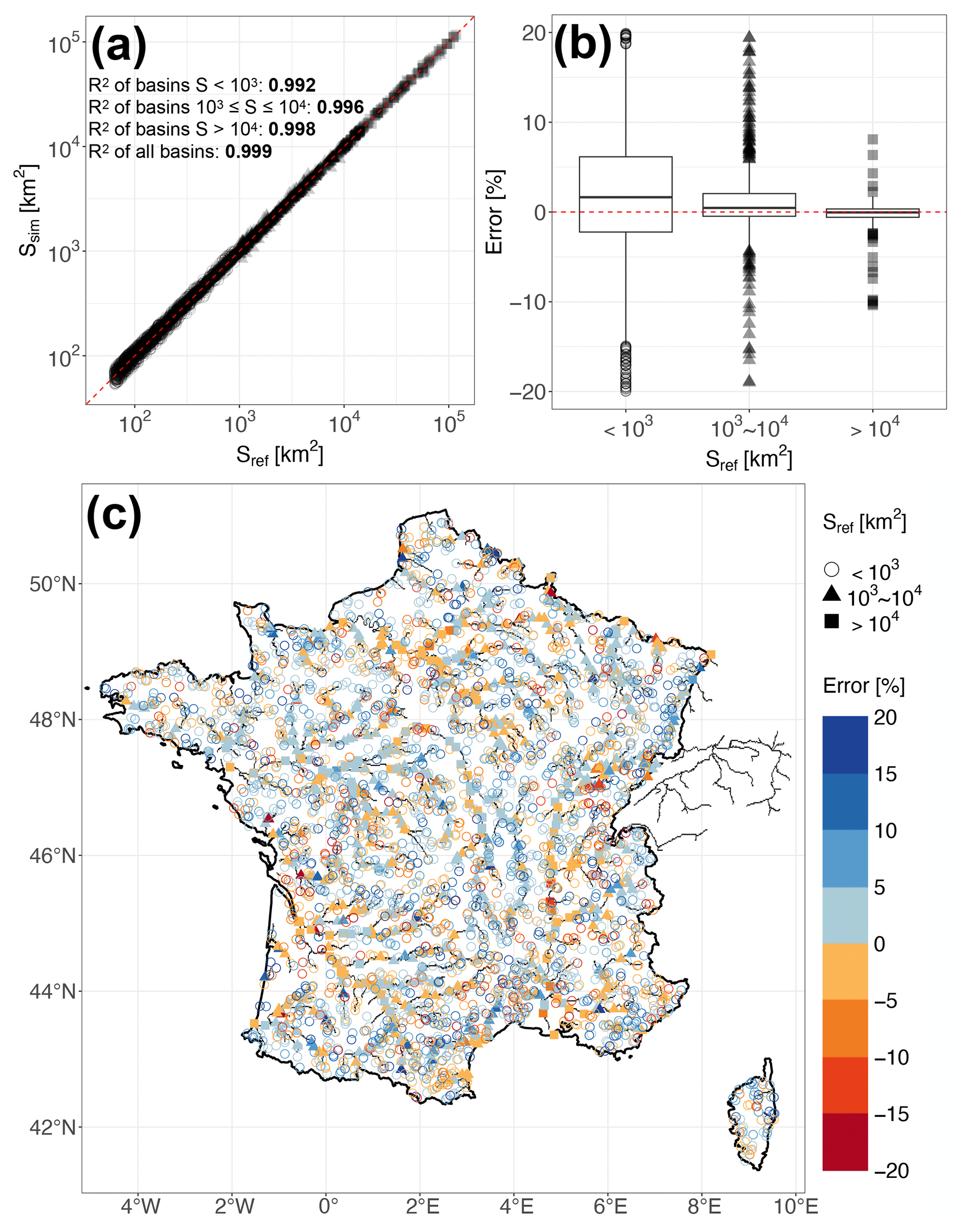
Figure 2 The comparison between the simulated upstream basin area and the reference area in HydroPortail for the 3507 stations located in the high-resolution river networks: (a) scatter plot of simulated area to reference area; (b) box plot of simulated area bias; and (c) spatial map of simulated area bias for basins less than 10³ km², between 10³ and 10⁴ km², and larger than 10⁴ km².

3.2 Performance of the different experiments

Figure 3 illustrates how the performance criteria of the simulated ET and Q improve during the calibration experiments. The first three calibration experiments show the impact of two different methods on calculating ET. STD applies a dynamic physically based model that calculates z_0m and z_0h with the variables simulated by ORCHIDEE (e.g., canopy height, LAI, and fractional coverage for 15 PFTs). EXP1a and EXP1b prescribe $\frac{z_{\mathrm{0}\mathrm{m}}}{z_{\mathrm{0}\mathrm{h}}}$ and f_z values to approximate z_0m and z_0h only with the simulated variable of canopy height. Compared with STD, EXP1a decreases the negative ET bias against FLUXCOM by 5.7 % by greatly increasing z_0h from $\mathrm{1.10}\times {\mathrm{10}}^{-\mathrm{4}}$ to $\mathrm{1.43}\times {\mathrm{10}}^{-\mathrm{2}}$ m over the extended simulation domain and simulation period (z_0m decreases from 0.385 to 0.255 m). Compared with EXP1a, EXP1b decreases the negative ET bias by 1.2 % by increasing f_z from $\mathrm{1}/\mathrm{15}$ to $\mathrm{1}/\mathrm{10}$: z_0m increases from 0.255 to 0.482 m, and z_0h increases from $\mathrm{1.43}\times {\mathrm{10}}^{-\mathrm{2}}$ to $\mathrm{2.28}\times {\mathrm{10}}^{-\mathrm{2}}$ m. Figures S3 and  4 show the spatial and temporal changes of the z_0h, z_0m and ET values for the first three calibration experiments. Q is thus decreased due to the water budget of ORCHIDEE when ET is increased, and the positive Q bias against HydroPortail decreases by 11.7 % and 3.1 %, respectively. For the first three calibration experiments, the biases of simulated ET and Q against observation datasets are gradually decreased, and EXP1a decreases the biases of the simulated ET and Q the most. In addition, the KGE values of square-rooted Q against observations are slightly increased. However, the correlation values of the simulated Q against observations are slightly decreased, and the simulated Q tends to gradually lag behind the observations for the first three calibrations.

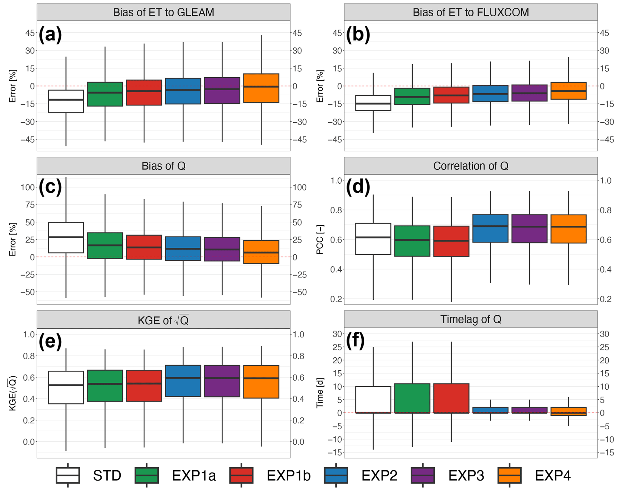
Figure 3 Performance criteria of calibration experiments: (a) bias of the simulated ET to the GLEAM dataset, (b) bias of the simulated ET to the FLUXCOM dataset, (c) bias of the simulated Q, (d) Pearson correlation coefficient of the simulated Q, (e) KGE of the square-rooted simulated Q and (f) time lag of the simulated Q. The calculation of biases for the simulated ET is applied to all SAFRAN grid cells of the extended domain over the 1980–2020 period against the GLEAM dataset and over the 2001–2015 period against the FLUXCOM dataset, respectively. The calculation of criteria for the simulated Q is applied to the 1785 hydrometric stations in the HydroPortail dataset with records for at least 8 entire years. For each box plot, the lower and upper hinges are the first and third quartiles; the minimum and maximum values extend from the first and third hinge to 1.5 times of the interquartile range.

To improve the goodness of fit of the simulated Q, EXP2 increases the decay factor f from 2 to 4 compared to EXP1b, which decreases the hydraulic conductivity for soil layers below 0.3 m, while the hydraulic conductivity for soil layers above 0.3 m remains unchanged (Fig. S6a and b). A decrease in hydraulic conductivity in deep soil layers leads to a decrease in drainage at the soil bottom. Since less water drains from deep soil layers, while the surface soil layers maintain the same infiltration capacity, the latter can saturate more easily, and more surface runoff is produced (Table 1). Eventually, the total runoff is decreased from EXP1b to EXP2 as the surface runoff increase is smaller than the decrease in gravitational drainage at the soil bottom. EXP2 thus decreases the positive Q bias against HydroPortail (by 1.9 %), as well as the negative ET bias against FLUXCOM (by 1.2 %). In addition, the ratio of surface runoff to total runoff is greatly increased from 27.9 % in EXP1b to 81.5 % in EXP2, which results in more “fast” surface flow and less “slow” groundwater, leading to more responsive Q to precipitation events. The correlation and KGE criteria of the simulated Q are improved from 0.59 to 0.69 and from 0.54 to 0.59, respectively (Fig. 3). The time lag criterion of the simulated Q is also greatly improved from a range of −11 to 27 d to a range of −3 to 5 d. Similar improvements in streamflow dynamics could be obtained by changing the time constant of the fast and slow routing reservoirs without improving the Q and ET biases.

Two additional simulations, EXP3 and EXP4, were conducted to further improve the bias criteria by changing the vegetation parameters in ORCHIDEE to potentially increase transpiration (thus ET): EXP3 reduced the soil moisture stress for transpiration, while EXP4 changed the vegetation root profile. Transpiration is conveyed by the factor Us in ORCHIDEE, which is negatively related to the water stress factor F and positively related to root density.

The factor F depends on soil moisture and on a threshold parameter p, as illustrated in Fig. S7: there is no soil moisture stress if F=1, which occurs when the soil moisture exceeds ${\mathit{\theta }}_{\mathrm{w}}+p\times ({\mathit{\theta }}_{\mathrm{c}}-{\mathit{\theta }}_{\mathrm{w}})$. By decreasing p from 0.8 in EXP2 to 0.5 in EXP3, a wider range of soil moisture leads to F=1 and thus unstressed transpiration. As shown in Fig. S8, transpiration (Us) is increased for all PFTs, and the effect is more pronounced for crop PFTs (PFTs 12 and 13) than for forest PFTs (PFTs 7 and 8). However, this general decrease in soil water stress to favor transpiration is weak, as it decreases the negative ET bias against FLUXCOM by only 0.6 % (1.0 % for the positive Q bias against HydroPortail).

The change in the root density profile from EXP3 to EXP4 further modifies transpiration but also changes the hydraulic conductivity of the shallow soil layers. In EXP4, we increased the root density of the crop PFTs (PFTs 12 and 13) by decreasing c and decreased the root density of the forest and boreal grass PFTs (PFTs 6, 7, 8, 9 and 15) by increasing c (Table S1; Fig. S9). Given the major spatial distribution of the crop PFTs in France (Fig. S1 in the Supplement), the general effect of EXP4 compared to EXP3 increases transpiration (thus ET), which also reduces drainage at the soil bottom. In addition, the hydraulic conductivity of the shallow soil layers in France is slightly increased but with some spatial differences, as shown in Fig. S6c and d, which generally reduces surface runoff. The negative ET bias against FLUXCOM is decreased by 1.9 % (4.4 % for the positive Q bias against HydroPortail). Both EXP3 and EXP4 barely improve the correlation and KGE criteria of simulated Q against observations, while EXP4 slightly degrades the time lag due to the change in infiltration capacity in surface soils.

In summary, by successively adjusting the surface roughness, hydraulic and vegetation parameters, the goodness-of-fit measures of the simulated ET and Q are gradually improved. A considerable improvement in the bias criteria for the simulated ET and Q comes from the method of calculating ET by prescribing the surface roughness parameters (EXP1a and EXP1b). The correlation, KGE and time lag criteria performance for the simulated Q are considerably increased by calibrating the hydraulic parameter (EXP2) due to a better adjustment of the surface runoff and drainage ratios to total runoff. Calibrations of vegetation parameters (EXP3 and EXP4) also improve the simulation performance but with minor sensitivity compared to the previous calibrations. Generally, EXP4 shows the most satisfactory simulation performance among the calibration experiments.

3.3 Preferred experiment: spatial evaluation of the simulated water fluxes

The simulation is evaluated using the EXP4 calibration experiment, which yields the overall best performance criterion values in terms of the simulated ET and Q.

3.3.1 ET simulation performance

Both the GLEAM and FLUXCOM datasets are used to evaluate the ET simulation by ORCHIDEE in this study. Both datasets show more ET in the southern part (except for the high Alps) and less ET in the northern part of the simulation domain (Fig. 4a and b). However, compared with that in the GLEAM dataset, the ET of the FLUXCOM dataset is much greater in the northwestern part of the domain (i.e., the Seine and Loire River basins) and lower in the mountainous regions (i.e., the Alps, the Massif Central and the Pyrenees).

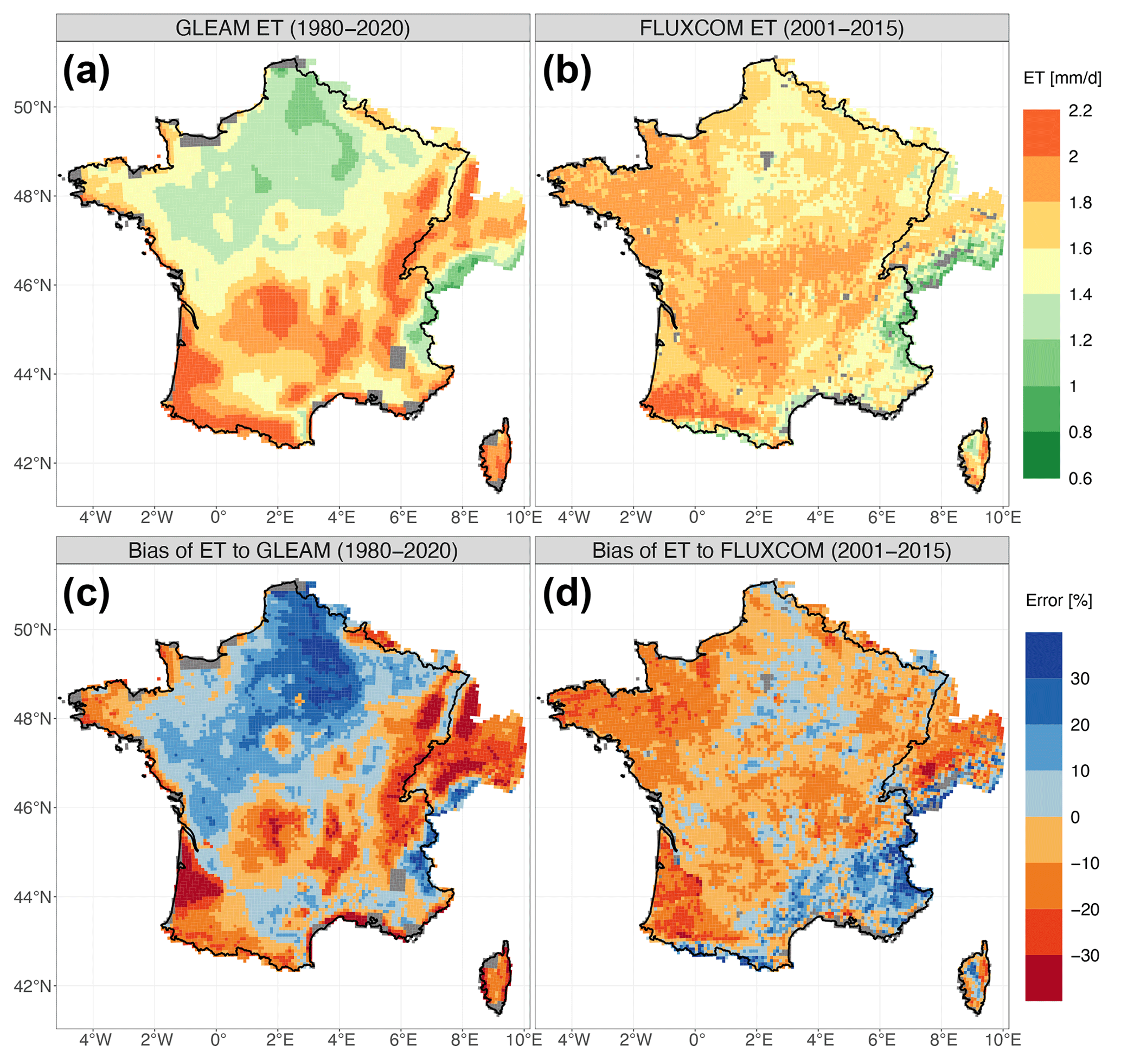
Figure 4 The spatial distributions of the ET datasets and the simulated ET biases against them for all the SAFRAN grid cells over the entire simulation domain: (a) the mean ET of the GLEAM dataset and (c) the bias of the simulated ET against it from 1980 to 2020 and (b) the mean ET of the FLUXCOM dataset and (d) the bias of the simulated ET against it from 2001 to 2015. The mean ET of the GLEAM dataset from 2001 to 2015 is not shown here but is very similar to that of the 1980–2020 period.

Figure 4c shows that the spatial distributions of the simulated ET biases are distinctly contrasted from those of the GLEAM dataset over the entire simulated domain: the simulated ET is generally underestimated in the mountainous regions (except for the high Alps, where a considerable overestimation occurs) and the Gascony region (alluvial plain of the Pyrenees) but is significantly overestimated in the northwestern part (notably the Seine River basin). On the other hand, compared to the FLUXCOM dataset, Fig. 4d shows that the simulated ET bias is generally underestimated but overestimated in the southeastern part of the entire simulation domain (notably the Mediterranean mountainous regions). Although the median bias of the simulated ET against GLEAM (−0.5 %) is better than that against FLUXCOM (−4.3 %), as illustrated in Fig. 3, the simulated ET is more spatially consistent with FLUXCOM.

3.3.2 Q simulation performance

Figure 5 shows the spatial distribution of the simulated Q criteria evaluated by the 1785 selected hydrometric stations in the HydroPortail dataset. The Q simulated by ORCHIDEE is mainly underestimated in Mediterranean river basins and overestimated elsewhere, which is consistent with the overestimation of the simulated ET in the Mediterranean region and the underestimation elsewhere against the FLUXCOM dataset. The biases of the simulated Q for most basins larger than 10³ km² are less than 10 %. In general, the river discharge levels in the Saône (a major tributary contributing to the Rhône River basin), Garonne and Loire River basins along the main river networks are satisfactorily represented by ORCHIDEE, with the Pearson correlation and KGE criteria mostly larger than 0.8 and 0.75, respectively. Subbasins with areas less than 10³ km² in these river basins are also fairly well simulated, with Pearson correlation and KGE criteria broadly larger than 0.6 and 0.5, respectively. In terms of the time lag criterion, most simulated Q values with large time lag errors correspond to catchments smaller than 10⁴ km², with simulated Q leading the observations by 2 to 6 d in the Seine River basin but lagging the observations by 2 to 4 d in the Loire River basin. The simulated Q values in the Garonne and Rhône River basins generally reveal no obvious leading or lagging results.

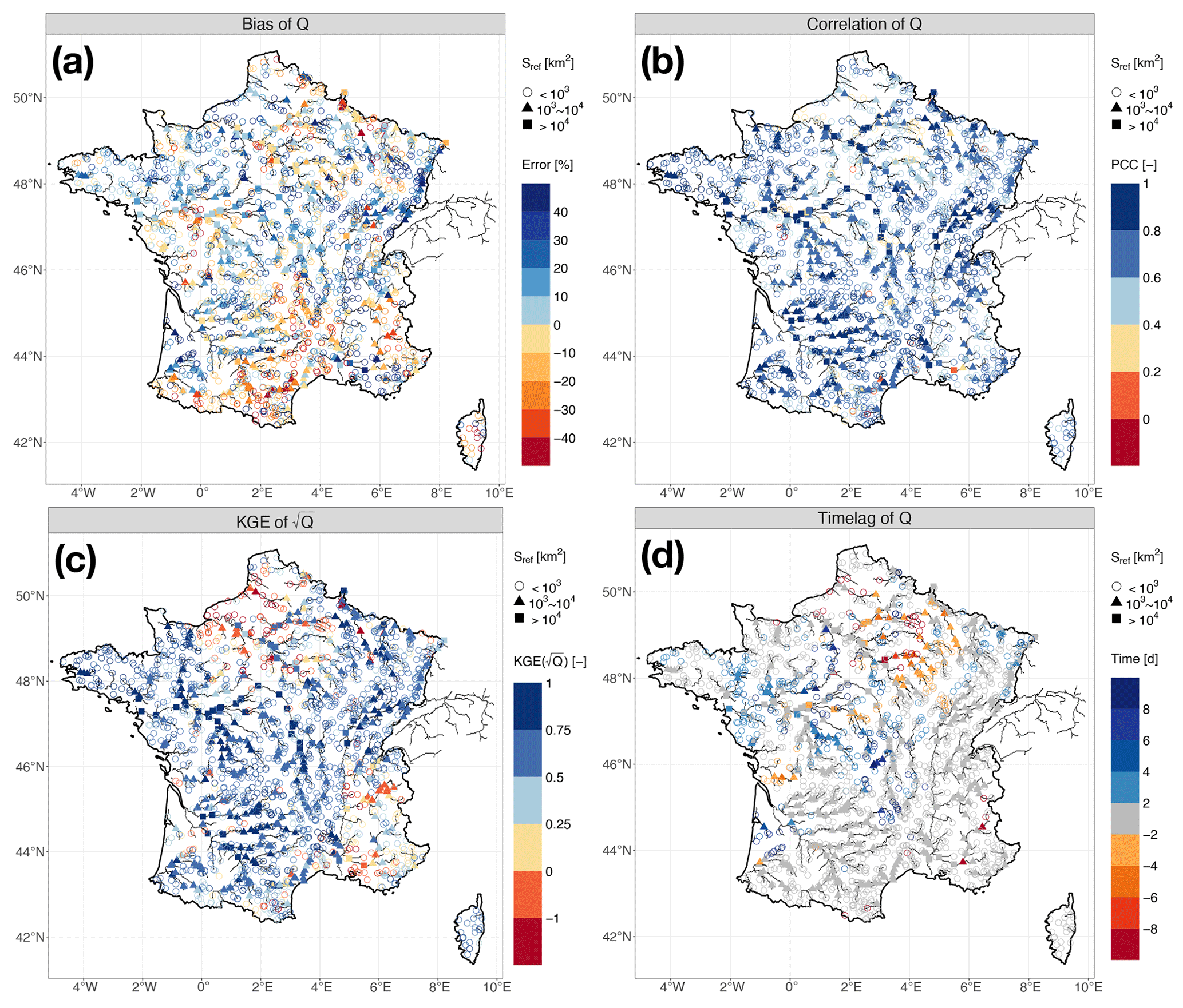
Figure 5 The spatial distribution of the Q simulation performance evaluated by the (a) bias, (b) Pearson correlation coefficient, (c) KGE of the square-rooted Q, and (d) time lag for the 1785 selected French hydrometric stations in the HydroPortail dataset over the entire simulation domain.

Human impacts on water that are not explicitly taken into account in this study lead to the degradation of goodness-of-fit indicators. An example of the simulation results for the Loire River basin is illustrated in Fig. 6. The variability and seasonality of the Q and ET fluxes are well represented by ORCHIDEE, while the simulated Q of the Loire River during the summer period is overestimated. This difference may be attributed to the irrigation extraction of maize crops by upstream reservoirs (Janin, 1996). The Seine River basin is influenced by upstream reservoirs that store high winter flows and release them during summer to meet environmental and navigational needs and by groundwater pumping mostly for drinking water in Paris (Flipo et al., 2020). These human interventions are not described in the ORCHIDEE LSM, which probably explains to a large extent why river discharge downstream of Paris is strongly underestimated, especially in summer (Fig. 7). In addition, the mountainous basins in the Alps (e.g. the Isère and Durance River basins, contributing to the Rhône River) and the Pyrenees (e.g. the Neste River basin, contributing to the Garonne River) show unsatisfactory simulation performance (Fig. S10 and S11) because these river basins are significantly perturbed by dams and reservoirs for winter hydropower production, spring refill and summer irrigation (e.g. the Serre-Ponçon reservoir in the Durance River basin, one of the largest dams in Europe) (François et al., 2014; Andrew and Sauquet, 2017; Huang et al., 2022; Baratgin et al., 2024). Figure S14 shows that ORCHIDEE performs better in natural or weakly influenced river basins than in human-influenced river basins, especially for correlation and KGE criteria.

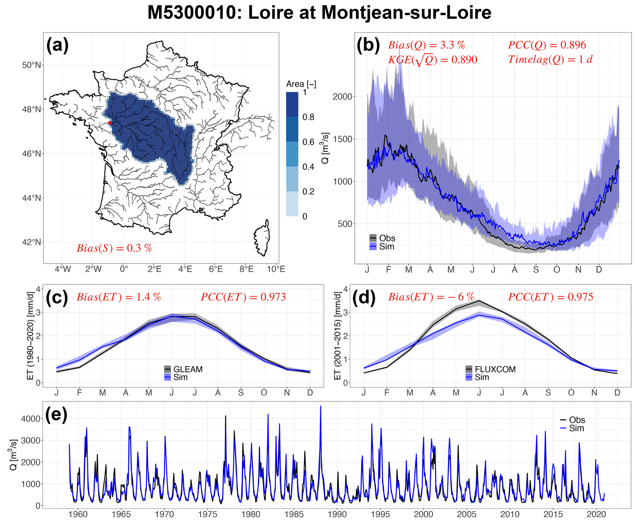
Figure 6 The simulation performance of the Loire River at the hydrometric station Montjean-sur-Loire (M5300010): (a) the simulated river basin area with the legend of the proportion of SAFRAN grids contributing to the basin area, (b) the annual regime of simulated Q compared to the observation in the HydroPortail dataset at a daily time step from 1959 to 2020, (c) the annual regime of simulated ET compared to the GLEAM dataset at a monthly time step from 1980 to 2020, (d) the annual regime of simulated ET compared to the FLUXCOM dataset at a monthly time step from 2001 to 2015 and (e) the simulated Q compared to the observation at a monthly time step from 1959 to 2020. The regime plots of ET and Q are presented with the color bands as the range between the 25 % and 75 % quantiles and the solid lines as the medians.

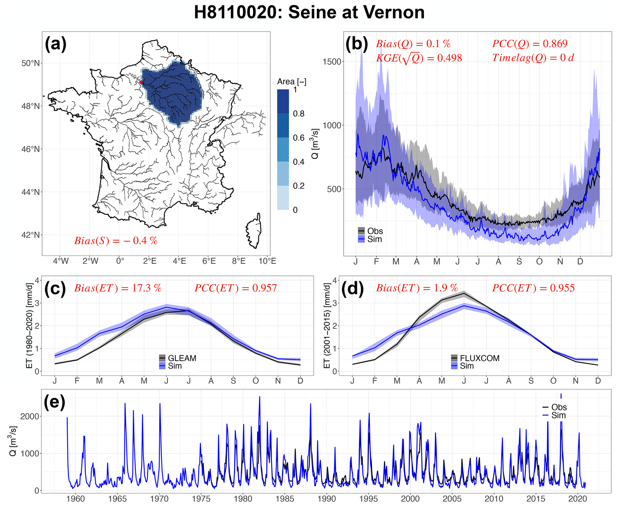
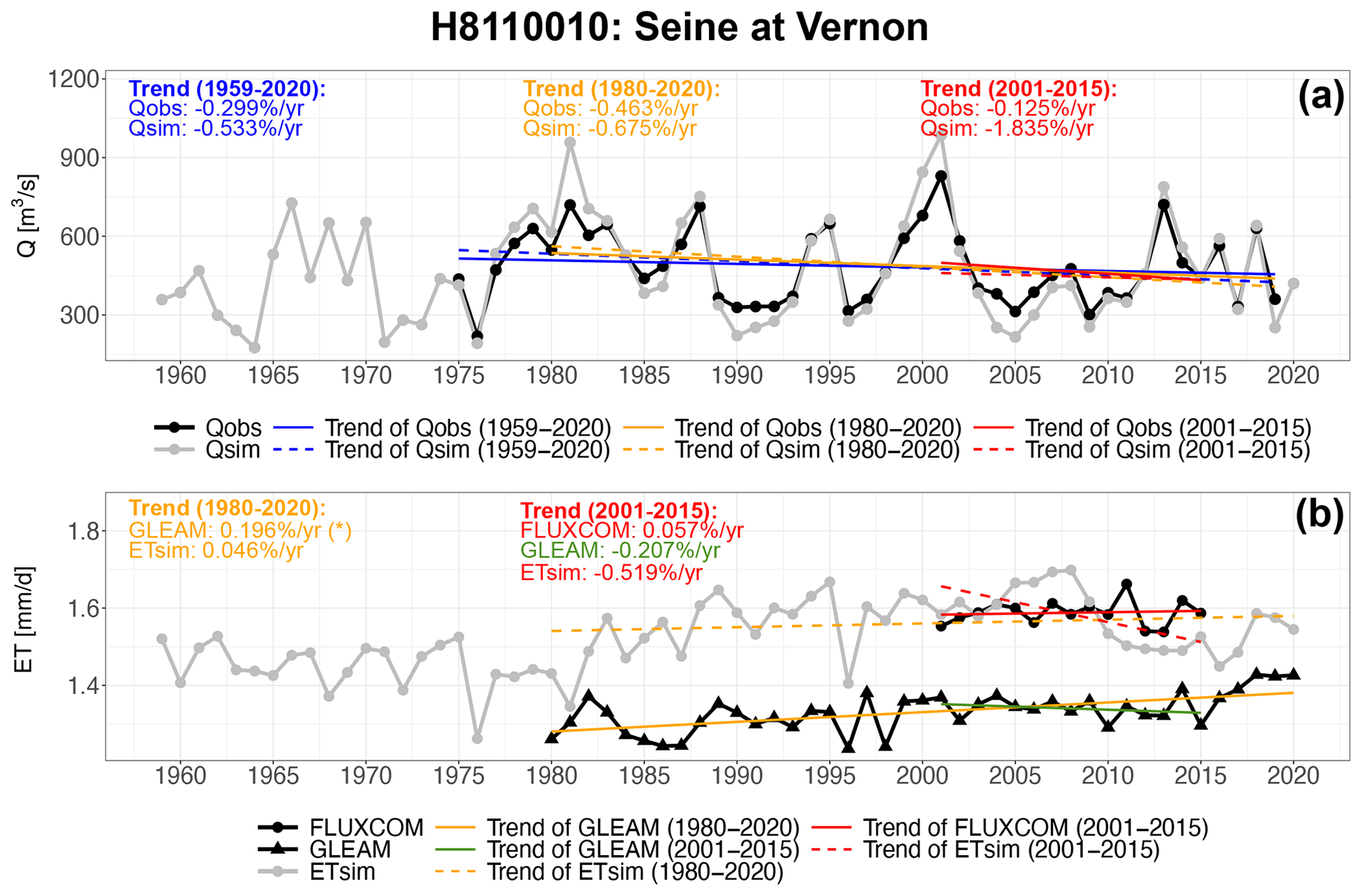
Figure 7 The same as in Fig. 6 but for the Seine River at the hydrometric station Vernon (H8110020).

Other model imperfections degrade the quality of simulated river discharge. In the mountains, these poor results could also be related to poor snow simulation. Groundwater is also known to strongly influence streamflow, especially in river basins embedded in sedimentary basins (e.g., the Seine River basin). Groundwater is simply represented in ORCHIDEE by the slow reservoir of the routing scheme as a free aquifer. However, ORCHIDEE does not account for the difference between large aquifers, which significantly buffer river discharge variability (Gascoin et al., 2009), and smaller aquifers, with shallow and very reactive water tables. This degrades ORCHIDEE's performance (e.g., bias and time lag) in the sedimentary basins. This problem could be approached by assigning larger residence times to the slow reservoirs of grid cells in sedimentary basins. However, it is difficult in practice because parameters are applied uniformly over France in ORCHIDEE.

3.4 Preferred experiment: evaluation of river discharge trends

Figure 8 shows that the calibrated ORCHIDEE LSM satisfactorily represents the observed Q trend of the 1785 selected French hydrometric stations. In general, both the observed and simulated Q trends exhibit similar spatial patterns, with a decreasing trend (significant) in the southeastern part of France and an increasing trend (not significant) in the northwestern part of France, which is consistent with the findings of previous studies (e.g., Gudmundsson et al., 2017; Vicente-Serrano et al., 2019). Most basins with significant observed and simulated decreasing trends are located in the Garonne River, upstream of the Loire River and upstream of the Rhône River. However, compared with the observed Q trends over France, the simulated Q trends tend to alleviate the decreasing trend and to enhance the increasing trend. For example, there is a general decreasing trend, usually not significant, for the basins located on the Mediterranean coast (including Corsica) from the observed Q, while the simulated trends are more variant. In the northwestern part of France (such as in the middle part of the Seine River and the Brittany Peninsula), the increasing trends of the simulated Q are more pronounced than in the observations. To summarize, the simulated trends tend to be more positive than the observed trends over France, which might be attributed to the fact that intensified water withdrawals (for irrigation, industry, and drinking water) are not considered in the simulation from 1959 to 2020. This period corresponds to the expansion of agricultural and water infrastructure projects across France (Janin, 1996), and human activities are inferred to be the dominant drivers of river flow decreases and drought aggravation (e.g., García-Ruiz et al., 2011; Loon et al., 2022; Greve et al., 2023). Nonetheless, climate variability and land use and land cover changes are taken into account in the simulations of this study, which partially explain the southeast–northwest (dry–wet) contrast across France.

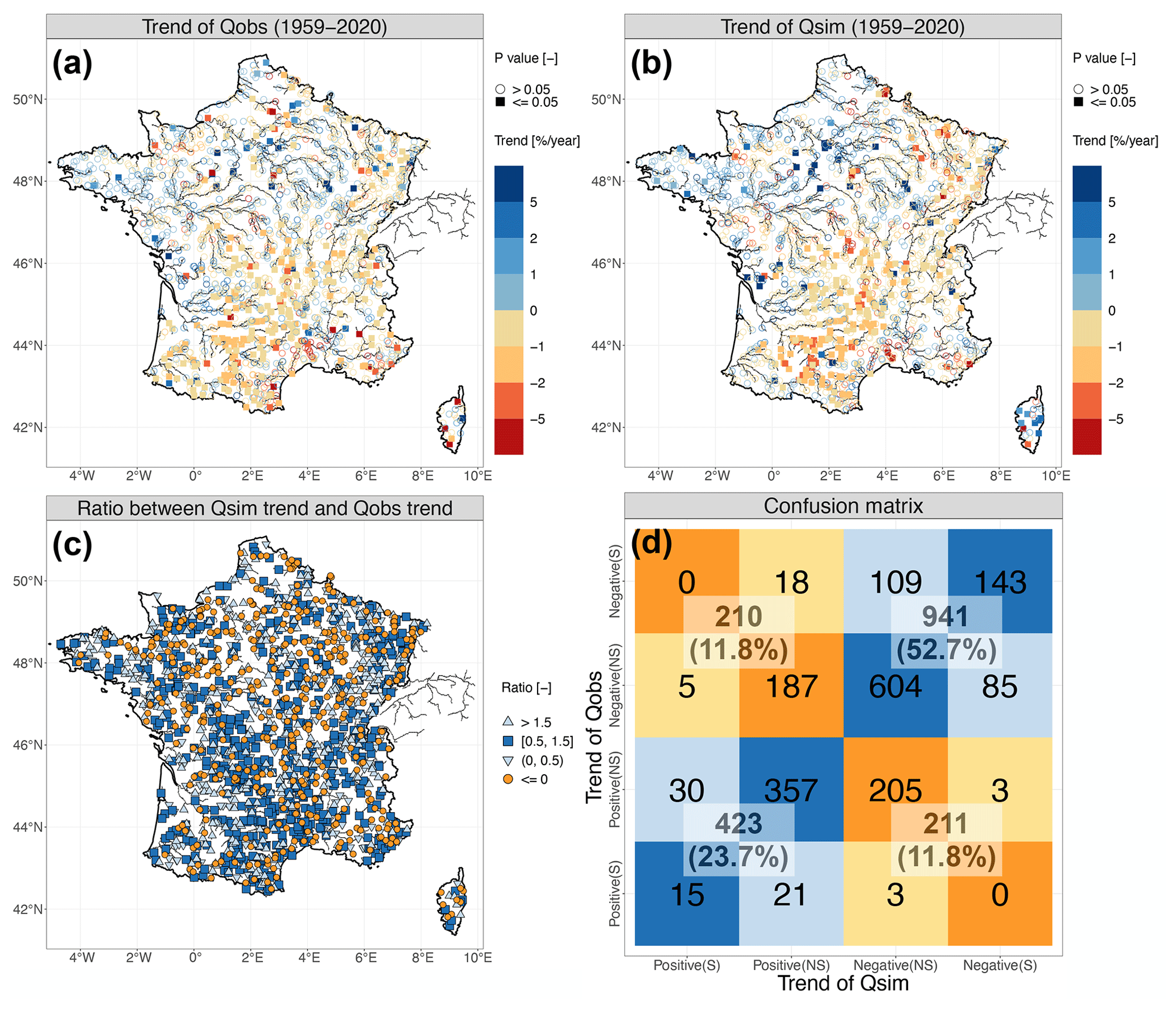
Figure 8 The spatial distribution of the observed Q trend (a), the simulated Q trend (b), and the ratio between the simulated Q trend and observed Q trend (c) for the 1785 selected French hydrometric stations in the HydroPortail dataset from 1959 to 2020. The trends of the simulated and observed Q are calculated with the yearly mean Q time series for the common period of the two time series. The confusion matrix (d) between the observed Q trend and the simulated Q trend is presented at four dimensions as colorful boxes (significant positive, not significant positive, not significant negative and significant negative) and at two dimensions as white boxes (positive and negative).

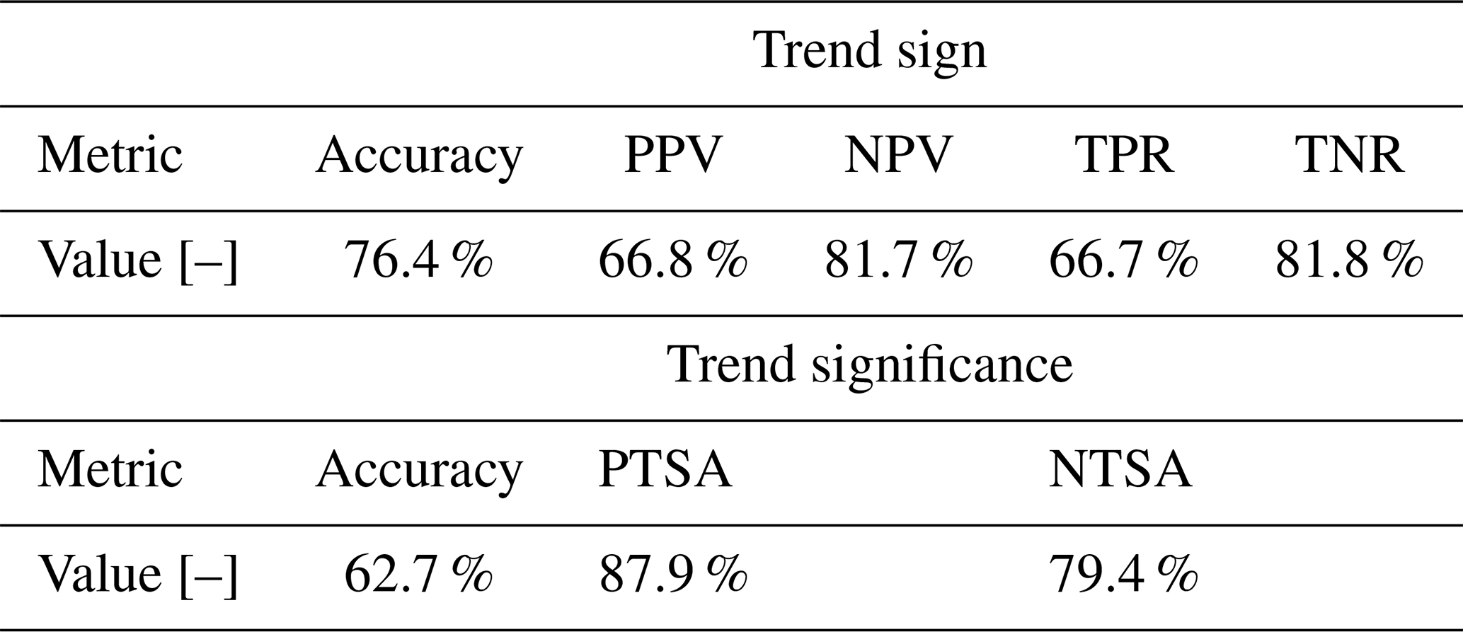
To further advance the information obtained from the confusion matrix of Fig. 8d, Table 2 summarizes the performance of the simulated Q trend sign and its significance with accuracy of the trend sign = $(\mathrm{941}+\mathrm{423})/\mathrm{1785}$, PPV = $\mathrm{423}/(\mathrm{423}+\mathrm{210})$, NPV = $\mathrm{941}/(\mathrm{941}+\mathrm{211})$, TPR = $\mathrm{423}/(\mathrm{423}+\mathrm{211})$, TNR = $\mathrm{941}/(\mathrm{941}+\mathrm{210})$, accuracy of trend significance = $(\mathrm{143}+\mathrm{604}+\mathrm{357}+\mathrm{15})/\mathrm{1785}$, PTSA = $(\mathrm{357}+\mathrm{15})/\mathrm{423}$ and NTSA = $(\mathrm{143}+\mathrm{604})/\mathrm{941}$. Generally, the ORCHIDEE LSM satisfactorily reproduces the past trends of French river discharge from 1959 to 2020, with an accuracy of 76.4 % for the trend sign and an accuracy of 62.7 % for the trend significance. Compared to the observed Q trend sign over France, the negative Q trend is relatively better simulated than the positive Q trend despite the inadequate consideration of human perturbations. However, in terms of the simulation performance of trend significance, the positive Q trend significance is slightly better than the negative Q trend significance.

Table 2 The confusion matrix metrics (detailed in Sect. 2.3) that evaluate the performance of the ORCHIDEE LSM in representing the Q trend sign and significance over France from 1959 to 2020 calculated from Fig. 8d.

Figures 9 and 10 show the water flux trends in the Loire and Seine River basins, respectively, as two examples. The decreasing trends of the annual streamflow for both river basins are well simulated by the ORCHIDEE LSM. Nevertheless, the simulated decreasing trend of the Loire River is weakened with the underestimation of wet years, while that of the Seine River is aggravated with the overestimation of wet years and the underestimation of dry years. The simulated increasing trends of ET for both river basins are more consistent with those of the GLEAM dataset than those of the FLUXCOM dataset given its longer records. More examples of the water flux trends are provided in the Supplement (Figs. S12 and S13).

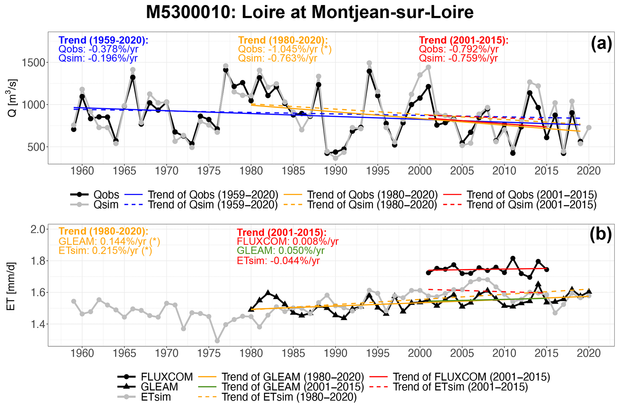
Figure 9 The temporal trends of the observed and simulated annual Q (a) and ET (b) of the Loire River at the hydrometric station Montjean-sur-Loire (M5300010) for the 1959–2020, 1980–2020 and 2001–2015 periods. The trend magnitudes are marked in the plots in units of percent per year, and the symbol (^*) indicates the significance of the trend (p value < 0.05).

Figure 10 The same as in Fig. 9 but for the Seine River at the hydrometric station Vernon (H8110010).

4 Discussion and conclusions

This study presents the development of a hydrological simulation with a high resolution of approximately 1.3 km over France with the ORCHIDEE LSM to quantify water resources at the nationwide scale, either retrospectively, as shown here to evaluate the setup, or prospectively, as planned for the Explore2 project to deliver climate change projections. After several calibration steps to improve the simulated water budget and hydrological performance, the simulation results over the 1959–2020 period are evaluated via comparison with the ET products (the GLEAM and FLUXCOM datasets) at monthly steps and with the French national hydrometric networks (the HydroPortail dataset) at daily time steps. Generally, the selected parameterization of the ORCHIDEE LSM provided satisfactory results in terms of the simulated basin areas and water fluxes.

This study emphasizes the ability of this version of ORCHIDEE to reproduce the temporal and spatial patterns of Q trends, with an accuracy of the trend sign of 76.4 % and that of the trend significance of 62.7 % over France. The decreasing trend in southeastern France with marked significance and the increasing trend in northwestern France with minor significance are adequately represented by the ORCHIDEE LSM. To a greater extent, this diagnosis is necessary for climate change impact studies because adaptation strategies are grounded in the statistical analysis of the projections, the potential trends of future river discharge in particular. Therefore, hydrological models must be able to accurately reproduce trends under current climate conditions. However, in most climate change impact studies, this investigation of hydrological model performance has been rarely analyzed but has been found to depend primarily on traditional goodness-of-fit indicators (e.g., KGE). A recent study revealed that these traditional indicators do not ensure the reproduction of trends (Todorović et al., 2022). An inadequate representation of vegetation dynamics can explain why some hydrological models fail to accurately reproduce river discharge trends (e.g., the HBV conceptual hydrological model; Duethmann et al., 2020). On the other hand, the incorporation of vegetation dynamics into hydrological models often improves their hydrological simulation performance (e.g., Jiao et al., 2017; Bai et al., 2018). The ORCHIDEE LSM accounts for the interactions between the biosphere (15 PFTs in this study) and hydrosphere (e.g., transpiration, precipitation interception, and photosynthesis) by coupling the SECHIBA and STOMATE modules to explicitly simulate the phenomena of the terrestrial carbon and water cycles (Ducoudré et al., 1993; Krinner et al., 2005).

The limitations of the modeling framework proposed in this study and the prospects to improve ORCHIDEE simulations are analyzed from these three major aspects: parameter calibration, input and evaluation datasets, and ORCHIDEE model structure.

First, uncertainties remain in the selected parameter set. In this study, we applied the trial-and-error calibration method (no parameter optimization procedure) to reduce the computational burden. The general principle of calibration is to decrease the biases of water fluxes across France by increasing ET and decreasing Q simulations starting from the CMIP6 configuration; the calibration experiments follow this principle by changing the parameters employed for all the grid cells across France. This procedure indeed simplifies the calibration of such sophisticated physically based LSMs to obtain generally accepted performance criteria over the entire simulation domain. However, improvements in simulation performance in some areas remain limited. For example, calibrating the hydraulic conductivity influenced by both soil and vegetation (EXP2 and EXP4) to adjust infiltration and surface runoff has improved the overall performance criteria, except for those of the Seine River basin. In reality, the characteristics of the Seine River basin, such as its relief and lithology, allow more predominant infiltration than surface runoff, especially in the upstream region of the Seine basin (e.g., Schneider et al., 2017; Mardhel et al., 2021). The calibration of soil hydraulic conductivity at the basin scale (i.e., different parameter values for the grid cells over the simulation domain) could improve the simulation results (e.g., Quintana Seguí et al., 2009). Another challenge is the parameterization of the 15 PFTs in terms of their transpiration capacity when facing water stress and root profiles (EXP3 and EXP4) due to the lack of observations, notwithstanding their importance to terrestrial carbon and water cycles.

Second, uncertainties concerning the input and evaluation datasets should also be considered. For instance, heterogeneity regarding the radiation data of the SAFRAN reanalysis (i.e., the break of homogeneity in time series with an abrupt increase in the profile of incident solar radiation after the late 1980s) has been reported, which could be attributed to the improvement of the assimilation system over time, the variation of the in situ observations and the darkening–lightening effect (e.g., Le Moigne et al., 2020). This directly impacts the ET simulation results. There are also large uncertainties in the SAFRAN reanalysis on precipitation in high-elevation areas in France (e.g., Birman et al., 2017; Baratgin et al., 2024). The uncertainties of other input datasets, such as the Reynolds soil texture map and the LUH2 land use and land cover maps applied to the ORCHIDEE LSM, have been discussed in other studies (e.g., Kilic et al., 2023; Lurton et al., 2020; Tafasca et al., 2020). In addition, Q records of the selected 1785 stations are not fully checked because identifying Q anomalies is extremely time-consuming and subjective. The remaining observational Q errors might influence model evaluation.

Third, some perspectives concerning better representations of land surface processes can be proposed to improve the simulation performance of the ORCHIDEE LSM. Given the inadequate performance of basins where drainage plays an important role in river discharge (e.g., the Seine River basins), the introduction of a groundwater module in the ORCHIDEE LSM is necessary to describe the interactions between aquifers and rivers in these basins. Moreover, mountainous basins are not adequately simulated; indeed, the SAFRAN reanalysis is deficient in these regions, and there is still room for improvement in the three-layer snow model, especially for the snow thermal conductivity, which is crucial for snow dynamics (Wang et al., 2013). Human impacts on terrestrial water cycles could also be included to obtain more reliable simulations by comparison to the observations in highly anthropized basins. In particular, a new irrigation module based on the flooding irrigation method (Arboleda-Obando et al., 2024) and a new demand-based hydropower module (Baratgin et al., 2024) have recently been developed and validated by the ORCHIDEE project team at IPSL and should now be mobilized to achieve more realistic simulations.