Exploring the provenance of information across Canadian hydrometric stations: implications for discharge estimation and uncertainty quantification

Accurate discharge values form the foundation of effective water resource planning and management. Unfortunately, these data are often perceived as absolute and deterministic by users, modelers, and decision-makers, despite the inherent subjectivity and uncertainty in the data preparation processes. This study is undertaken to examine the discharge estimation methods used by the Water Survey of Canada (WSC) and their impacts on reported discharge values. First, we explain the hydrometric station network, essential terminologies, and fundamental concepts of rating curves. Subsequently, we examine WSC's standard operating procedures (SOPs), including shift, temporary shift, and override, in discharge estimation. Based on WSC's records of ∼ 1800 active hydrometric stations for discharge monitoring, we evaluated sample rating curves and their correlation with stage and discharge measurement. We investigate under-ice measurements, ice condition periods and frequency, and extreme values in contrast to rating curves. Employing an independent workflow, we demonstrate that 69 % of existing records align with the rating curve and temporary shift concept, while the remaining 31 % follow alternative discharge estimation methods (override). Selected example stations illustrate discharge estimation methods over time. We also demonstrate the impact of override and temporary shifts on commonly assumed uncertainty models. Given the practices of override and temporary shifts within WSC, there is a need to explore innovative methods for discharge uncertainty estimation. We hope our research helps in the critical challenge of estimating and communicating uncertainty in published discharge values.

1 Introduction

River discharge or streamflow is the fundamental data upon which hydrology and water management depend (McMillan et al., 2017; Shafiei et al., 2022). River discharge is the integration of other states and fluxes such as precipitation, evaporation, and soil moisture level at the catchment and basin scales and hence carries important information about natural and anthropogenic processes. Given this importance, national gathering of river discharge data is typically a data product that governments provide as basic national infrastructure to support decision-making, planning, and water management objectives of governments, industry, and private sectors.

River discharge values are typically obtained by using a relationship called a rating curve (Rantz, 1982) to convert measurements of stage (water level) into estimates of discharge (water volume over time). Direct discharge measurements are made using techniques such as velocity and flow meters or acoustic Doppler systems. Each measurement technique, device, frequency, and protocol results in various error magnitudes (Pelletier, 1989), contributing to discharge measurement uncertainties (Whalley et al., 2001; Cohn et al., 2013). Rating curves are developed through occasional field discharge measurements, where hydrographers relate these direct measurements to river stages. The structure of the residual model for rating curves can then be characterized by comparing these measurements to the rating curves. This residual model can subsequently be used, often following established methods, to estimate discharge uncertainty (Coxon et al., 2015; Kiang et al., 2018).

In addition, errors in discharge values also stem from the (limited) capability of rating curves to represent time-dependent changes in stage–discharge relationships. Such time-dependent changes in river conditions come from local hydrodynamic and environmental conditions. This includes time-dependent changes in river conditions that introduce backwater effects due to sedimentation, vegetation growth, or ice formation. The stage–discharge relationships defined by rating curves are generally functional forms, while in reality they may be hysteretic due to the dynamic nature of water movement in the channel (Tawfik et al., 1997; Wolfs and Willems, 2014; Lloyd et al., 2016; Gharari and Razavi, 2018). For example, the rising limb and falling limb of a flood hydrograph may exhibit different discharge values for the same stage. This difference between the assumed stage–discharge relationship and the dynamic nature of the stage–discharge relationship is a source of uncertainty (among many other sources of discharge uncertainty).

Lastly, standard operating procedures or SOPs that are developed and used by hydrometric agencies for translating water level to discharge are often established for constant reassessment. In many instances, the stage–discharge relationship can be subject to the hydrographers' intervention. As an example, the process of creating a rating curve from observational discharge measurement may need to follow agreed-upon institutional or organizational procedures. In addition, updating rating curves over time to try to maintain the accuracy of relationships may result in more challenges in uncertainty quantification associated with the rating curve.

Given the differences in operating procedures, separating the above sources of uncertainty quantitatively is challenging and needs an extensive understanding of the operating procedures to determine the magnitude of each of the sources of uncertainty. Despite this difficulty, the communication of the discharge uncertainty is becoming increasingly important as hydrological, water quality, and water management models, which are often used for decision-making, are based on these published and approved estimates of river discharge.

This study seeks to identify critical decisions on discharge estimation processes at the Water Survey of Canada (WSC). The study tries to address the following questions:

• What are the standard operating procedures followed by hydrographers for discharge estimation?

• What are the critical decisions that affect discharge estimation and the associated uncertainties, and how can they be categorized?

• How can access to metadata and measurements be improved to aid in the estimation of discharge uncertainty for Canadian hydrometric stations?

The response and investigation of the aforementioned questions serve as the foundation for the overarching objectives of standardizing uncertainty quantification and communication within the quality assurance and management system, QMS, of WSC.

This paper is organized as follows. First, the terminologies are introduced to familiarize readers with the institutions, SOPs, and concepts used in this study as well as the workflow from data acquisition to river discharge estimation. This is followed by the “Results” section, where examples of rating curves and their relationship with observations of stage–discharge values are discussed. The discharge values estimated by WSC are reproduced using the available stage values and information in the production system. The paper concludes by discussing the findings and suggestions for essential data acquisition and archiving that will allow for better uncertainty estimation for Canadian hydrometric stations.

2 Data, terminologies, and methodologies

2.1 Canada's hydrometric monitoring program

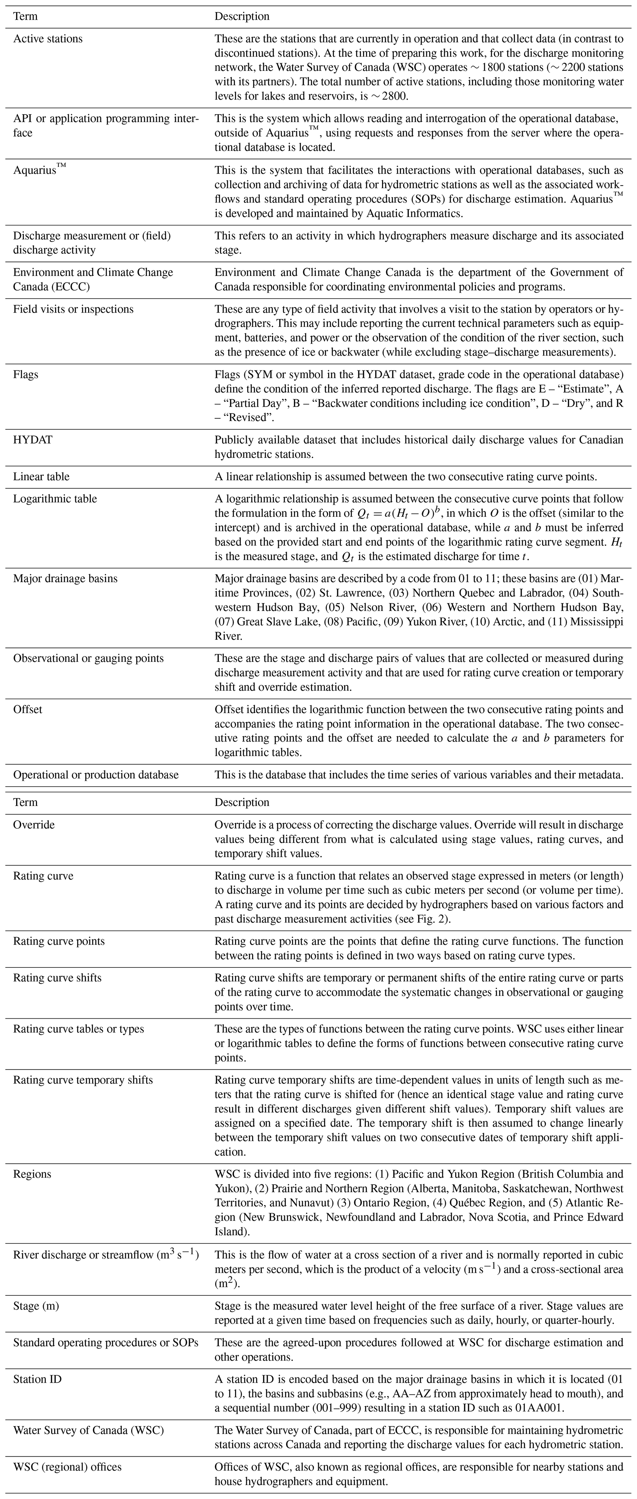
Canada, like many other nations, has invested heavily in its national hydrometric monitoring program through WSC and in publicly available national service and historic discharge records (refer to Table A1 for the terminologies that are used in this work). WSC is a unit of the National Hydrological Service for Canada, which is housed within the Canadian Government and is part of the Federal Department of Environment, known as Environment and Climate Change Canada (ECCC). WSC, an ISO-9001-certified organization, oversees the collection, harmonization, and standardization of discharge information in a cost-shared partnership with provincial and territorial governments across Canada. WSC divides its data into five regional entities: the (1) Pacific and Yukon Region (British Columbia and Yukon), (2) Prairie and Northern Region (Alberta, Manitoba, Saskatchewan, Northwest Territories, and Nunavut), (3) Ontario Region, (4) Québec Region, and (5) Atlantic Region (New Brunswick, Newfoundland and Labrador, Nova Scotia, and Prince Edward Island). The Ministère de l'Environnement, de la Lutte contre les changements climatiques, de la Faune et des Parcs operates the majority of Quebec's hydrometric stations and contributes these data to the national database under cost-share agreements and partnerships. Other provinces also operate their stations and contribute to the network. WSC monitoring stations include measurements in real time of water levels in lakes and rivers and real-time river discharge estimation for the majority of its active stations. WSC, currently, operates approximately 1800 active stations across Canada for discharge monitoring (refer to the active stations in Table A1). The number of active stations has changed over time, while some historical stations are discontinued (not active currently). Detailed descriptions of the history of WSC, its partnership, and its technical evolution are documented (Halliday, 2008; Kimmett, 2021).

2.2 Overview of the current production system

WSC uses the Aquarius^™ operation system maintained and operated by Aquatic Informatics. Aquarius^™ is used for interaction with the operational database and manipulation of values for discharge estimation. This system was tailored to the WSC SOPs and QMS and has been in use since 2010. The Aquarius^™ system allows for real-time water level reporting and flow data estimations for most WSC stations equipped with telemetry systems. Aquarius^™, including its graphical user interface or GUI, provides many options to hydrographers to revise the discharge values, smoothen discontinuities, and fill gaps, among others.

The most important variable in hydrometry is the stage or water level. Accurate measurement of stage values is crucial as this is the main variable used in combination with the rating curve to estimate discharge. The recorded stage values are at temporal resolutions programmed into the field-based logger system and are typically on the order of minutes. It is worth mentioning that, although in the past the stage observation temporal resolution would vary between sites and span from daily, hourly, half-hourly, or quarter-hourly, the stage logger time steps are currently set at 5 min. The collected stage values go through automated checks to account for faulty readings and are used, with the help of rating curves, to estimate discharge values. These provisional discharge data are later quality-assured and approved using a rigorous approval process. The approval process, among others, includes the repeatability of estimated discharge values by other hydrographers. The reported discharge values are accompanied by quality assurance flags that identify the condition under which the river discharge is estimated (explained in Table A1). The aggregated discharge values at daily temporal resolution are disseminated publicly through the National Water Data Archive of Canada called HYDAT.

There is information in the production database regarding field visits and stage–discharge measurements. Field visits are activities that are designed to ensure the operational integrity of instruments at a station. Stage–discharge measurements encompass activities using techniques such as mid-section using standard flow meters or acoustic Doppler equipment for river discharge measurement. In practice, multiple discharge measurements are made to determine a consistent flow estimate, particularly when the measured discharge deviates substantially from the expected discharge estimate derived from the rating curve (stage–discharge relationship). The discharge measurement activities are essential for confirming or adjusting rating curves. Based on new discharge measurements or environmental factors such as the presence of ice, a hydrographer may decide to apply or change previously estimated discharge. Additionally, based on new stage–discharge measurements, hydrographers may decide to design and test new rating curves.

The earliest records of stage values in the current WSC operational database are from the mid-1990s. These data were transferred from the previous NewLeaf production system when Aquarius^™ was first introduced. The reader should note that what is contained in the operational database is only a fraction of the existing historical time series that exists in various forms at WSC regional offices or in earlier database systems. For example, for the Bow River at Banff station located in the province of Alberta, the stage and associated estimated discharge records start from 1995 in the operational database, while the reported discharge in the HYDAT dataset goes back to 1909. Similarly, the earliest records of observational field discharge measurements and the earliest rating curve recorded for each station in the operational database extend mostly to the 1970s and 1980s. For the same station, the existing rating curves in the operational database system began in 1990, despite over 100 years of records. Earlier rating curves cannot be accessed from the operational database as they have not been transferred to this system. However, all the records are available, many as hard copies in the WSC's regional offices. There is a similar story for historical field discharge measurements: not all the earlier historical observations have been carried over to the current operational database. For the Bow River at Banff station, the earliest observational discharge in the operational database is from 1986. The difference between the period of the digital operational database accessible by Aquarius^™ and records that exist at WSC regional offices needs to be emphasized since the present analysis is limited to data that are contained in the current operational database.

The focus of this study is only on active stations. Each station is defined by a station ID. The station ID is a unique identifier for each hydrometric station and its approximate location using a standard WSC naming convention. In this convention, the first two digits define the major drainage basin in which the station is located (01–11; see Fig. 1). The two digits are followed by two letters that define the locations of subbasins ordered from headwaters to the mouth of each major drainage basin (AA, BA, BB, BC, etc.). The ID ends with a three-digit sequential number of the stations in the subbasins. As an example, the station ID of the Bow River at Banff, 05BB001, indicates that it was the first station in subbasin BB that is located in the Saskatchewan or Nelson River basin and identified by the leading code of 05.

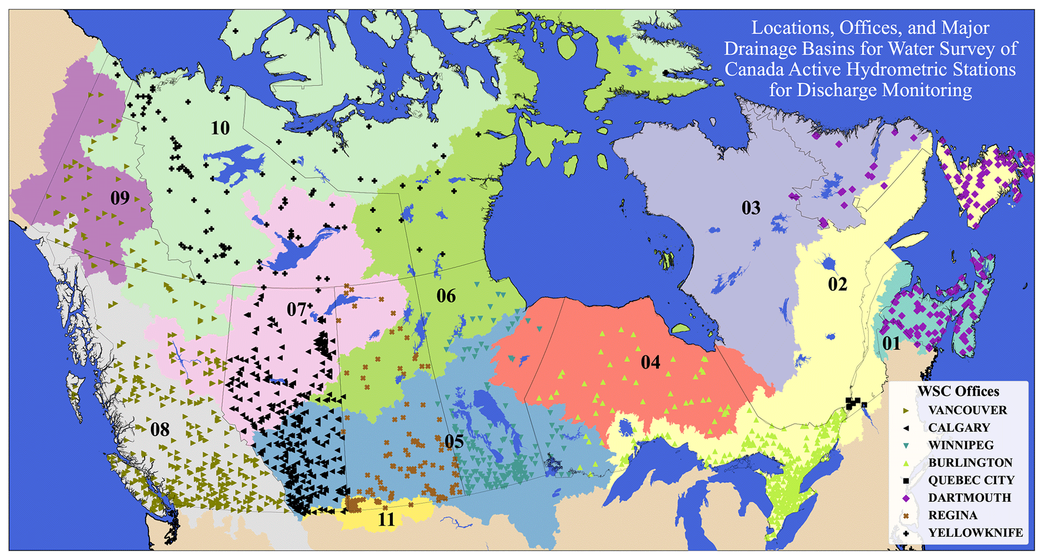
Figure 1 Locations of ∼ 1800 active stations for river discharge monitoring operated by WSC. The 11 major drainage basins are the (01) Maritime Provinces, (02) St. Lawrence, (03) Northern Quebec and Labrador, (04) Southwestern Hudson Bay, (05) Nelson River, (06) Western and Northern Hudson Bay, (07) Great Slave Lake, (08) Pacific, (09) Yukon River, (10) Arctic, and (11) Mississippi River. These digits are the first two characters in the station IDs. The Quebec stations that are operated by the Ministère de l'Environnement, de la Lutte contre les changements climatiques, de la Faune et des Parcs of the Province of Québec are not included in the WSC production database, nor are stations operated by other government agencies, whether they are crown or private corporations.

2.3 Rating curves

Rating curves are perhaps the most commonly used method for river discharge estimation derived from stage observations. Rating curves are functional hydraulic relationships that relate river stage values to discharge values. In the WSC operational database, each rating curve is tied to an effective period, from a start date to an end date, where the rating curve is considered the valid expression for estimating discharge values from stage records. Rating points are pairs of stage and discharge values that define the forms of rating curve functions (red points in Fig. 2a and b). For the interpolation between the two consecutive rating curve points, WSC uses two major approaches: (1) linear table and (2) logarithmic table. In a linear table, a linear relationship is assumed between the rating points (Fig. 2a), while in a logarithmic table a logarithmic relationship is used instead (Fig. 2b). The logarithmic relationship is defined by the form of $Q_t=a(H_t-O{)}^b$ with parameters a and b and an offset value of O. The offset values are archived alongside the rating points in the production system database, while a and b can be inferred using the position, read stage, and discharge of the consecutive rating curve points. H_t is the measured stage, and Q_t is the estimated discharge at time t. The logarithmic expression of the rating curve resembles the hydraulic equations relating water elevation to discharge. The offset, O, can also be referred to as the reference elevation or H₀ and alongside parameters a and b can reflect “hydraulic” characteristics (Reitan and Petersen-Øverleir, 2011).

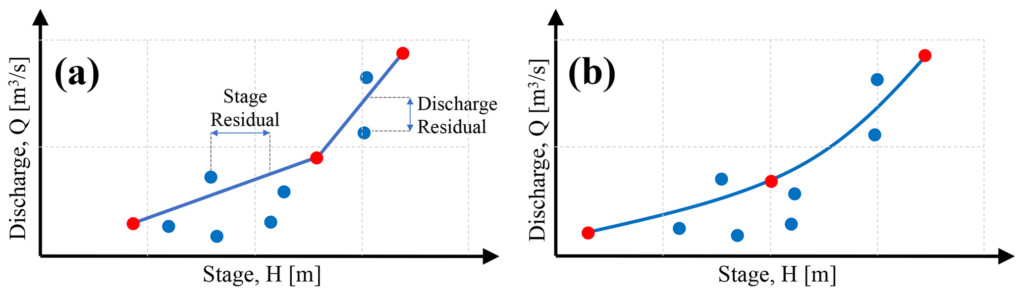
Figure 2 Examples of (a) linear table and (b) logarithmic table rating curves. The blue points are the observation points of the measured stage and discharge during discharge measurement; the rating points that define the rating curve are shown in red. In practice, these are not equations describing curves, but lookup tables that record stage and discharge values.

2.4 Managing rating curve changes

The process of managing changes that affect a rating curve can be broken down into three major practices, which are defined in the WSC standard operating procedures (SOPs). These changes can include nonfunctional relationships such as hysteresis or nonstationary relationships over time due to physical and environmental factors. The processes are itemized below.

• (Re)construction of rating curves. New observations that indicate a change in the local hydraulic realities may require the establishment of a new rating curve. A new rating curve is required when some or all of the historic stage–discharge observations do not fit new discharge measurements and cannot easily be accommodated by historical rating curve manipulations. Large changes to a water body or structural influences on local hydraulics may warrant this reconstruction. Another example would be the construction of a rating curve beyond the maximum observed stage–discharge observation using various types of modeling techniques or a change in the rating curve from a linear table to a logarithmic table.

• Shift. The shift of a rating curve happens when the entire rating curve or part of the rating curve needs to be adjusted based on new discharge measurements (but not entirely reconstructed). These shifts can have various forms; the simplest form is a constant or single point shift in which the new observational points show a single value shift in comparison to earlier observations and the rating curve (constant over the range of the rating curve). The other types of shift can be used to accommodate part of the rating curve shift, called the knee bend, or more local accommodation of changes in the rating curve by truss shift (Fig. 3). Readers are encouraged to refer to earlier works to read a more extensive elaboration of rating curve shift (Rainville et al., 2002; Mansanarez et al., 2019; Reitan and Petersen-Øverleir, 2011).

• Temporary shift. The concept of the temporary shift of rating curves is not widely known or explored in the literature. The temporary shift is the movement of a rating curve along its stage axis to adjust for the short-term presence of environmental disturbances such as backwater and ice conditions. Figure 4a–c show an example of how temporary shift is applied over time and how the application of temporary shift affects the inferred discharge compared to the case when temporary shift is not used for ice cover conditions. Figure 5 illustrates the effect of an applied temporary shift on the rating curve. Initially, the temporary shift is set to zero before time t₁, meaning that the stage–discharge relationship follows the original rating curve. There is a field measurement during this period. The newly obtained stage and discharge values during the field measurement do not conform to the rating curve (residuals are not zero). In the next discharge measurement during the freeze-up period, the hydrographer, based on environmental conditions and the discharge measurement at t₂, will apply a negative temporary shift. The negative temporary shift can be either summed with stage values or represented by a rating curve temporary shift to the positive stage direction (and the other way round for positive temporary shift values). In this example, the rating curve is shifted to the right along the stage axis, which implies that, during the freeze-up period, identical stage values will result in a smaller discharge estimation in comparison to the original rating curve (when the temporary shift of zero means open water). The magnitude of this negative temporary shift is applied so that the observed stage and discharge at time t₂ coincide with the temporarily shifted rating curve (observation is given more weight, which results in zero residuals). The temporary shift in magnitude is increased at time t₃ based on the development of ice cover over the river. At time t₄ another discharge measurement is performed. The hydrographer decides to adjust the temporary shift value at this time, t₄, to match the observational stage and discharge (again giving more weight to the observation and setting the residuals to the minimum). Finally, during a field visit after the ice breaks up, the hydrographer reduces the temporary shift magnitude to be set to zero at t₆, after which the original rating curve is used. The temporary shift changes linearly between the date and time of application of each temporary shift value. This linear change over time essentially means that between the times of t₁ and t₆ there is effectively a new rating curve for every logger reading of stage values. The temporary shift values and their time and date of application are recorded in the operational database.

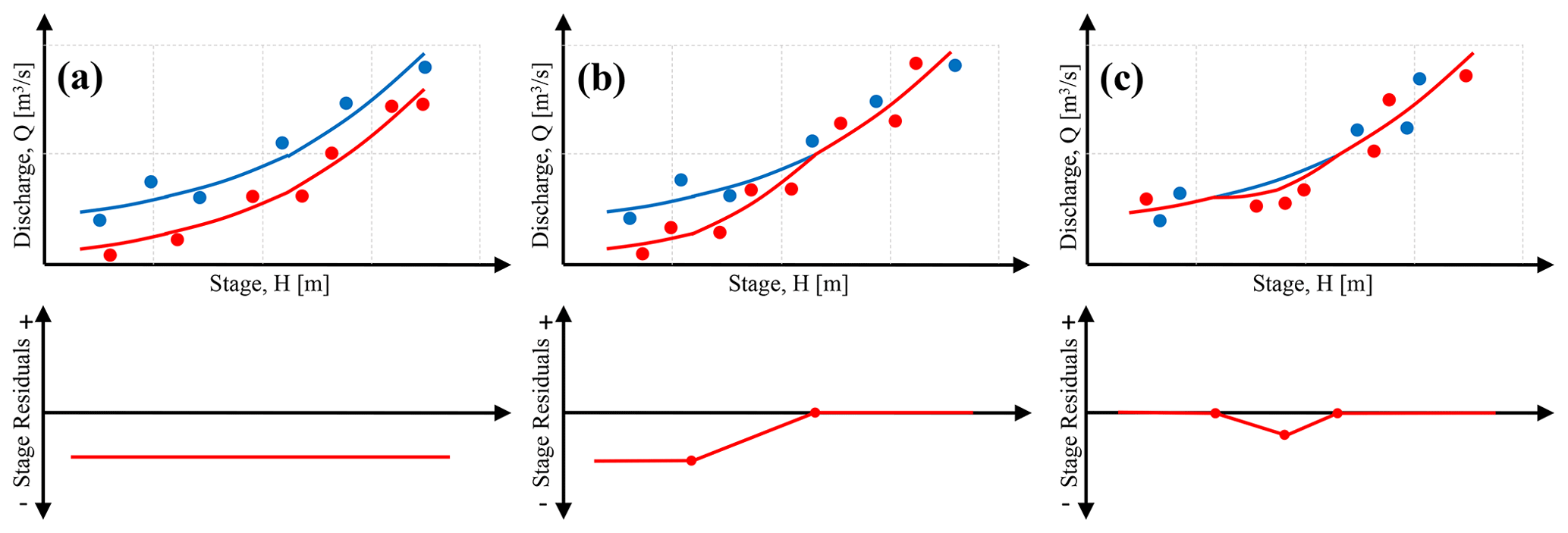
Figure 3 The shift in rating curve segments to accommodate new observation points based on stage residuals for various types from a base (original) rating curve: (a) constant or single point shift in which the rating curve is shifted with a constant value over its entire range, (b) knee bend in which part of the rating curve is shifted with a constant value, and (c) truss in which more local shift is applied on a rating curve.

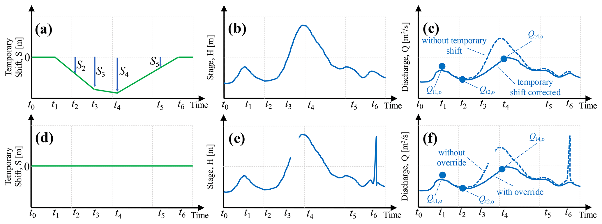
Figure 4 The top panels provide an example of discharge estimation using the concept of temporary shift. The bottom panels provide an example of discharge estimation using the concept of override (while the temporary shift is set to zero). (a) The evolution of temporary shifts over time, (b) stage time series, (c) estimated discharge time series with and without temporary shift, (d) temporary shift time series (set to zero), (e) the stage value record that has a gap and faulty reading, and (f) the estimated discharge values using override techniques that are corrected for the gap, discharge measurement, and faulty reading. The effect of temporary shift time series on the rating curve is illustrated in Fig. 5. The subscript “o” denotes “observational” discharge.

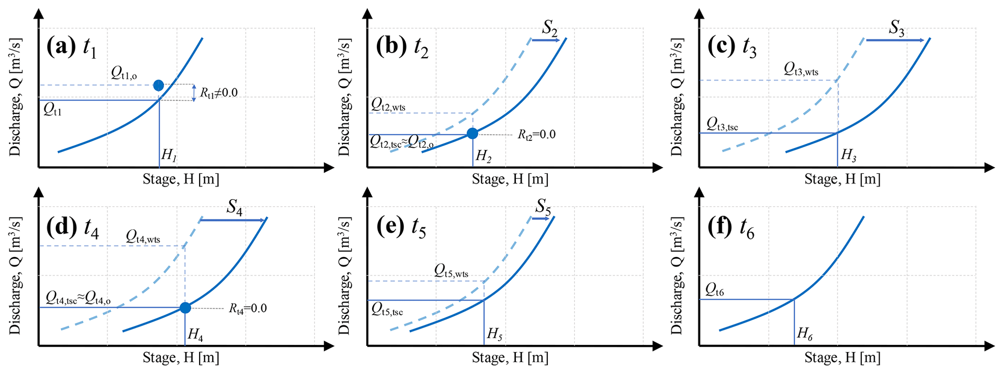
Figure 5 Temporary shifted rating curves at (a) t₁, (b) t₂, (c) t₃, (d) t₄, (e) t₅, and (f) t₆ from temporary shift time series illustrated in Fig. 4a applied based on the environmental condition during ice cover, hydrographer experience, and discharge measurements. The subscripts wst denote “without temporary shift” discharge, tsc “temporary shift corrected” discharge, and o “observational” discharge.

2.5 Overrides

In addition to the temporary shift of the rating curve, WSC uses other methods outside the manipulation of rating curves to report an updated discharge estimation. These updates follow WSC SOP rules and are based on a multitude of factors, e.g., discharge measurements and a hydrographer's judgment as to the state of changes in the river. The collective title of these efforts is override, in which WSC hydrographers use various techniques and sources of information to manually correct discharge values. Overrides may include adjustments based on upstream or downstream station readings, linear interpolation of missing values, reconstruction of peak discharge by (hydraulic) modeling, falling limp using decay functions, or under-ice discharge variations, among others. The override practices can sometimes vary between the WSC offices. Although the hydrographers at WSC follow SOP guidelines and their experience for this estimation, given that our efforts were limited to data available from the application programming interface (API), it is challenging to easily recreate estimated discharge values reported in the operational database. Figure 4d–f illustrate a very simplified example of an override in which the temporary shift is not used (and hence zero). The discharge values are manipulated to fill the gap between time t₃ and t₄ in the stage record for the rising limb of a flood event. The discharge values are also changed to reduce the estimated peak flow to better match the observational discharge at time t₄. Finally, the hydrographer decides that the stage reading values at t₆ are faulty and should not be used for discharge estimation. The discharge values for this faulty reading are then interpolated using the past and future readings of this station and possible existing upstream and/or downstream stations.

2.6 Developing an independent workflow

An independent Python workflow is designed to evaluate the reported discharge values in the operational WSC database. The designed workflow uses the API to extract data directly from the database. The main aim of the workflow is to replicate the reported discharge in the operational database, Discharge.Historical.Working, using the recorder stage values identified by Stage.Historical.Working together with other available information, such as rating curves and the temporary shift from the operational database. The workflow is designed in five steps: step 1 is the interrogation of the metadata from the production database. This includes downloading the metadata for available time series at logger resolution, such as stage, pressure, voltage, or any parameter that reflects the functionality of instruments or environmental factors. Information about the rating curves (their IDs) and the dates of their applications is also extracted. In the second step, step 2, rating curves and time series are downloaded from the production database. These data are the rating curve tables, including the offset for the logarithmic table and the effective temporary shift at a given date and time (specified in the temporary shift metadata from step 1). Step 3 is the adjustment of the variables to common scales. This includes refining the rating curves to increments of 1 mm for finer interpolation along the stage axis and also resampling and interpolating continuous or discrete information such as temporary shift values and rating curve IDs to temporal stage resolutions. This step provides the information needed to estimate the discharge from stage values. Step 4 mainly focuses on estimating discharge from the stage based on the files created from the adjustment step and the time series of stage values used to recreate discharge within the production system. Finally, step 5 of the workflow focuses on evaluating and interpreting the reproduced discharge and comparing it with the reported values from the production database. The difference between the reported discharge values in the production database, which contains override practices and values as well as reconstructed discharge based on the abovementioned workflow, can shed light on the level of possible intervention by override or other methods in reported discharge.

3 Results

3.1 Rating curve construction and characteristics

Rating curves are characterized by rating points, and in the case of a logarithmic table they are accompanied by offset values (O; refer to Table A1 and Fig. 2). Our findings, contrasting the rating curves and observational points, indicate that the creation of rating curves from observational points does not always follow a unified statistical approach. Rather, it is sometimes based on hydrographer judgment and field observations. Additionally, it is not apparent, when extracting data from the API system, which stage–discharge measurement points are used to update the current rating. A few of the limitations in reproducing rating curves are described below (Fig. 6).

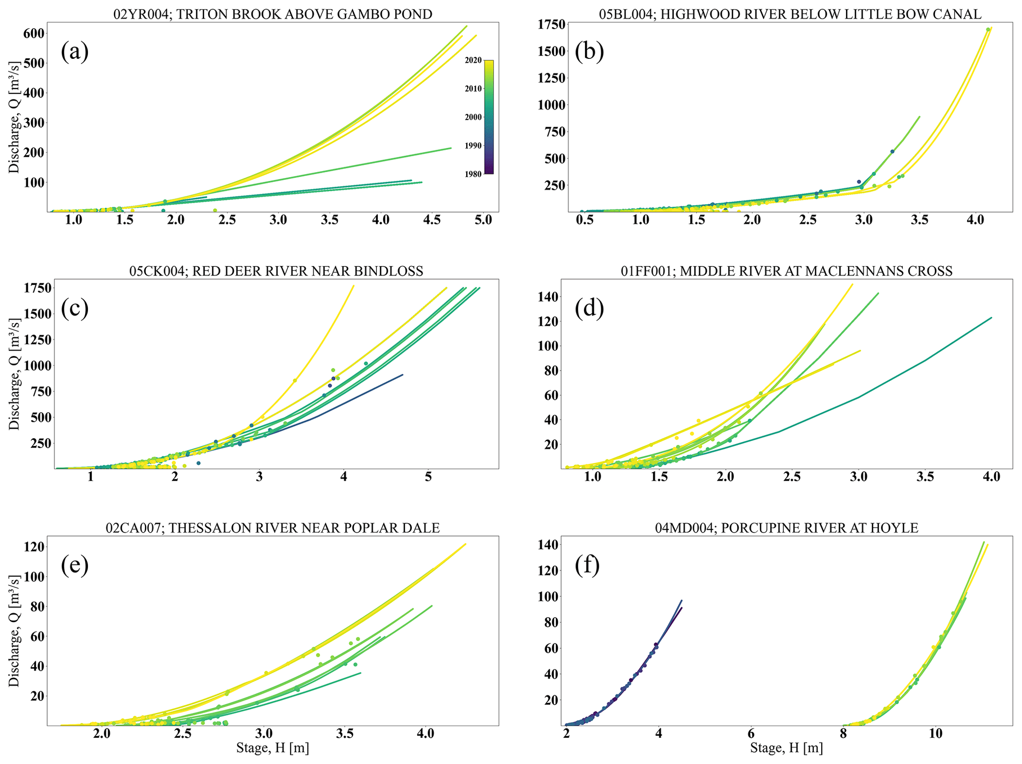
Figure 6 Examples of rating curves and observations available in Aquarius^™ illustrating rating curves over time: (a) curve extension outside of the highest discharge observation extrapolation; (b) sharp breaks in rating curves when the river flows out of bank; (c) under-ice stage–discharge observations not used in rating curve creation; (d) emphasis on one or a few stage–discharge measurements resulting in a change in the rating curve; (e) long- or short-term river bed erosion; and (f) change in the rating curve benchmark for reporting stage values.

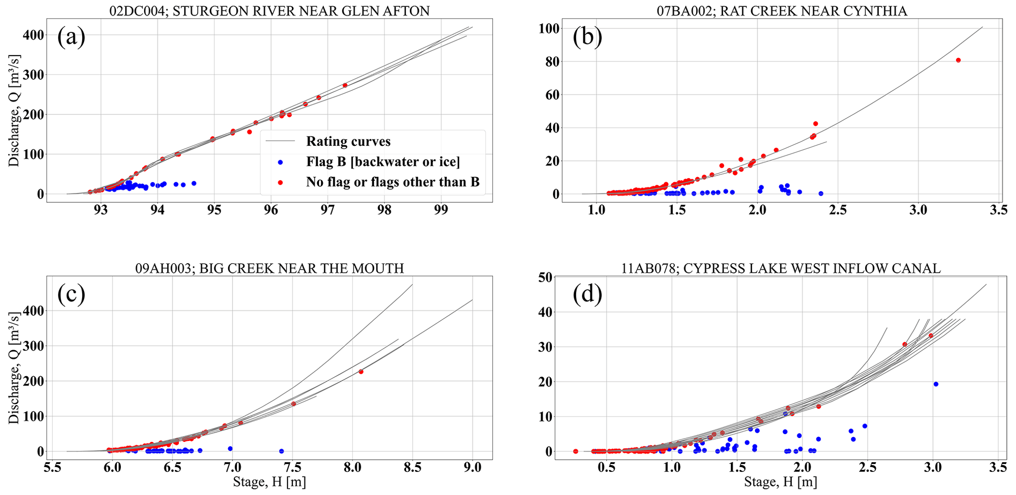
Figure 7 The contrast between the stage–discharge measurements with and without the B flag for stations (a) 2DC004, Sturgeon River near Glen Afton; (b) 07BA002, Rat Creek near Cynthia; (c) 09AH003, Big Creek near the mouth; and (d) 11AB078, Cypress Lake West Inflow Canal. The red points do not have flags, while the blue points are stage–discharge measurements that have the B flag, ice, or backwater in the operational database.

• Rating curve extrapolation or extension beyond the largest stage–discharge measurement in the operational database record. The rating curves might be extended beyond the largest stage–discharge observed values in the operational database. The method for the extension of the rating curves is not provided through the API in the operational database. Earlier observational discharges that are not recorded in the operational database may be used in creating more recent rating curves, or the extrapolation is done using hydraulic modeling or other procedures. For example, the difference in the rating curves for station 02YR004 is perhaps due to extrapolation outside the range of maximum observation using SOPs. For earlier rating curves that use linear tables this extrapolation is linear, while for more recent rating curves expressed in the logarithmic table the extrapolation is done in logarithmic space (Fig. 6a).

• Extrapolation of a rating curve for out-of-bank conditions. One of the difficulties is to construct a rating curve for out-of-bank conditions with limited observational points under high water conditions (Fig. 6b).

• Removal of ice-conditioned stage–discharge measurements. The formation of an ice cover causes increased friction and generates a backwater effect where the water level has a different relationship with discharge than under open-water conditions. Under a winter ice cover, discharges are much lower than during open water and measurements often do not fall on the stage–discharge curve. Instead, while ice is present, the observations are used to adjust the estimated discharges using overrides or temporary shifts (Fig. 6c). This, in turn, results in fewer observational points being available for the construction of rating curves.

• Emphasis on one or a few stage–discharge measurements. A rating curve is often created or changed based on one or a few stage–discharge measurements. Observational points with very high discharge values can affect the higher end of the rating curve. This can be due to high discharge values only occurring for brief periods, resulting in an observation in the high discharge period being the only one. In the example provided for station 01FF001, an observational point with a stage and discharge of approximately 1.75 m and 40 m³ s⁻¹ is given very high weight in creating the immediate rating curve update after the aforementioned field activity, while in later rating curves this high emphasis is not followed (Fig. 6d).

• Event-based erosion, flood, or long-term channel erosion. River sectioning may change over time, and therefore observational stage and discharge points follow these changes accordingly. Sediment transport occurs gradually and over periods longer than a flood event but can result in complex changes in the measurement section as sediment is deposited or removed or as dunes proceed through the section. These changes require a new rating curve or shifts in the existing rating curve (Fig. 6e). Similarly, floods or high water levels can also result in a substantial change in river sectioning or removal of stations. In these cases, a new rating curve is needed.

• Changes in the rating curve benchmarking stage or the instrument reading stage. A benchmark is a fixed point that is used to link the observed water level to an actual elevation. The local benchmark that is used as a datum may change over time with the landscape or administrative change. Alternatively, instrument replacement in a new location after a flood event, for example, can also change the readings to historical ones compared to the benchmark (Fig. 6f).

Given the above, it is important to emphasize that the use of rating curves within WSC does not allow for a more classical statistical approach for uncertainty analysis where the curve would be the best fit through the series of observed points (as it is for other institutions, such as the UK's Environment Agency; Lamb et al., 2003). The actual process used is deterministic, and much effort is invested in making the rating curve pass through or close to each measurement or stage and discharge point, which has been a long-standing practical approach (Rantz, 1982).

Seasonality and ice conditions are other factors that can complicate the use of existing stage–discharge observations. When there is ice cover, the stage–discharge relationship will differ substantially from the expected open-water rating curves. Figure 7 indicates that the stage–discharge measurements during cold months of the year were identified by flag B or backwater due to ice, in contrast to those with other or no flags. As is clear from the panels of Fig. 7, the winter period often has smaller discharge values for a similar stage than those in summer, thereby resulting in a smaller pool of stage–discharge observations that could be used for rating curve creation. Additionally, the presence of ice, similar to sedimentation, can result in the river bank and morphology changing over time and during an ice jam event, which may in turn result in a change in the rating curve over time (similar to Fig. 6c). This process of shaping the river morphology is hypothesized by Smith (1979) to result in less frequent bankfull events, which in turn results in less frequent peak flow measurement. The importance of river ice processes and their impact on stage and discharge values is reflected in the Canadian River Ice Database (CRID; de Rham et al., 2020).

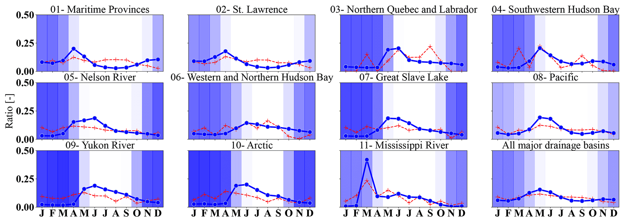
Figure 8 The lines indicate the monthly fraction of annual discharge in blue and stage–discharge measurements in red, for each major drainage basin and all the stations in the WSC operational database. The blue shading identifies the fraction of time series that are identified by flag B or backwater that is used to identify ice conditions. The darker the shade, the more dominant flag B or ice cover is for the major drainage basin.

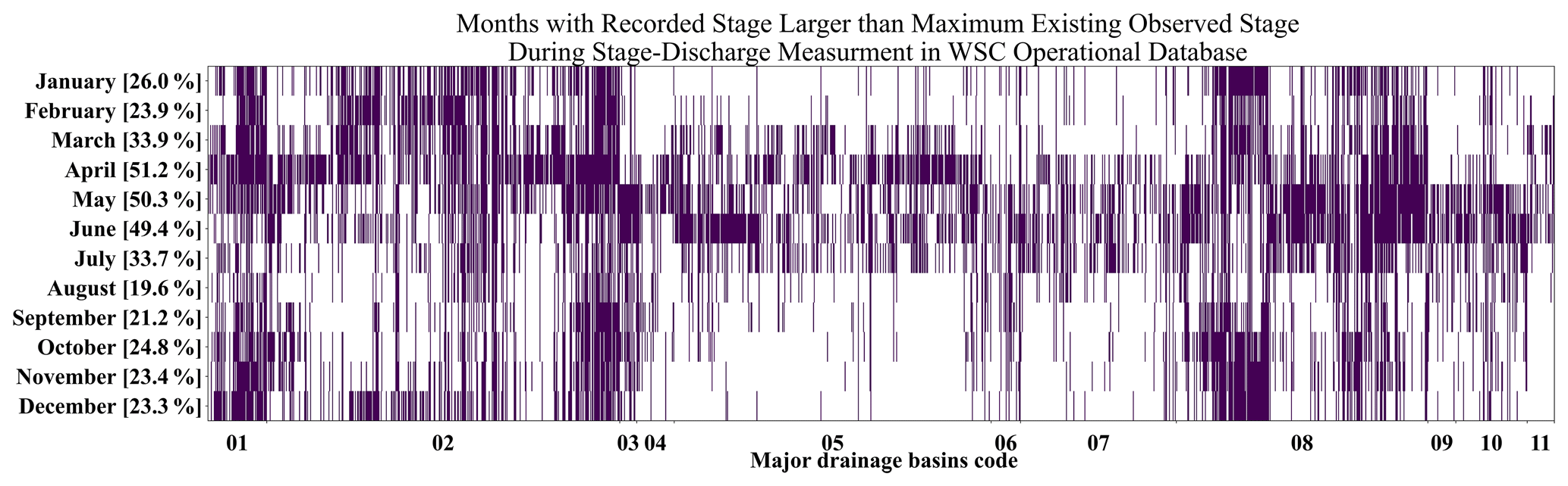
Figure 9 Months where the recorded stage values exceed the maximum observed stage during any discharge measurements archived in the operational database. A solid bar in a month in the figure indicates, for a station and during its available record, that there is at least one event in that month across all years, with recorded stage values exceeding the maximum observed stage value. The percentage for each month indicates the fraction of stations where the recorded stage exceeds the maximum observed stage and discharge.

Additionally, Fig. 8 provides fractions of discharge measurement activities, monthly fraction of annual discharge, and ice flags for each specific month of the year for the entire hydrometric network and 11 major drainage basins in Canada. The red dashed line indicates the change over the year for the percent of each month's in situ discharge measurements from the total number of discharge measurements, while the blue line provides an understanding of the magnitudes of the discharge values over the month of a year. The shaded blue for each month provides the comparison between the fraction of time in which the station time series for that month are identified by flag B (which is used to identify backwaters due to ice conditions). The number of discharge field measurement activities during the summer months is larger than in the winter months. This is due to the spring and summer variabilities in discharge being much greater than in winter and ice discharge measurements being expensive and labor-intensive in comparison to open-water measurements.

Evaluating the recorded stage as being greater than the maximum observed stage in the operational database provides an understanding of how often discharge estimates are in the parts of extrapolated rating curves beyond the observed stage–discharge points that are archived in the operational database. Figure 9 indicates that there are stations in which the stage higher than the maximum observed stage during discharge measurement can occur in any month of the year. One example of this is 02YR004, Triton Brook above Gambo Pond in the province of Newfoundland and Labrador (Fig. 6a). This could happen because the operational database might not include earlier stage–discharge measurements with the highest stage values or systematic backwater from increased water levels in Gambo Pond. In general, Fig. 9 highlights the existence of numerous events when discharge values are estimated using extrapolated segments, which can have significant impacts on estimates of discharge and its uncertainty in flood modeling and flood forecasting.

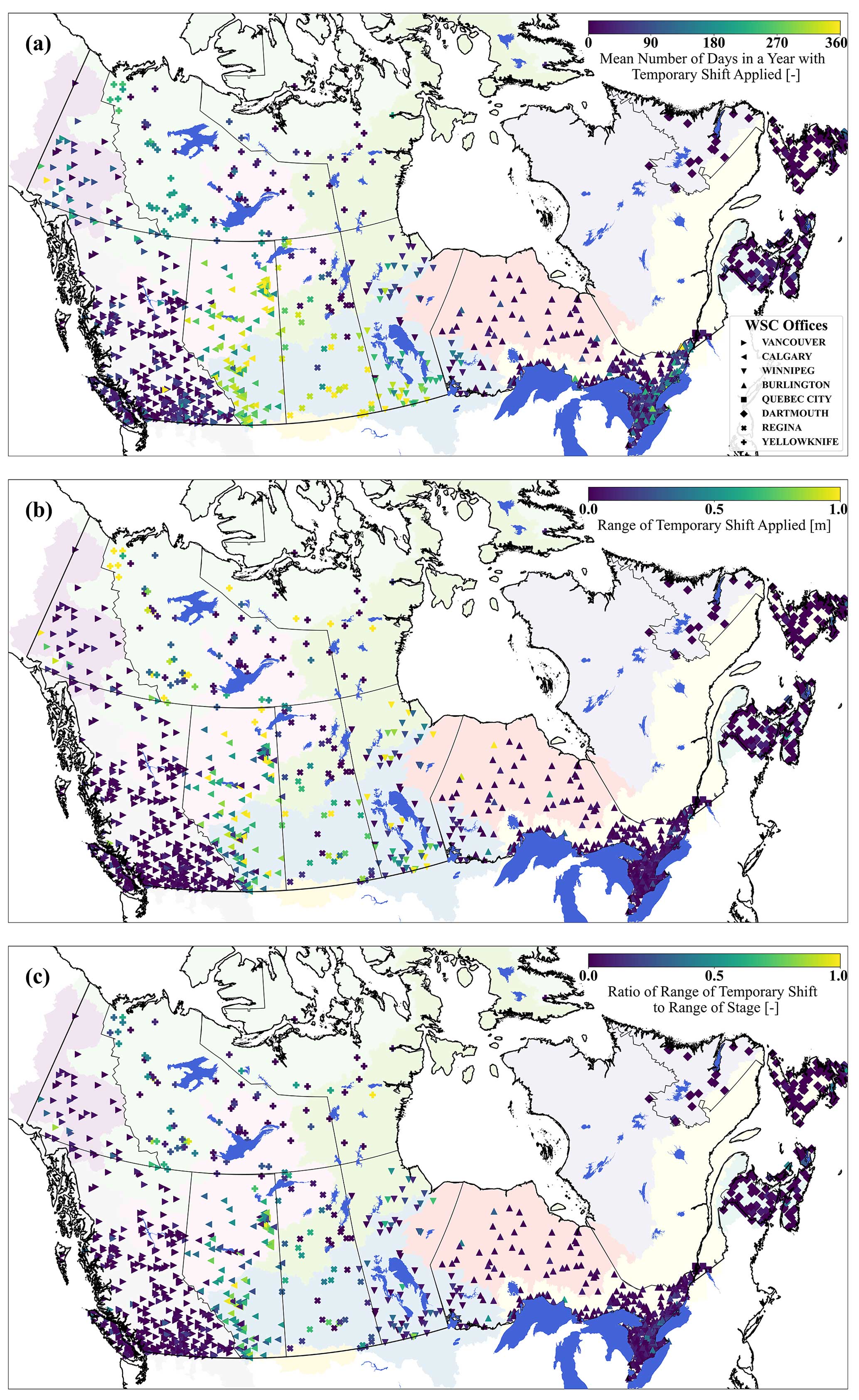
Figure 10 (a) Temporal application of temporary shift, (b) range of applied temporary shift, and (c) ratio of the temporary shift range to the stage range across hydrometric stations of WSC. The background colors indicate the major drainage basins (see Fig. 1). The analysis is limited to stations and their time series that cover at least 360 d yr⁻¹ (non-seasonal), resulting in the ∼ 1340 stations shown in this figure.

The temporary shift in the rating curves to account for environmental conditions is a common practice at the regional offices of WSC. Figure 10 identifies three major characteristics of temporary shift application across Canadian hydrometric stations. First is the average number of days per year on which temporary shift is applied (Fig. 10a). For the Prairie region, especially for stations operated by the Calgary office in the province of Alberta, the temporary shift can be applied all year long (length of temporary shift application larger than 300 d yr⁻¹). As presented in Fig. 10, using the temporary shift to adjust for environmental conditions is most common in the Prairie and Northern regions. The use of temporary shifts is less common in eastern and western Canada. In those regions, direct manipulation of discharge values rather than the rating curves is more common (following override). The second panel, Fig. 10b, indicates the magnitude of the temporary shift applied in meters. There are stations with a temporary shift magnitude of more than 1 m; this means that, during various environmental conditions such as the presence of thick ice cover, stage values that are as different as 1 m or more under the temporary shift application may result in similar discharge estimation. Lastly, Fig. 10c identified the range of the applied temporary shift to the range of stage values. This comparison indicates how relative intervention by temporary shift is compared to changes in the recorded stage values. Interestingly, there are stations over the Canadian domain in which the range of temporary shift surpasses the range of recorded stage values (ratio of close to or more than 1).

3.2 Time series reconstruction

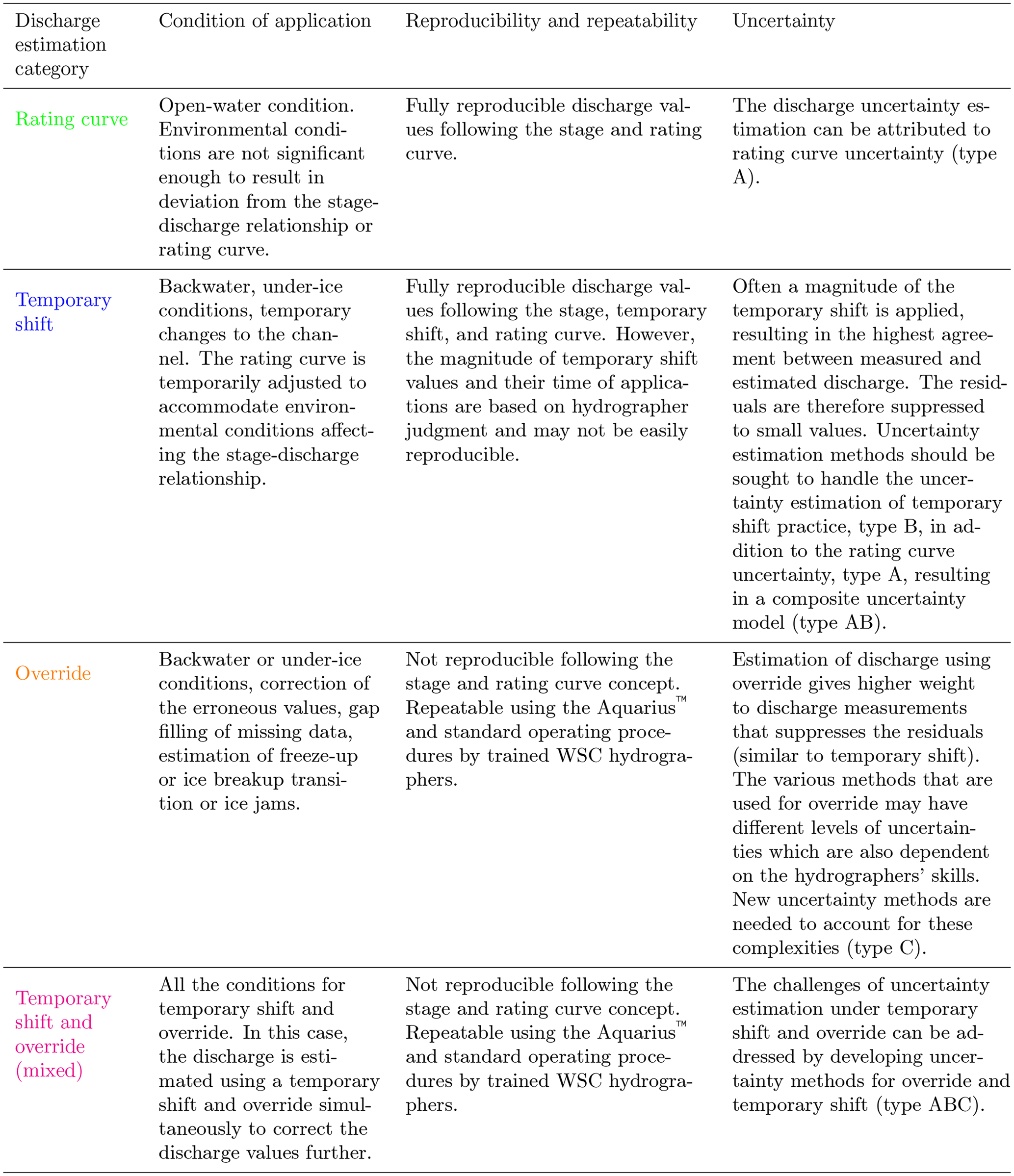
In steps 3 and 4 of the independent workflow, river discharge values are reconstructed and compared with the reported discharge values from the WSC operational database. This comparison of discharge values indicates four categories for discharge estimation:

1. Rating curve. The estimated discharge values strictly follow the stage–discharge relationship or rating curves and can be reconstructed using recorded stage time series.

2. Temporary shift. The discharge follows the temporarily shifted rating curves and can be reconstructed using stage time series.

3. Override. The period in which the discharge is estimated using override methods and techniques (not following the rating curve and temporary shift).

4. Temporary shift and override. Both temporary shift of the rating curve and the override method are applied at the same time to estimate discharge values.

Table 1 indicates the four categories of discharge estimation and their reproducibility using the independent Python workflow, given the data that were retrievable from the API system.

Table 1 Types of discharge estimation; the colors correspond to Figs. 11 to 15.

To provide clear examples of each of the categories, four stations are examined. Figure 11a illustrates the recorded stage for 08GA079 (Seymour River above Lakehead) located in the province of British Columbia. The applied temporary shift and the dates of field or discharge measurements are shown in panel (b). Panel (c) compares the recreated discharge using the workflow described in this study and the reported discharge from the operational database. The shaded areas in this panel indicate the quality assessment symbol (flag) from the operational dataset. There is no application of temporary shift and override for this station in the year 2002, and therefore the estimated discharge follows the rating curve concept (shown in green in panel d).

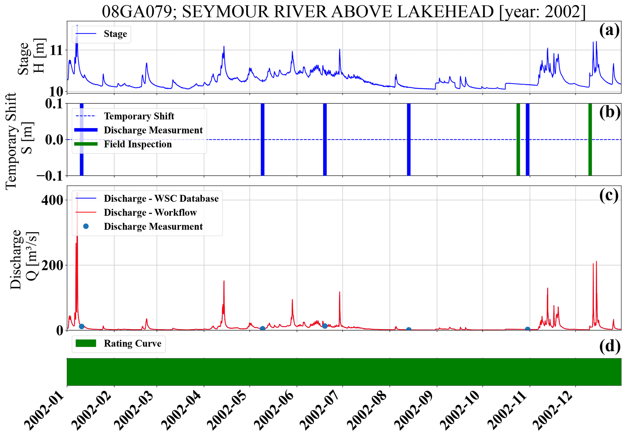
Figure 11 (a) The recorded stage, (b) the applied temporary shift, (c) reproduced discharge values based on workflow and comparison to reported discharge values from operational database and discharge measurements, and (d) the dominant method of discharge estimation for 08GA079 (Seymour River above Lakehead) in the province of British Columbia. The colors in the lower bar link to the descriptions in Table-1: rating curve (green).

Figure 12 illustrates the stage, temporary shift, and reported and reconstructed discharge values and time series for station 01AF009 (Iroquois River at Moulin Morneault) located in the province of New Brunswick. The under-ice condition in the reported discharge values from the operational database is lower than the reconstructed discharge values from the stage using the rating curves and temporary shift of zero values, while the applied temporary shift values for the year 2003 are zero. The under-ice discharge estimate is an override applied using various methods at the regional offices. It can be seen that override discharge values pass through the observational points under ice conditions, that these observations of discharge are the basis for the winter flow record and not the recorded stage and rating curves, and that the variation is recreated following the established logic at the regional office, such as under-ice peak flows (late March and early April in this example). This is reflected in panel (d), in which two major discharge estimation categories are depicted: green is where rating curves are followed without temporary shift, and gold is where the override methods are applied.

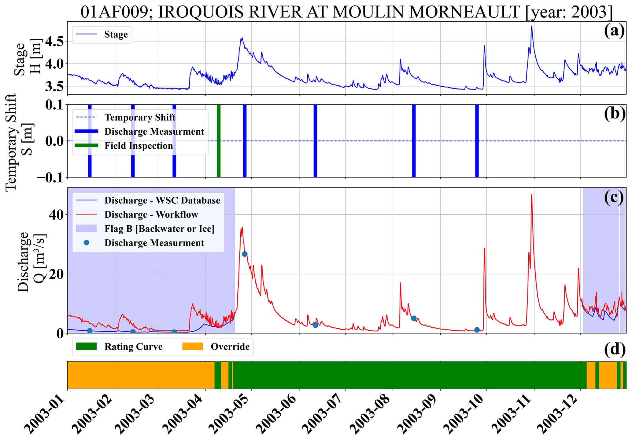
Figure 12 (a) The recorded stage, (b) the applied temporary shift, (c) reproduced discharge values based on workflow and comparison to reported discharge values from operational database and discharge measurements, and (d) the dominant method of discharge estimation for 01AF009 (Iroquois River at Moulin Morneault) located in the province of New Brunswick. The colors in the lower bar link to the descriptions in Table-1: rating curve (green) and override (gold).

Discharge values for station 05BL004 (Highwood River below Little Bow Canal) are provided in Fig. 13. The hydrographers have applied negative temporary shifts for this station. For the year 2012, the temporary shift was applied during winter with larger values (−0.25 to −0.50) and during summer with rather smaller values ($<-\mathrm{0.20}$). The winter temporary shift is presumed to be correcting for ice conditions, and the summer temporary shift, in June, is likely for the backwater correction over the high discharge period (while there is no flag associated with this event). Temporary shifts are sometimes applied on dates that coincide with discharge measurements or site visits, presumably to match the observed discharge with the rating curve with temporary shifts. Temporary shift values can be changed on other dates that might correspond to temperature changes or video recordings from on-site monitoring cameras or upstream and downstream station field visits and observations. Panel (d) indicates that, for this station and the year of interest, there are two major discharge estimation categories: blue is the rating curve and temporary shift, and magenta is the rating curve and the temporary shift which is corrected by override.

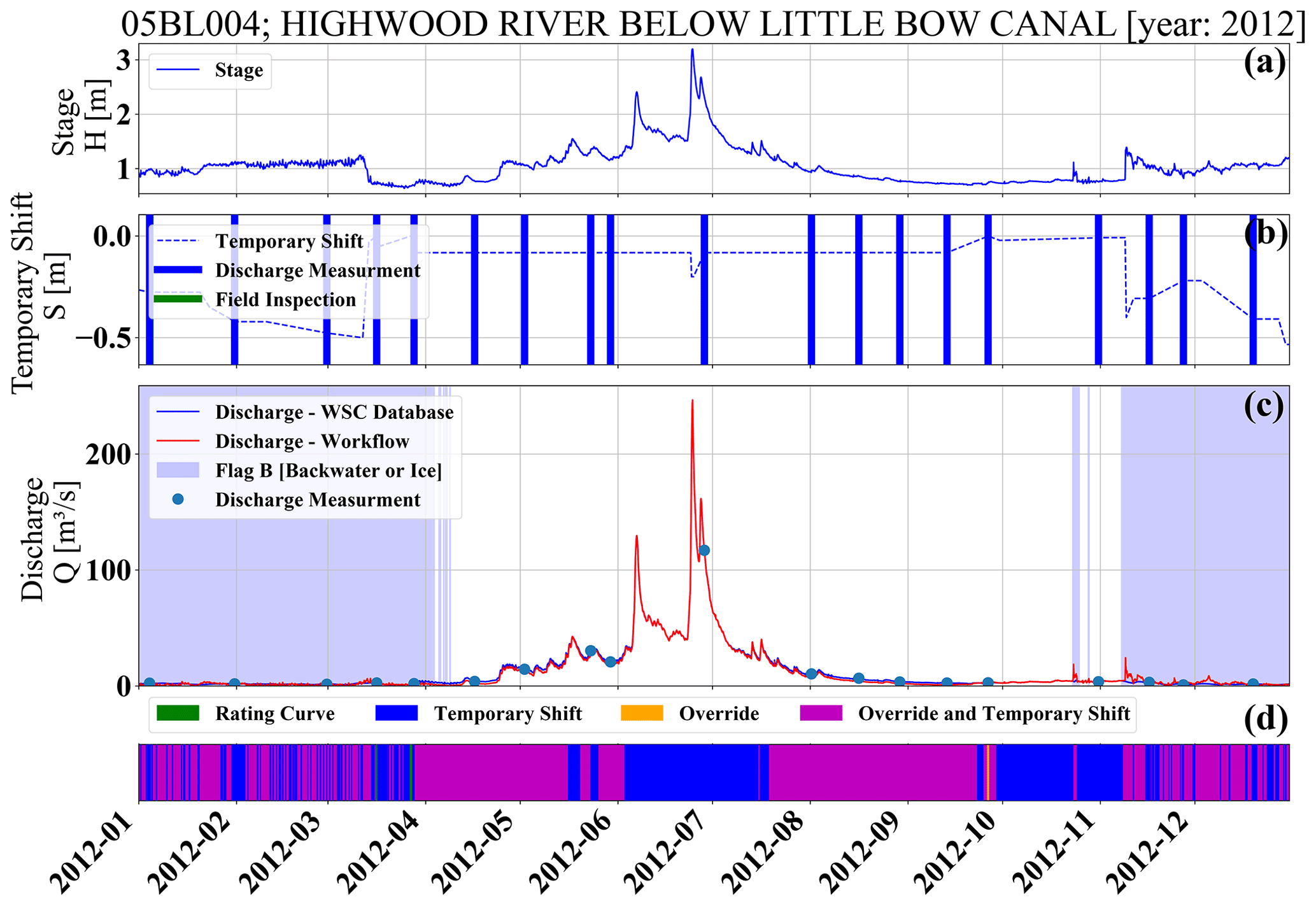
Figure 13 (a) The recorded stage, (b) the applied temporary shift, (c) reproduced discharge values based on workflow and comparison to reported discharge values from operational database and discharge measurements, and (d) the dominant method of discharge estimation for 05BL004 (Highwood River below Little Bow Canal) located in the province of Alberta. The colors in the lower bar link to the descriptions in Table-1: rating curve (green), temporary shift (blue), and override with temporary shift and override (magenta).

The last example focuses on station 09CB001, White River at Kilometer 1881.6 Alaska Highway in Yukon Territory (Fig. 14). This is an example of a station in which a variety of discharge estimation methods are used. In part of the summer, the discharge can be fully reproduced by rating curves. There are also periods in which the temporary shift is applied over summer and discharge estimation follows the rating curve and temporary shift. In part of the summer, in addition to the temporary shift concept, override is also applied to correct the estimated discharge. For the winter period, there is no application of temporary shift. However, override is used by emphasizing the observation, perhaps under ice observation, to estimate discharge (similar to Fig. 13).

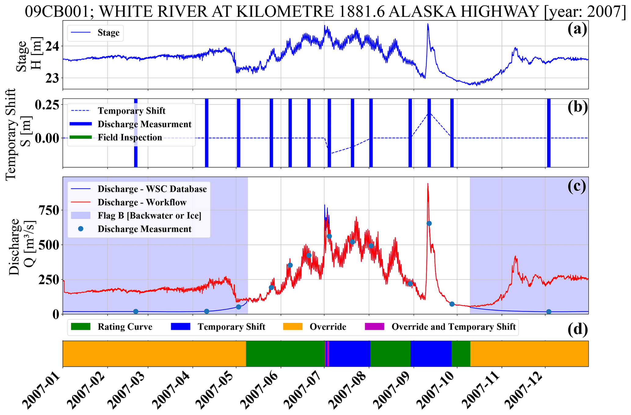
Figure 14 (a) The recorded stage, (b) the applied temporary shift, (c) reproduced discharge values based on workflow and comparison to reported discharge values from operational database and discharge measurements, and (d) the dominant method of discharge estimation for 09CB001 (White River at Kilometer 1881.6 Alaska Highway in Yukon Territory). The colors in the lower bar link to the descriptions in Table-1: rating curve (green), override (gold), temporary shift (blue), and override with temporary shift and override (magenta).

Given the difference between the reproduced and reported discharge values in the operational database, similar to station 01AF009, in the following the agreement between the reported discharge in the operational database is evaluated using the independent workflow for all the hydrometric stations that have a complete yearly record. Figure 15a illustrates the overall categories for discharge estimation for stations with complete yearly discharge values (not seasonal). For example, as expected, this panel shows that the rating curve category is more dominant in regions of the Maritime Provinces and St. Lawrence basins during the summer period, followed by override categories that are mostly applied in winter. In contrast, for Saskatchewan and the Nelson River, the temporary shift is more dominant in wintertime together with a mixture of temporary shift and override. The estimation of discharge values with an independent workflow can be compared with the reported discharge in the operational database. Figure 15b depicts this agreement in a fraction of the period in which reconstructed discharge is within 5 % of the discharge reported in the operational database. The overall overlap is around 0.69. This level of agreement from the independent workflow can be attributed to discharge estimation from rating curves and rating curves combined with the temporary shift. On the other hand, the lack of agreement can be heavily attributed to the override values, which are more pronounced during the winter period. This lack of agreement can be partly attributed to the types of data that are not available from the WSC operational database via the API (which is used for the workflow in this study). Trained and experienced WSC hydrographers can repeat discharge values, with great if not identical similarities, using the Aquarius^™ documented comments in the operational database. This is also checked and confirmed during the approval process. Therefore, the repeatability, in practice, will be much higher than the reproducibility reported based on the independent workflow stated here.

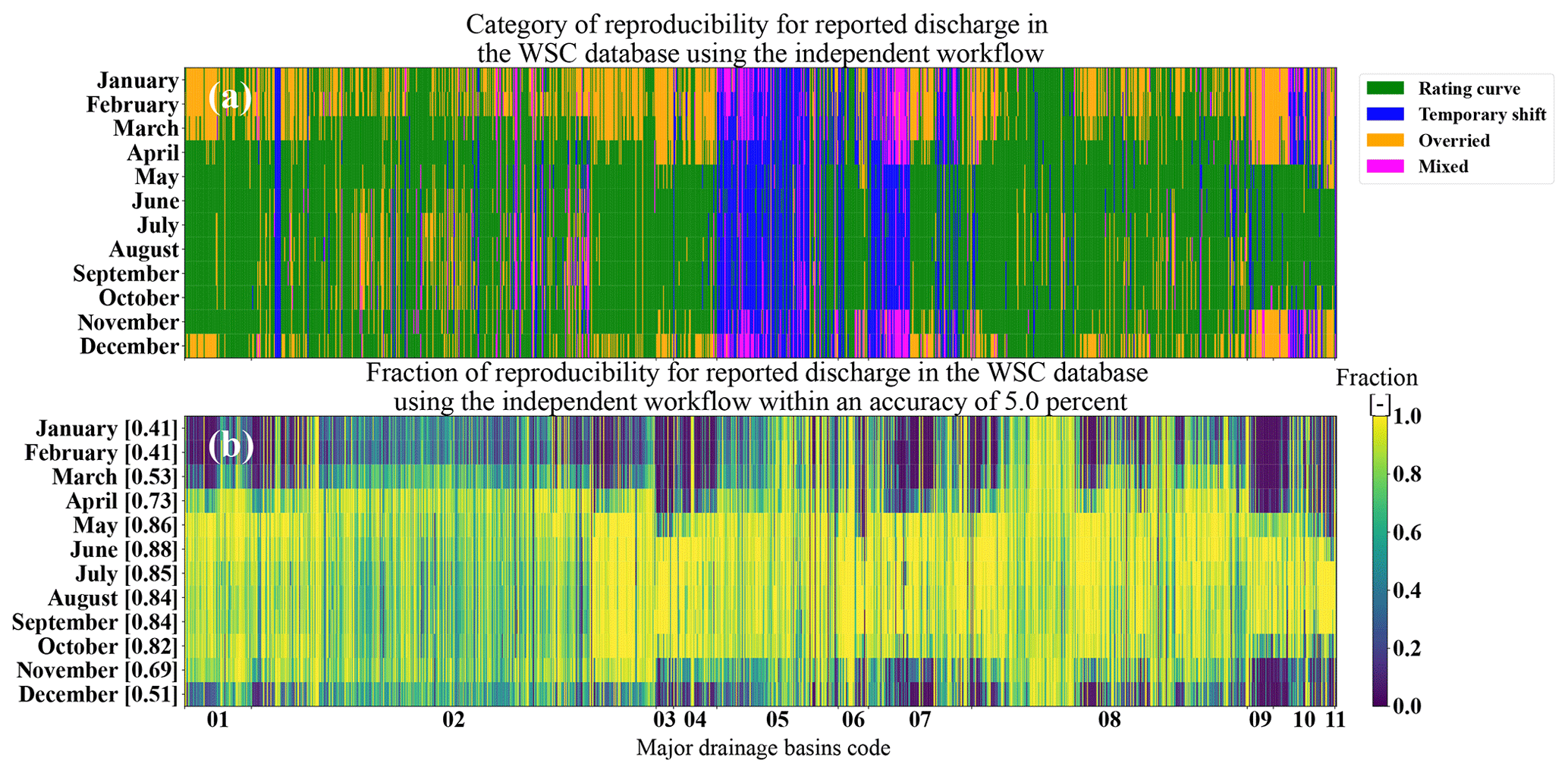
Figure 15 (a) The dominant category of discharge estimation over month of the year; these categories are (1) the rating curve on which the discharge estimation fully follows the concept of a rating curve, (2) temporary shift when the discharge estimation conforms to the concept of a temporarily shifted rating curve, (3) override when the discharge is altered outside of the concept of a (temporarily shifted) rating curve, and (4) mixed categories in which a combination of temporary shift and override is used. (b) The fraction of agreement for estimated discharge values from the proposed workflow described in this study (within 5 % of reported discharge values from the WSC operational database). The agreement fraction is not always at its maximum, 1.00, and varies seasonally and geographically. The overall average agreement between the recreated discharge values and what is reported in the operational database is 0.69, with the winter months having lower agreement than the summer months. The analysis is limited to stations and their time series that cover at least 360 d yr⁻¹ (non-seasonal), resulting in the ∼ 1340 stations shown in this figure.

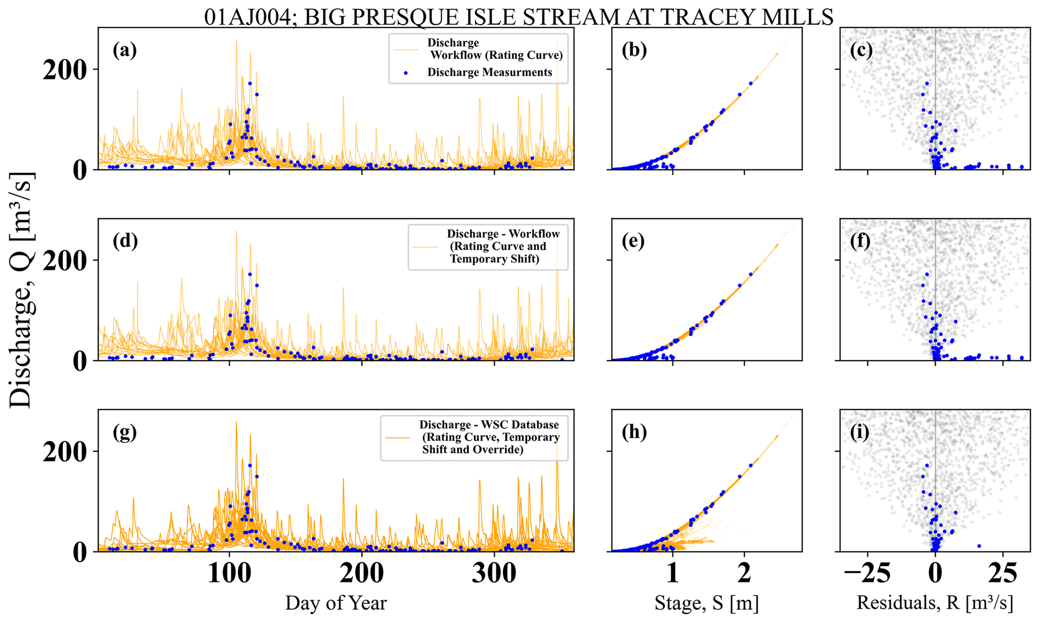
Figure 16 The comparison between discharge values for estimated discharge for each day of the model, stage–discharge relationships, and residuals for three difference cases for station 01AJ004 (Big Presque Isle Stream at Tracey Mills) located in the province of New Brunswick: (a–c) when the discharge estimation strictly follows the rating curve, (d–f) when the discharge estimation follows both the rating curve and the temporary shift, and (g–i) for the WSC operational database that includes the rating curve, temporary shift, and override. In contrast, the grey dots are the hypothetical case of the normal distribution with a heteroscedastic standard deviation of 10 % of the discharge magnitude.

3.3 Implication for uncertainty estimation

The processes of temporary shift and override affect the residual values that are the foundation of uncertainty estimation models. In this section, we examine how different discharge estimation methods, such as the rating curve, temporary shift, and override, alter the stage–discharge relationship and subsequently the residuals.

Figure 16a depicts the discharge time series based on the rating curve for station 01AJ004, Big Presque Isle Stream at Tracey Mills, New Brunswick, for each day of the year alongside the discharge measurements. Figure 16b illustrates the stage–discharge relationship compared to the discharge measurement values. Due to the strict adherence to the rating curve, the stage–discharge space is confined to the rating curves only. Figure 16c depicts the residuals for each discharge measurement compared to the estimated discharge from the workflow following the rating curves only (no temporary shift or override). The grey background points represent a hypothetical case of residuals with a normal distribution of 10 % of discharge magnitude heteroscedasticity. Station 01AJ004 is in the region where override is more commonly used for discharge estimation than temporary shift. Thus, Fig. 16d–f, which are based on discharge estimation using the rating curve and temporary shift, closely resemble Fig. 16a–c (indicating that no major temporary shift is applied). The same analysis was repeated using the discharge reported by the WSC operation database, which includes override processes. As shown, the override results in lower discharge values during the colder months of the year in Fig. 16g compared to Fig. 16a and d. This reduction leads to closer agreement between the reported discharge time series and the discharge measurements. Additionally, Fig. 16h indicates that, due to the override intervention, the stage–discharge relationship is no longer restricted to the rating curve. The winter streamflow override corrections minimize the residuals between the discharge measurements and the reported values, as seen in Fig. 16i, compared to Fig. 16c and f.

As the next example, we examine station 05CK004, Red Deer River near Bindloss, located in Alberta. This station is managed by the Calgary office, where the temporary shift is more prevalent than the override in discharge estimation processes. The contrast between Fig. 17a and d highlights the impact of the temporary shift on the estimated discharge, especially during the colder months or under ice conditions. This use of the temporary shift causes the stage–discharge space depicted in Fig. 17e to extend beyond the rating curve and pass through the observational points shown as blue dots, indicating a higher emphasis on discharge measurement values. Similarly, the residuals for low-flow or ice conditions are minimized in Fig. 17f compared to Fig. 17c. In addition to the temporary shift, override processes further reduce the residuals, as shown in Fig. 17i, in contrast to Fig. 17c and f.

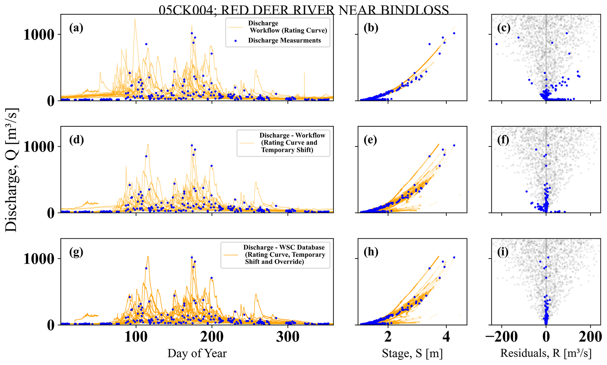
Figure 17 The comparison between discharge values for estimated discharge for each day of the model, stage–discharge relationships, and residuals for three difference cases for station 05CK004 (Red Deer River near Bindloss) located in the province of Alberta: (a–c) when the discharge estimation strictly follows the rating curve, (d–f) when the discharge estimation follows both the rating curve and temporary shift, and (g–i) for the WSC operational database that includes the rating curve, temporary shift, and override. In contrast, the grey dots are the hypothetical case of the normal distribution with a heteroscedastic standard deviation of 10 % of the discharge magnitude.

4 Discussion

This work presents discharge estimation methods used by WSC following an independent Python workflow. The study explores the SOPs for creating rating curves, manipulating them over time, and estimating discharge. The study focuses on two major discharge estimation SOPs, i.e., temporary shift and override. The impact of these SOPs on discharge estimation and uncertainty evaluation, specifically in terms of residuals, is discussed. By examining the SOPs and their possible impact on discharge estimation and the associated uncertainties, the study aims to highlight the need for new discharge uncertainty methods.

The relationship between the rating curves and observational stage–discharge measurements is explored. The WSC SOPs differ from more commonly used practices in other parts of the world (McMillan et al., 2010; Coxon et al., 2015), largely due to the hydrological regimes and conditions faced by WSC in Canada. Temporary shifts and override processes, while giving the observational stage–discharge a high weight in discharge estimation, result in a more complex relationship between the rating curve and observations than a standard curve-fitting exercise (Figs. 16 and 17). This complexity does not lend itself well to more traditional uncertainty approaches. New methods must be explored to evaluate the rating curve uncertainties over and above the already existing methods that rely on the specific nature of residuals, such as heteroscedastic Gaussian, in the literature. For example, the methods suggested or applied by Clarke (1999), Jalbert et al. (2011), Le Coz et al. (2014), and Kiang et al. (2018) are not readily applicable to Canadian hydrometric realities.

Following the available information in the WSC operational database accessible by the API and the independent Python workflow, the agreement level between the two discharge estimations, from the workflow and operational database, is explored. This agreement is significantly lower during the colder months, which in turn indicates the complication of the discharge estimation under ice conditions and their backwater effect. To account for this environmental factor, different regional offices may follow different procedures rather than rating curves. In parts of Canada, the override procedure is used, while the Prairie and Northern regions rely heavily on the temporary shift of rating curves (Fig. 10).

This work provides the basis for future uncertainty analysis of discharge values reported by WSC. For better estimation of discharge values as an outside user together with the associated uncertainties, however, more information needs to be added to the WSC operational database and more capabilities need to be developed for the Aquarius^™ system. This information does exist in WSC offices on paper, in field notes, and on local computer systems but is not fully transferable to the operational database. As an example, during the preparation of this work and from the API system, it was not possible to find out which observational stage–discharge points were used for rating curve creation by hydrographers. Additionally, the information that might help with observational stage–discharge uncertainty was not available through the API to the best of the authors' knowledge. The inclusion of the rationale behind the magnitude and date of application of the temporary shift or override methods can be a great asset for the operational database. This reflects the concepts of repeatability and reproducibility. A trained hydrographer at WSC can repeat, based on SOPs, the work and decisions of other colleagues with a high degree of repeatability. As mentioned earlier, this is a routine practice for quality assurance. However, a fully reproducible workflow based on an agreed-upon model is missing, which is essential for the uncertainty analysis of discharge values. This is critical in trend analysis for separating the impact of discharge estimation processes and natural variability over time (see Figs. 5 and 6 of Hamilton and Moore, 2012). The recommendations transcend the WSC operational procedures and agencies that follow similar approaches to WSC. As an example, WSC and the United States Geological Survey, USGS, have a long history of collaboration going back to the beginning of the WSC's mandate in 1908. The chief hydrographer of Canada spent his early years training with USGS staff in Montana, and since then both organizations have developed shared common practices. Both the USGS and WSC use Aquarius^™ as their primary data production platform, and the practices of override and temporary shift are used by the two organizations. Additional effort is still needed to assess the similarities and implications of procedural practices for discharge estimation and uncertainty quantification between the two countries.

From a broader perspective, this study, given the complexity of the production system and updates of the rating curve information, encourages the community to consider the provenance of discharge data and evaluate their fitness for their intended use (Whitfield, 2012). The discharge values are more than just a true or deterministic value disseminated from the HYDAT dataset by WSC. This dataset is often used in large-sample hydrology (Gupta et al., 2014) and is carried over to the larger datasets without its error and uncertainties being communicated. For example, datasets from Addor et al. (2017), Arsenault et al. (2020), and Kratzert et al. (2023) do not include discharge uncertainty values. These discharge values are then used for scientific purposes, model development, and model intercomparison alongside recently used machine learning techniques. If uncertainty and errors in discharge are ignored, the use of large-sample datasets may result in misleading or strong conclusions. For example, it has been communicated that machine learning can predict discharge values with 99 % accuracy or can predict discharge superior to traditionally used mechanistic Earth system models (in the literature or in blog posts). These comments and conclusions should be regarded with caution as hydrographers' decisions in estimating discharge can significantly change a hydrograph (shown in Figs. 5 and 6 of Hamilton and Moore, 2012). Instead, efforts should be focused on reassessing those claims with an ensemble of discharge values. Using an ensemble of discharge time series alongside an ensemble of forcing variables of precipitation and temperature can provide a much more robust analysis of scientific methods, decisions, and claims for Earth system models (Cornes et al., 2018; Wong et al., 2021; Tang et al., 2022).

5 Conclusions

We summarize our major findings as follows:

• The Water Survey of Canada's standard operating procedures in estimating discharge from stage values, particularly temporary shift and override, are explored and explained by an independent Python workflow.

• There is no single approach for estimating the rating curve from past observational (stage and discharge) points at the Water Survey of Canada. This is perhaps due to the complex relationship between stage and discharge, accounting for the complexity and diversity of discharge values over the range of environmental conditions for Canadian hydrometric stations. Additionally, given SOPs such as override and temporary shift, relationships between rating curves and observational stage–discharge points are more complex than just a curve-fitting exercise.

• Given the knowledge of discharge estimation processes, the reported discharge values in Aquarius^™ can be reproduced for a fraction of 0.69 (within 5 % accuracy). The other 0.31 non-reproducible fraction can be heavily attributed to the override. The reader should note that the reproducibility statistic is based on the independent Python workflow provided in this study and the reproducibility of the discharge estimation methods to the extent possible. However, repeatability by trained and experienced WSC hydrographers may result in a much higher level of agreement than what is presented in this work.

• The standard operating procedures, or SOPs, of temporary shift and override result in the residuals being suppressed to minimal values. These will not follow the often-assumed statistical distributions for residuals or the fundamental basis for rating curve uncertainty estimation methods. Additional uncertainty models for rating curves that do not have structured residuals in comparison to stage and discharge measurements, temporary shift, and override techniques should be constructed and evaluated for Canadian hydrometric stations (uncertainty models of types A, AB, C, and ABC from Table 1).

Finally, we encourage knowledge mobilization and further collaboration between WSC, the private sector, and universities and research institutes, similar to this work, which will open up opportunities for the evaluation of organizational processes and constant improvement and stimulate the need for science improvement.

Appendix A: General terms and their descriptions

Table A1 General terms and their descriptions.