FROSTBYTE: a reproducible data-driven workflow for probabilistic seasonal streamflow forecasting in snow-fed river basins across North America

Seasonal streamflow forecasts provide key information for decision-making in fields such as water supply management, hydropower generation, and irrigation scheduling. The predictability of streamflow on seasonal timescales relies heavily on initial hydrological conditions, such as the presence of snow and the availability of soil moisture. In high-latitude and high-altitude headwater basins in North America, snowmelt serves as the primary source of runoff generation. This study presents and evaluates a data-driven workflow for probabilistic seasonal streamflow forecasting in snow-fed river basins across North America (Canada and the USA). The workflow employs snow water equivalent (SWE) measurements as predictors and streamflow observations as predictands. Gap-filling of SWE datasets is accomplished using quantile mapping from neighboring SWE and precipitation stations, and principal component analysis is used to identify independent predictor components. These components are then utilized in a regression model to generate ensemble hindcasts of streamflow volumes for 75 nival basins with limited regulation from 1979 to 2021, encompassing diverse geographies and climates. Using a hindcast evaluation approach that is user-oriented provides key insights for snow-monitoring experts, forecasters, decision-makers, and workflow developers. The analysis presented here unveils a wide spectrum of predictability and offers a glimpse into potential future changes in predictability. Late-season snowpack emerges as a key factor in predicting spring and summer volumes, while high precipitation during the target period presents challenges to forecast skill and streamflow predictability. Notably, we can predict lower-than-normal and higher-than-normal streamflows during spring to early summer with lead times of up to 5 months in some basins. Our workflow is available on GitHub as a collection of Jupyter Notebooks, facilitating broader applications in cold regions and contributing to the ongoing advancement of methodologies.

1 Introduction

Seasonal streamflow forecasts play an important role in various sectors, including water supply management, hydropower generation, and irrigation scheduling. They can also provide early warning of floods and droughts. Around the globe, a diverse range of predictors play a crucial role in seasonal streamflow forecasting. This includes antecedent hydrological conditions (e.g., snowpack, past streamflow, soil moisture) and future conditions (e.g., future precipitation, climate signals). See Yuan et al. (2015) for a comprehensive review of the dominant sources of seasonal hydrological predictability. Various forecasting methods leverage these predictors and hydrological processes that drive streamflow variability in regions of interest.

In Canada and much of the USA, snowmelt is an important driver of streamflow. In spring, the snow accumulated during winter serves as a substantial water reservoir in high-altitude mountainous regions, often referred to as “water towers” (Viviroli et al., 2007). Gradually, this natural water storage releases its stored contents downstream to the rivers through the process of snowmelt. In the western USA, operational seasonal hydrological forecasting relies on the long-term predictability provided by winter snow conditions (Wood et al., 2016). This important natural water supply is however threatened by climate change. Immerzeel et al. (2020) assessed the vulnerability of the world's water towers and found that, in North America, vulnerabilities are associated with both population growth and rising temperatures. By understanding the predictability of streamflow originating from snowmelt, we can better address the challenges posed by climate change and effectively manage these invaluable water sources for the future.

Over the past few decades, significant advances have been made in our understanding of forecast quality and hydrometeorological predictability on seasonal timescales. These have been facilitated, in part, by continuous improvements in technological capabilities. As a result, a wide range of approaches now exists for streamflow forecasting on seasonal timescales, including process-based, data-driven, and hybrid models, each possessing distinct advantages and limitations (Slater et al., 2023). This paper focuses on data-driven approaches.

Data-driven forecasting involves predicting a variable of interest (known as a predictand, e.g., streamflow spring volumes) by establishing relationships between the predictand and one or more predictors (e.g., snowpack, past streamflow, climate signals). Various techniques can be employed to model these relationships, ranging from simple linear regressions to more complex machine learning (ML) and/or artificial intelligence (AI) methods. Consider the following noteworthy data-driven approaches for seasonal streamflow forecasting: (i) principal component regressions (PCRs) have proven effective in streamflow volume forecasting in the USA (Garen, 1992; Mendoza et al., 2017; Fleming and Garen, 2022); (ii) Bayesian joint probability statistical modeling has demonstrated its capability in ensemble seasonal streamflow forecasting in Australia (Wang et al., 2009); (iii) seven different generalized additive models for location, scale, and shape statistical models were tested to forecast quantiles of seasonal streamflow in the US Midwest, using a range of predictors such as precipitation, temperature, agricultural land cover, and population (Slater and Villarini, 2017); (iv) a robust M-regression model was first tested for hydrological forecasting for ensemble seasonal streamflow forecasting in the South Saskatchewan River basin (Canada), extending the operational forecast lead time by up to 2 months (Gobena and Gan, 2009); (v) regression models were applied for winter and early spring streamflow forecasting in large North American river basins in Canada and the USA, based on snowpack information (Dyer, 2008); and (vi) ML or AI is now increasingly being explored for this type of application. Fleming et al. (2021) explored the use of AI for forecasting of water supplies in the western USA. They showed that it meets the quality and technical feasibility requirements for operational adoption at the US Department of Agriculture Natural Resources Conservation Service (NRCS).

This work builds on the literature and addresses research gaps by extending the spatial domains of previous studies to include both Canada and the USA. In this work, we use PCRs to predict future streamflow from snow water equivalent (SWE) information as the sole predictor given its importance for seasonal streamflow prediction. PCR stands as a well-established and widely used data-driven method, as demonstrated by the non-exhaustive list above. Simple statistical regression methods such as PCR offer several key advantages, including their local applicability, intuitive nature (i.e., use of local data to represent known and observed hydrological processes locally), speed, and low computational resource requirements. These methods are additionally straightforward to implement and potentially highly reliable.

Mendoza et al. (2017) showed that increasing methodological complexity (in their study this was defined as the gradient from purely data-driven techniques to the use of process-based models) does not always lead to improved forecasts. Emphasizing simplicity in modeling provides a robust foundation for enhancing our comprehension of hydrological processes and supports ongoing improvements to forecast quality (including through model developments and the use of new observations), as highlighted by Delgado-Ramos and Hervas-Gamez (2018). This approach additionally supports reproducibility to enable collaborative advancements through open-science practices (Knoben et al., 2022).

In this paper, we present a reproducible data-driven workflow designed for probabilistic streamflow forecasting in nival (i.e., snowmelt-driven) river basins across Canada and the USA (Sect. 2). For the sake of simplicity, we use the term “North America” to refer to the forecasting domain used in this study. Through the analysis of the hindcasts produced with this workflow, we address this research question: can SWE be used as a reliable predictor of future streamflow in nival river basins across North America (Sect. 3)? In the discussion of our findings, we extract essential insights relevant to snow-monitoring experts, forecasters, decision-makers, and workflow developers, addressing an important research gap in knowledge translation (Sect. 4).

2 Data and methods

2.1 Data

Four types of data are needed to run the workflow for North American river basins. These include river basin shapefiles and station data for streamflow, SWE, and precipitation (Fig. 1). Each data type is explained in the following sections.

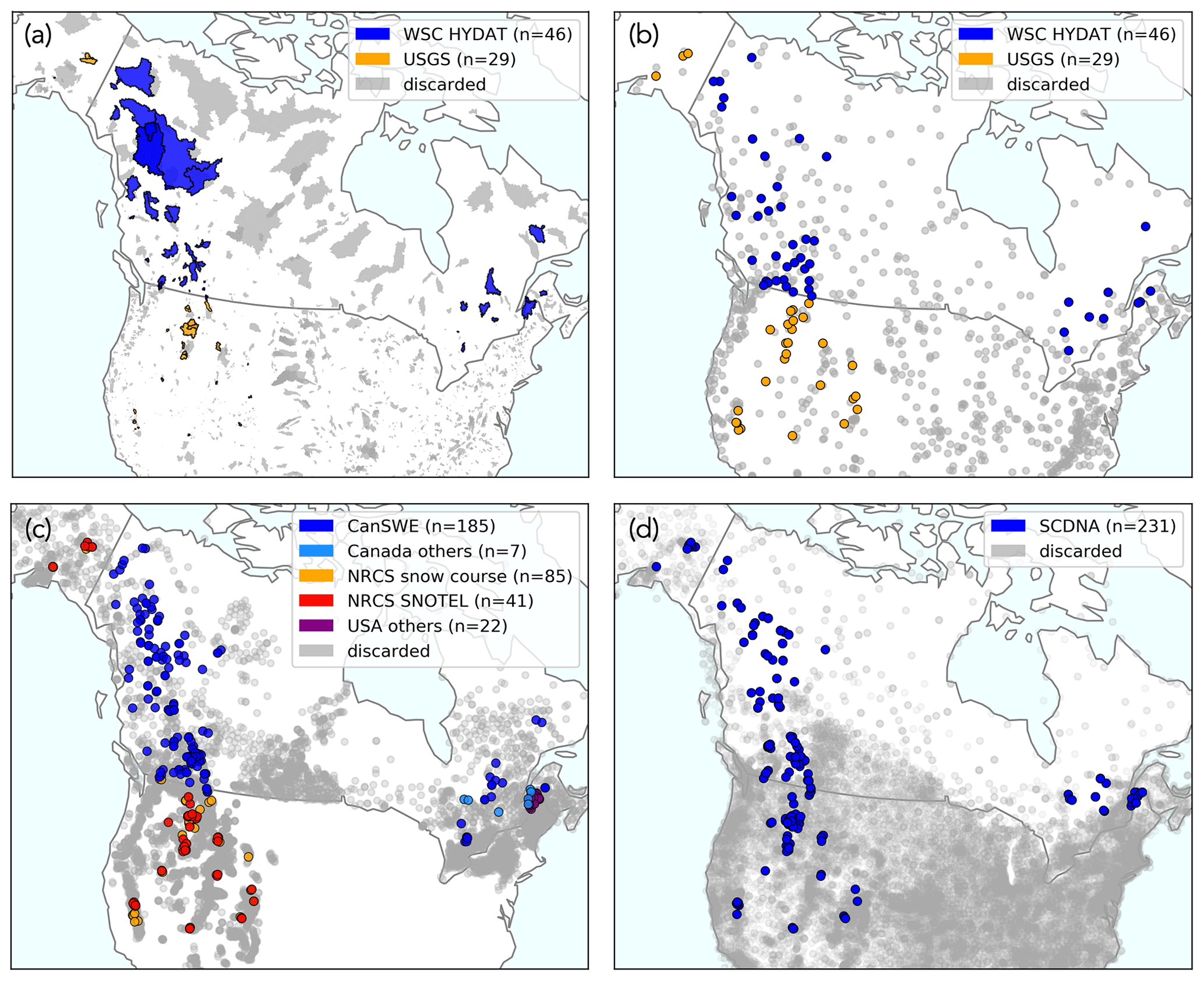
Figure 1 Maps of (a) basin outlines and input station data – i.e., (b) streamflow, (c) SWE, and (d) precipitation – across North America. Note that there are fewer streamflow stations than basin outlines, as map (b) only shows streamflow stations with data for the period 1979–2021. Basin outlines and input station data discarded and not used for the analysis presented in this paper are shown in grey (see the basin selection process in Sect. 2.2.1). Note that the maps are zoomed in on the retained elements, and some discarded basin outlines and stations may fall outside the map boundaries.

2.1.1 Basin shapefiles and streamflow data

For the USA, we use shapefiles and streamflow observations for basins with limited regulation from the USGS Hydro-Climatic Data Network 2009 (HCDN-2009; Lins, 2012; Falcone, 2011). HCDN-2009 comprises stations with minimal hydrological disturbance, measured by the presence of dams, freshwater withdrawal (including from groundwater, flow diversion, roads, and other impervious surface areas), and pollutant discharges. Moreover, inclusion in the dataset necessitates a minimum of 20 years of continuous availability of streamflow data.

For Canada, we use shapefiles and streamflow observations for basins with limited regulation from the Water Survey of Canada (WSC) HYDAT Reference Hydrometric Basin Network (RHBN) subset, called RHBN-N (ECCC, 2021). The selection criteria for the HCDN-2009 and RHBN datasets exhibit substantial similarity, albeit with potential methodological nuances that may stem from varying priorities and contexts. The reference hydrologic networks only include stations considered to have minimal or stable human impacts as defined by the presence of agricultural and urban areas, roads, a high population density, and the presence of significant flow structures (Whitfield et al., 2012). RHBN-N was created to provide a nationally balanced network suitable for national studies. Similarly to the HCDN-2009 dataset, a minimum data availability of 20 years of almost continuous streamflow records was required for a station to qualify.

We downloaded streamflow data for the period 1 January 1979 to 31 December 2021 as data for this period were available for many stations in the dataset, and this was deemed an appropriate time series length for the purpose of this study. Data for the USA were downloaded from the National Water Information System (NWIS; USGS, 2023) using the Python package dataretrieval (Hodson and Hariharan, 2023). Data for Canada were downloaded from the WSC HYDAT database (ECCC, 2018) using the EASYMORE Python package (Gharari et al., 2023). See Fig. 1a and b for maps of the basin shapefiles and streamflow stations that were retained.

2.1.2 Snow water equivalent data

SWE measurements were downloaded for the period 1 October 1979 to 31 July 2022. For Canada, measurements are from the Canadian historical Snow Water Equivalent dataset (CanSWE, Version V5; Vionnet et al., 2021b) available on Zenodo (Vionnet et al., 2023). CanSWE is a database of SWE data collected from numerous provincial, territorial, academic, and other agencies across Canada. Other measurements are from the Ministère de l'Environnement, de la Lutte contre les changements climatiques, de la Faune et des Parcs (MELCCFP) in Quebec (Canada) and cannot be shared publicly. For the western USA and Alaska, measurements are mainly from the Natural Resources Conservation Service (NRCS) manual snow surveys and Snow Telemetry (SNOTEL) automatic snow pillows. The NRCS snow courses can be downloaded using the following GitHub repository: https://github.com/CH-Earth/snowcourse (last access: 23 August 2024, Clark and Vionnet, 2021). For SNOTEL, we use data from the bias-corrected and quality-controlled (BCQC) dataset from the Pacific Northwest National Laboratory (PNNL; https://www.pnnl.gov/data-products, last access: 23 August 2024, PNNL, 2021; Sun et al., 2019; Yan et al., 2018). In the northeastern USA, manual snow survey data were obtained from local agencies in the states of Maine, New Hampshire, New York, and Vermont. All the snow survey data collected in the USA and used in this study are available in the SWE dataset of Mortimer and Vionnet (2024). Figure 1c shows a map of the SWE stations used for this analysis. Note that snow data are missing in the northern central part of the USA, and a viable substitute in the future could be to utilize airborne gamma snow data (Cho et al., 2020), as done by Mortimer et al. (2024) when validating gridded SWE products over North America.

All SWE data used for this study were quality-controlled. In addition to the quality standards applied by the different data providers, a systematic quality-control procedure is described in Vionnet et al. (2021b) and was applied to all the snow data used in this study, with the exception of the already bias-corrected and quality-controlled SNOTEL dataset.

Several SWE stations appear to be overlapping in Fig. 1c. In various Canadian provinces and territories like Alberta, British Columbia, and the Yukon, automated snow stations and manual snow surveys are collected at the same sites. While the measurements from these stations generally agree, they are not identical due to microscale spatial variability. In addition, the station overlap may partly be due to the scale of the map, which does not accurately display the variability of the snow measurement network in terms of position and elevation.

We use all available streamflow and SWE data and do not filter out data values based on their quality flags. The reason is that we perform gap-filling of all time series within the workflow, and we trust that data providers are the most competent individuals to handle the initial infilling. We invite readers to refer to these datasets for a list of quality flags.

2.1.3 Precipitation data

Precipitation station data were downloaded from the Serially Complete Dataset for North America (SCDNA, Version 1.1) for the period 1 January 1979 to 31 December 2018 (Tang et al., 2020a). The SCDNA dataset is available at Zenodo (Tang et al., 2020b). Figure 1d shows a map of the SCDNA stations.

2.2 Methods: workflow

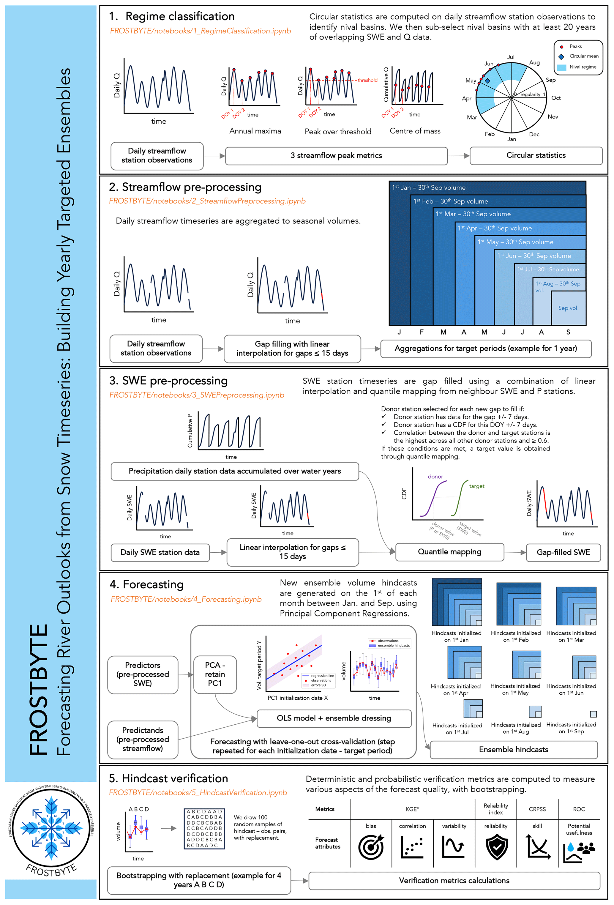
The workflow developed is structured into five Jupyter Notebooks: (1) regime classification, (2) streamflow preprocessing, (3) SWE preprocessing, (4) forecasting, and (5) hindcast verification. Each Notebook is coded in Python and provides concise descriptions of its purpose, decisions, and underlying assumptions, whenever necessary, as well as a step-by-step overview of the annotated code, accompanied by visuals. The workflow, called FROSTBYTE (Forecasting River Outlooks from Snow Timeseries: Building Yearly Targeted Ensembles), is available on GitHub (Arnal et al., 2024a, v1.0.0). Note that the data-downloading step (see Sect. 2.1) was not included in the GitHub workflow. Instead, sample data are provided for the Bow River at Banff (Alberta, Canada) and for the Crystal River above Avalanche Creek near Redstone (Colorado, USA). Figure 2 provides a visualization of the methods for each Jupyter Notebook. These will be described in more detail in the sections below.

Figure 2 Detailed graphical methods for each Jupyter Notebook of the FROSTBYTE workflow.

2.2.1 Regime classification: basin selection

To ensure the feasibility of producing forecasts using PCRs from SWE predictors, we impose the following requirements on the basins used in this study:

• The basin must have a nival regime. This is discussed in more detail in this section.

• The basin must contain at least one SWE station.

• The basin must have at least 20 years of overlapping SWE and streamflow data (partially incomplete years are allowed as the data are further processed to fill gaps; see Sects. 2.2.2 and 2.2.3). If the basin contains multiple SWE stations, only one station needs to fulfill this requirement.

The river basins in the USA and Canada for which we collected data in the previous step (see Sect. 2.1) are subject to a wide range of hydroclimatic conditions. In this step, we subset these basins to only keep those that experience nival regimes – i.e., basins for which we can reasonably expect SWE to have substantial predictability for streamflow forecasting. The existence of nival regimes can be inferred from climate classification schemes that account for the fraction of precipitation falling as snow in a given place. However, we instead opt to use an approach that identifies the typical flow regime for each basin based directly on the observed streamflow in that basin.

To classify the streamflow regimes, we used circular statistics (Burn et al., 2010). Circular statistics measure the timing and regularity of hydrological events such as flow peaks. For this study, three different streamflow peak metrics were used to provide more robust results than using a single metric, because strengths of one metric can compensate for weaknesses of another. Some of these weaknesses are discussed in Court (1962), Whitfield (2013), and Burn and Whitfield (2017).

The metrics used to identify peak flow events are (a) the streamflow annual maxima, (b) the streamflow peaks over threshold, and (c) the streamflow center of mass (i.e., the date on which 50 % of the water-year streamflow occurs; Court, 1962); see Fig. 2. For the peak-over-threshold metric (b), the threshold was defined as the smallest annual maximum streamflow observed during the historical period in each basin. All metrics were computed using a water year from 1 October to 30 September of the following calendar year to link winter snow accumulation to the current year's snowmelt. In order to maximize the number of available data, we first performed gap-filling through linear interpolation of the daily streamflow data. More information about the interpolation can be found in Sect. 2.2.2. Note that the streamflow interpolation was performed twice independently, once prior to the regime classification and once as part of the streamflow preprocessing, for a more logical workflow. The streamflow annual maxima (a) and center-of-mass (c) metrics required complete years of data (i.e., any water year with missing observations was discarded), while the peak-over-threshold (b) metric allowed for incomplete years of data to identify peak flow events.

For each metric, we then calculated the average date of occurrence for these peak flow events by determining the circular mean of all event dates (see Fig. 2). Additionally, we assessed the regularity of the peaks by calculating the spread in the dates of occurrence of these events. The regularity value, which ranges between 0 and 1, provides a measure of how consistent the event dates are. Larger values indicate a higher level of regularity in the dates. Equations used for the regime classification can be found in the Appendix. For each metric, we identified nival basins as those with an average date of occurrence of peak flow events between 1 March and 1 August and a regularity above or equal to 0.65 (defined based on results presented in Burn and Whitfield, 2023). We finally selected all nival basins identified by the three individual metrics.

The streamflow linear interpolation could have impacted the regime classification, leading to missed flow peaks, especially for smaller river basins with faster response times. Nevertheless, all the stations had nearly complete datasets, as this was a requirement for selection in the creation of both datasets (see Sect. 2.1.1). Furthermore, the use of three metrics for peak flow event identification, coupled with the utilization of the circular statistics method with a regularity threshold of 0.65, potentially mitigates some of these issues.

2.2.2 Streamflow preprocessing

We processed the daily streamflow data for all previously identified nival basins (see Sect. 2.2.1) and converted them to volumes that capture the spring freshet, which may be of interest to water users (e.g., for water supply management, hydropower generation, irrigation scheduling, or early warnings of floods and droughts). These volumes serve as the predictands for the forecasting process (see Sect. 2.2.4).

We first performed gap-filling through linear interpolation of the daily streamflow data in order to maximize the number of available data. The maximum allowable gap length for interpolation was set to 15 d, which is consistent with the SWE interpolation approach (see Sect. 2.2.3). Due to the data availability quality checks conducted during the production of the HCDN-2009 and RHBN streamflow datasets, a one-step gap-filling process was considered sufficient for streamflow, in contrast to the two-step gap-filling performed for SWE (see Sect. 2.2.3).

We then computed volumes for periods without any missing data for each nival basin: 1 January to 30 September, 1 February to 30 September, 1 March to 30 September, etc., until 1 to 30 September (see Fig. 2). Volumes are calculated by summing the daily streamflow observations over the time periods mentioned above. These volume aggregation periods will be referred to as “target periods” in the context of forecasting throughout this paper. The volume dataset was saved for all the basins as a NetCDF file.

2.2.3 SWE preprocessing

For each previously identified nival basin (see Sect. 2.2.1), we processed the SWE data to fill gaps because the subsequent principal component analysis (PCA) does not allow missing values. These preprocessed SWE data serve as the predictors for the forecasting process (see Sect. 2.2.4).

We selected SWE and precipitation (if any) stations located in each nival basin. The precipitation data are used to maximize the number of data available as predictors. They were accumulated over water years for each precipitation station to serve as proxies for SWE. To further enhance the availability of data, we applied linear interpolation to fill gaps in the daily SWE records. The maximum allowable gap length for interpolation was set to 15 d, which aligns with the streamflow interpolation approach described in Sect. 2.2.2 and with the window of ±7 d used in the subsequent steps.

After applying linear interpolation, we utilize quantile mapping to fill the remaining gaps using data from neighboring stations (see Fig. 2). Statistics necessary for the quantile mapping were calculated for all extracted SWE and precipitation stations. That is, a cumulative distribution function (CDF) was constructed for each station and for each day of the year (±7 d). A CDF could only be constructed when at least 10 data points were available. Spearman's rank correlation coefficients were calculated between each basin's SWE and precipitation station for each day of the year (±7 d). Correlations could only be calculated when a minimum of three data points were available. It is important to note that the minimum sample size criteria for the CDF and the correlation calculations are user-defined. For this study, they were set to the values mentioned above in order to balance the need for a sufficiently large sample size for reliable results with the goal of filling in as many gaps as possible. The impact of these decisions could be explored in future research.

We perform gap-filling using quantile mapping by looping over SWE stations. For each missing SWE data point at a target station (i.e., the station requiring gap-filling), a suitable SWE or precipitation donor station (i.e., the station providing data for infilling of the target station's gap) was identified based on the following criteria:

• The donor station must have data on or around the date to be filled (within a window of ±7 d).

• The target and donor stations should have a constructed CDF for the day of the year corresponding to the date to be filled.

• The correlation between the target station and the donor station should be highest amongst all potential donor stations and exceed a minimum correlation threshold of 0.6. Stations with correlations larger than but close to 0.5 could be deemed only marginally correlated. We require a strong positive correlation to ensure the quality of the gap-filling process and to set the threshold to 0.6 for a station to be accepted as a donor station.

Based on these criteria, the value from the donor station closest to the date requiring filling is used to estimate the target station's value on the missing value's date. Note that the automatic SWE stations have a higher temporal frequency than the manual snow surveys, which could make the automatic stations preferable as potential donor stations.

As a result, a new gap-filled SWE dataset was generated and saved for each nival basin as a NetCDF file. Estimated values were clearly distinguished from the original observations using a specific flag.

Additionally, we developed an artificial gap-filling function to enable users to assess the quality of the gap-filling process. Results are shown for the Bow River at Banff (Alberta, Canada), one of the workflow testbeds, in the Appendix (Figs. A1 and A2). We do not show results for all other river basins as the artificial gap-filling is not the primary focus of this study.

It is important to note that no threshold was set to define a total maximum allowable gap length for each station. Consequently, certain stations may have undergone substantial gap-filling, as can be seen in Fig. A2. However, we speculate that setting such a threshold would have been counterproductive, as it would have significantly decreased the number of SWE stations available as predictors, thereby affecting the quality of the hindcasts produced. Additionally, linear interpolation might have impacted the construction of CDFs for donor and target stations, possibly introducing inaccuracies into the gap-filled data. Nevertheless, we speculate that utilizing a station's own data for gap-filling via temporal interpolation could yield superior results compared to utilizing data from other stations, especially given the relatively gradual temporal variations in SWE.

2.2.4 Forecasting

Using the preprocessed predictors and predictands (see Sects. 2.2.2 and 2.2.3) as inputs to an ordinary least-squares (OLS) regression model, we generate time series of ensemble hindcasts for each nival basin. Hindcasts are initialized on the first day of each month between 1 January and 1 September (both ends included) for the target periods 1 January to 30 September, 1 February to 30 September, 1 March to 30 September, etc., until 1 to 30 September. See Fig. 2 for a graphical overview of the steps described below.

For each initialization date–target period combination, we first remove all years that have any missing values in the predictand and/or predictor datasets. We use a leave-one-out cross-validation approach for forecasting, whereby each data point in the dataset is sequentially withheld as a validation set, while the model is trained on the remaining data points. We require a minimum of 11 years of overlapping data in total, comprising 10 years for training the regression model and an additional year for generating the hindcast. Consequently, we may not be able to generate hindcasts for the specific nival basins previously identified in Sect. 2.2.1 and for specific initialization date–target period combinations.

We then transform the gap-filled SWE from Sect. 2.2.3 into principal components (PCs) to eliminate any intercorrelation between the SWE stations (Garen, 1992). PCA is a statistical method used to transform a set of intercorrelated variables into an equal number of uncorrelated variables. This step becomes particularly essential after gap-filling, which might have introduced additional correlation between the SWE stations. In addition, PCA is central to characterizing the spatiotemporal variability of a predictor variable. The first PC (i.e., the PC which captures most of the total variance in the set of variables) serves as the predictor for the forecasting process. In our analysis, on average the first PC explains 90 % of the total variance in the gap-filled SWE station dataset across all hindcast initialization dates and river basins. The explained variance of each principal component can be found in the Appendix (Fig. A3). We only select the first PC in order to avoid any overfitting that could be caused by having too many predictors and a short time series. In a subseasonal climate forecasting study, Baker et al. (2020) showed that even using only the first two PCs could lead to overfitting for many river basins of the contiguous USA. We acknowledge however that this is a topic that warrants further exploration and discuss this in more detail in Sect. 4.4. We conduct a PCA and fit a new model for each predictor–predictand combination.

We subsequently split the predictor–predictand data using a leave-one-out cross-validation approach. We fit an OLS regression model on all years available for training. We then apply this model to the predictor year that was excluded, resulting in a deterministic volume hindcast for the corresponding target period. An ensemble of 100 members is then generated from this deterministic hindcast by drawing random samples from a normal (Gaussian) distribution. The distribution has a mean of 0 and a standard deviation equal to the root mean squared error (RMSE) between the deterministic hindcasts and observations during the training period. We repeat this step until ensemble hindcasts have been generated for all years in the predictor–predictand dataset. It is important to note that hindcasts were generated only if there were at least 10 years of overlapping predictand–predictor training data for a given initialization date–target period combination.

An independent regression model is used to produce an ensemble hindcast for each river basin, initialization date, target period, and year left out. Once we have generated hindcast time series for all initialization date–target period combinations and all nival basins (when possible), each basin's hindcasts are individually saved in a new NetCDF file.

2.2.5 Hindcast verification

An overview of the various deterministic and probabilistic metrics used to assess the quality of the hindcasts, and what they measure, is provided in Table 1. To quantify the sampling uncertainty, all metrics are computed using bootstrapping (Clark et al., 2021b). We draw 100 random samples of hindcast–observation pairs, with replacement.

(Gupta et al., 2009)Tang et al. (2021)(Renard et al., 2010; Mendoza et al., 2017)(Hersbach, 2000)(Ferro et al., 2008; Ferro, 2014; Zamo and Naveau, 2018)(Mason and Graham, 2002)(Arnal et al., 2018; Emerton et al., 2018)

Table 1 Overview of the various deterministic and probabilistic metrics used to assess the quality of the hindcasts.

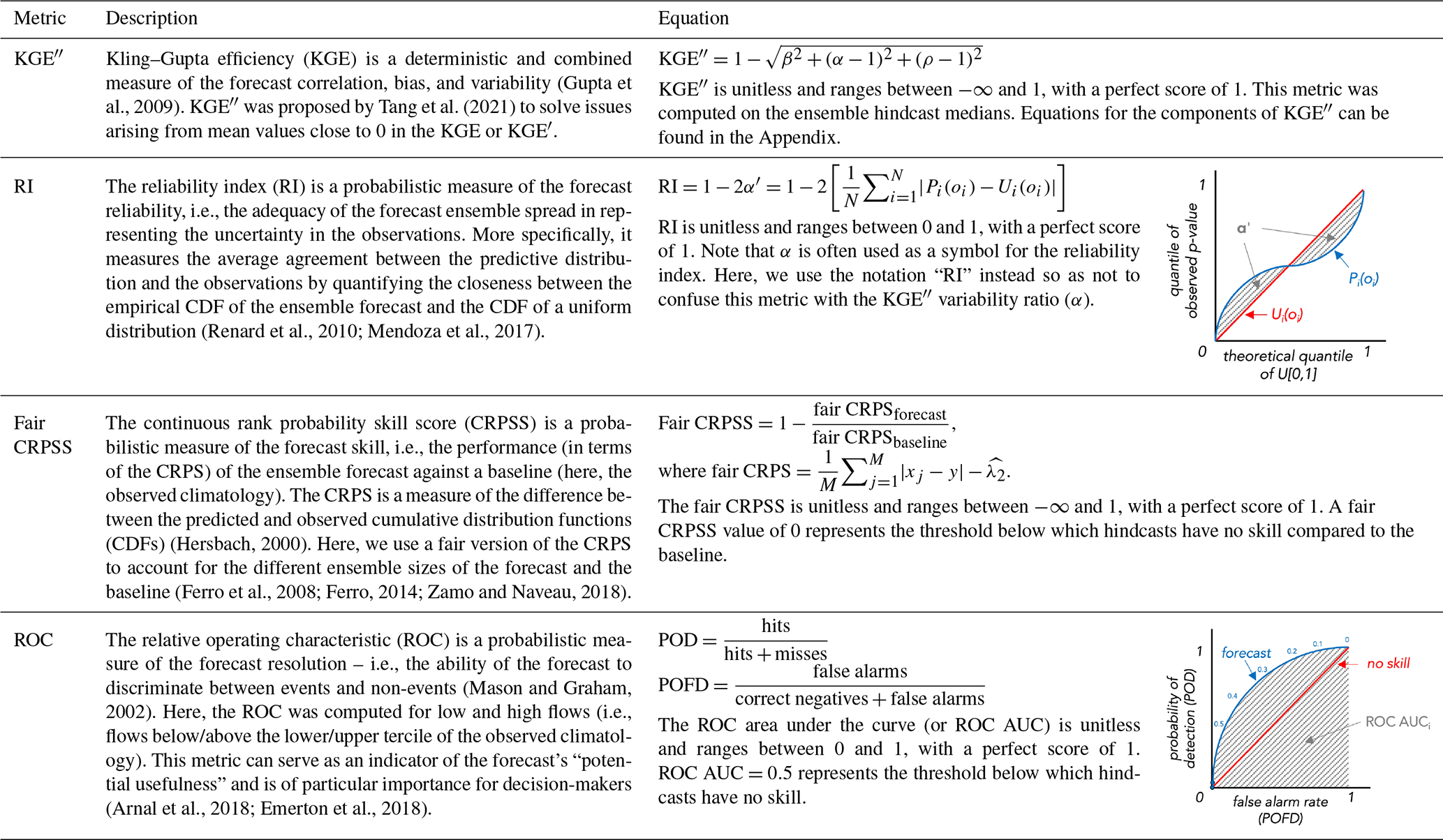
P_i(o_i): empirical CDF of the ensemble forecast p values for year i. U_i(o_i): uniform distribution U[0,1]. x_j: member j of the ensemble forecast with size M. y: corresponding observation. $\widehat{{\mathit{\lambda }}_{\mathrm{2}}}$: expectation of the CRPS, unbiased when the members are independently sampled from the forecast distribution (see Zamo and Naveau, 2018).

To enable a meaningful comparison of performance across different basins, we defined specific target periods that capture each basin's peak flow (Qmax). We refer to these periods as “periods of interest” throughout the paper. For each nival basin, the period of interest begins in the month of the basin's Qmax and extends until the end of the water year. For example, if a basin has its Qmax on 15 May, its period of interest will be 1 May to 30 September.

To guide the hindcast evaluation, we formulate two hypotheses regarding the hindcasts generated using these approaches:

1. The hindcast performance is expected to be better for hindcasts initialized around the peak SWE in each basin.

2. Higher hindcast quality is anticipated for hindcasts with high antecedent SWE content and low precipitation during the hindcast target period in each basin.

To support the interpretation of the hindcast evaluation and verify those hypotheses, we computed two additional measures. To evaluate the first hypothesis, we calculated the “SWE content” for all initialization dates (i.e., note that forecasts were initialized on the first day of each month between January and September for computational reasons and that we may as a result miss peak SWE). We calculated the median percentage of maximum SWE for each initialization date across all available years of data for all the SWE stations. The maximum SWE value was determined for each water year for this calculation. For example, a median percentage of maximum SWE of 50 % indicates that, across all years for which we have data for a given SWE station, in the median year half of that year's maximum SWE is present at that location on the forecast initialization date. The equation to calculate the SWE content can be found in the Appendix.

To evaluate the second hypothesis, we computed the ratio of precipitation to SWE (i.e., $P/\text{SWE}$). To achieve this, we followed these steps for each basin:

• We calculated the precipitation accumulation for each year, target period, and precipitation station within the basin. We then calculated the climatological medians for precipitation accumulation, considering each station and target period, and subsequently averaged them over the entire basin. This gave us the basin-averaged precipitation accumulation climatological medians for each target period.

• We calculated the SWE climatological median for each initialization date and each SWE station within the basin. We then averaged the SWE climatological medians over the entire basin, resulting in basin-averaged SWE climatological medians for each initialization date.

• Finally, we divided the basin-averaged precipitation statistics by the corresponding basin-averaged SWE statistics for each combination of initialization date and target period.

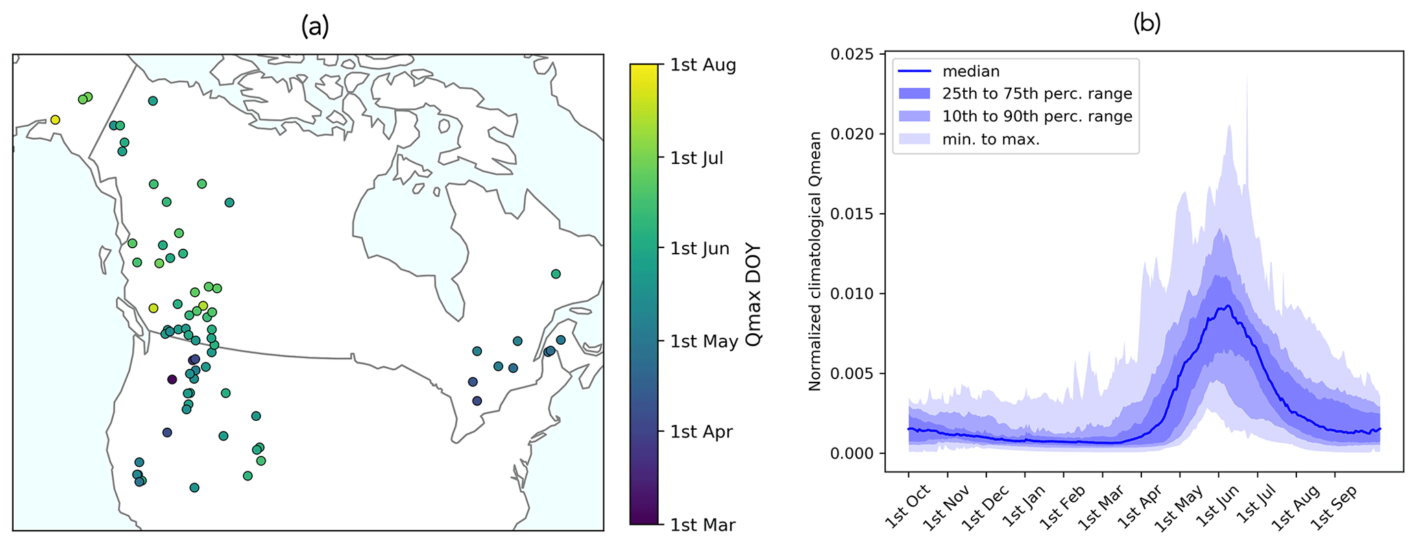
Figure 3 Map and hydrographs of the 75 nival basins with limited regulation that meet the data requirements. Basins identified as having a nival regime that did not meet the data requirements are shown in the Appendix (Fig. A4). (a) The map shows the average day of the year (DOY) when the maximum streamflow (Qmax) occurs for each nival basin. (b) The hydrographs display the normalized climatological mean streamflow for all 75 nival basins (i.e., the daily fraction of total annual streamflow), with the median across all basins as the blue line and the variation in responses across all basins indicated by the shaded percentiles.

3 Hindcast evaluation

In this section, we quantify the range of predictability for 62 of the 75 identified nival basins across North America (Fig. 3) by analyzing the results for various deterministic and probabilistic metrics, as outlined in Sect. 2.2.5. A total of 13 basins were excluded from this analysis as no hindcasts could be generated for those basins due to a limited number of overlapping predictor–predictand training data (as outlined in Sect. 2.2.4).

The figures presented in the subsections below display only the bootstrapping means. The corresponding bootstrapping ranges, showing the uncertainty in these estimates, can be found in the Appendix (Fig. A7).

3.1 Correlation, bias, and variability

Figure 4 shows the hindcast performance in terms of the Kling–Gupta efficiency (KGE^′′) and its decomposition into correlation, variability, and bias in the different subplots. In each subplot, results are shown for each hindcast target period (colored lines) as a function of hindcast initialization dates (x axis). Looking at the KGE^′′ for hindcasts produced for the target period 1 to 30 September (purple line) as an example, we observe the evolution in performance over time, from hindcasts initialized on 1 January (leftmost dot) to those initialized on 1 September (rightmost dot). The hindcasts' lead time decreases progressively from left to right within each subplot. The KGE^′′ can vary significantly across different target periods, and these differences tend to increase with later initialization dates. This highlights the impact of both target periods and the model initialization on the hindcast quality. Overall, the KGE^′′ is higher for the early target periods and decreases with the later target periods. This indicates that the snowpack holds less predictability as we move from the spring to summer and fall months and may be an indication of a shift from snow to rain as the dominant driver of streamflow.

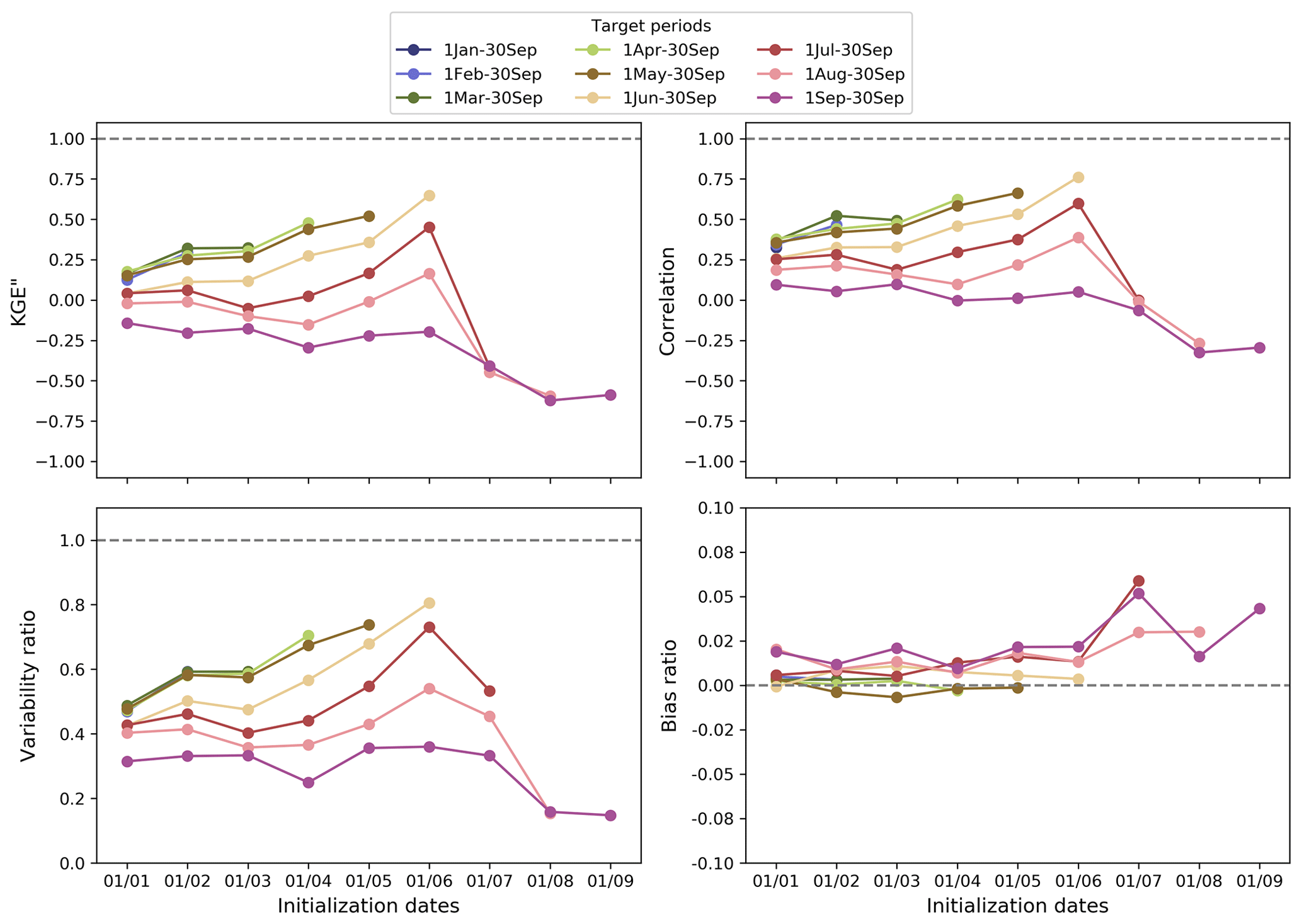
Figure 4 The KGE^′′ of the hindcast medians and its decomposition (i.e., correlation, variability, and bias) as a function of hindcast initialization dates. Each line displays the median values across all the basins for each target period. In all the plots, the dashed lines represent the perfect value for each metric. Refer to Table 1 for the KGE^′′ equation.

For hindcasts generated for the target periods 1 January to 30 September until 1 June to 30 September, the KGE^′′ increases towards the perfect value as we approach the start of the target period being predicted (i.e., with 0 lead months – e.g., hindcasts for 1 June to 30 September initialized on 1 June). Later target periods (1 August to 30 September and 1 to 30 September) show a declining KGE^′′ overall. Hindcasts for 1 July to 30 September show a mixed signal: they follow the later target periods' curves but with a peak for the 1 June initialization, after which they quickly decline.

The correlation and the variability ratio show similar patterns to the KGE^′′. The variability tends to be underestimated overall. This may be a direct consequence of using only PC1 as a predictor, although further comprehensive testing would be required to confirm this. The bias ratio is overall slightly positive, indicating that the hindcast medians overall overestimate the observed volumes. This is especially noticeable for hindcasts initialized between 1 July and 1 September.

Figure 5 Hindcast reliability as a function of hindcast initialization dates. The boxplots display values for all the basins. The dashed line represents the perfect value. Refer to Table 1 for the RI equation.

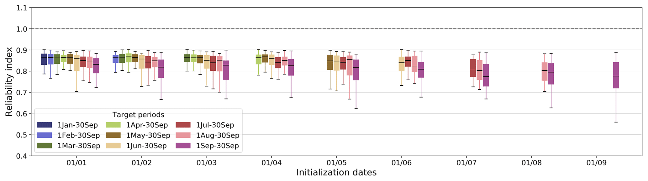
3.2 Reliability

Figure 5 shows the hindcast reliability, measured with the reliability index (RI), as a function of hindcast initialization dates. From the literature, we expect the hindcasts generated to have high reliability given the ensemble generation approach used (i.e., statistical analysis of errors in cross-validated hindcasts, compared to other methods, such as using an ensemble of models or an ensemble of meteorological inputs without any preprocessing). Indeed, overall, hindcasts display a high RI (ranging between 0.55 and 0.9) across all river basins, initialization dates, and target periods.

The reliability of hindcasts is not entirely perfect, which is primarily due to the leave-one-out cross-validation approach used. We expect this effect to be more noticeable when the sample size is smaller and hypothesize that it may partially account for the decrease in hindcast reliability with the increasing initialization dates observed here.

The lower reliability for the 1–30 September target period additionally provides further support for the diminishing significance of snow information during periods characterized by non-snowmelt-driven flow.

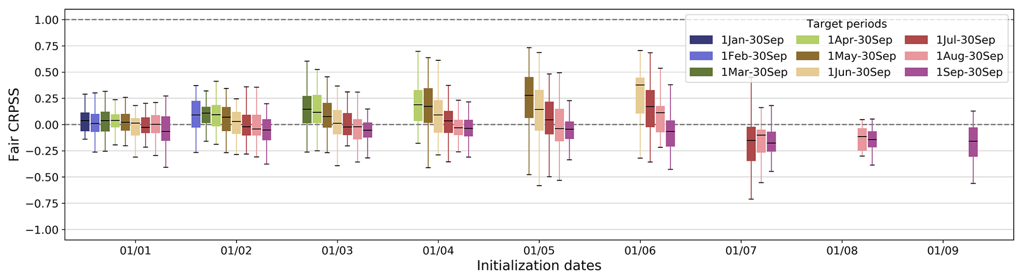
Figure 6 Hindcast fair CRPSS for each target period as a function of hindcast initialization dates. The boxplots display values for all of the basins. The upper dashed line (fair CRPSS=1) represents the perfect value, and the lower dashed line (fair CRPSS=0) represents the threshold below which hindcasts have no skill compared to the streamflow climatology. Refer to Table 1 for the fair CRPSS equation.

3.3 Skill

Figure 6 shows the hindcast skill in terms of the fair continuous rank probability skill score (fair CRPSS) as a function of hindcast initialization dates. On average, hindcasts are as good as the baseline when they are initialized on 1 January. They gradually get more skillful (i.e., better than the observed streamflow climatology) for initialization dates between 1 February and 1 June. Beyond 1 June, hindcasts for the summer–fall target periods exhibit no overall skill (i.e., worse than the observed streamflow climatology). Overall, earlier target periods have better skill than the later target periods. This is similar to the pattern observed for KGE^′′ and again hints at a shift from snow to rain as the dominant driver of streamflow. This further suggests that, as we approach the peak SWE (see Fig. 9a in Sect. 4.1), we can extract more valuable information and enhance the hindcast skill.

This SWE-based forecasting approach is unskillful with later initialization dates and target periods, meaning that using the streamflow climatology provides better results than using this approach. Note that the fair CRPSS results might be impacted by the ensemble size of the hindcasts (100 members) compared to the ensemble size of the baseline (the number of members equals the number of years in the climatology, excluding the year being forecasted, and varies across basins and target periods).

As shown by the boxplots' span, the fair CRPSS can vary considerably across basins. This implies that the predictive performance might differ significantly, depending on the geographical location. To explore the geographical distribution of the fair CRPSS, we show maps of the fair CRPSS with 0- to 6-month lead times (Fig. 7). Note that the lead months are different from the initialization dates of the hindcast, where lead month refers to the number of months between the hindcast initialization date and the target period start. The fair CRPSS maps show results for each basin's period of interest only, in order to be able to compare results across river basins for a single lead time. Overall, the fair CRPSS decreases with increasing lead time, and at a lead time of 3 or more months there is little skill evident. Note that some basins may show increasing skill with an increasing lead time or a more complex picture, highlighting the intricate interplay between initialization date and target period.

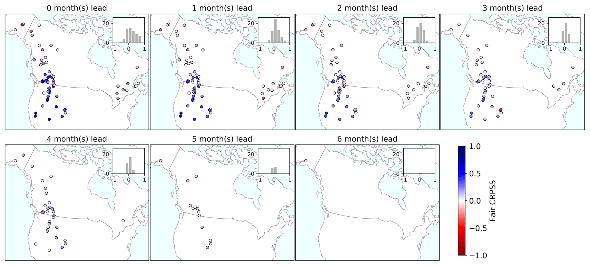
Figure 7 Maps of the hindcast fair CRPSS for hindcasts from 0- to 6-month lead times and inset histograms showing the distribution of fair CRPSS values. Each subplot shows results for the target period of interest in each river basin. Note that the initialization dates and periods of interest are not shown explicitly here. For instance, the first map, showing the fair CRPSS for hindcasts with a 0-month lead time, will include results from hindcasts of 1 January to 30 September initialized on 1 January as well as from hindcasts of 1 February to 30 September initialized on 1 February. On the other hand, the last map, showing the fair CRPSS for hindcasts with a 6-month lead time, will include results from hindcasts of 1 July to 30 September or later, initialized on 1 January or later. The number of river basins shown on each map varies based on the lead time, reflecting the period of interest being forecasted (e.g., a river basin with a 1 January to 30 September period of interest cannot be forecasted with more than a 0-month lead time after 1 January). The last subplot (i.e., a 6-month lead time) shows the results for a single river basin situated in Alaska.

The results are very variable across space and some river basins already show low to no or negative skill throughout the lead months, while the skill drops quickly after a 0-month lead time. These are mostly basins situated in the northwest and east. Pockets of higher skill are seen across several lead months for basins situated in western North America in and around the Rocky Mountains and Sierra Nevada ranges. Figure A5 displays river basins which consistently exhibit negative skill as well as those consistently demonstrating high skill. We speculate that basins exhibiting higher skill are those characterized by substantial contributions of SWE to streamflow predictability and by substantial year-to-year variability, thereby enhancing skill in comparison to the climatological reference.

3.4 Potential usefulness

Figure 8 shows the hindcast potential usefulness in terms of the relative operating characteristic area under the curve (ROC AUC) as a function of hindcast initialization dates for predicting (a) high flows and (b) low flows. Unlike the plots for KGE^′′ and its decomposition, the reliability index, and the fair CRPSS (boxplots only), these plots show the results for each basin's period of interest only, as we are interested in understanding the predictability of higher-than-normal or lower-than-normal volumes during the basin's peak-flow period. The results for low and high flows are very similar, which could be related to the high hindcast reliability and will be described jointly below.

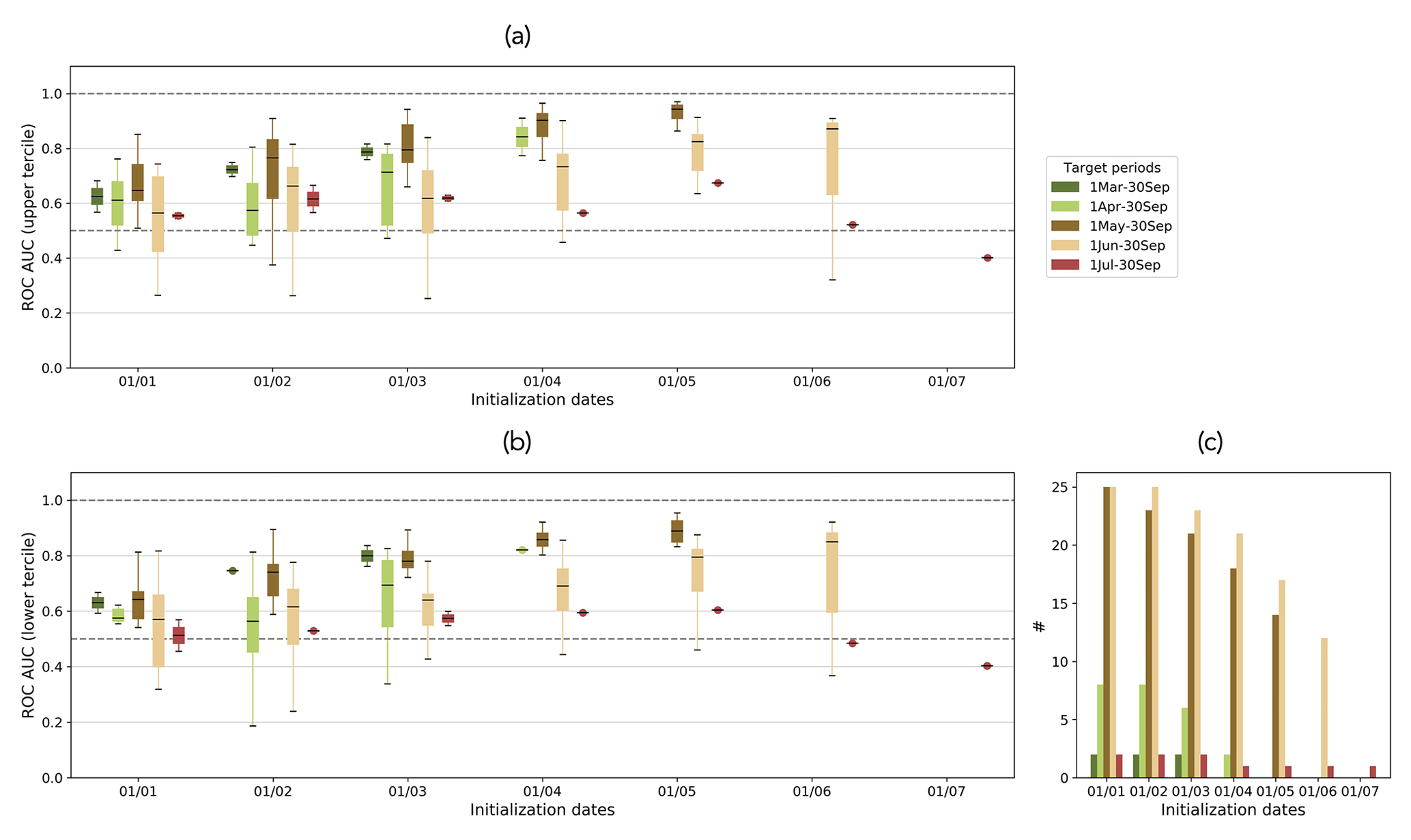
Figure 8 Hindcast ROC AUC for each target period as a function of hindcast initialization dates for (a) flows above the climatology's upper tercile and (b) flows below the climatology's lower tercile. The boxplots display values for all the basins, where their period of interest coincides with one of the target periods. The number of river basins in each boxplot is shown in panel (c). The upper dashed line (ROC AUC=1) represents the perfect value and the lower dashed line (ROC AUC=0.5) represents the threshold below which hindcasts have no skill. Refer to Table 1 for the ROC AUC calculation.

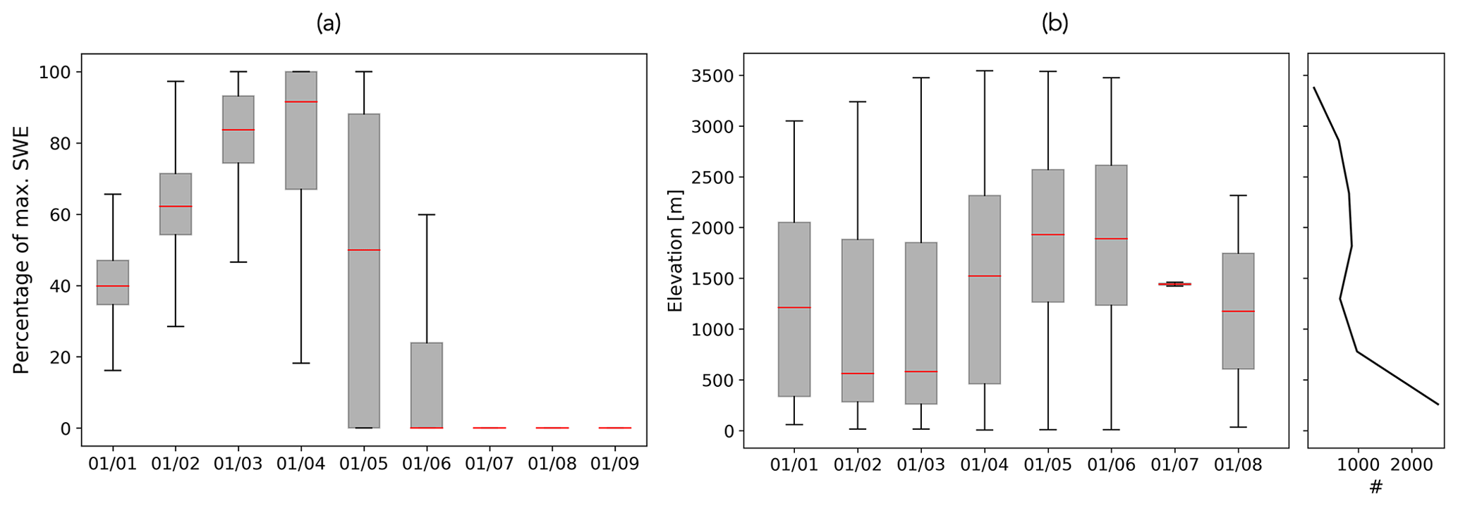
Figure 9 (a) SWE content on the first day of each month between 1 January and 1 September. (b) SWE station elevations as a function of the maximum SWE dates and the line histogram of the elevation of SWE stations.

For most of the target periods of interest, the peak ROC AUC is obtained for hindcasts with a 0-month lead time (a higher ROC AUC is better). For example, the ROC AUC of hindcasts for 1 May to 30 September is highest when the hindcasts are initialized on 1 May. The ROC AUC, and therefore the potential usefulness, of most hindcasts decreases with increasing lead times. This is however not the case for hindcasts for 1 July to 30 September, where the ROC AUC is highest when hindcasts are initialized on average on 1 May (with a 2-month lead time). This hints again at a shift from snow to rain as the dominant driver of streamflow between the spring and summer/fall months.

The hindcast potential usefulness varies for the different target periods, and the hindcasts generated for the target periods 1 March to 30 September and 1 May to 30 September show the best performances, indicating better predictions for low and high flows during these periods. Conversely, the hindcasts produced for the target periods 1 April to 30 September, 1 June to 30 September, and 1 July to 30 September exhibit the worst performances, implying less predictability for low and high flows for these specific periods. Overall, for all the periods of interest except for 1 July to 30 September there is potential usefulness in predicting low and high flows from 1 January.

As these plots show the results for each basin's period of interest only, some of the boxplots have a limited number of data points (i.e., the number of data points in each boxplot is shown in Fig. 8c). This could explain some of the differences between the boxplot span and the variability or noise observed in each subplot. Figure A6 in the Appendix shows the results for the individual basins.

4 User-oriented discussion

We now draw insights relevant for snow-monitoring experts, streamflow forecasters, decision-makers, and workflow developers from the results presented in Sect. 3.

4.1 Snow-monitoring experts

For this discussion, snow-monitoring experts include snow surveyors, field collection technicians, and monitoring network designers. Collectively, they conduct valuable work to support many different scientific and applied questions. An important use of snow surveys is water supply outlooks. As such, it is worth considering the following questions:

• Which SWE measurement dates are most important for forecasting streamflow volumes?

• Where and when are more SWE data needed for improving streamflow forecasts?

The first question relates to our first hypothesis that the highest performances can be found for hindcasts initialized around the peak SWE date in each basin (see Sect. 2.2.5). While peak SWE typically occurs around 1 April across North America (Fig. 9a), the results presented in Sect. 3 reveal that high performance in streamflow forecasts can still be achieved by using SWE observations up until 1 June. This suggests that persistent snowpack (i.e., after 1 April) can hold important predictability for spring and summer streamflow volumes. Thus, the SWE measurement dates after peak SWE are critical for skillful predictions of streamflow.

The importance of SWE measurement dates depends on the station elevation (and possibly also latitude; not shown). As seen in the boxplots in Fig. 9b, the timing of peak SWE exhibits a noticeable variation with station elevation, where, in general, stations situated at higher elevations have later peak SWE. On average, stations with peak SWE on 1 February and 1 March are at lower elevations than stations with peak SWE on 1 April, 1 May, and 1 June. It is evident in the accompanying line histogram in Fig. 9b that the majority of SWE stations are concentrated at lower elevations. While snow depth and SWE generally increase with elevation, the maximum snow depth in mountainous areas typically occurs near the tree line, with some variability across different sites due to variations in canopy cover (Cartwright et al., 2020; Grünewald et al., 2014). This suggests that SWE measurements at middle to high elevations best capture the peak SWE in these basins.

This brings us to the second question: where and when are more SWE data needed to improve streamflow forecasts? Given the importance of mid- to high-elevation SWE and the limited measurements at these elevations, measurement dates later in the snow season are necessary to capture the timing and magnitude of the maximum SWE and the evolution of snowmelt to predict snowmelt-driven runoff. Investigating the use of snow pillows, snow scales, and snow depth sensors is recommended to provide continuous depth and SWE measurements at point-based survey sites, thus increasing SWE temporal coverage. Expanding the spatial coverage of point-based surveys to include more mid- to high-elevation areas may pose challenges due to the difficulty in reaching these locations and the manual labor needed to set up and maintain such sites. This work can hopefully serve as a guide to getting the maximum amount of useful data out of limited observation networks and budgets. Exploring ways to augment SWE spatial coverage may additionally involve replacing point-based SWE data with alternative sources such as remote sensing techniques like lidar (Painter et al., 2016) or leveraging gridded snow products like SnowCast (http://www.snowcast.ca, last access: 23 August 2024; Vionnet et al., 2021a) (Mortimer et al., 2020).

This discussion leads further to questions about how additional SWE measurements can improve the quality of streamflow forecasts. There are instances where manual SWE measurements fail to accurately capture the peak snowpack (which is particularly problematic in the absence of automatic snow measurements within the basin). On top of this, the forecasting strategy utilized here (i.e., initializing forecasts on the first day of each month) may also miss the peak snowpack. To address this, exploring more frequent predictions, like initializing and updating forecasts in the middle of each month, could prove beneficial. Additional research aimed at enhancing snow-surveying networks could concentrate on identifying station locations that are representative of the basin SWE on different dates. These specific sites could then be targeted for additional point measurements or continuous monitoring using snow pillows, snow scales, or snow depth sensors to ensure comprehensive capturing of mid-month peak SWE events.

4.2 Forecasters

According to our second hypothesis, we expect higher hindcast quality for hindcasts with high antecedent SWE content and low precipitation during the hindcast target period in each basin (see Sect. 2.2.5). We quantify the impact of antecedent snowpack vs. future precipitation on the hindcast performance. Figure 10 shows the $P/\text{SWE}$ ratio (see Sect. 2.2.5 for more information on its calculation) as a function of the hindcast fair CRPSS for each target period. As anticipated, for most target periods, the hindcast skill increases as the $P/\text{SWE}$ ratio decreases. This suggests that the hindcasts are more skillful when the initialization date snowpack increases and/or when the target period precipitation proportion decreases. However, this relationship varies across different target periods. There is a stronger correlation (with statistical significance) for hindcasts generated for the target periods 1 March to 30 September, 1 April to 30 September, and 1 May to 30 September (Fig. 10c, d and e, respectively). Furthermore, this relationship does not hold for the target periods 1 August to 30 September and 1 to 30 September (Fig. 10h and i, respectively).

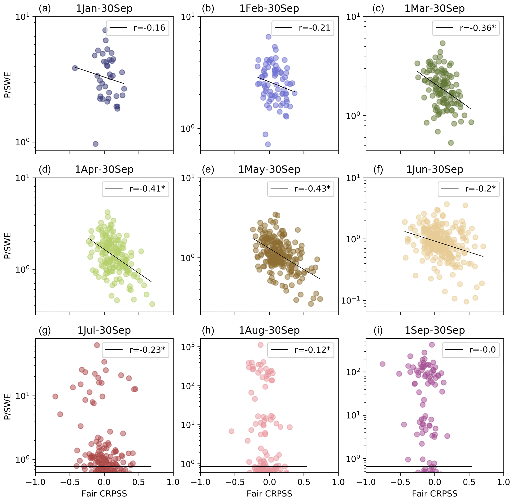
Figure 10 $P/\text{SWE}$ as a function of the hindcast fair CRPSS for all the hindcast initialization dates and all the basins for each target period (subplots). Each point represents the result for a given basin and initialization date. The Pearson correlation coefficient (r) is shown in the top right of each plot, where the asterisk denotes the statistical significance at a 5 % significance level.

This figure emphasizes the sensitivity of the results to the flow regime, raising concerns about potential loss of predictability with a changing (snow) climate. According to the Sixth Assessment Report of the Intergovernmental Panel on Climate Change (IPCC, 2021, 2022), snow extent, snow cover duration, and accumulated snowpack are virtually certain to decline in subarctic regions of North America. There is also a projected decrease in seasonal snow cover extent and mass at middle to high latitudes and at high elevations. Hale et al. (2023) reported that the annual snow storage decreased in over 25 % of mountainous areas in western North America between 1950 and 2013 as a result of earlier snowmelt and rainfall in the spring months and declined in winter precipitation.

These changes are predicted to result in snow-related hydrological changes, including declines in snowmelt runoff (except in glacier-fed river basins, where the opposite might be true on shorter timescales) (IPCC, 2021, 2022), more frequent rain-on-snow events at higher elevations (where seasonal snow cover persists) due to a shift from snowfall to rain (Musselman et al., 2018), and consecutive snow drought years in western North America. Berghuijs et al. (2014) showed that a change in the precipitation phase from snow to rain significantly decreases the mean streamflow within individual catchments of the contiguous USA. In snow-dominated regions globally, there is high confidence that peak flows associated with spring snowmelt will occur earlier in the year. This effect has already been documented by several studies that show that new record peak flows fall into time periods outside the nival window (Gillett et al., 2022). Burn and Whitfield (2023) additionally discuss an increasing frequency of rainfall-driven peaks and floods.

As a result of these changes, we expect that the relationships between the SWE and streamflow will be affected, impacting the quality of snow-based streamflow forecasts in the future. Pagano et al. (2004) found that increasing hydrological variability in the western USA was partly responsible for the decline in the water supply forecast skill.

The analysis presented here showcases a wide spectrum of predictability, where basins encompass diverse geographies and climates ranging from purely nival regimes to mixed regimes. This spectrum of predictability can be appreciated in more depth in Fig. A7. This offers a glimpse into the potential changes in predictability we may observe in the future. To tackle these questions more thoroughly, future research could look at the impact of snow climate on these results. Additionally, investigating different cross-validation approaches could be influential in maintaining forecast quality over time.

In the study by Zheng et al. (2018), inner mountain areas in the western USA (dominated by snowmelt contribution) showed longer streamflow predictability, while coastal areas (dominated by rainfall contribution) had shorter streamflow predictability. While we selected river basins with a nival regime, we do also notice the influence of future unknown rainfall on these results (see Fig. 10). Figure 7 illustrates higher and longer predictability in interior and western North American river basins, contrasting with lower and shorter predictability in the north and in the east, which partly aligns with the findings of Zheng et al. (2018). However, further analysis is needed to identify spatial patterns in the hindcast skill and their relationships with the physical processes of runoff generation.

Climate predictors can add to the seasonal streamflow forecast skill available from the SWE, especially for basins with strong teleconnections between large-scale climate and local meteorology on longer timescales (Wood et al., 2016; Mendoza et al., 2017). Furthermore, Slater and Villarini (2017) found precipitation variability to be crucial for modeling high flows, while antecedent wetness impacts low and median flows in the US Midwest. They also found that temperature enhances model fits during snowmelt or high-evapotranspiration seasons. Lehner et al. (2017) found that the addition of temperature forecast information to operational seasonal streamflow predictions in snowmelt-driven basins within the southwestern USA not only enhances the skill of streamflow forecasts but also contributes to mitigating errors in streamflow predictions caused by climate nonstationarity. Antecedent streamflow can also be a strong predictor of future streamflow, as shown by Veiga et al. (2014).

These variables might enhance predictability and warrant exploration. However, the predictability sources vary depending on the initialization date, predictand, basin location, and hydroclimatic features (Wood et al., 2016). Even within a small domain, the relative importance of predictors can differ (Mendoza et al., 2017), emphasizing the need for detailed analysis to put forward additional basin-specific predictors. Tools like PyForecast (https://github.com/usbr/PyForecast, last access: 23 August 2024) could aid in exploring additional predictors for accurate ensemble seasonal volume forecasts within specific river basins or regions using the workflow presented here.

Additionally, embracing more flexible yet physically accurate forecasting methods is a logical progression. Hybrid methods that combine the strengths of machine learning with process-based models grounded in our comprehension of physical processes emerge as a reasonable choice for enhancing predictability over longer timescales (Slater et al., 2023). In recent studies, Chang et al. (2023) demonstrated the extended predictability of subseasonal hydrological forecasts in Switzerland by incorporating large-scale atmospheric circulation information. Additionally, Hauswirth et al. (2023) introduced a flexible and efficient hybrid framework that utilized global seasonal forecasts as inputs to produce skillful location-specific seasonal forecast information.

4.3 Decision-makers

This study focused solely on forecasting streamflows in unregulated river basins, which may include river basins upstream of a regulation, such as a reservoir or an urbanized area. Regulation alters the relationship between the hydrometeorological drivers of streamflow and streamflow. In those regulated river basins, it is however still valuable to predict streamflows upstream of the regulation (e.g., the inflows to a reservoir, streamflows upstream of a city or of a regulated river segment), where predictability comes from upstream SWE stations for water management decision-making downstream (e.g., for water supply management, hydropower generation, irrigation scheduling, early warnings of floods and droughts, riverine transportation). This methodology could additionally add value in regulated catchments where the naturalized flow is used for water management decision-making.

Forecast reliability plays a crucial role in facilitating risk-based decision-making (Zhao et al., 2016; Mendoza et al., 2017), e.g., in determining optimal water release volumes and schedules for hydropower generation and irrigation or in issuing timely warnings of potential high or low flows. High forecast reliability in turn instills trust in forecasts for informed decision-making (note that reliability is only one of many factors that contribute to user trust). Insights from the analysis of a serious game conducted by Crochemore et al. (2021) underscore the importance of high reliability for decision-making. Notably, the study revealed that decision-makers considered high reliability to be crucial, especially for risk-based decision-making in extreme years.

One of the distinguishing strengths of statistical forecasts, such as the ones generated here, over process-based forecasts lies in their ability to achieve high forecast reliability, stemming from the ensemble generation method employed. This aligns with the findings of Mendoza et al. (2017), who found that the regression-based forecasting methods they examined exhibited higher reliability than the process-based forecasting methods. For five case study sites across the US Pacific Northwest, their regression-based methods achieved reliability index values ranging between 0.6 and nearly 1, while the reliability of the process-based ensemble streamflow prediction (ESP) hindcasts declined when approaching the 1 April initialization date, with an overall reliability index ranging between 0.4 and 0.9. Our approach yielded reliability index values comparable to those obtained from the statistical methods developed by Mendoza et al. (2017). Emerton et al. (2018) found that the process-based seasonal streamflow forecasts produced within the Global Flood Awareness System (GloFAS) had limited reliability globally, with some spatial variability.

A fundamental question that arises pertains to the temporal horizon within which decisions can be confidently made. To provide some initial insights for decision-making, we provide matrices showing the evolution of the forecasts' potential usefulness for predicting low and high flows within specific river basins with increasing lead times, considering the period of interest within each basin (Fig. A6). However, the answer to this question is inherently user-specific and depends on factors such as the choice of the baseline, target periods, and specific events or thresholds of interest. To address these specific user requirements, further analysis is essential. This can be achieved by building on the provided codes and tailoring the forecasting methodology to align with distinct user needs.

In the context of operational forecasting, forecast consistency is a critical aspect for ensuring coherent decisions throughout the decision-making period. Considering the findings presented in this paper from an operational forecasting standpoint, a few methodological decisions may have affected the results. In this analysis, we conducted a PCA and established new models for each predictor–predictand combination and each year left out. We adopted a leave-one-out cross-validation approach due to limited data in certain basins, leveraging all available data to generate new hindcasts. It is important to acknowledge that this approach might introduce inconsistency from month to month and from year to year (Garen, 1992), together with some artificial quality in the hindcast verification process (DelSole and Shukla, 2009). In operational scenarios, forecasters may opt to use pre-existing PC matrices and models to ensure forecast consistency and smooth decision-making. However, this could be problematic in the case of nonstationary input data (Shen et al., 2022). This topic warrants further attention.

4.4 Workflow developers

Reproducibility of research in the water sciences is still very low (Stagge et al., 2019). This contributes to the typically slow transfer of research to operations. While journal policies are moving towards more open science (e.g., Blöschl et al., 2014; Clark et al., 2021a), such policies are not yet at the stage where full workflows must be published alongside a paper – though this seems a logical next step.

Building workflows that are both intuitive (i.e., that can represent our understanding of local hydrometeorological processes; Veiga et al., 2014) and reproducible is essential for providing platforms for progressive and purposeful testing of new scientific advances and for paving the way for applying research outcomes in practice. Furthermore, this fosters more equitable water research and education (Castronova et al., 2023).

However, it is important to acknowledge that the demands of scientific journals for open-source data and methods may sometimes conflict with the rapid and competitive nature of some environments, including academia. Striking a balance between open collaboration and maintaining a competitive edge poses challenges that the academic community must address. Explicitly acknowledging a researcher's commitment to the transparency, reproducibility, and reusability of their work during merit reviews is one possible step forward.

The workflow developed as part of this study adheres to the principles of open and collaborative science, facilitated by its design (i.e., Jupyter Notebooks) and code-sharing (i.e., GitHub). In line with the recommendations by Knoben et al. (2022), our approach prioritizes clarity, modularity, and traceability in the workflow design. This enables users to easily adapt the workflow for any river basin in the USGS or WSC HYDAT datasets. Users have the flexibility to modify, enhance, or replace specific components of the workflow to suit their needs. Below is a non-exhaustive list of future research ideas.

• In Notebook 1, one could look into replacing the regime classification component of this workflow with an alternative method to identify basins with a nival regime (such as using the fraction of precipitation falling as snow).

• In Notebook 2, we set the end of the water year as the endpoint for all forecast target periods in all river basins. However, some of these river basins may experience late summer to early fall rainfall events. For example, river basins in the east can be impacted by extratropical storms during that time of year and show a mixed hydrological regime (Burn et al., 2016). While we discarded most of these river basins through the strict regime classification and basin selection, it could be that some of these river basins were retained, affecting the forecast quality.

• In Notebook 3, we note the following:

  • Future research could explore the impact of using different gap-filling methods. Examples are the various gap-filling strategies explored by Tang et al. (2020a) for meteorological-station infilling to create the SCDNA dataset.

  • We used the SCDNA precipitation data for infilling, which do not distinguish between solid and liquid precipitation. Additionally, the precipitation was accumulated during the entire water year and did not consider the onset of snowmelt. Both of these decisions could have led to lower correlations between the SWE and the cumulative precipitation to identify suitable donor stations.

  • The selection of SWE stations used as predictors could play a significant role in the forecast quality. To improve SWE sampling, future research may consider expanding the station selection to include those within a buffer of the basin. Although this method was coded as part of the workflow, it was not implemented in this paper due to the need for a more comprehensive analysis of its impact on forecast quality.

  • Subsequent studies could investigate how various methodological choices influence the quality and effectiveness of the gap-filling, using the artificial gap-filling function. This could involve examining the consequences of implementing a total maximum allowable gap length to sub-select stations or adjusting the window used for the gap-filling through quantile mapping.

• In Notebook 4, we note the following:

  • There was no established minimum threshold for the percentage of variance that PC1 should explain in order to be used as a predictor. In addition, although the ability to use additional PCs was also coded as part of the workflow, it was not explored further in this paper in order to avoid overfitting. There are various methodologies around stopping criteria for including predictors, such as the Bayesian information criterion (BIC) or regularization approaches that can lessen the risk of overfitting (Baker et al., 2020). Investigating the effects of using additional PCs could lead to valuable insights. For instance, this could provide a means of investigating whether this accounts for the consistently underestimated variability.

  • Subsequent studies may explore a range of cross-validation strategies (e.g., sample-splitting, increasing the number of omitted years or excluding extreme years from the training dataset) to assess how they affect the quality of the generated hindcasts.

5 Conclusions

We developed a systematic and reproducible data-driven workflow for probabilistic seasonal streamflow forecasting in snow-fed river basins across North America, including Canada and the USA. This structured workflow consists of five essential steps: (1) regime classification and basin selection, (2) streamflow preprocessing, (3) SWE preprocessing, (4) forecasting, and (5) hindcast verification. This methodology was applied to 75 basins characterized by a nival (snowmelt-driven) regime and limited regulation across diverse North American geographies and climates. The input data, spanning from 1979 to 2021, include SWE (predictor), precipitation (for gap-filling), and streamflow (predictand) station data. The ensemble hindcasts were generated monthly, with initialization dates ranging from 1 January to 1 September and target periods from 1 January to 30 September, from 1 February to 30 September, etc. We analyzed the hindcasts using deterministic metrics (i.e., KGE^′′ and its decomposition to measure correlation, bias, and variability) and probabilistic metrics (i.e., the reliability index, fair CRPSS, and ROC AUC to measure reliability, skill, and potential usefulness, respectively). The insights derived from this comprehensive analysis are invaluable for snow-monitoring experts, forecasters, decision-makers, and workflow developers.

The key findings include the following.

• For snow-monitoring experts: the late-season snowpack (i.e., after 1 April) has significant predictability for spring and summer volumes. Thus, capturing the snowpack beyond the peak period is crucial for skillful predictions.

• For forecasters: higher hindcast skill is achievable using this forecasting approach for target periods when basins exhibit high antecedent SWE content and low precipitation during the forecast period. In many river basins and at many times of the year, the SWE is not a key predictor. Therefore, an optimal approach should leverage climate predictors to achieve a more comprehensive balance between the initial conditions and meteorological forcings that contribute to the predictability of runoff.

• For decision-makers: this statistical forecasting approach, not unlike other statistical forecasting approaches, can generate ensemble hindcasts that are statistically reliable. Moreover, for all periods of interest up to and including 1 June to 30 September, we can predict lower-than-normal and higher-than-normal streamflows with lead times of up to 5 months.

• For workflow developers: the developed workflow, shared as Jupyter Notebooks on GitHub, follows the principles of open and collaborative science. Its design is clear, modular, traceable, intuitive, and reproducible. This in turn facilitates applications in other cold regions and the advancement of methods based on the benchmark provided. We invite others to build upon this workflow and have outlined potential improvements in Sect. 4.4.

This study contributes to the existing research by (1) expanding the spatial scope to encompass both Canada and the USA, (2) creating a completely open and reproducible workflow, and (3) offering practical guidance for diverse users.

Appendix A: Additional figures

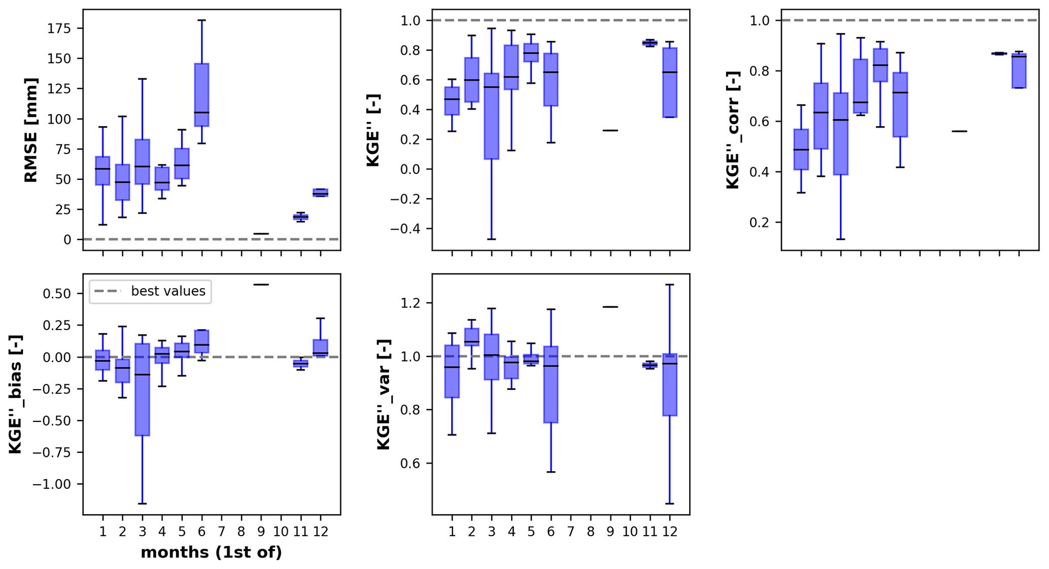
Figure A1 Performance metrics obtained from the artificial gap-filling step for the Bow River at Banff (Alberta, Canada). The boxplots contain results for all the SWE stations within the river basin.

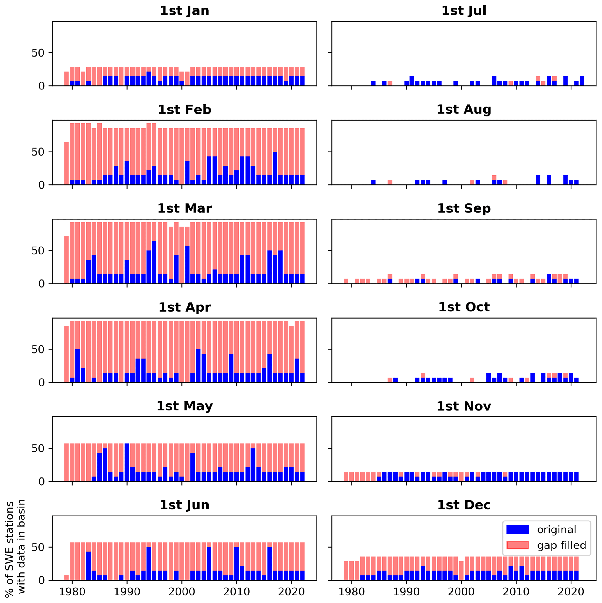
Figure A2 Time series of the availability of SWE station data on the first day of each month (subplots) before and after gap-filling for the Bow River at Banff (Alberta, Canada).

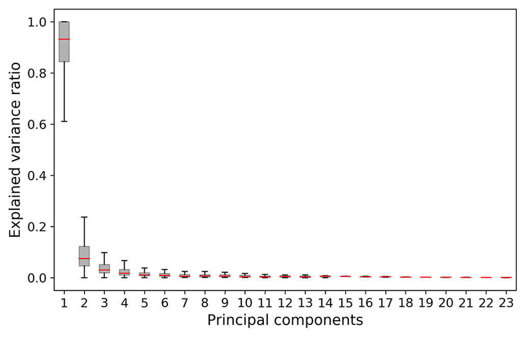
Figure A3 Explained variance for all the SWE principal components. The boxplots display values for all the hindcast initialization dates and basins.

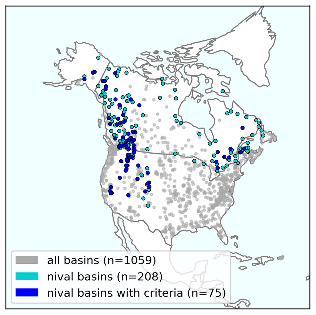
Figure A4 Map of all North American basins with data for the period 1979–2021 and with limited regulation (grey), identified nival basins (turquoise), and the subset of nival basins meeting the data requirements for the forecasting analysis presented in this paper (dark blue).

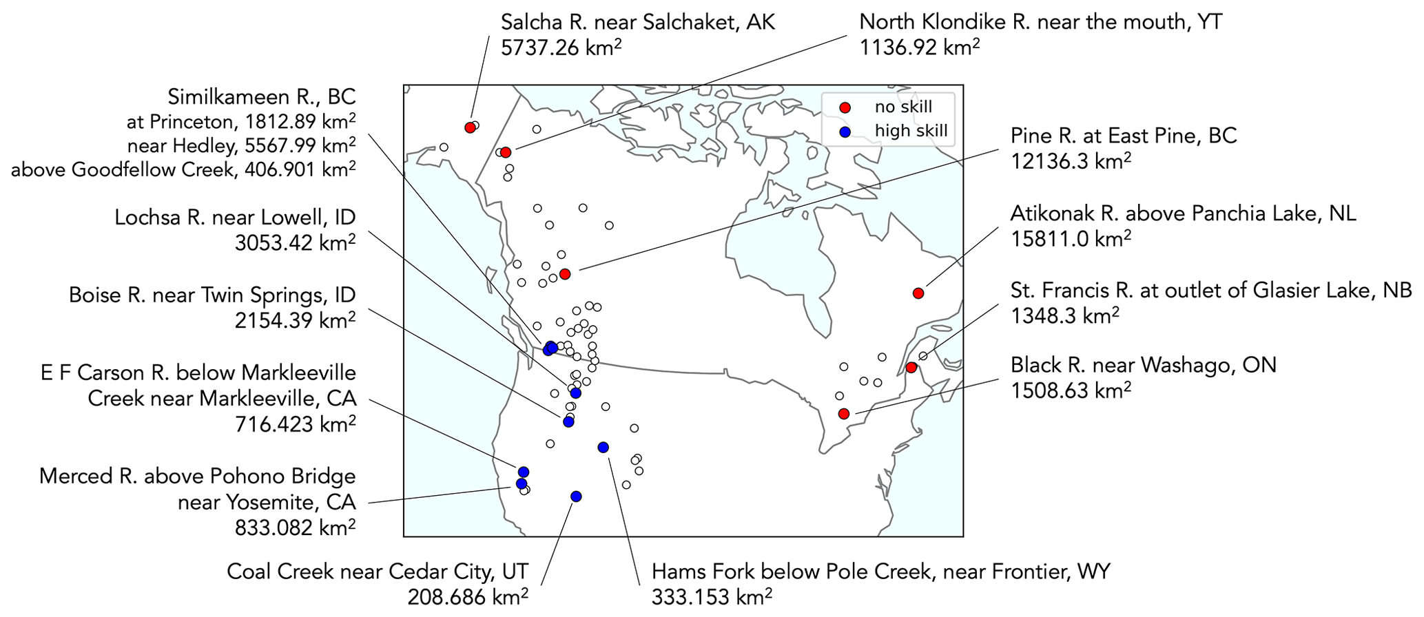
Figure A5 Map highlighting river basins in which skill consistently falls below zero (fair CRPSS<0 across all lead months for the basin's target period of interest; red) and those exhibiting consistently high skill (fair CRPSS≥0.5 across all lead months for the basin's target period of interest; blue).

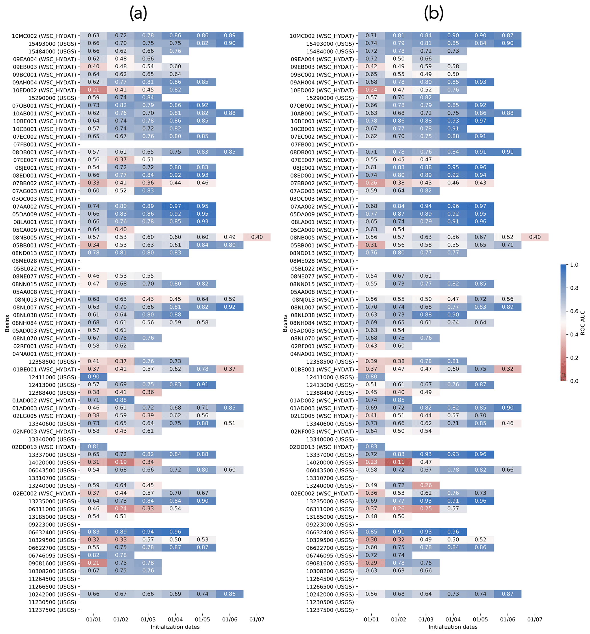
Figure A6 Hindcast ROC AUC for each basin as a function of initialization dates (a) for flows below the lower tercile of the climatology and (b) for flows above the upper tercile of the climatology (right). Results are shown only for each basin's period of interest. Basins are ordered from north to south, based on their latitudes. Blue colors show potentially useful hindcasts, and red colors show hindcasts with no skill.

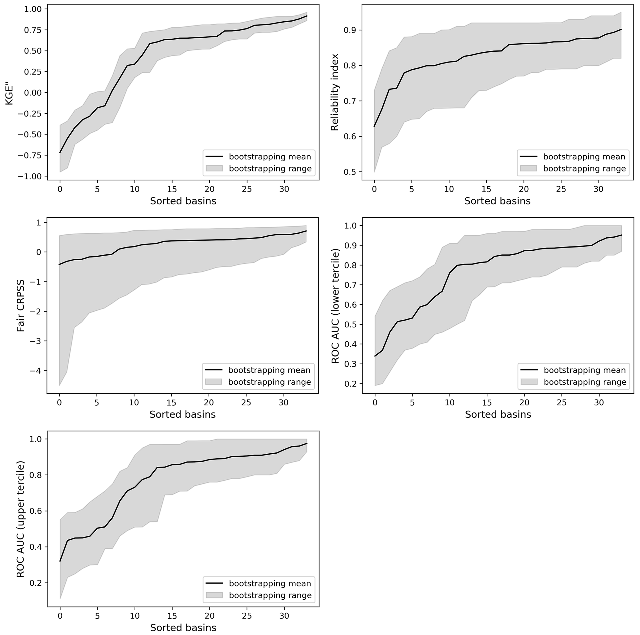
Figure A7 Bootstrapping mean and range (5th to 95th percentiles) for various metrics across the selected nival river basins (sorted from the lowest to highest mean metric values). Results are shown for 1 June to 30 September hindcasts generated on 1 June for illustrative purposes.

Appendix B: Circular statistics

The equations used for the regime classification were taken from Burn et al. (2010). The date of occurrence of an event (i) is defined by converting the Julian date to an angular value (θ_i; in radians) using the formula

$$\begin{array}{}\text{(B1)}& {\mathit{\theta }}_i=\left({\text{Julian date}}_i\right)\left({\displaystyle \frac{\mathrm{2}\mathit{\pi }}{\text{lenyr}}}\right),\end{array}$$

where lenyr is the number of days in a year.

From a sample of n events, we can find the x and y coordinates of the mean date with the following formulas:

$$\begin{array}{}\text{(B2)}& {\displaystyle }& {\displaystyle }\stackrel{\mathrm{‾}}{x}={\displaystyle \frac{\mathrm{1}}{n}}\sum _{i=\mathrm{1}}^n\cos {\mathit{\theta }}_i,\text{(B3)}& {\displaystyle }& {\displaystyle }\stackrel{\mathrm{‾}}{y}={\displaystyle \frac{\mathrm{1}}{n}}\sum _{i=\mathrm{1}}^n\sin {\mathit{\theta }}_i.\end{array}$$

The mean date (MD), or the average date of occurrence of all events i, can then be obtained with

$$\begin{array}{}\text{(B4)}& \text{MD}={\tan }^{-\mathrm{1}}\left({\displaystyle \frac{\stackrel{\mathrm{‾}}{y}}{\stackrel{\mathrm{‾}}{x}}}\right)\left({\displaystyle \frac{\text{lenyr}}{\mathrm{2}\mathit{\pi }}}\right).\end{array}$$

Finally, the regularity ($\stackrel{\mathrm{‾}}{r}$) of the n event occurrences can be determined with the formula

$$\begin{array}{}\text{(B5)}& \stackrel{\mathrm{‾}}{r}=\sqrt{{\stackrel{\mathrm{‾}}{x}}^{\mathrm{2}}+{\stackrel{\mathrm{‾}}{y}}^{\mathrm{2}}},\end{array}$$

where $\stackrel{\mathrm{‾}}{r}$ is a dimensionless measure of the spread in the dates of occurrences of the n events, which varies from 0 to 1. Larger values indicate a higher level of regularity.

Appendix C: KGE^′′ decomposition

The equations for the components of KGE^′′ were taken from Clark et al. (2021b). The bias ratio (β) is

$$\begin{array}{}\text{(C1)}& \mathit{\beta }={\displaystyle \frac{({\mathit{\mu }}_{\mathrm{s}}-{\mathit{\mu }}_{\mathrm{o}}{)}^{\mathrm{2}}}{{\mathit{\sigma }}_{\mathrm{o}}^{\mathrm{2}}}},\end{array}$$

where μ_s is the mean of the simulations, μ_o is the mean of the observations, and ${\mathit{\sigma }}_{\mathrm{o}}^{\mathrm{2}}$ is the variance of the observations. β has a perfect score of 0.

The variability ratio (α) is

$$\begin{array}{}\text{(C2)}& \mathit{\alpha }={\displaystyle \frac{{\mathit{\sigma }}_{\mathrm{s}}}{{\mathit{\sigma }}_{\mathrm{o}}}}.\end{array}$$

α has a perfect score of 1.

The correlation (ρ) is the Pearson correlation between the simulations and the observations and has a perfect score of 1.

Appendix D: Snow water equivalent (SWE) and precipitation statistics

We computed the SWE content's historical median for each initialization date i and each SWE station s using the formula

$$\begin{array}{}\text{(D1)}& {\text{SWEcontent}}_{i,s}=\text{med}\left({\displaystyle \frac{{\text{SWE}}_{i,\text{wy},s}}{max(\text{SWE}{)}_{\text{wy},s}}}\times \mathrm{100}\right),\end{array}$$

where ${\text{SWE}}_{i,\text{wy},s}$ is the SWE on initialization date i within water year wy and for SWE station s, and $max(\text{SWE}{)}_{\text{wy},s}$ is the maximum SWE for water year wy for SWE station s.

To determine the precipitation-to-SWE ratio, we first calculated the basin mean cumulative precipitation historical median for each target period t and each nival basin b with

$$\begin{array}{}\text{(D2)}& {\text{Pstats}}_{t,b}={\displaystyle \frac{\mathrm{1}}{n}}\sum _{s=\mathrm{1}}^n\text{med}\left({\text{Pcumul}}_{t,s}\right),\end{array}$$

where n is the total number of precipitation stations s in basin b.

Next, we calculated the basin mean SWE historical median for each initialization date i and each nival basin b with

$$\begin{array}{}\text{(D3)}& {\text{SWEstats}}_{i,b}={\displaystyle \frac{\mathrm{1}}{n}}\sum _{s=\mathrm{1}}^n\text{med}\left({\text{SWE}}_{i,s}\right),\end{array}$$

where n is the total number of SWE stations s in basin b.

Finally, the precipitation-to-SWE ratio was determined for each combination of initialization date i, target period t, and nival basin b with

$$\begin{array}{}\text{(D4)}& P/{\text{SWE}}_{t,i,b}={\displaystyle \frac{{\text{Pstats}}_{t,b}}{{\text{SWEstats}}_{i,b}}}.\end{array}$$

The precipitation-to-SWE ratio ranges between −∞ and +∞.