the Creative Commons Attribution 4.0 License.
the Creative Commons Attribution 4.0 License.
 | 12 Sep 2024
A data-centric perspective on the information needed for hydrological uncertainty predictions
Andreas Auer
Martin Gauch
Frederik Kratzert
Grey Nearing
Sepp Hochreiter
Daniel Klotz
Uncertainty estimates are fundamental to assess the reliability of predictive models in hydrology. We use the framework of conformal prediction to investigate the impact of temporal and spatial information on uncertainty estimates within hydrological predictions. Integrating recent information significantly enhances overall uncertainty predictions, even with substantial gaps between updates. While local information yields good results on average, it proves to be insufficient for peak-flow predictions. Incorporating global information improves the accuracy of peak-flow bounds, corroborating findings from related studies. Overall, the study underscores the importance of continuous data updates and the integration of global information for robust and efficient uncertainty estimation.
- Article
(4742 KB) - Full-text XML
- BibTeX
- EndNote


Uncertainty estimates are the basis for actionable predictions (e.g., Krzysztofowicz, 2001; Beven, 2016a). For example, the decision to provide a flood warning depends not only on the size of a given peak but also on how likely one thinks the event is to occur. For a modeler, it is therefore natural to ask what information is necessary or useful in providing high-quality uncertainty estimates. In this contribution, we take a data-centric perspective to investigate this question. Specifically, we analyze how temporal (recency) and spatial (local vs. global) information impacts the quality of uncertainty estimates. The focus on temporal and spatial information is motivated by findings in the existing literature, indicating that information from different regions could compensate for a lack in temporal richness (Bertola et al., 2023; Nearing et al., 2024; Kratzert et al., 2024). With machine learning, we conduct investigations on the level of information content with respect to different tasks rather than on the level of process representations. For our study, we utilize conformal prediction (CP; Vovk et al., 2005), a model-agnostic framework that adds uncertainty intervals to existing predictions. In contrast to many ad hoc approaches for uncertainty estimation, CP is motivated in a rigorous, probabilistic manner. Under the right conditions, CP intervals will always achieve finite-sample marginal coverage (Vovk et al., 2005). Further, the model-agnostic nature of CP enables the separation of a model's point prediction quality from its uncertainty prediction quality. This is, for example, not possible with the deep learning baselines from Klotz et al. (2022), which serve as a reference wherever adequate. Specifically, we apply HopCPT (Auer et al., 2023), the state-of-the-art CP model for time series. The HopCPT memory-based architecture determines which data points drive the uncertainty prediction during inference. The identification of data points that are relevant for uncertainty can be exploited to analyze the impact of selected information on the predictive outcomes in an indirect yet flexible way.
To our knowledge, we are the first to introduce CP to hydrology. Our goal is to use CP as a tool to empirically study the research questions (RQs) outlined below.
-
RQI: Does up-to-date information improve uncertainty estimation? We show that continual updates greatly benefit the general uncertainty prediction, even if the updating happens in batches (i.e., discontinuously).
-
RQII: Are the data from a given basin required to get good uncertainty estimates for that basin? Our results suggest that, in the general case, local information is indeed beneficial for uncertainty estimation since it will generally result in tighter prediction intervals. In a PUB (prediction in ungauged basins) setting, while larger intervals are necessary, it is still possible to achieve quite a good performance in terms of uncertainty prediction.
-
RQIII: Are data from a single basin enough to get good uncertainty predictions for peak flows? Our results indicate that it is necessary to use data from different basins to provide good uncertainty predictions for peak flows at a given basin.
Uncertainty estimation in hydrology. Uncertainty has long been recognized as a crucial part of hydrological modeling (e.g., Krzysztofowicz, 2001; Beven, 2016b). Thus, there already exists a wide range of approaches for uncertainty estimation in hydrological modeling. As of today, approaches include – but are not limited to – ensemble-based methods that define and sample probability distributions around different model inputs, structures, or outputs (e.g., Li et al., 2017; Demargne et al., 2014; Clark et al., 2016); Bayesian and Bayesian-inspired techniques, which weight different parameters, models, or outcomes (e.g., Kavetski et al., 2006; Beven and Binley, 2014); neural-network-based methods, which estimate the parameters (of mixtures) of probability distributions (Klotz et al., 2022, e.g.,); and even explicit post-processing methods (e.g., Shrestha and Solomatine, 2008; Montanari and Koutsoyiannis, 2012; Koutsoyiannis and Montanari, 2022). Good overviews can, for example, be found in Nearing et al. (2016) or Gupta and Govindaraju (2023).
Trading space for time in hydrological modeling. Multiscale parameter regionalization (MPR; Samaniego et al., 2017; Schweppe et al., 2022) is a technique that allows us to calibrate hydrological models using a scale-independent, global parametrization. MPR thus uses all available data to provide an estimation for the parameters of a given basin (the possible parametrization is, however, still strongly restricted by a priori knowledge in the form of the model structure and the functions that link the spatial information to the model parameters). Similarly, Kratzert et al. (2019b) introduced a long short-term memory (LSTM) rainfall–runoff model that is globally parameterized. In terms of predictive fidelity, this LSTM-based approach outperformed many classical rainfall–runoff models (e.g., Kratzert et al., 2019a, 2021; Mai et al., 2022). Klotz et al. (2022) showed how this LSTM-based approach can directly provide predictive uncertainty estimations. An inspection of the importance of data for the LSTM-based approach can be found in Gauch et al. (2021). They concluded that adding multiple basins (i.e., the spatial part of the data) is key for reaching good model performances. In time series prediction in general, Montero-Manso and Hyndman (2021) found that global modeling approaches – such as the one discussed here – tend to outperform local ones. A different research direction with similar implications is the contribution made by Bertola et al. (2023), who analyzed how floods from different regions are informative of each other. They show that many observed floods fall within the envelope values estimated from previous floods in other basins. This suggests that local flood predictions can benefit from information from different places. We are not aware of any publications that explicitly examine the space-and-time relationship for uncertainty estimations.
CP for time series. The current state of the art in conformal time series prediction is HopCPT, a CP approach based on deep learning (Auer et al., 2023). To provide a prediction interval for a given basin and time step, HopCPT learns to retrieve historical time steps that belong to similar regimes – i.e., time steps that had similar error patterns. Intuitively, the CP model performs a soft nearest-neighbor search with a learned similarity measure. This leads to tighter and more accurate uncertainty estimates than with existing approaches as the CP model incorporates knowledge not just about the marginal distribution but also about the current system state. HopCPT's regime definition, which considers regime changes within a time series, is loosely related to regimes in the hydrological-modeling sense (Haines et al., 1988; Harris et al., 2000), which classify rivers according to the overall flow behavior. The definitions of Quandt (1958) and Hamilton (1990), which model time series with multiple regimes where the distribution parameters are conditional on the active regime, are closer to our actual use of the regime term.
The remainder of this paper is structured as follows: first, Sect. 2.1 provides an introduction to CP geared towards hydrologists and time series prediction. Section 2.2 describes the methods relevant to this study (HopCPT, CMAL; Klotz et al., 2022), and Sect. 2.3 describes the metrics used for comparing the different approaches. In Sect. 3, we present our experiments and corresponding data. Section 4 details and discusses the results. Finally, we present our conclusions in Sect. 5.
2.1 Conformal prediction
This section provides a brief overview of CP. For a thorough introduction to conformal prediction, we refer the reader to Angelopoulos and Bates (2021).
A CP procedure consists of two steps: first, CP estimates the “unusualness”, here called non-conformity, of data points within a calibration set, which contains previous hold-out data that are not used for training the prediction model. Then, CP uses this information directly to construct an uncertainty region that consists of the most “usual” values of the calibration set.
A definitive function to measure non-conformity does not exist. As a matter of fact, there are infinitely many non-conformity measures. Even a function that randomly assigns a value of an arbitrary distribution would allow the coverage guarantee of CP to hold – as long as the distribution does not change between calibration and test samples. However, choosing a non-conformity measure that yields good prediction intervals – in the sense that they are not too broad – is part of the challenge when applying CP. Vovk et al. (2005), for instance, point out that whether any particular approach is an appropriate way to measure non-conformity depends greatly on contextual factors. In a regression setting a straightforward example of a non-conformity measure is the absolute error of the prediction.
Even the most basic CP approaches do not pose specific assumptions with regard to the underlying data distribution (for comparison, CMAL, as proposed by Klotz et al. (2022), assumes a mixture of asymmetric Laplacians) except that the data are exchangeable (i.e., the joint distribution is invariant in relation to permutations of the data). Hydrological tasks – such as streamflow prediction – typically violate this exchangeability assumption since errors are highly correlated in time and exhibit different behaviors for different situations – e.g., a model might have much larger errors in a flood situation than in a low-flow situation. On top of that, environmental processes, especially when considering long time periods, likely exhibit shifts in the data distribution. These can arise from a spectrum of factors, ranging from gradual changes, such as those induced by climate change, to more accelerated transformations, like those stemming from infrastructure projects. Since the prediction interval of CP is based on the calibration set, i.e., based on past observations, such shifts can lead to unreliable prediction intervals. Formally, we can also view this as a break from the exchangeability assumption. Besides that, standard CP generates prediction intervals that provide marginal coverage, which produces unnecessarily wide or too-small prediction intervals when different error patterns exist. For example, in time series regression, given the absolute error as a simple non-conformity score, the prediction interval would have the same width over the whole time sequence. Recent advances in CP methods have tackled these inherent problems and have thus made it possible to use CP for time series uncertainty estimation. Typically, they adapt the calibration distribution based on either the temporal proximity and/or the time series covariates (Auer et al., 2023; Foygel Barber et al., 2022; Xu and Xie, 2022a, b). Other variants propose an adaptive prediction interval (Gibbs and Candes, 2021; Zaffran et al., 2022; Bhatnagar et al., 2023) that operates in an online fashion and therefore needs access to the label measurements after prediction.
To be more explicit, we consider a setting where we have a calibration dataset . Applying a prediction model gives us the (absolute) errors of the calibration data – these errors represent the non-conformity scores as a higher error refers to a more “unusual” sample (Fig. 1a). Our goal is to create a prediction interval for a new sample which covers the unknown error en+1 with probability 1−α, where α represents the specified mis-coverage rate. The standard CP procedure is as follows: (1) we use the 1−α empirical quantile of E to estimate the score for which a 1−α ratio of the samples have a lower score – i.e., are less unusual (Fig. 1b). (2) Because we assume the data are exchangeable, the non-conformity score of the new sample is represented by the same distribution. Therefore, we can simply define the prediction by adding and subtracting the quantile score to and from the model prediction to arrive at the lower and upper bound, respectively (Fig. 1c.
In a classical CP setting, it is important that the calibration set is not part of the training data of the model μ. This is because the fit on the training data is biased: models can, for example, overfit. Therefore, the non-conformity score distribution of the training data will likely not generalize to new data. Also, many CP approaches assume that the model itself is already capable of providing uncertainty estimates. This is, however, not a necessity. Conformal prediction can be used in classification or regression settings for point, interval, and distributional predictions.
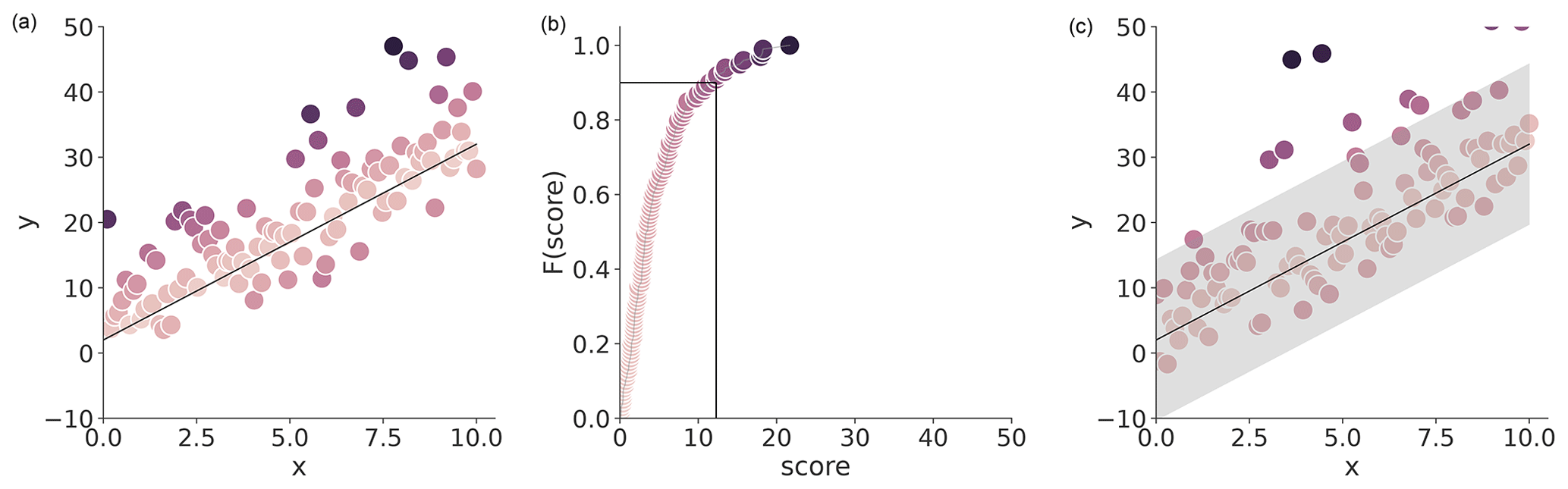
Figure 1Illustration of standard conformal prediction applied to a regression setting. (a) The black line shows the prediction of a model. The colored points show the real observation – the darker the color, the bigger the prediction residual, i.e., the non-conformity score. (b) CDF of the non-conformity score distribution and the respective cut-off quantile at α=0.1. (c) The prediction of μ, with the CP interval defined by the value on the cut-off quantile, based on the test data.
2.2 Uncertainty estimation models
This section introduces the models and metrics used to answer our research questions. We introduce HopCPT and its “global” variant, HopCPT-G, in Sect. 2.2.1 and 2.2.2, respectively. Section 2.2.3 presents CMAL.
2.2.1 HopCPT
Why are modeling systems often successfully used for decision-making even if they do not provide uncertainty predictions? We believe that this is because decision-makers implicitly consider the model behavior over time and compare a given forecast to the recent performance and the model behavior in similar situations. We thus design HopCPT (Auer et al., 2023) to explicitly capture this notion in a quantitative way.
HopCPT is the current state-of-the-art approach for conformal time series prediction. The uncertainty of time series data often varies heavily between certain periods. One reason is seasonal patterns. For example, for many alpine rivers, long-lasting periods of low flows in winter exhibit lower predictive uncertainty than large events in late spring, where glacier melt and convectional precipitation events interact. Another reason is the occurrence of irregular but recurring events such as those induced by torrential rain. Note that shifts also play an important role within events as their frequency and intensity can change over time. HopCPT addresses these challenges by viewing the time series as a soft partitioning of time periods, where each partition element exhibits individual uncertainty properties. We refer to such a set of time points as a regime (Quandt, 1958; Hamilton, 1990) and assume that one can identify them by the covariates and the lagged target of the time series. HopCPT learns to weight which past observations of the calibration data – i.e., calibration points – are likely to be from the same regime as the current point. We want to emphasize that, here and throughout the paper, the phrase “calibration data” refers to data that are not utilized in training the underlying point prediction model. This aligns with the conventional terminology in probabilistic applications in general and in the CP literature in particular.1 Based on this information, the different calibration points are weighted differently when constructing the prediction interval. Since the considered time steps in the interval calculation are from the same regime, one can assume that exchangeability is given and that, therefore, the validity of the prediction interval holds. Yet, since time points from unrelated regimes are disregarded, HopCPT results in tighter intervals than, for example, standard CP.
More formally, HopCPT assigns a weight to a past time step i∈M in the memory M given the current time step t. The weight reflects the similarity between the given time step i and the current time step t. Intuitively, we can say that the weight should be high when i is from the same regime as t and should otherwise be low. These weights are constructed with the modern Hopfield network component of HopCPT as follows:
where zi∈ℝd is the representation input for time step i, represents an encoding module, and and are learned weight matrices; β is a hyperparameter that represents the inverse of the so-called softmax temperature, which adjusts the sharpness of softmax-generated probability distributions (low temperatures push all the attention to a single value, while high temperatures distribute the attention uniformly). The model parameters of HopCPT are estimated using a standard gradient-based learning procedure, optimized with an MSE (mean square error)-like loss function. For the sake of completeness, Appendix D provides a more detailed review of the original loss function.
The weights form the basis for the weighted conformal prediction interval (Foygel Barber et al., 2022). Besides the weighting, HopCPT deviates from standard CP as it does not consider the one-sided quantile of the absolute errors (non-conformity scores) but instead follows Xu and Xie (2022a) and excludes the lower and upper quantiles of the relative errors. Formally,2 the prediction interval of time step t is calculated by
where Qτ is the τ quantile, and is a point mass distribution (i.e., a degenerate distribution where all the mass is concentrated at a single point) at the prediction error at time step i. This essentially means we compute the τ quantile across a mixture of M distributions, each corresponding to a distinct time step i in the memory, characterized by a point mass in relation to its prediction error ϵi. Thus, each of these distributions is concentrated at ϵi, with density 1 and 0 elsewhere.
HopCPT retrieves the calibration data points during the prediction from the modern Hopfield memory (Ramsauer et al., 2021) of the model. Thus, one can simply add every new and available observation to the memory. This corresponds to an automatic recalibration, which accounts for shifts in the data distribution. In addition, HopCPT allows us to add a so-called temporal encoding to the time steps. This encoding adds information about the time difference between the predicted time step and the previous time steps. Given this information, HopCPT can learn to weight recent points more highly, which further helps to address distribution shifts. This retrieval via the modern Hopfield memory is closely related to transformer attention (Vaswani et al., 2017, Appendix E).
HopCPT has already exhibited good performance in streamflow uncertainty prediction (Auer et al., 2023). In this work, we use HopCPT approach as a tool to explore the effects of data availability on uncertainty prediction.
Memory update. In Auer et al. (2023), HopCPT updates the Hopfield memory after each prediction with the – then – previous prediction error. However, this requires access to the target label of this time step to calculate the error of the prediction model. In streamflow modeling, we often do not have direct access to the target label (i.e., the streamflow measurement) before a new prediction has to be issued. Therefore, we adapt HopCPT to use a fixed memory that is only based on the calibration data by default. We refer to this adaptation as the “offline mode” in contrast to the original “online mode”. Given the notation from Eq. (3), this means that, in online mode, the memory M contains all time steps up to time step t−1, while, in offline mode, the memory is fixed per time series and only includes the calibration data.
In practice, one could expect that the memory may be updated intermittently whenever new data become available. Hence, we explore the influence of different updating schemes (Sect. 3.2).
Input features. Auer et al. (2023) concatenate (static and dynamic) time series covariates, model predictions, and lagged targets as input features to generate the representation zi of a time step i. However, the use of the lagged target requires access to the target label right after the prediction, which is typically not possible in streamflow prediction. A straightforward solution would be to simply exclude the lagged target as an input feature. However, since most current rainfall–runoff models follow a state-space approach, we also explore how a lack of labels can be compensated for by using the model state. We hypothesize that this state should include most of the relevant information that would have been provided by the streamflow observations, as well as additional information that is not available to HopCPT in the original publication. Note that (a) the model states potentially contain more information than just the model prediction because the prediction is some projection of its state3, and (2) the state likely encodes important historical information beyond the current time step. Figure 2 shows an example hydrograph of a random basin with the predictions of HopCPT.
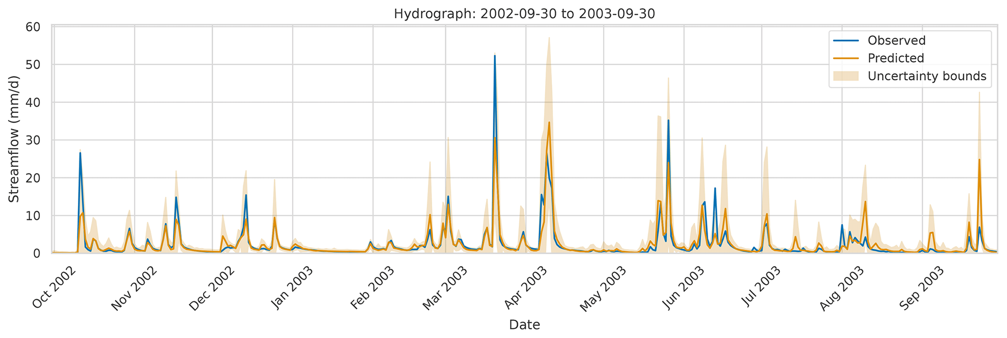
Figure 2The observed streamflow (blue), the prediction (gold), and HopCPT's prediction interval (light gold; offline mode and model states as input) for a random basin (ID no. 02077200) from October 2002 to October 2003. For the prediction interval, we set α=0.05. HopCPT generates wider prediction intervals where the prediction model is uncertain. Hence, it also covers the observed streamflow for values where the predicted and the real streamflows are quite different. In confident areas, the prediction interval is much narrower.
2.2.2 HopCPT-G
We hypothesize that the union of the existing calibration data represents not only the included streamflow time series but a general set of existing streamflow regimes. In this scenario, one could utilize the error information from similar situations in other basins to best model the current situation in a specific basin. This global information sharing could be especially beneficial if (calibration) data in individual basins are scarce. Further, the application to ungauged basins should be possible. In a simple case, where the error information is only relevant within a certain time series, HopCPT can learn to fall back to the local setting and only up-weight the calibration data of its own time series. To examine the potential of global memory, we modify HopCPT so that it operates based on global memory for both training and inference. We refer to this new model as HopCPT-G.
During inference, the association weights and prediction interval calculations of HopCPT-G are very similar to those of HopCPT. Equations (1) and (3) are still applicable; however, the memory M consists of all available time steps of all time series – in contrast to HopCPT, where only the time series of the predicted basin is used.
Figure 3 illustrates the difference. While, in HopCPT, only the learned weights are shared between different time steps, in HopCPT-G, both the learned weights and the memory vectors are shared between different time series.
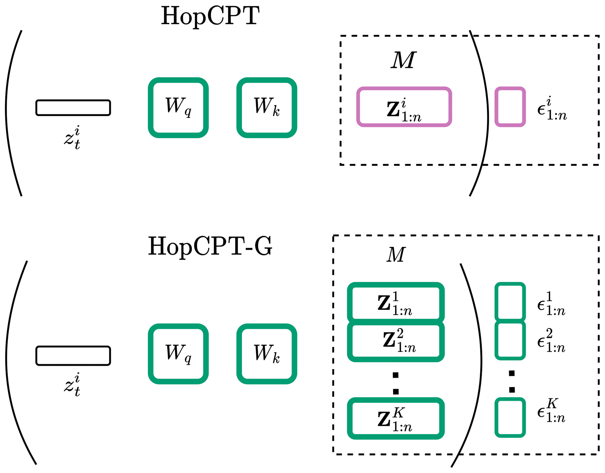
Figure 3Illustration of the difference between HopCPT and HopCPT-G. The shared weights and vectors are outlined in green, and the vectors that are specific to a specific time series are in magenta. HopCPT-G also shares the memory vectors and incorporates all available time steps.
This change is also reflected in the training loss. N time steps are drawn without replacement from K randomly selected time series. The loss for this batch is then calculated as
To ensure that the samples of our own time series (which are likely to be the most relevant) are in the batch, we choose N and K in such a way that all samples of the K series are in the batch.
PUB training. It is crucial for HopCPT-G to learn a time step representation which captures rich information about the error regime. As shown in multiple works, machine learning models often suffer from shortcut learning (Lapuschkin et al., 2019; Geirhos et al., 2020). For HopCPT-G, a potential shortcut might be just to learn to distinguish the different time series. This result would harm the PUB prediction performance in particular as it relies on representations which generalize over individual time series. To facilitate more robust representations that avoid this learning shortcut, we propose a training loss that masks out all observations of the time series to which the predicted time step belongs. In other words, HopCPT-G can only use the error observations from the other time series to form its prediction in the training phase. This way, the shortcut of only learning to consider its “own” time series is impossible. Formally, this changes the association matrix A to
where id maps a time step to an identifier of its corresponding time series.
2.2.3 CMAL
CMAL (Klotz et al., 2022) is an LSTM-based mixture density network (Bishop, 1994). The model predicts the parameters of asymmetric Laplacian distributions. This choice of distribution allows the modeling of asymmetric uncertainties that are typical for many hydrological variables. The direct comparison to HopCPT is slightly problematic as CMAL does not operate on top of an existing prediction model. However, as one of the best models for uncertainty estimation in streamflow prediction, CMAL is a good performance yardstick in our evaluation.
2.3 Metrics
The evaluation focuses on the validity and efficiency of the prediction intervals of the models. Validity means that, when a certain coverage, e.g., 90 %, is specified, 90 % of the test data are also actually covered by the prediction interval. This criterion is measured by the Δ Cov metric, which represents the difference between the specified and the empirical coverage. Δ Cov is, at best, zero, while a notably negative Δ Cov diminishes the utility of the model. A positive Δ Cov is less problematic but is a sign that the model could provide more efficient intervals. Here, efficiency refers to the width of the prediction interval: a more narrow prediction interval is more efficient than a wider one. We evaluate this property with the PI width metric, which simply corresponds to the average width of the prediction interval over the evaluation period. A smaller PI width value is therefore better. Additionally, we evaluate the Winkler score, which jointly elicits both criteria and thus allows an easy comparison between different models. The Winkler score is calculated as
The score corresponds to the interval width whenever the observed value yt is within the interval of – otherwise, the score gives a penalty that is weighted by the warranted coverage level α.4 The Winkler score as such is calculated for each individual time step t, but we report the average over all time steps and basins (as is common in time series literature).
Experiment I, II, and III address the respective research questions of this paper. In addition, we conduct a performance comparison of different uncertainty models in Appendix B. Specifically, we compare HopCPT with CMAL (Klotz et al., 2022), Bluecat (Koutsoyiannis and Montanari, 2022), and a kNN-based approach (Wani et al., 2017; Auer et al., 2023). We evaluate all approaches based on the predictions of an LSTM-based rainfall–runoff model with three coverage levels: . Appendix G provides the technical details of our experimental setup, and Appendix H describes our hyperparameter search.
3.1 Data
All experiments are based on the public Catchment Attributes and Meteorology for Large-Sample Studies (CAMELS) dataset (Newman et al., 2015; Addor et al., 2017a). CAMELS comprises basis-averaged daily meteorological forcings derived from three different gridded data products across the United States of America. We used the same 531 basins which were used in the original benchmark (Newman et al., 2017) and in related follow-up work (Kratzert et al., 2019a; Klotz et al., 2022). This subset contains basins ranging in size from 4 to 2000 km2. The dataset contains daily meteorological forcings (precipitation, temperature, shortwave radiation, humidity) from three different data sources (NLDAS, Maurer, DayMet); daily streamflow discharge data from the US Geological Survey; and basin-averaged catchment attributes related to soil, geology, vegetation, and climate. The dataset is split into three parts across the time axis. These parts represent (1) the training data for the prediction model, (2) the calibration data used by the uncertainty model, and (3) the test data for evaluation. For CMAL, which does not need any calibration data, both the training and calibration split are used for training.
3.2 Experiment I
This experiment assesses how recent measurements affect the performance of HopCPT. We split it into two parts.
Experiment I-a compares identical HopCPT models once with offline memory and once with online memory (see Sect. 2.2.1). We examine two different input feature configurations – one using the time series covariates and the model prediction and one using the model state and model prediction (see Sect. 2.2.1). In addition to the quantitative comparison, we qualitatively analyze the individual time series for which the performance gap between online and offline is the greatest. This yields insights into potential shifts in the prediction error in such cases.
Experiment I-b analyzes intermediate memory update strategies that fall between fully offline and fully online. In real-world scenarios, gathering the labels with some delay might sometimes be feasible and at least partially help to mitigate the impact of distribution shifts. Therefore, we evaluate HopCPT with a memory update frequency of 1 week, 1 month, 3 months, 6 months, 1 year, and 2 years (note that the sampling frequency of the series is 1 d, and the overall test period is 9 years) and compare the results to the offline and fully online models (i.e., frequency of 1 d).
3.3 Experiment II
In Experiment II, we investigate how much the data from a given basin contribute towards the uncertainty predictions for said basin itself. We do so by first comparing HopCPT with HopCPT-G in a gauged setting (Experiment II-a) and then comparing HopCPT-G with CMAL in an ungauged setting (Experiment II-b). The details for both comparisons are explained in the following.
Experiment II-a compares HopCPT-G to the originally proposed HopCPT in the gauged setting. We focus on the HopCPT feature configuration which includes the model state and prediction as we hypothesize that this configuration is less likely to simply down-weight samples from time series that are different from the predicted one. We additionally evaluate HopCPT-G with PUB training, i.e., the adapted training loss (see Eq. 6). Although we do not evaluate on ungauged basins in this setting, PUB training can increase the tendency of HopCPT to incorporate data from other basins – and that could potentially lead to more robust representations.
Experiment II-b investigates if uncertainty estimates are also possible without any local information from the predicted basin. To examine this scenario, we loosely follow the PUB setting from Kratzert et al. (2019a): the set of time series is split into 11 mutually exclusive subsets of equal size. The principle is similar to k-fold cross-validation (but not on a per-sample basis): we define that for the kth fold; the gauged basins are the union of all but the kth subset, while the kth subset represents the ungauged basins. We reserve one of the folds for hyperparameter tuning and exclude it from the evaluation. For the other 10 folds, we individually train the prediction and uncertainty model on the gauged basins (9 out of 10 subsets) and evaluate them based on the ungauged basins from the remaining subset. Note that, within each subset, each time series is (as in the standard case) split into training, calibration, and test data. CMAL's training data encompass both the training and calibration split to ensure that, in total, each model has the same amount of data available. We evaluate only the test period of the ungauged basins (this avoids information leakage from the training and calibration periods of the gauged basins). We evaluate two variants of HopCPT: (1) HopCPT-G with normal training and (2) HopCPT-G with PUB training. For both variants, we use the model state and prediction as input features.
3.4 Experiment III
Experiment III examines the uncertainty estimation for peak flows specifically. Peak-flow uncertainties are especially hard to capture. Firstly, because prediction models tend to make larger errors (i.e., high aleatoric uncertainty) and, secondly, because the occurrence of peak-flow events is limited (i.e., high epistemic uncertainty). To measure the respective performance, we calculate the metrics only using time steps where the streamflow observations are in the top x % of the corresponding basin. Specifically, we evaluate for (and 100 comprises all data and hence corresponds to the standard evaluation) within the gauged-basin setting of Experiment II. For the sake of completeness, Appendix J3 also presents the peak-flow evaluation for the other experiments.
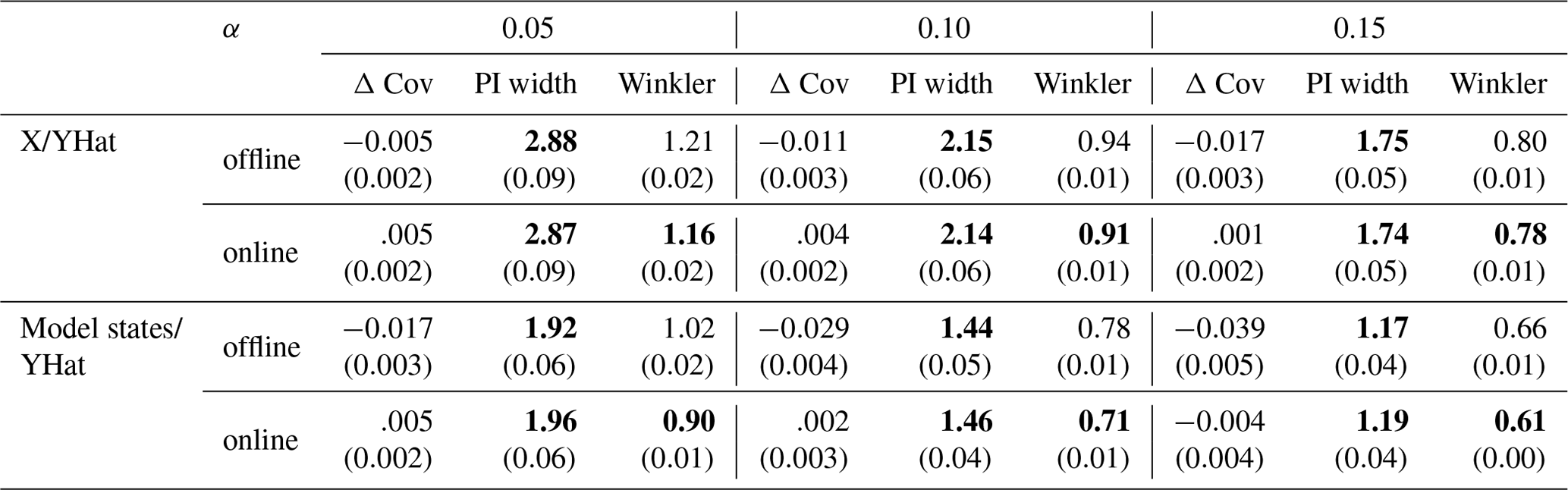
Table 1HopCPT performance of the two evaluated input combinations in offline and online mode for the mis-coverage levels . The values represent the average over all basins. Bold numbers correspond to the best result for the respective metric in the experiment (PI width and Winkler score); the significance is tested with a Mann–Whitney U test at p<0.005. For PI width and Winkler score, lower values are better – for Δ, Cov non-negative values close to 0 are best. The values in parentheses represent the standard deviation over the different seeds.
4.1 Experiment I
Experiment I-a compares the offline and online modes of HopCPT. Table 1 shows that the main performance advantage of the online setting is its better coverage. This holds especially true for the HopCPT variant, which uses the model states as features. The width of the prediction interval stays almost constant between offline and online approaches. This suggests that the change in Winkler score is a direct effect of the lower or higher coverage. We argue that the slight loss in coverage for the offline setting is due to a distribution shift in some basins (Fig. 4): while the coverage distribution of the basins with the highest coverage is very similar between the offline and online cases, the biggest change happens in the 10 %–20 % of basins with the lowest coverage.
A particularly striking examples of this shift is shown in Fig. 5: in the prediction year 2000 (approximately 1 year after the memory end), the offline setting provides reasonable intervals. However, in the year 2004, the real streamflow seems to be shifted upwards for low flows and downwards for some higher flows. Since the output of the prediction model remains roughly constant, we suggest that the phenomenon at hand is a shift in the runoff that is not visible in the input patterns. The online model can accommodate for this shift since the new information (in the form of the shifted observations) are incorporated into the memory. The offline model simply has no mechanism to account for that and to construct invalid intervals. Figures J1 and J2 in the Appendix show additional examples of this error shift behavior.
Experiment I-b investigates the effect of HopCPT with infrequent memory updates as intermediate settings between the edge cases of fully online and offline settings. Table 2 presents the results. The slight coverage loss increases gradually with a higher update delay – as illustrated in Fig. 6. However, an update frequency of 1 year already halves the coverage loss compared to the offline setting. The changes in the PI width are less clear and non-monotonic; however, the variation is negligible anyway.
Regarding the answer to RQI (does up-to-date information improve the general uncertainty estimation?), our results indeed suggest that a continuous incorporation of new data improves uncertainty predictions. For the center of the predictive distribution (associated with large α values; Table 1), our results are less pronounced than for the tails (associated with small α values; Table 1). Further, continuously updating the uncertainty estimates as new data come along is very useful, given that environmental processes are associated with all kinds of distribution shifts. In our experiments, a memory update mechanism was advantageous even in cases where real-world constraints only allow for very infrequent updates (Table 2).
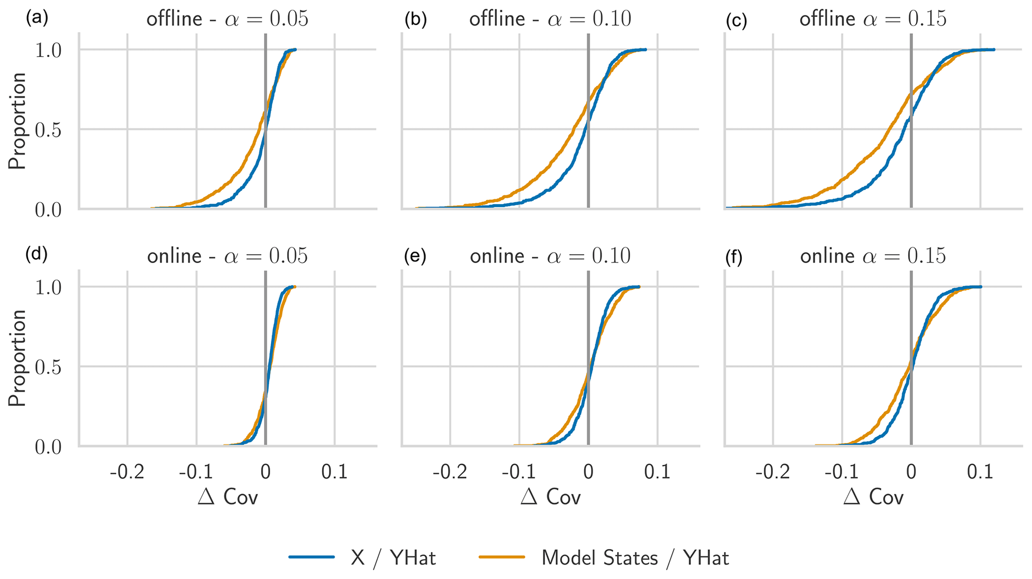
Figure 4CDF of Δ Cov over individual basins for the models evaluated in Experiment I-a. Panels (d–f) show the results for the online mode, i.e., where the memory gets updated after each prediction, and panels (a–c) show the results for the offline mode, i.e., where the memory does not get updated during the test period. For Δ Cov, non-negative values close to 0 are best.
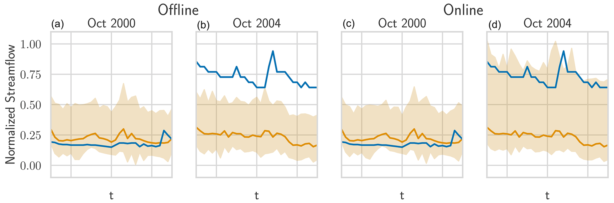
Figure 5The real streamflow (blue), the prediction (gold), and HopCPT's prediction interval (light gold) for a basin (ID no. 12447390) in October 2000 and October 2004. The two plots on the left show HopCPT in offline mode, and the two plots on the right show HopCPT in online mode. The online mode allows HopCPT to account for the distribution shift in October 2004.
Table 2Performance of HopCPT with different memory update behaviors for the mis-coverage levels . The “delay” column indicates the update frequency of the memory. The values represent the average over all basins. Bold numbers correspond to the best result for the respective metric in the experiment (PI width and Winkler score). For PI width and Winkler score, lower values are better; for Δ Cov, non-negative values close to 0 are best. The values in parentheses represent the standard deviation over the different seeds.
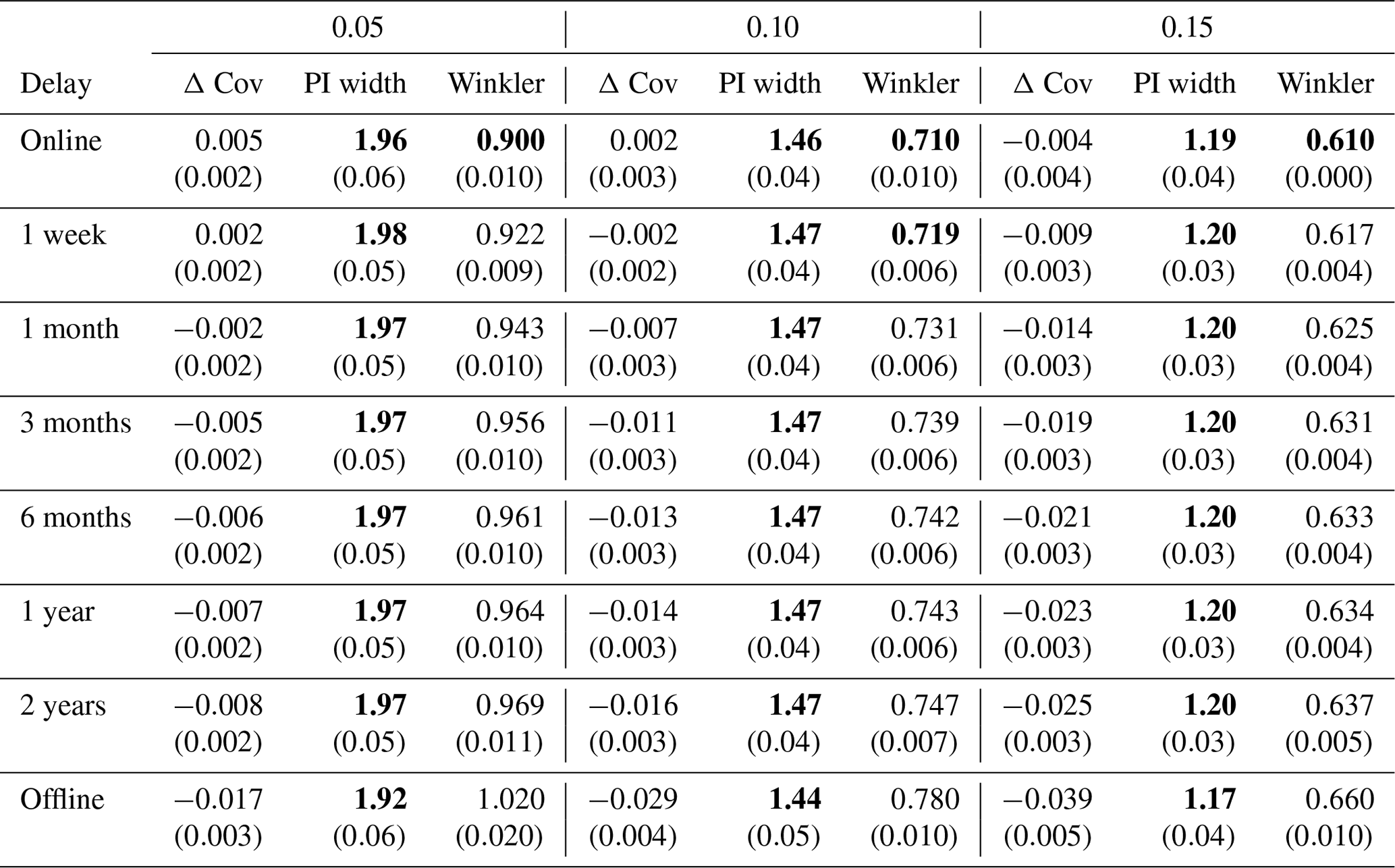
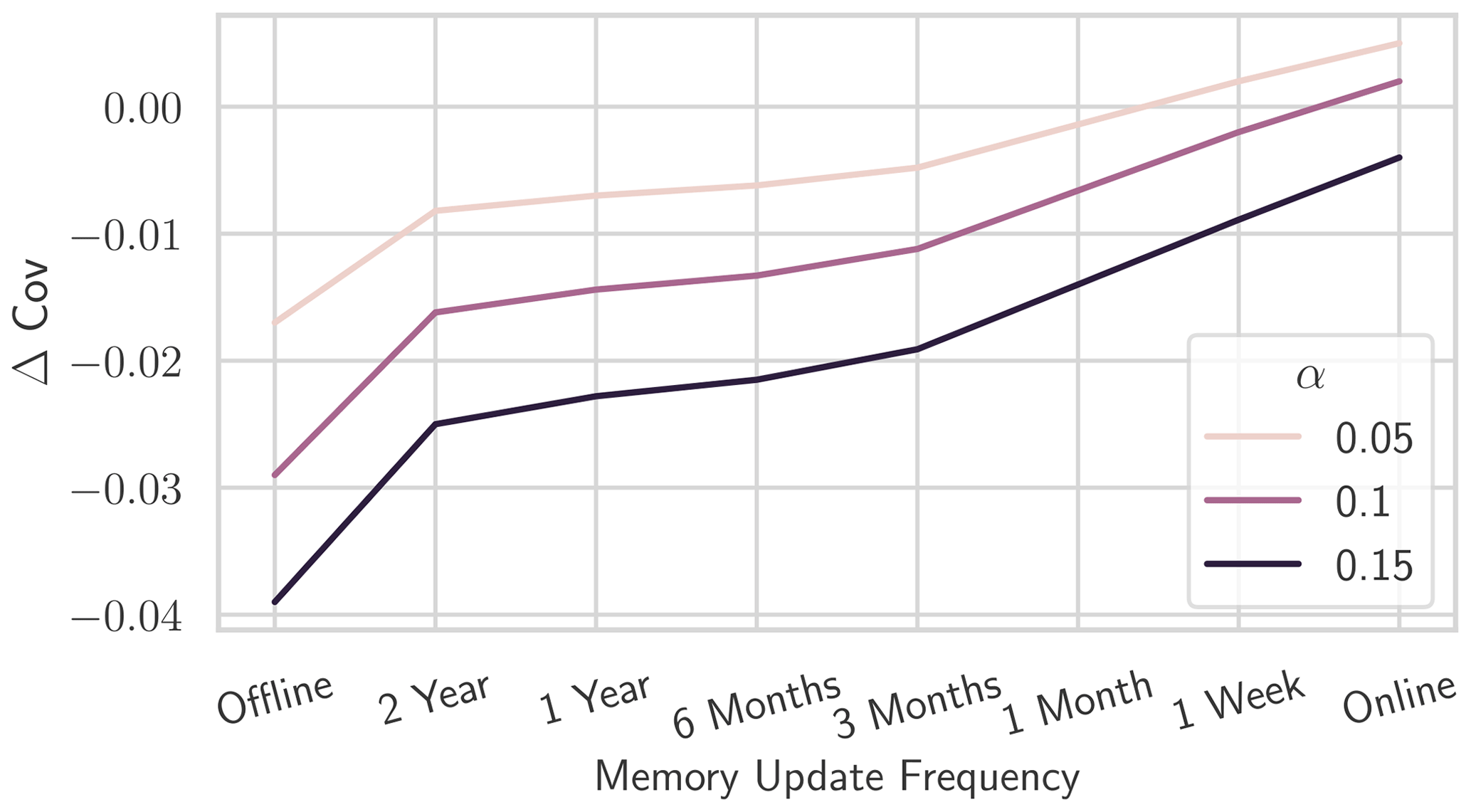
Figure 6Δ Cov of HopCPT for different memory update frequency settings. Increasing update frequency monotonically improves the coverage for each evaluated coverage level. For Δ Cov, non-negative values close to 0 are best.
4.2 Experiment II
Experiment II-a probes the effect of global data in the gauged-basin setting. Table 3 shows the result of HopCPT-G (with and without PUB training) and compares it to the non-global HopCPT. Surprisingly, the shared memory of HopCPT-G (no PUB training) does not improve the results. However, it also does not do any notable harm. We hypothesize that the calibration data of each basin are already so comprehensive that all relevant error regimes for the respective basin are covered with sufficient resolution. The slight degradation in performance could result from either (i) the additional challenge of learning to disregard all non-relevant basins or (ii) the missing temporal encoding in HopCPT-G. The PUB training procedure, on the other hand, notably improves the coverage. However, this improvement comes at the cost of efficiency. Hence, the resulting Winkler score is similar to that of the other approaches.
Figure 7 shows the coverage distribution over the individual basins. The distributions of HopCPT and HopCPT-G are very similar. This indicates that HopCPT-G cannot profit from the cross-time-series information but successfully learns to exclude irrelevant basins in order to arrive at the right error distribution.
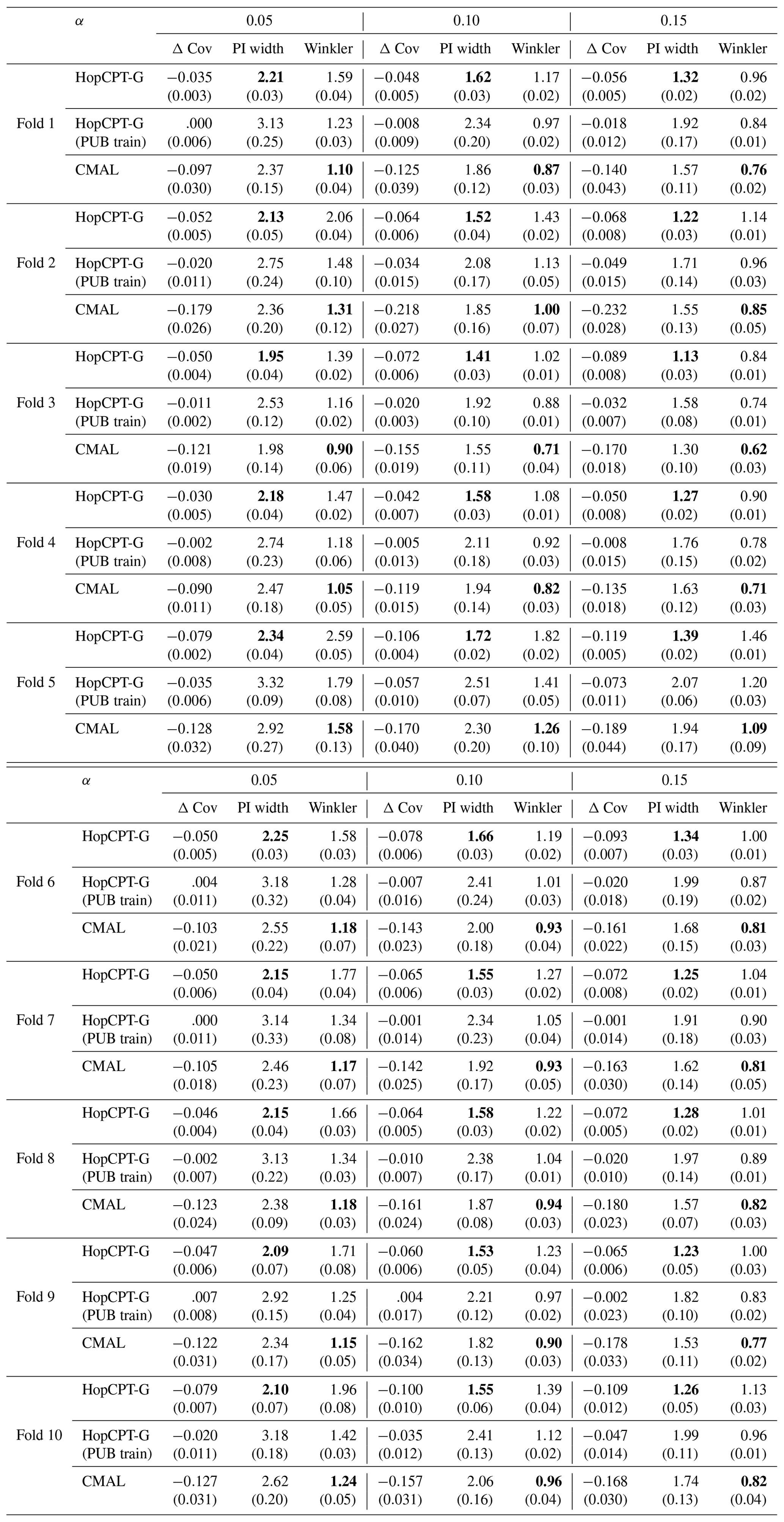
Experiment II-b investigates the PUB setting. Table 4 shows the result of the evaluation. CMAL, which has very good coverage in a gauged-basin setting (see Appendix B), exhibits a noticeable under-coverage. HopCPT-G, on the other hand, only slightly loses coverage compared to the non-PUB setting. HopCPT-G with PUB training reduces the coverage loss notably. Its efficiency is comparable to CMAL and HopCPT-G. CMAL achieves the best Winkler score despite its high under-coverage. This suggests that the uncovered samples are relatively close to the border of the prediction interval. Figure 8 shows the distribution of Δ Cov over the individual time series. Since the PUB setting does still yield acceptable performances but does not allow us to use information from a given basin, one can conclude that the global setting is able to transfer uncertainty information about the uncertainty from other basins to the unseen basins. Quantitative metrics for the individual folds can be found in the Appendix in Table J1.
Regarding the answer to RQII (are the data from a given basin required to get good uncertainty estimates?), our result suggests that local information is beneficial for efficient uncertainty intervals. Given that enough local information is available and the average quality of the estimate is the focus (in contrast to RQIII), it is also sufficient to provide reasonable uncertainty estimates (Experiment II-a). However, local information is not strictly necessary to produce sensible uncertainty estimations, and information transfer via global information is possible (Experiment II-b).
Table 3Performance of the different HopCPT variants for the mis-coverage levels . The values represent the average over all basins. Bold numbers correspond to the best result for the respective metric in the experiment (PI width and Winkler score); the significance is tested with a Mann–Whitney U test at p<0.005. For PI width and Winkler score, lower values are better; for Δ Cov, non-negative values close to 0 are best. The values in parentheses represent the standard deviation over the different seeds.
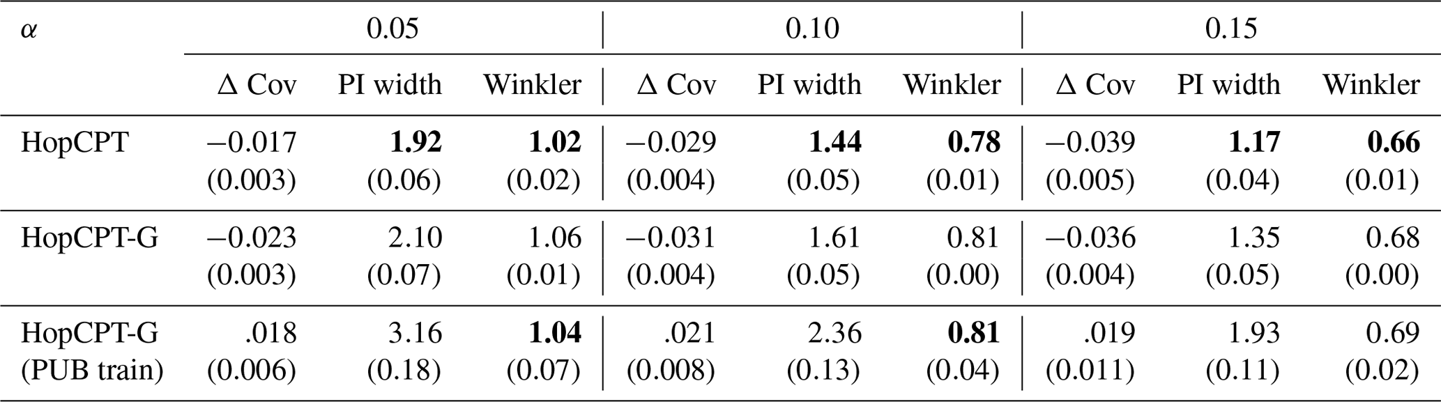
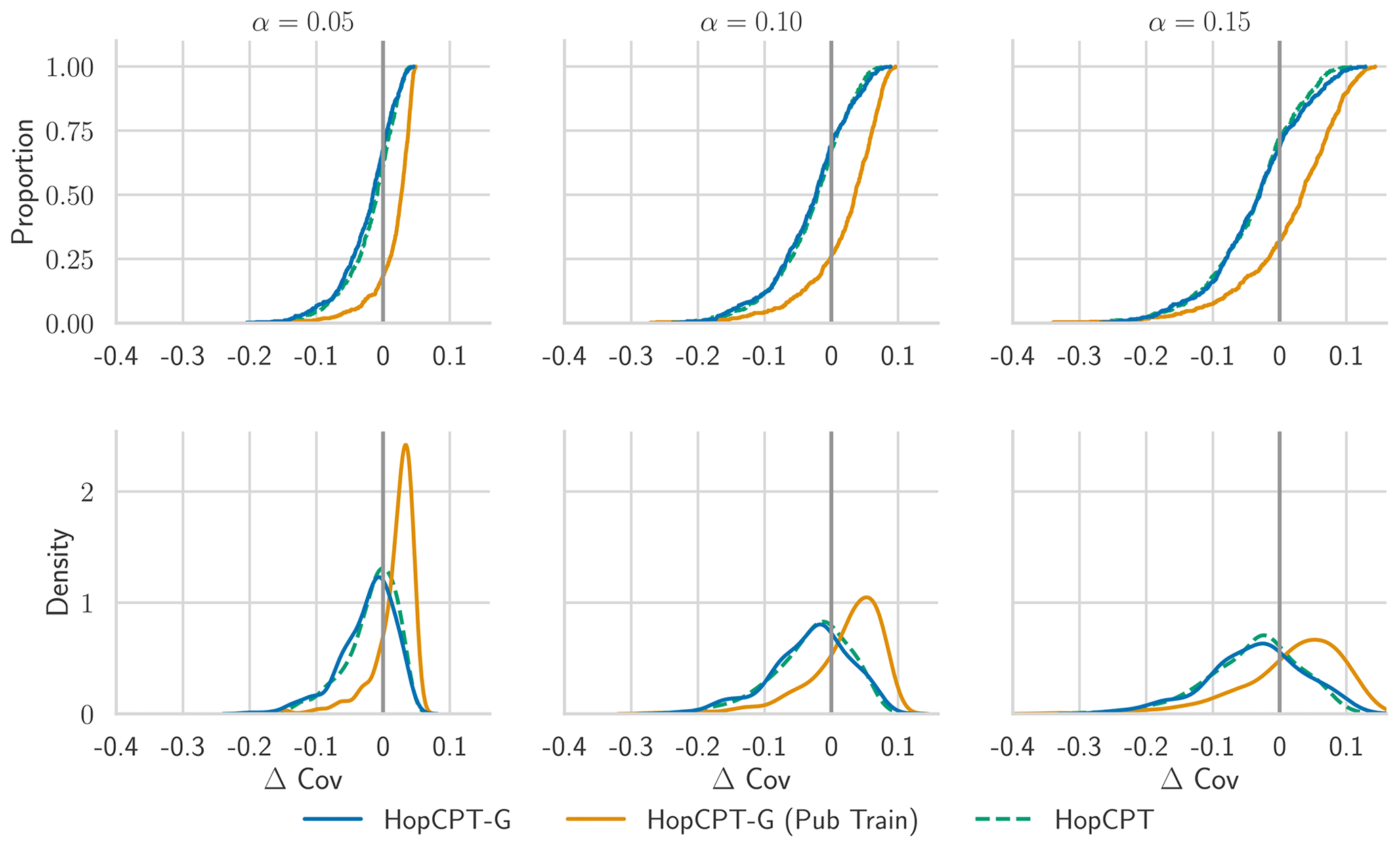
Figure 7CDF and PDF of Δ Cov over individual basins for models evaluated in Experiment II-a. For Δ Cov, non-negative values close to 0 are best.
Table 4Performance of different models in the PUB experiment for the mis-coverage levels . The values represent the average over all test basins of all splits. Bold numbers correspond to the best result for the respective metric in the experiment (PI width and Winkler score); the significance is tested with a Mann–Whitney U test at p<0.005. For PI width and Winkler score, lower values are better; for Δ, Cov non-negative values close to 0 are best. The values in parentheses represent the standard deviation over the different seeds.
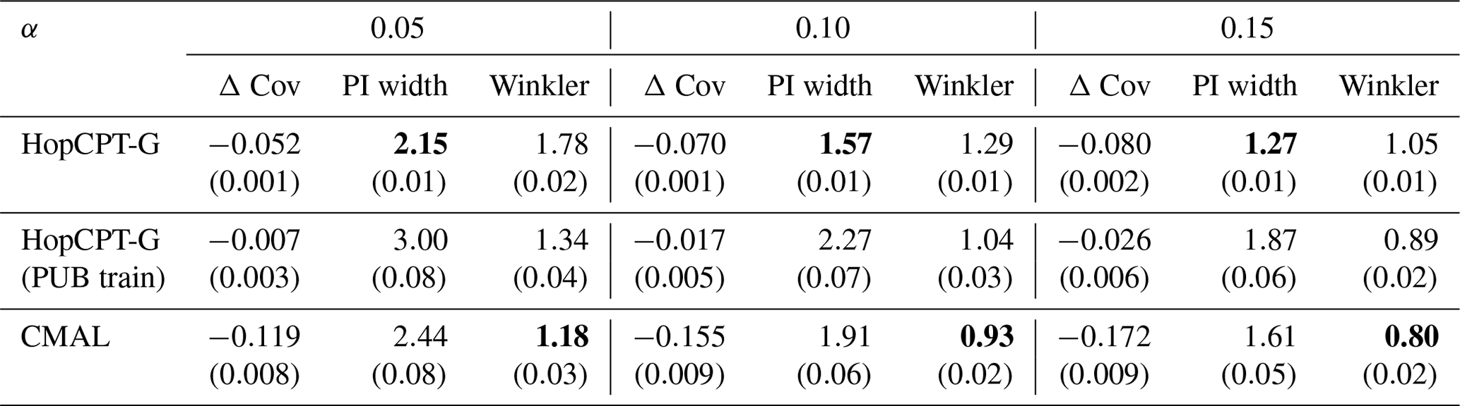

Figure 8CDF and PDF of Δ Cov over all individual test basins of all PUB folds for models evaluated in Experiment II-b. For Δ Cov, non-negative values close to 0 are best.
4.3 Experiment III
In contrast to our results from Experiment II, the peak-flow performance exhibits a notable difference between the HopCPT variants (Fig. 9). HopCPT-G provides better coverage than HopCPT, and PUB training boosts this further. The coverage difference between the HopCPT variants also increases with increasing α. CMAL, which is also a fully global model, achieves the best Winkler scores in the peak-flow setting. This indicates that the information from other basins is beneficial for peak-flow regimes – even when plenty of past information for the basin is available. We argue that this is because the data are more scarce in these regimes, and certain situations might not be available in the observed past of the individual basin. Thus, in this situation, it becomes useful to leverage information from the other basins in order to obtain good uncertainty estimates (we note that this is in contrast to the results from Experiment II, which showed that, for the average runoff predictions, no improvement is obtained by considering global information).
Regarding the answer to RQIII (are data from a single basin enough to get good uncertainty predictions for peak flows?), our results indicate that using only data from a single basin – that is, only considering the local information – leads to worse uncertainty estimates for peak-flow settings. The more restricted the peak-flow categorization that is chosen, the more pronounced this effect gets (Fig. 9). Using global information – i.e., information from other basins – improves the uncertainty estimates. In particular, this holds in terms of the reliability of the estimate (i.e., coverage).
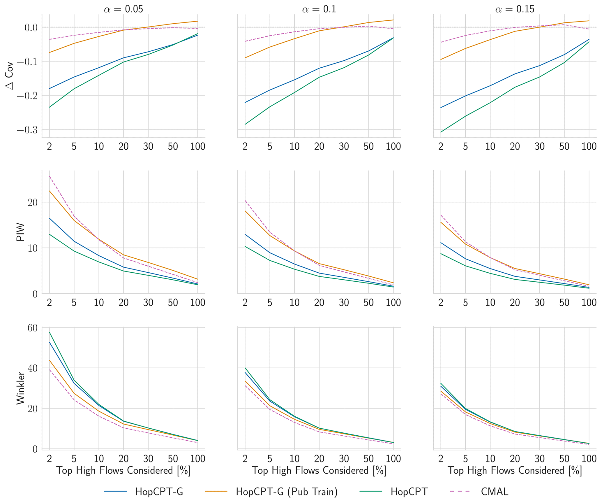
Figure 9Evaluation metrics for Experiment III. Only peak-flow time steps – defined via varying the share of the overall steps (x axis of the plots) – are considered for the respective metric. For PI width and Winkler score, lower values are better; for Δ Cov, non-negative values close to 0 are best.
This contribution investigates how the temporal (recency) and spatial (local vs. global) dimensions of information impact the quality of uncertainty estimates. To conduct our study, we apply the conformal prediction (CP) framework in the form of the Hopfield conformal prediction for time series (HopCPT) approach, which extends the CP framework for time series predictions. In short, we find that (a) the inclusion of the most recent information has notable benefits for the general uncertainty predictions, and (b) global information is not important for general uncertainty predictions but is pivotal for the provision of good bounds for peak flows.
Regarding (a), our analysis suggests that incorporating recent information helps to improve the uncertainty estimates. This is even true if the information can only be provided after longer periods (e.g., when, for technical reasons, only yearly updates are possible). We could qualitatively link this phenomenon to distribution shifts that appear over time. We conclude that continuous monitoring and incorporation of the newly obtained data in the prediction process are vital components of prediction systems that strive to provide reliable and efficient uncertainty estimations.
Regarding (b), our results indicate that local information is sufficient to provide good uncertainty estimates on average (assuming that a reasonable history over multiple years is provided). However, for peak flows, it is not. We argue that this is because the estimation problem is particularly hard since high-flow situations are diverse, have a high measurement variance, and happen very infrequently. Global information is able to improve the estimates. These observations are in accordance with the results from Frame et al. (2022) and Bertola et al. (2023), which indicate that the signals from different basins can be leveraged to make better predictions for peak flows. This can be taken to the extreme for predictions in ungauged basins. Indeed, our experiments in this regard suggest that reasonable uncertainty estimates can also be provided without any local information. However, whenever global information is used for uncertainty estimation, it is especially important that the respective model can selectively consider the relevant information – i.e., it can decide which parts of the overall information should be used for the current estimation. HopCPT-G and CMAL are both able to do that.
In future work, experiments with more scarce local data could reveal further advantages of approaches that incorporate global information. More broadly, CP offers a fresh perspective to uncertainty-aware streamflow prediction. Appendix C shows a first exploration of how the principles from CP can improve existing hydrological uncertainty estimations with minimal interventions. In the future, we want to explore how ideas from CP are able to refine other (perhaps less formal) approaches that are currently used in practice. Experiments with input perturbation techniques could give orthogonal insights into how different input features impact the uncertainty estimates of the models.
The Appendix is structured as follows: Appendix B compares the overall performance of different uncertainty methods, including HopCPT and CMAL. Appendix C investigates the impact of applying the principles of CP to the existing uncertainty estimation method Bluecat. Appendix F investigates how different input features influence the uncertainty estimation performance – i.e., provides an orthogonal dimension to the spatial and temporal consideration of the main paper. Appendices G and H provide details about the experimental setup and the hyperparameter tuning, respectively. Appendix I presents the point prediction metrics of the experiments. Finally, Appendix J provides additional results from the experiments in the main paper.
This section compares the performance of the different (non-global) methods5. For HopCPT, we evaluate the model in offline mode (i.e., without updating the memory as outlined in Sect. 2.2.1). Two variants for the input features are examined: (1) the time series features and the model prediction, similarly to the original work but without the lagged target, and (2) the model states and prediction as proposed in Sect. 2.2.1. For Bluecat, we selected the best model considering both the original Bluecat and the adapted version suggested in Sect. C. We follow Auer et al. (2023) and also evaluate against kNN as a naive similarity-based baseline (see Appendix B1). While Auer et al. (2023) show that the kNN on the time series features is not sufficient, we analyze the performance of kNN with (1) the model states and prediction (corresponding to HopCPT) and (2) only the model prediction (corresponding to Bluecat) as input. Additionally, we evaluate CMAL as the current state-of-the-art approach.
B1 kNN as naive similarity approach
HopCPT uses the similarity representation that is learned by the modern Hopfield network (MHN). A more naive way to consider such a similarity would be to simply use a kNN model based on the model inputs. Following the original work, we use such a kNN model as a baseline in the experiments. In hydrology, this approach was already proposed as an uncertainty estimation technique for streamflow prediction by Wani et al. (2017) and showed reasonable performance.
B2 Model intercomparison – results
Table B1 shows the evaluation of the different models. CMAL, closely followed by HopCPT, provides the best coverage at all coverage levels. While HopCPT with the model states and input reaches the most efficient – i.e., smallest – prediction intervals, CMAL performs best in terms of the Winkler score. This is slightly surprising, given that the Winkler score encompasses the coverage and PI width. However, the fact that Winkler score additionally considers the distance of the uncovered test samples leads us to the hypothesis that CMAL, as it is optimized to maximize the likelihood of all samples, results in smaller distances in that regard. In contrast, HopCPT and Bluecat do not consider the uncovered samples in optimization and calibration. The comparison between the HopCPT evaluations with different input features shows that adding the model states as inputs enhances the efficiency of HopCPT while keeping an approximate coverage, which results in an overall lower Winkler score. A more detailed analysis of the effect of different input modalities is given in Appendix F. The best variant of Bluecat falls behind HopCPT and CMAL in all three metrics. The kNN model, as a naive similarity measure baseline, also results in high under-coverage when considering the model states. This reinforces the motivation for a learned similarity measure, as already mentioned in the original HopCPT paper.
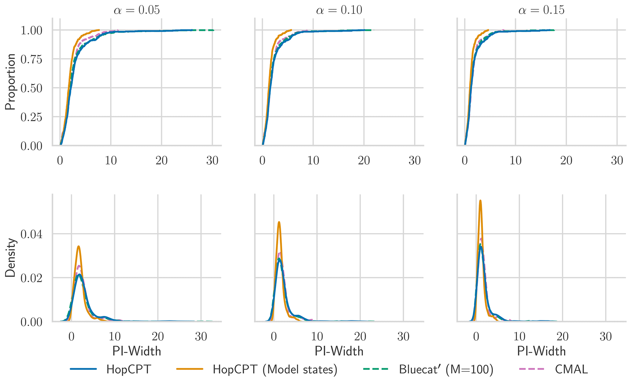
Regarding individual basin analysis, Fig. B1 gives more detailed insights into how the metrics are distributed around the individual basins. CMAL, which archives the best overall coverage, does not provide better coverage for all basins, but the high mean is driven by the higher over-coverage of the upper half of basins. This aligns with the analysis in Klotz et al. (2022). Overall, the coverage distribution of HopCPT is more centered around zero and better bounds the lowest coverage. As the cumulative distribution plot in Fig. B2 shows, for the 50 basins with the worst coverage (approximately 10 % of all basins), HopCPT without model states performs best, and the worst coverage is best for HopCPT (no matter if it is with or without model states). The distribution of the PI width (Fig. B3) is similar for all models; however, the efficiency advantage of HopCPT is most pronounced for the basins with larger prediction intervals.
Table B1Performance of the evaluated models for the mis-coverage levels . The values represent the average over all basins. Bold numbers correspond to the best result for the respective metric in the experiment (PI width and Winkler score), given that Δ Cov , i.e., given that the specific algorithm reached reasonable coverage (the result are displayed in italics otherwise); the significance is tested with a Mann–Whitney U test at p<0.005. The values in parentheses represent the standard deviation over the different seeds (results without these are from deterministic models).
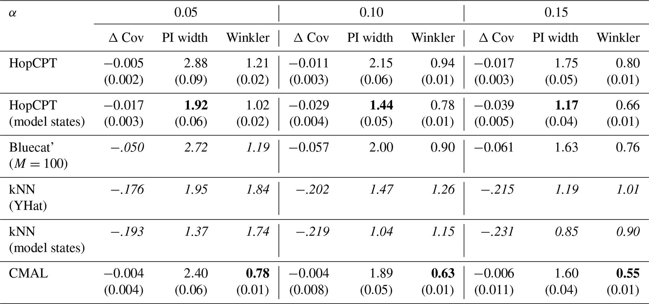
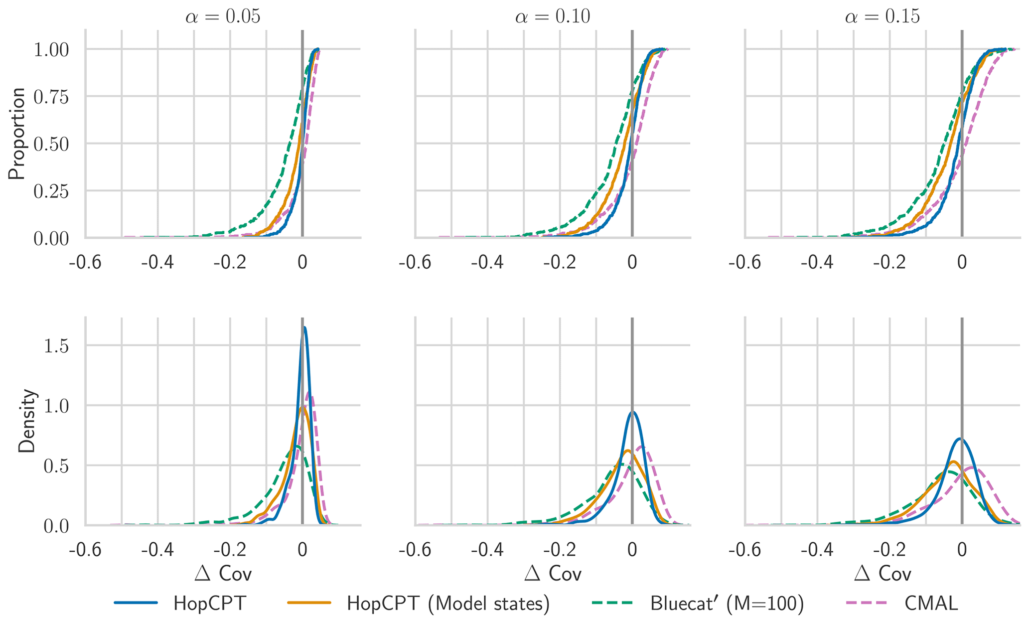
Figure B1CDF and PDF of Δ Cov over individual basins for models with approximate average coverage (Δ Cov ), as evaluated in Appendix B.
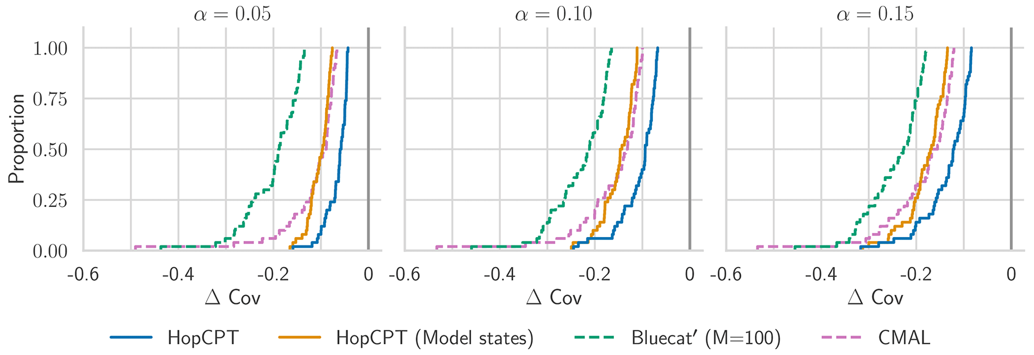
Figure B2CDF of Δ Cov over the 50 basins with the highest mis-coverage for models with approximate average coverage (Δ Cov ), as evaluated in Appendix B.
Similarly to HopCPT, the hydrological uncertainty estimation approach Bluecat (Koutsoyiannis and Montanari, 2022) aims to provide a prediction interval given a point prediction model and a set of data points (calibration data). Bluecat first evaluates the calibration data. Then, for a new prediction point, the calibration point with the most similar model prediction and all points within a certain distance to this point are considered. This can be seen as a special form of kNN where (1) the distance metric between two points is the distance of the model predictions and where (2) not only k points but all points within a certain distance threshold are considered (Rozos et al., 2022). Given this set of selected calibration points, similarly to the CP framework, the specified quantiles are calculated and provide the bounds of the confidence band.
C1 The CP perspective on Bluecat (Bluecat')
Viewing Bluecat through a CP lens suggests a relatively low-effort improvement in the form of the introduction of a calibration set for the interval prediction. Bluecat only uses the training data of the prediction model to determine the prediction interval; i.e., prediction training data equate to calibration data. However, the CP literature suggests that an independent calibration set can give a more unbiased estimate since prediction models can easily overfit training data (and, as a result, the prediction intervals might be overly optimistic and therefore might not fulfill the specified coverage criterion). We refer to this adaptation as Bluecat' throughout the paper.
We evaluate Bluecat once as originally proposed (Bluecat) and once with the adaption (Bluecat'). Bluecat requires setting the hyperparameter M, which controls how many close data points are considered. In the original publication, there is no clear guidance on how to select the parameter for new datasets, which is why we evaluate two variations: (1) tuning the hyperparameters with the same model selection criteria as in HopCPT (resulting in M=225) and (2) using the hyperparameter value from the original publication (M=100).
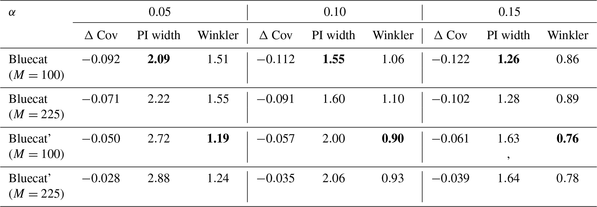
C2 Bluecat – results
Table C1 shows the results of the comparison. The adaptation Bluecat' achieves considerably improved coverage. The lower Winkler scores further indicate the overall better performance of Bluecat'. These results support the hypothesis that Bluecat intervals are overly optimistic since they are based on the – most likely overfitted – training-data predictions of the prediction model. Further, the hyperparameter-tuned versions (M=225) of both Bluecat variants enhance the coverage of the models at the cost of lower interval efficiency. This makes sense as the model selection favors models with better coverage as long as no model fully achieves the specified coverage.
Table C1Performance of the evaluated Bluecat variants for the mis-coverage levels . The values represent the average over all basins. Bold numbers correspond to the best result for the respective metric in the experiment (PI width and Winkler score). As Bluecat is deterministic, no standard deviation is given.
Auer et al. (2023) propose a gradient-based learning procedure that utilizes a loss function that is based on the mean squared error (MSE). The specific loss function ℒ is defined as follows:
where is a matrix representing the association weights between each pair of time steps in a time series with T points.6 The diagonal elements of , which correspond to the weights from a time step in relation to itself, are set to zero (masked out). ϵ1:T is a vector of the prediction error of the T points. For HopCPT-G, we propose an adapted version of this loss (see Sect. 2.2.2).
HopCPT employs a modern Hopfield network (MHN) to retrieve similar calibration points. MHNs are closely related to transformers (Vaswani et al., 2017) through their association and attention mechanisms. In fact, Ramsauer et al. (2021) show that the transformer attention is a special case of the MHN association, at which we arrive when the queries and keys are mapped in a certain way and given a specific inverse softmax temperature. However, the framework of MHN highlights the associative memory mechanism as HopCPT directly ingests encoded observations. This associative mechanism allows HopCPT to retrieve error information from situations that are similar to the given one. In the global variant (HopCPT-G), this even allows us to draw from the error information of different basins. MHNs further have the advantageous properties of exponential storage capacity and one-step update retrieval (Ramsauer et al., 2021).
This section assesses how different HopCPT inputs affect its performance. The experiment compares all combinations of the three potential feature components: time series covariates (X), model prediction (YHat), and model state. We use an LSTM prediction model. Hence, the model state refers to the two internal state vectors of the LSTM, which are updated in each new step and are – together with the current input – the basis for the output of the model. Specifically, we consider the state vectors right after the prediction since these states already consider the current input features. We tuned hyperparameters individually for each feature set combination. Additionally, we analyze results where we include the lagged target (Y) as a feature, as in the original HopCPT paper.
Table F1 shows the performance of HopCPT with the different input feature configurations. Interestingly, only using the time series covariates results in the best coverage. However, the prediction intervals in these settings are rather large, which is also reflected in notably higher Winkler scores. Therefore, we argue that using the model states as input features is indeed beneficial. This argument is further strengthened by the results in Sect. 4.1, where we see that the coverage loss is likely due to distribution shifts. Accounting for this shift by updating the memory leads to almost perfect coverage for the model state setting and unnecessary over-coverage in the covariate-only setting. Adding both the model prediction and the model state provides additional information. The model state does not only include information about the current covariates but also includes history information due to the recursive nature of the LSTM. The model prediction, on the other hand, can be seen as a projection of the model state where some relevant information could be lost. Extending the model state with additional inputs hardly changes the performance of HopCPT, which supports the hypothesis that the model state already includes the vast majority of the required information.
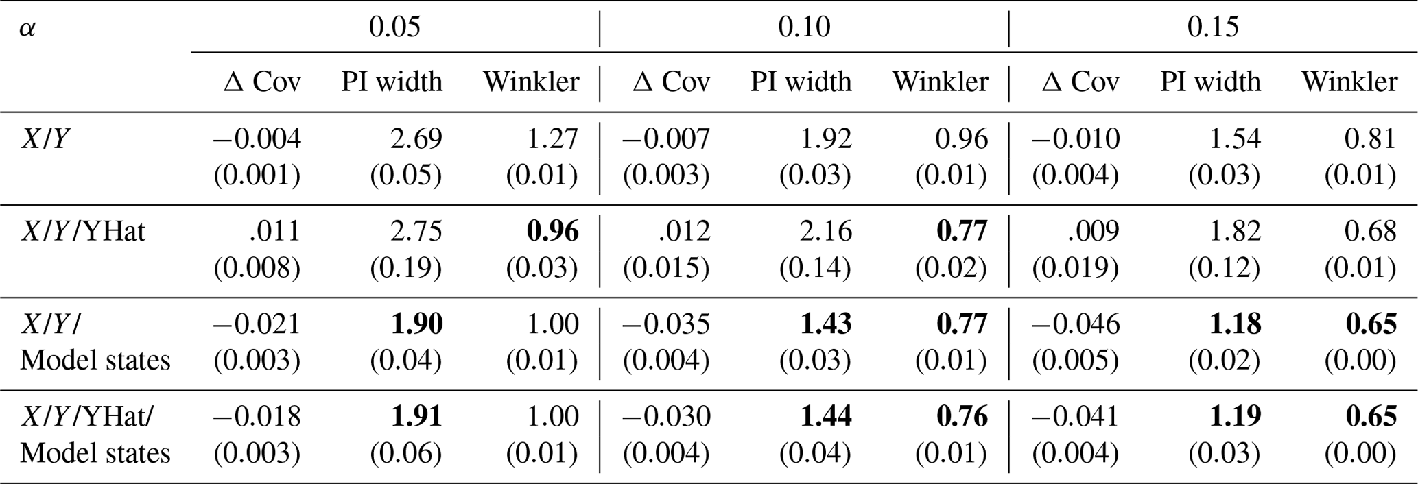
Table F2 shows the results when the lagged target variable is included in the feature set, as done in the original work Auer et al. (2023). Note that this is typically not feasible in streamflow prediction. However, to show how this affects the performance, we also evaluated these input combinations as such inclusion is possible in the lab setting.
Table F1HopCPT performance of the evaluated input combinations for the mis-coverage levels . The values represent the average over all basins. Bold numbers correspond to the best result for the respective metric in the experiment (PI width and Winkler score); significance is tested with a Mann–Whitney U test at p<0.005. The values in parentheses represent the standard deviation over the different seeds.
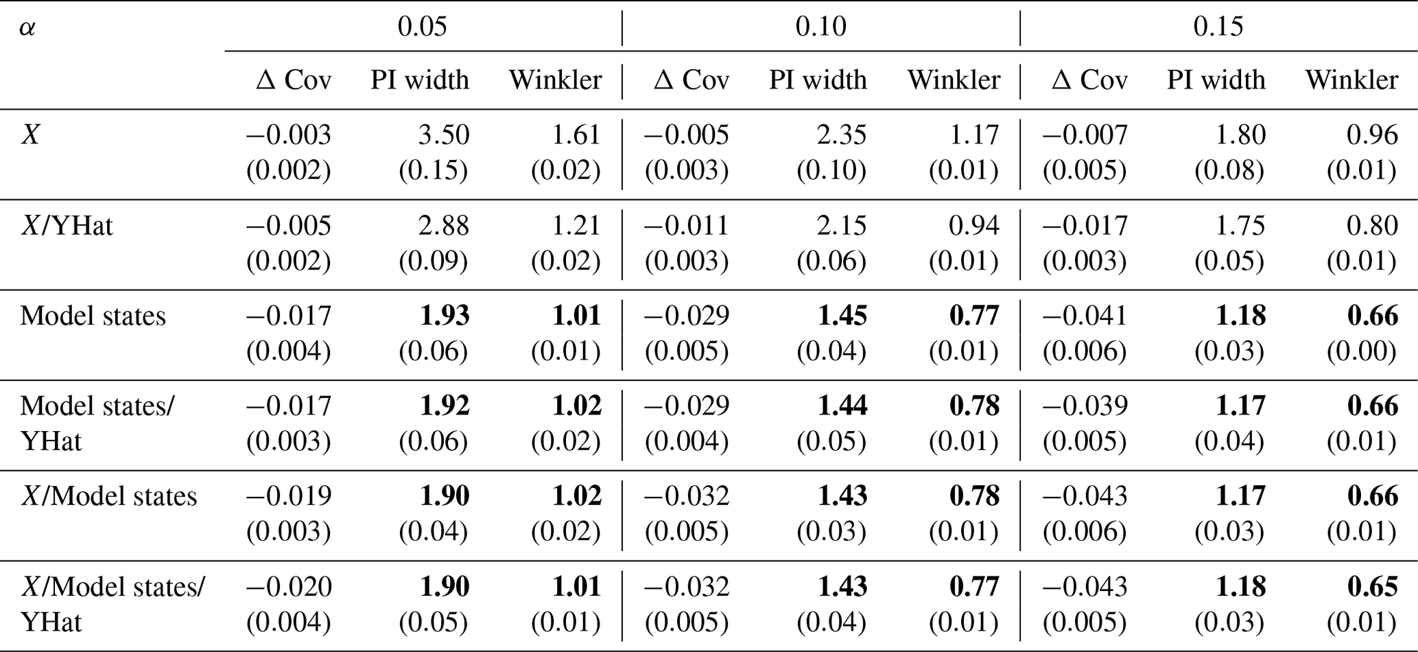
Table F2HopCPT performance with the input combinations which include the lagged target y for the mis-coverage levels . The values represent the average over all basins. Bold numbers correspond to the best result for the respective metric in the experiment (PI width and Winkler score). The values in parentheses represent the standard deviation over the different seeds.
Each non-deterministic experiment, apart from experiments with HopCPT-G, are repeated with 12 different seeds. HopCPT-G experiments are repeated with eight different seeds as the global models are computationally more demanding. For the latter experiments, we remove outlier runs where the training does not converge.
We conducted a hyperparameter grid search for each model. In the case of HopCPT, we did this individually for each input feature set. Each hyperparameter search was repeated with three seeds – the best average validation score was used as the selection criterion. The validation score for the LSTM and CMAL is the Nash–Sutcliffe efficiency (NSE) metric; for HopCPT, Bluecat, and kNN, we followed (Auer et al., 2023) and used the smallest PI width at an epoch with Δ Cov ≤0. To limit the number of grid search combinations for the LSTM and CMAL models, we split the hyperparameter into two sets which were tuned sequentially. The second set was trained given the result from the first set. Table H1 shows the parameters used in the hyperparameter search for the LSTM, CMAL, HopCPT, and HopCPT-G models. For Bluecat, we evaluated for . For kNN, we varied the share ks of samples, which defines the k parameter (i.e., ) and evaluated for .
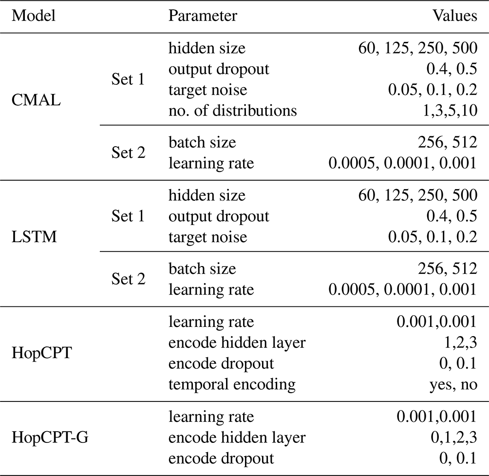
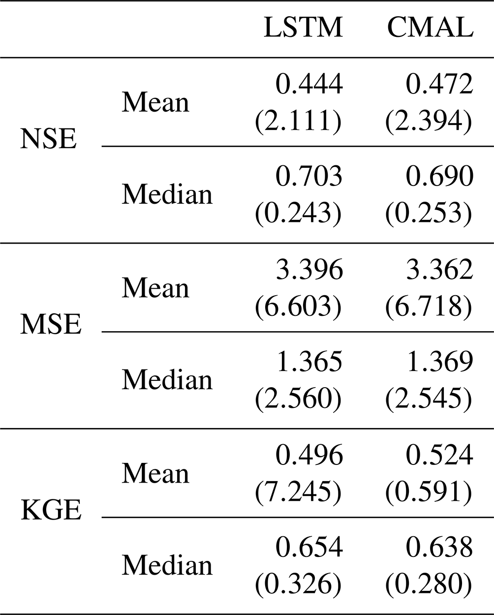
Table I1 shows the point prediction performance of LSTM and CMAL for Experiment II-b. The performance for the PUB prediction setting (Experiment II-b) is presented in Table I2. As in Klotz et al. (2022), CMAL outperforms the LSTM slightly. This could imply an advantage for the interval prediction. However, this is justifiable considering CMAL's greater volume of training data due to the fact that it does not need any calibration data.
Table I1Point prediction metrics for Experiment I and Experiment II-a. NSE: Nash–Sutcliffe efficiency (−∞,1] – high values are better. MSE: mean squared error – low values are better. KGE: Kling–Gupta efficiency (−∞,1] – high values are better. The variability of the metrics over the different basins and seeds is provided in the form of the standard deviation for the mean aggregation and in the form of the interquartile range (IQR) for the median aggregation.
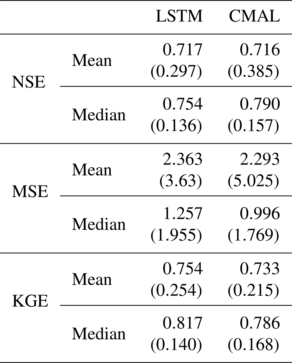
Table I2Point prediction metrics Experiment I and Experiment II-a (PUB). The values represent the average over all test basins of all splits. NSE: Nash–Sutcliffe efficiency (−∞,1] – high values are better. MSE: mean squared error – low values are better. KGE: Kling–Gupta efficiency (−∞,1] – high values are better. The variability of the metrics over the different basins and seeds is provided in the form of the standard deviation for the mean aggregation and in the form of the interquartile range (IQR) for the median aggregation.
J1 Experiment I-b – additional shift examples
In Experiment I-b, we show an example where a shift in the data highlights the advantages of the online mode for HopCPT. Figure J1 and J2 show two additional examples, both from the same basin, for different months.
J2 Experiment II-b – PUB results per fold
Table J1 shows the results of the PUB experiment for the individual folds. The performance varies between the folds; however, the ranking of the different models is consistent over all folds.
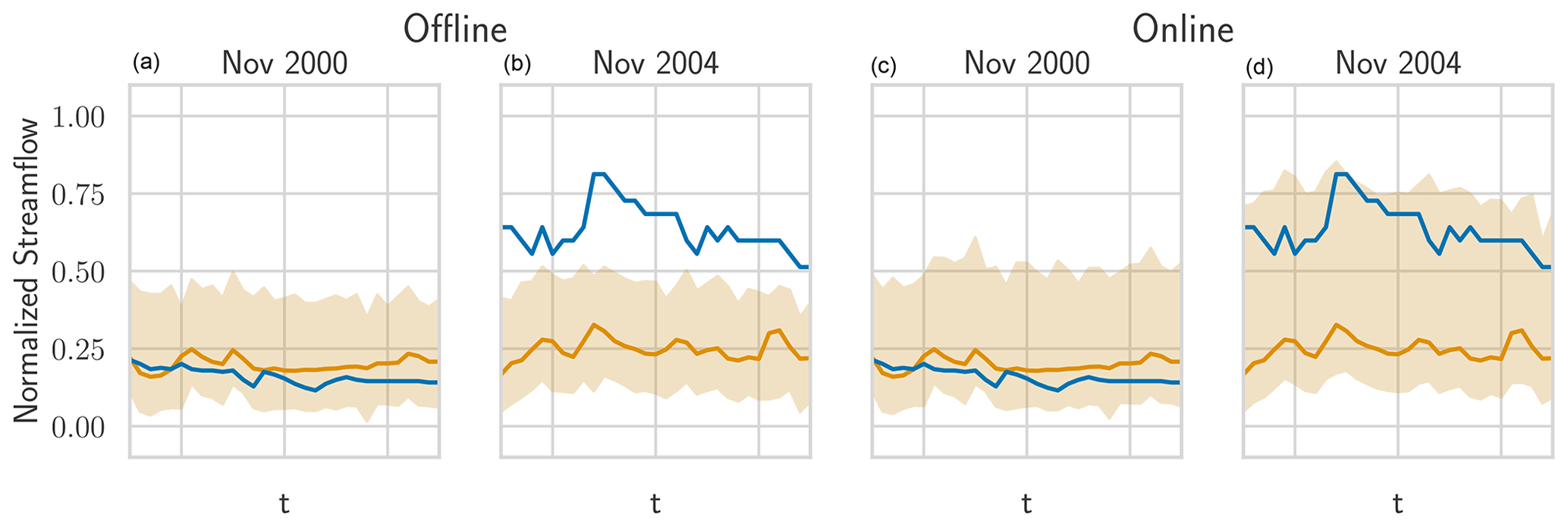
Figure J1The real streamflow (blue), the prediction (gold), and HopCPT's prediction interval (light gold) for a basin (ID no. 12447390) in November 2000 and October 2004. Panels (a) and (b) show HopCPT in offline mode; panels (c) and (d) show it in online mode. The online mode allows HopCPT to account for the distribution shift in November 2004.
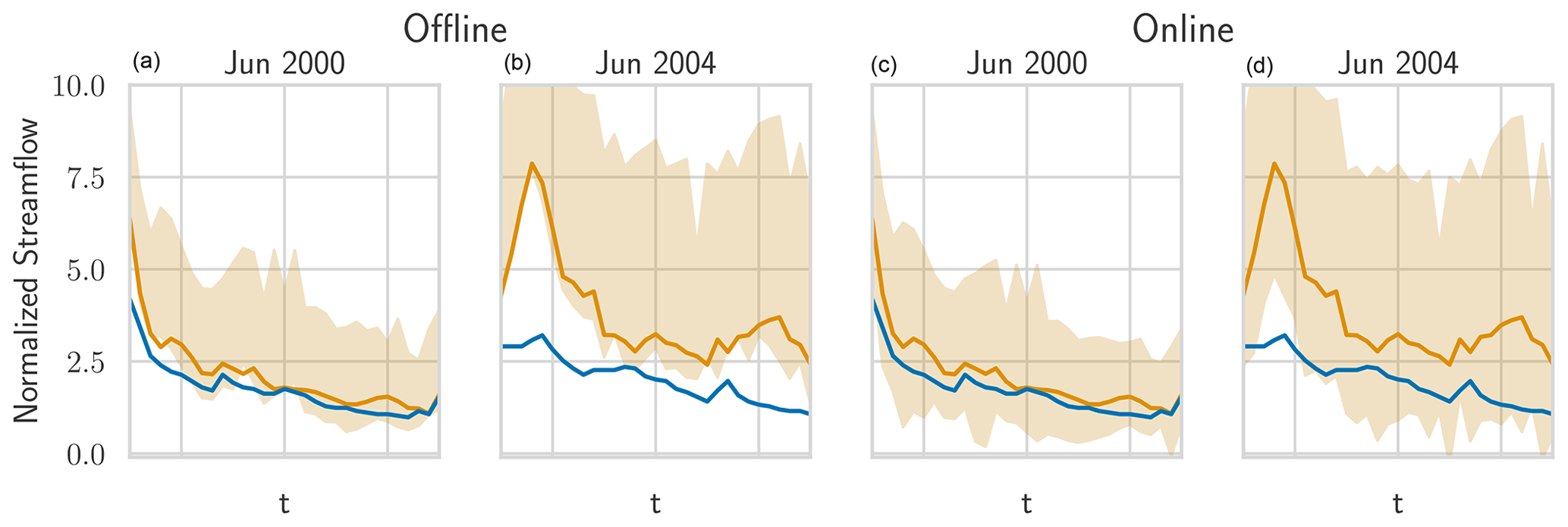
Figure J2The real streamflow (blue), the prediction (gold), and HopCPT's prediction interval (light gold) for a basin (ID no. 12447390) in June 2000 and October 2004. Panels (a) and (b) show HopCPT in offline mode; panels (c) and (d) show it in online mode. The online mode allows HopCPT to account for the distribution shift in June 2004.
Table J1PUB performance over the individual folds for the mis-coverage levels . The values represent the average over all test basins of the respective fold. Bold numbers correspond to the best result for the respective metric in the experiment (PI width and Winkler score). The values in parentheses represent the standard deviation over the different seeds.
J3 Experiment III – additional peak-flow evaluations
Figure J3 shows the peak-flow results for HopCPT with different memory update frequencies (see Experiment I-b). The coverage difference between different update frequencies does not notably change when only peak flows are considered. Figure J4 presents the peak-flow results for the PUB setting (see Experiment II-b). Similarly, as in the gauged-basin setting, the PUB training improves the coverage of HopCPT notably. CMAL coverage is rather constant over the different peak-flow shares.
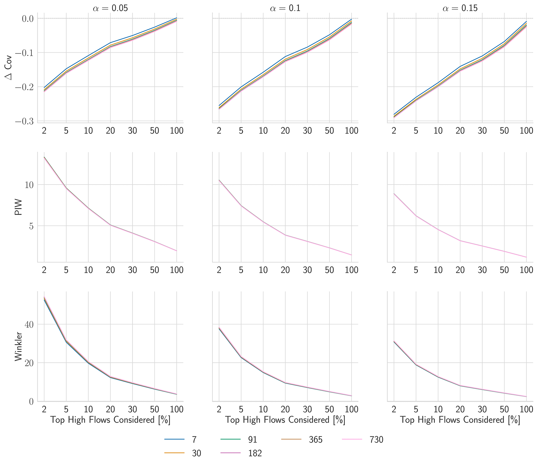
Figure J3Evaluation metrics for high flows with a varying share of considered time steps. The different runs represent different update frequencies (setting of Experiment I-b).
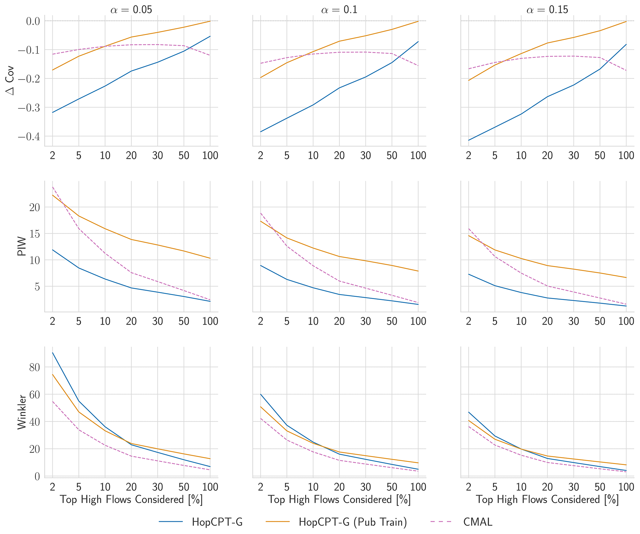
Figure J4Evaluation metrics for high flows with varying share of considered time steps in the ungauged-basin setting (setting of Experiment II-b).
The code repository is available at https://doi.org/10.5281/zenodo.10674231 (Auer, 2024a). The trained base model (LSTM) and the utilized model states, as well as the global HopCPT models, are available at https://doi.org/10.5281/zenodo.10653863 (Auer, 2024b). The trained CMAL models for the non-PUB experiments are available at https://doi.org/10.5281/zenodo.10654345 (Auer, 2024c), and the CMAL models for the PUB experiments are available at https://doi.org/10.5281/zenodo.10654399 (Auer, 2024d). The data for CAMELS can be accessed for free on the NCAR's official website (https://gdex.ucar.edu/dataset/camels/file.html, Addor et al., 2017b). The expanded Maurer forcings, which include data on daily minimum and maximum temperatures, are available for download at https://doi.org/10.4211/hs.17c896843cf940339c3c3496d0c1c077 (Kratzert, 2019).
AA, DK, and MG designed all the experiments. GN and FK checked the adequacy of the experiments and provided feedback. AA conducted all the experiments, and the results were analyzed by AA, DK, and MG. GN, DK, AA, and MG designed the structure of the exposition. All the authors contributed to the writing process, with AA, DK, and MG doing the majority of the writing. AA created all the figures. DK and SH supervised the article.
The contact author has declared that none of the authors has any competing interests.
Publisher’s note: Copernicus Publications remains neutral with regard to jurisdictional claims made in the text, published maps, institutional affiliations, or any other geographical representation in this paper. While Copernicus Publications makes every effort to include appropriate place names, the final responsibility lies with the authors.
We thank Carlo Albert for suggesting input perturbation analysis as future work. The ELLIS Unit Linz, the LIT AI Lab, and the Institute for Machine Learning are supported by the Federal State Upper Austria. We thank the projects Medical Cognitive Computing Center (MC3), INCONTROL-RL (project no. FFG-881064), PRIMAL (project no. FFG-873979), S3AI (project no. FFG-872172), DL for GranularFlow (project no. FFG-871302), EPILEPSIA (project no. FFG-892171), AIRI FG 9-N (project nos. FWF-36284 and FWF-36235), AI4GreenHeatingGrids (project no. FFG-899943), INTEGRATE (project no. FFG-892418), ELISE (H2020-ICT-2019-3 ID no. 951847), and Stars4Waters (HORIZON-CL6-2021-CLIMATE-01-01). We thank Audi.JKU Deep Learning Center, TGW Logistics Group GmbH, Silicon Austria Labs (SAL), FILL Gesellschaft mbH, Anyline GmbH, Google, ZF Friedrichshafen AG, Robert Bosch GmbH, UCB Biopharma SRL, Merck Healthcare KGaA, Verbund AG, GLS (University of Waterloo), Software Competence Center Hagenberg GmbH, Borealis AG, TÜV Austria, Frauscher Sensonic, TRUMPF, and the NVIDIA Corporation. We acknowledge EuroHPC Joint Undertaking for awarding us access to LUMI at CSC, Finland; we used as many instances of the pattern LUMI at CSC, Finland, as the number of systems awarded via EuroHPC.
This research has been supported by the Federal State of Upper Austria, the Österreichische Forschungsförderungsgesellschaft (grant nos. FFG-881064, FFG-873979, FFG-872172, FFG-871302, FFG-892171, FFG-899943, and FFG-892418), the Österreichischer Wissenschaftsfonds (grant nos. FWF-36284 and FWF-36235), the European Union Horizon Framework Programme (grant nos. 951847 and HORIZON-CL6-2021-CLIMATE-01-01), the Audi.JKU Deep Learning Center, TGW Logistics Group GmbH, Silicon Austria Labs (SAL), FILL Gesellschaft mbH, Anyline GmbH, Google, ZF Friedrichshafen AG, Robert Bosch GmbH, UCB Biopharma SRL, Merck Healthcare KGaA, Verbund AG, GLS (University of Waterloo), Software Competence Center Hagenberg GmbH, Borealis AG, TÜV Austria, Frauscher Sensonic, TRUMPF, and the NVIDIA Corporation.
This paper was edited by Pierre Gentine and reviewed by Carlo Albert and Matteo Giuliani.
Addor, N., Newman, A. J., Mizukami, N., and Clark, M. P.: The CAMELS data set: catchment attributes and meteorology for large-sample studies, Hydrol. Earth Syst. Sci., 21, 5293–5313, https://doi.org/10.5194/hess-21-5293-2017, 2017a. a
Addor, N., Newman, A., Mizukami, M., and Clark, M. P.: Catchment attributes for large-sample studies data repository: Boulder, CO, UCAR/NCAR [data set], https://gdex.ucar.edu/dataset/camels/file.html 2017b. a
Angelopoulos, A. N. and Bates, S.: A gentle introduction to conformal prediction and distribution-free uncertainty quantification, arXiv [preprint], https://doi.org/10.48550/arXiv.2107.07511, 2021. a
Auer, A.: Code – A data-centric perspective on the information needed for hydrological uncertainty predictions, Zenodo [code], https://doi.org/10.5281/zenodo.10674231, 2024a. a
Auer, A.: Models and Model States – A data-centric perspective on the information needed for hydrological uncertainty predictions, Zenodo [data set], https://doi.org/10.5281/zenodo.10653863, 2024b. a
Auer, A.: CMAL – Non PUB – A data-centric perspective on the information needed for hydrological uncertainty predictions, Zenodo [data set], https://doi.org/10.5281/zenodo.10654345, 2024c. a
Auer, A.: CMAL – PUB – A data-centric perspective on the information needed for hydrological uncertainty predictions, Zenodo [data set], https://doi.org/10.5281/zenodo.10654399, 2024d. a
Auer, A., Gauch, M., Klotz, D., and Hochreiter, S.: Conformal Prediction for Time Series with Modern Hopfield Networks, in: Thirty-seventh Conference on Neural Information Processing Systems, New Orleans, Louisiana, USA, 10–16 December 2023, https://openreview.net/forum?id=KTRwpWCMsC (last access: 31 August 2024), 2023. a, b, c, d, e, f, g, h, i, j, k, l, m
Bertola, M., Blöschl, G., Bohac, M., Borga, M., Castellarin, A., Chirico, G. B., Claps, P., Dallan, E., Danilovich, I., Ganora, D., Gorbachova, L., Ledvinka, O., Mavrova-Guirguinova, M., Montanari, A., Ovcharuk, V., Viglione, A., Volpi, E., Arheimer, B., Aronica, G.T., Bonacci, O., Čanjevac, I., Csik, A., Frolova, N., Gnandt, B., Gribovszki, Z., Gül, A., Günther, K., Guse, B., Hannaford, J., Harrigan, S., Kireeva, M., Kohnová, S., Komma, J., Kriauciuniene, J., Kronvang, B., Lawrence, D., Lüdtke, S., Mediero, L., Merz, B., Molnar, P., Murphy, C., Oskoruš, D., Osuch, M., Parajka, J., Pfister, L., Radevski, I., Sauquet, E., Schröter, K., Šraj, M., Szolgay, J., Turner, S., Valent, P., Veijalainen, N., Ward, P. J., Willems, P., and Zivkovic, N.: Megafloods in Europe can be anticipated from observations in hydrologically similar catchments, Nat. Geosci., 16, 982–988, https://doi.org/10.1038/s41561-023-01300-5, 2023. a, b, c
Beven, K.: Facets of uncertainty: epistemic uncertainty, non-stationarity, likelihood, hypothesis testing, and communication, Hydrolog. Sci. J., 61, 1652–1665, https://doi.org/10.1080/02626667.2015.1031761, 2016a. a
Beven, K.: Facets of uncertainty: epistemic uncertainty, non-stationarity, likelihood, hypothesis testing, and communication, Hydrolog. Sci. J., 61, 1652–1665, 2016b. a
Beven, K. and Binley, A.: GLUE: 20 years on, Hydrol. Process., 28, 5897–5918, 2014. a
Bhatnagar, A., Wang, H., Xiong, C., and Bai, Y.: Improved Online Conformal Prediction via Strongly Adaptive Online Learning, in: International Conference on Machine Learning, Honolulu, Hawaii, USA, 2023, https://api.semanticscholar.org/CorpusID:256868761 (last access: 31 August 2024), 2023. a
Bishop, C. M.: Mixture density networks, Tech. rep., Neural Computing Research Group, https://publications.aston.ac.uk/id/eprint/373/1/NCRG_94_004.pdf (last access: 5 September 2024), 1994. a
Clark, M. P., Wilby, R. L., Gutmann, E. D., Vano, J. A., Gangopadhyay, S., Wood, A. W., Fowler, H. J., Prudhomme, C., Arnold, J. R., and Brekke, L. D.: Characterizing uncertainty of the hydrologic impacts of climate change, Current Climate Change Reports, 2, 55–64, 2016. a
Demargne, J., Wu, L., Regonda, S. K., Brown, J. D., Lee, H., He, M., Seo, D.-J., Hartman, R., Herr, H. D., Fresch, M., Schaake, J., and Zhu, Y.: The science of NOAA's operational hydrologic ensemble forecast service, B. Am. Meteorol. Soc., 95, 79–98, 2014. a
Foygel Barber, R., Candes, E. J., Ramdas, A., and Tibshirani, R. J.: Conformal prediction beyond exchangeability, arXiv [preprint], https://doi.org/10.48550/arXiv.2202.13415, 2022. a, b
Frame, J. M., Kratzert, F., Klotz, D., Gauch, M., Shalev, G., Gilon, O., Qualls, L. M., Gupta, H. V., and Nearing, G. S.: Deep learning rainfall–runoff predictions of extreme events, Hydrology and Earth System Sciences, 26, 3377–3392, 2022. a
Gauch, M., Mai, J., and Lin, J.: The proper care and feeding of CAMELS: How limited training data affects streamflow prediction, Environ. Modell. Softw., 135, 104926, https://doi.org/10.1016/j.envsoft.2020.104926, 2021. a
Geirhos, R., Jacobsen, J.-H., Michaelis, C., Zemel, R. S., Brendel, W., Bethge, M., and Wichmann, F.: Shortcut learning in deep neural networks, Nature Machine Intelligence, 2, 665–673, https://api.semanticscholar.org/CorpusID:215786368 (last access: 31 August 2024), 2020. a
Gibbs, I. and Candes, E. J.: Adaptive conformal inference under distribution shift, Adv. Neur. In., 34, 1660–1672, 2021. a
Gupta, A. and Govindaraju, R. S.: Uncertainty quantification in watershed hydrology: Which method to use?, J. Hydrol., 616, 128749, https://doi.org/10.1016/j.jhydrol.2022.128749, 2023. a
Haines, A., Finlayson, B., and McMahon, T.: A Global Classification of River Regimes, Appl. Geogr., 8, 255–272, https://doi.org/10.1016/0143-6228(88)90035-5, 1988. a
Hamilton, J. D.: Analysis of time series subject to changes in regime, J. Econometrics, 45, 39–70, 1990. a, b
Harris, N. M., Gurnell, A. M., Hannah, D. M., and Petts, G. E.: Classification of river regimes: a context for hydroecology, Hydrol. Process., 14, 2831–2848, https://doi.org/10.1002/1099-1085(200011/12)14:16/17<2831::AID-HYP122>3.0.CO;2-O, 2000. a
Kavetski, D., Kuczera, G., and Franks, S. W.: Bayesian analysis of input uncertainty in hydrological modeling: 2. Application, Water Resour. Res., 42, W03407, https://doi.org/10.1029/2005WR004368, 2006. a
Klotz, D., Kratzert, F., Gauch, M., Keefe Sampson, A., Brandstetter, J., Klambauer, G., Hochreiter, S., and Nearing, G.: Uncertainty estimation with deep learning for rainfall–runoff modeling, Hydrol. Earth Syst. Sci., 26, 1673–1693, https://doi.org/10.5194/hess-26-1673-2022, 2022. a, b, c, d, e, f, g, h, i, j
Koutsoyiannis, D. and Montanari, A.: Bluecat: A Local Uncertainty Estimator for Deterministic Simulations and Predictions, Water Resour. Res., 58, e2021WR031215, https://doi.org/10.1029/2021WR031215, 2022. a, b, c
Kratzert, F.: CAMELS Extended Maurer Forcing Data, Hydroshare [data set], https://doi.org/10.4211/hs.17c896843cf940339c3c3496d0c1c077, 2019. a
Kratzert, F., Klotz, D., Herrnegger, M., Sampson, A. K., Hochreiter, S., and Nearing, G. S.: Toward Improved Predictions in Ungauged Basins: Exploiting the Power of Machine Learning, Water Resour. Res., 55, 11344–11354, https://doi.org/10.1029/2019WR026065, 2019a. a, b, c
Kratzert, F., Klotz, D., Shalev, G., Klambauer, G., Hochreiter, S., and Nearing, G.: Towards learning universal, regional, and local hydrological behaviors via machine learning applied to large-sample datasets, Hydrol. Earth Syst. Sci., 23, 5089–5110, https://doi.org/10.5194/hess-23-5089-2019, 2019b. a
Kratzert, F., Klotz, D., Hochreiter, S., and Nearing, G. S.: A note on leveraging synergy in multiple meteorological data sets with deep learning for rainfall–runoff modeling, Hydrol. Earth Syst. Sci., 25, 2685–2703, https://doi.org/10.5194/hess-25-2685-2021, 2021. a
Kratzert, F., Gauch, M., Klotz, D., and Nearing, G.: HESS Opinions: Never train an LSTM on a single basin, Hydrol. Earth Syst. Sci. Discuss. [preprint], https://doi.org/10.5194/hess-2023-275, in review, 2024. a
Krzysztofowicz, R.: The case for probabilistic forecasting in hydrology, J. Hydrol., 249, 2–9, 2001. a, b
Lapuschkin, S., Wäldchen, S., Binder, A., Montavon, G., Samek, W., and Müller, K.-R.: Unmasking Clever Hans predictors and assessing what machines really learn, Nat. Commun., 10, 1096, https://doi.org/10.1038/s41467-019-08987-4, 2019. a
Li, W., Duan, Q., Miao, C., Ye, A., Gong, W., and Di, Z.: A review on statistical postprocessing methods for hydrometeorological ensemble forecasting, Wiley Interdisciplinary Reviews: Water, 4, e1246, https://doi.org/10.1002/wat2.1246, 2017. a
Mai, J., Shen, H., Tolson, B. A., Gaborit, É., Arsenault, R., Craig, J. R., Fortin, V., Fry, L. M., Gauch, M., Klotz, D., Kratzert, F., O'Brien, N., Princz, D. G., Rasiya Koya, S., Roy, T., Seglenieks, F., Shrestha, N. K., Temgoua, A. G. T., Vionnet, V., and Waddell, J. W.: The Great Lakes Runoff Intercomparison Project Phase 4: the Great Lakes (GRIP-GL), Hydrol. Earth Syst. Sci., 26, 3537–3572, https://doi.org/10.5194/hess-26-3537-2022, 2022. a
Montanari, A. and Koutsoyiannis, D.: A blueprint for process-based modeling of uncertain hydrological systems, Water Resour. Res., 48, W09555, https://doi.org/10.1029/2011WR011412, 2012. a
Montero-Manso, P. and Hyndman, R. J.: Principles and algorithms for forecasting groups of time series: Locality and globality, Int. J. Forecast., 37, 1632–1653, 2021. a
Nearing, G., Cohen, D., Dube, V., Gauch, M., Gilon, O., Harrigan, S., Hassidim, A., Klotz, D., Kratzert, F., Metzger, A., Nevo, S., Pappenberger, F., Prudhomme, C., Shalev, G., Shenzis, S., Tekalign, T. Y., Weitzner, D., and Matias, Y.: Global prediction of extreme floods in ungauged watersheds, Nature, 627, 559–563, 2024. a
Nearing, G. S., Tian, Y., Gupta, H. V., Clark, M. P., Harrison, K. W., and Weijs, S. V.: A philosophical basis for hydrological uncertainty, Hydrolog. Sci. J., 61, 1666–1678, 2016. a
Newman, A. J., Clark, M. P., Sampson, K., Wood, A., Hay, L. E., Bock, A., Viger, R. J., Blodgett, D., Brekke, L., Arnold, J. R., Hopson, T., and Duan, Q.: Development of a large-sample watershed-scale hydrometeorological data set for the contiguous USA: data set characteristics and assessment of regional variability in hydrologic model performance, Hydrol. Earth Syst. Sci., 19, 209–223, https://doi.org/10.5194/hess-19-209-2015, 2015. a
Newman, A. J., Mizukami, N., Clark, M. P., Wood, A. W., Nijssen, B., and Nearing, G.: Benchmarking of a Physically Based Hydrologic Model, J. Hydrometeorol., 18, 2215–2225, https://doi.org/10.1175/JHM-D-16-0284.1, 2017. a
Quandt, R. E.: The estimation of the parameters of a linear regression system obeying two separate regimes, J. Am. Stat. Assoc., 53, 873–880, 1958. a, b
Ramsauer, H., Schäfl, B., Lehner, J., Seidl, P., Widrich, M., Gruber, L., Holzleitner, M., Pavlović, M., Sandve, G. K., Greiff, V., Kreil, D., Kopp, M., Klambauer, G., Brandstetter, J., and Hochreiter, S.: Hopfield networks is all you need, in: 9th International Conference on Learning Representations (ICLR), Vienna, Austria, 2021, https://openreview.net/pdf/4dfbed3a6ececb7282dfef90fd6c03812ae0da7b.pdf (last access: 31 August 2024), 2021. a, b, c
Rozos, E., Koutsoyiannis, D., and Montanari, A.: KNN vs. Bluecat – Machine Learning vs. Classical Statistics, Hydrology, 9, 101, https://doi.org/10.3390/hydrology9060101, 2022. a
Samaniego, L., Kumar, R., Thober, S., Rakovec, O., Zink, M., Wanders, N., Eisner, S., Müller Schmied, H., Sutanudjaja, E. H., Warrach-Sagi, K., and Attinger, S.: Toward seamless hydrologic predictions across spatial scales, Hydrol. Earth Syst. Sci., 21, 4323–4346, https://doi.org/10.5194/hess-21-4323-2017, 2017. a
Schweppe, R., Thober, S., Müller, S., Kelbling, M., Kumar, R., Attinger, S., and Samaniego, L.: MPR 1.0: a stand-alone multiscale parameter regionalization tool for improved parameter estimation of land surface models, Geosci. Model Dev., 15, 859–882, https://doi.org/10.5194/gmd-15-859-2022, 2022. a
Shrestha, D. L. and Solomatine, D. P.: Data-driven approaches for estimating uncertainty in rainfall-runoff modelling, International Journal of River Basin Management, 6, 109–122, 2008. a
Vaswani, A., Shazeer, N., Parmar, N., Uszkoreit, J., Jones, L., Gomez, A. N., Kaiser, L. u., and Polosukhin, I.: Attention is All you Need, in: Advances in Neural Information Processing Systems, edited by: Guyon, I., Luxburg, U. V., Bengio, S., Wallach, H., Fergus, R., Vishwanathan, S., and Garnett, R., vol. 30, Curran Associates, Inc., Long Beach, California, USA, 2017, https://proceedings.neurips.cc/paper_files/paper/2017/file/3f5ee243547dee91fbd053c1c4a845aa-Paper.pdf (last access: 31 August 2024), 2017. a, b
Vovk, V., Gammerman, A., and Shafer, G.: Algorithmic learning in a random world, Springer Science & Business Media, ISBN 978-0-387-00152-4, 2005. a, b, c
Wani, O., Beckers, J. V. L., Weerts, A. H., and Solomatine, D. P.: Residual uncertainty estimation using instance-based learning with applications to hydrologic forecasting, Hydrol. Earth Syst. Sci., 21, 4021–4036, https://doi.org/10.5194/hess-21-4021-2017, 2017. a, b
Xu, C. and Xie, Y.: Conformal prediction for time series, arXiv [preprint], https://doi.org/10.48550/arXiv.2010.09107, 2022a. a, b
Xu, C. and Xie, Y.: Sequential Predictive Conformal Inference for Time Series, arXiv [preprint], https://doi.org/10.48550/arXiv.2212.03463, 2022b. a
Zaffran, M., Dieuleveut, A., F'eron, O., Goude, Y., and Josse, J.: Adaptive Conformal Predictions for Time Series, in: International Conference on Machine Learning, Baltimore, Maryland, USA, 17–23 July 2022, https://api.semanticscholar.org/CorpusID:246863519 (last access: 31 August 2024), 2022. a
The calibration data are not part of the training data of the underlying prediction model, as is standard in CP. This property is very important because the prediction model can arbitrarily overfit the training data. If we were to estimate error bands or probabilities on top of that, we would get overconfident uncertainty estimates (i.e., very thin bars). Notably, this is not a specific limitation of conformal prediction or HopCPT as such since predictions based on the training data are, in general, distorted because of overfitting phenomena.
Note that we use the alternative proposal presented in Appendix E of the original work as it is computationally more efficient.
Here, we assume that the model state at time t already considers the input features of time step t.
and refer to the upper and lower bounds of the interval, respectively.
CMAL can be considered to be a global model
Only the calibration data are used.
- Abstract
- Introduction
- Methods
- Data and experiments
- Results and discussion
- Conclusions and outlook
- Appendix A: Overview
- Appendix B: Model intercomparison
- Appendix C: Bluecat
- Appendix D: HopCPT – training
- Appendix E: HopCPT, modern Hopfield networks, and transformer attention
- Appendix F: Input information
- Appendix G: Experiment details
- Appendix H: Hyperparameter search
- Appendix I: Point prediction metrics
- Appendix J: Extended results
- Code and data availability
- Author contributions
- Competing interests
- Disclaimer
- Acknowledgements
- Financial support
- Review statement
- References