the Creative Commons Attribution 4.0 License.
the Creative Commons Attribution 4.0 License.
 | 03 Sep 2024
Multi-decadal fluctuations in root zone storage capacity through vegetation adaptation to hydro-climatic variability have minor effects on the hydrological response in the Neckar River basin, Germany
Markus Hrachowitz
Gerrit Schoups
Climatic variability can considerably affect catchment-scale root zone storage capacity (Sumax), which is a critical factor regulating latent heat fluxes and thus the moisture exchange between land and atmosphere as well as the hydrological response and biogeochemical processes in terrestrial hydrological systems. However, direct quantification of changes in Sumax over long time periods and the mechanistic drivers thereof at the catchment scale are missing so far. As a consequence, it remains unclear how climatic variability, such as precipitation regime or canopy water demand, affects Sumax and how fluctuations in Sumax may influence the partitioning of water fluxes and therefore also affect the hydrological response at the catchment scale. Based on long-term daily hydrological records (1953–2022) in the upper Neckar River basin in Germany, we found that variability in hydro-climatic conditions, with an aridity index IA (i.e. ) ranging between ∼ 0.9 and 1.1 over multiple consecutive 20-year periods, was accompanied by deviations ΔIE between −0.02 and 0.01 from the expected IE inferred from the long-term parametric Budyko curve. Similarly, fluctuations in Sumax, ranging between ∼ 95 and 115 mm or ∼ 20 %, were observed over the same time period. While uncorrelated with long-term mean precipitation and potential evaporation, it was shown that the magnitude of Sumax is controlled by the ratio of winter precipitation to summer precipitation (p < 0.05). In other words, Sumax in the study region does not depend on the overall wetness condition as for example expressed by IA, but rather on how water supply by precipitation is distributed over the year. However, fluctuations in Sumax were found to be uncorrelated with observed changes in ΔIE. Consequently, replacing a long-term average, time-invariant estimate of Sumax with a time-variable, dynamically changing formulation of that parameter in a hydrological model did not result in an improved representation of the long-term partitioning of water fluxes, as expressed by IE (and fluctuations ΔIE thereof), or in an improved representation of the shorter-term response dynamics.
Overall, this study provides quantitative mechanistic evidence that Sumax changes significantly over multiple decades, reflecting vegetation adaptation to climatic variability. However, this temporal evolution of Sumax cannot explain long-term fluctuations in the partitioning of water (and thus latent heat) fluxes as expressed by deviations ΔIE from the parametric Budyko curve over multiple time periods with different climatic conditions. Similarly, it does not have any significant effects on shorter-term hydrological response characteristics of the upper Neckar catchment. This further suggests that accounting for the temporal evolution of Sumax with a time-variable formulation of that parameter in a hydrological model does not improve its ability to reproduce the hydrological response and may therefore be of minor importance for predicting the effects of a changing climate on the hydrological response in the study region over the next decades to come.
- Article
(9254 KB) - Full-text XML
-
Supplement
(759 KB) - BibTeX
- EndNote


Vegetation is a key component of the terrestrial hydrological cycle as it shapes the hydrological functioning of catchments by regulating the long-term average partitioning of water into drainage and evaporative fluxes (i.e. latent heat), frequently expressed as the runoff ratio Cr = [–] and evaporative index IE = = [–], respectively. More specifically, vegetation transpiration, which despite uncertainties (Coenders-Gerrits et al., 2014) globally constitutes the largest fraction of all evaporative fluxes (Jasechko, 2018), is systematically controlled by the interplay between canopy water demand and water supply from the sub-surface (Donohue et al., 2007; Yang et al., 2016; Jaramillo et al., 2018; Mianabadi et al., 2019). To survive, vegetation needs continuous access to water stored in the sub-surface and access to roots to satisfy its canopy water demand. As a consequence, the vegetation present at any moment, and in particular its active root system, reflects its successful adaptation to the prevalent climatic conditions in a region (Laio et al., 2001; Schenk and Jackson, 2002; Rodriguez-Iturbe et al., 2007; Donohue et al., 2007; Gentine et al., 2012; Liancourt et al., 2012). Irrespective of the geometry, distribution, or structure of root systems, the maximum vegetation-accessible water storage volume in the unsaturated root zone of the sub-surface, hereafter referred to as the root zone storage capacity Sumax (mm), represents the hydrologically relevant information of root systems (Rodriguez-Iturbe et al., 2007; Nijzink et al., 2016a; Savenije and Hrachowitz, 2017; Gao et al., 2024). Therefore, Sumax directly reflects the hydrologically relevant information of root systems at the catchment scales. In response to a changing environment, these root systems of vegetation continuously adapt to allow the most efficient use of available energy and resources for survival. The driving factors of changes in root systems are thus also the driving factors of changes in Sumax, as Sumax inherently represents adaptations of the root system.
As a central part of hydrological systems, Sumax is also a critical parameter in hydrological and land surface models. As such, it can, in principle, be estimated as a function of root depth and the sub-surface pore volume between field capacity and permanent wilting point (Scrivner and Ruppert, 1970; Sivandran and Bras, 2012, 2013). However, these data are typically not available at sufficient levels of detail. Alternatively, catchment-scale Sumax can be estimated by three broad approaches. Firstly, it can be obtained by calibration as a parameter of a hydrological model (Nijzink et al., 2018; Bouaziz et al., 2020; Wang et al., 2023; Sriwongsitanon et al., 2023; Roberts et al., 2021; Bahremand and Hosseinalizadeh, 2022; Sadayappan et al., 2023; Tong et al., 2022). Secondly, based on optimality principles, there are some variables like transpiration, nitrogen uptake, or carbon gain that can be maximized to quantify Sumax (Guswa, 2008; McMurtrie et al., 2012; Sivandran and Bras, 2012; Yang et al., 2016; Speich et al., 2018). Thirdly, Sumax can be robustly estimated at the catchment scale directly from annual water deficits based on observed hydro-climatic data, i.e. precipitation and transpiration (e.g. Donohue et al., 2012; Gentine et al., 2012; Gao et al., 2014b; de Boer-Euser et al., 2016; Nijzink et al., 2016a; Dralle et al., 2021; McCormick et al., 2021; Hrachowitz et al., 2021; Stocker et al., 2023; van Oorschot et al., 2021, 2024). For applications of hydrological and land surface models, Sumax (or equivalent parameters) has, except for very few exceptions (Wagener et al., 2003; Merz et al., 2011; Bouaziz et al., 2022; Tempel et al., 2024), been assumed constant over time. As a major knowledge gap, it still remains unknown whether Sumax follows climatic variability and evolves over time, thereby reflecting vegetation adaptation to changing conditions.
In contrast, it is well understood that, due to the importance of vegetation for the hydrological functioning of terrestrial systems, anthropogenic land use management practices, such as deforestation and afforestation (Brown et al., 2005; Brath et al., 2006; Fenicia et al., 2009; Alila et al., 2009; Jaramillo et al., 2018; Teuling et al., 2019; Stephens et al., 2021; Hoek van Dijke et al., 2022; Ellison et al., 2024) or irrigation (e.g. AghaKouchak et al., 2015; Van Loon et al., 2016; Roodari et al., 2021), can induce major shifts in the partitioning between the major components of the terrestrial water and energy cycles and thus between IE and Cr. Two detailed recent studies with well-documented information on deforestation in several experimental catchments could establish explicit mechanistic links between the reduction in Sumax by > 50 % following deforestation and decreases in IE (and thus increases in Cr) from ∼ 0.4–0.5 to ∼ 0.1–0.3, depending on the catchment and the scale of deforestation (Nijzink et al., 2016a; Hrachowitz et al., 2021).
Mapping the shifts to lower IE that followed these land conversions from forest to grassland- and rangeland-type vegetation as a function of the aridity index IA = in the Budyko framework (Schreiber, 1904; Ol'Dekop, 1911; Budyko, 1974) corresponds well to the results of previous studies that suggest that, across the world, catchments dominated by grass exhibit a consistently lower IE at the same IA than forest environments (e.g. Zhang et al., 2001, 2004; Oudin et al., 2008). These differences in the long-term average IE are accounted for by parametric reformulations of the Budyko framework, such as the Tixeront–Fu equation (Tixeront, 1964; Fu, 1981). The lumped parameters (here: ω) of these expressions define long-term average catchment-specific positions in the IA–IE space. As such, the parameters are typically interpreted as encapsulating vegetation characteristics and all other hydro-climatic and physiographic properties of individual catchments besides IA (e.g. Roderick and Farquhar, 2011; Berghuijs and Woods, 2016). A frequent assumption is that, with changes in climatic conditions, represented here by IA, individual catchments can be expected to move to the associated new positions IE, following their specific trajectories defined by ω (e.g. Zhou et al., 2015; Bouaziz et al., 2022). However, several studies have demonstrated that catchments in many regions worldwide experience deviations ΔIE from their expected new IE following a change in IA (e.g. Jaramillo and Destouni, 2014; van der Velde et al., 2014; Jaramillo et al., 2018; Reaver et al., 2022; Ibrahim et al., 2024; Tempel et al., 2024).
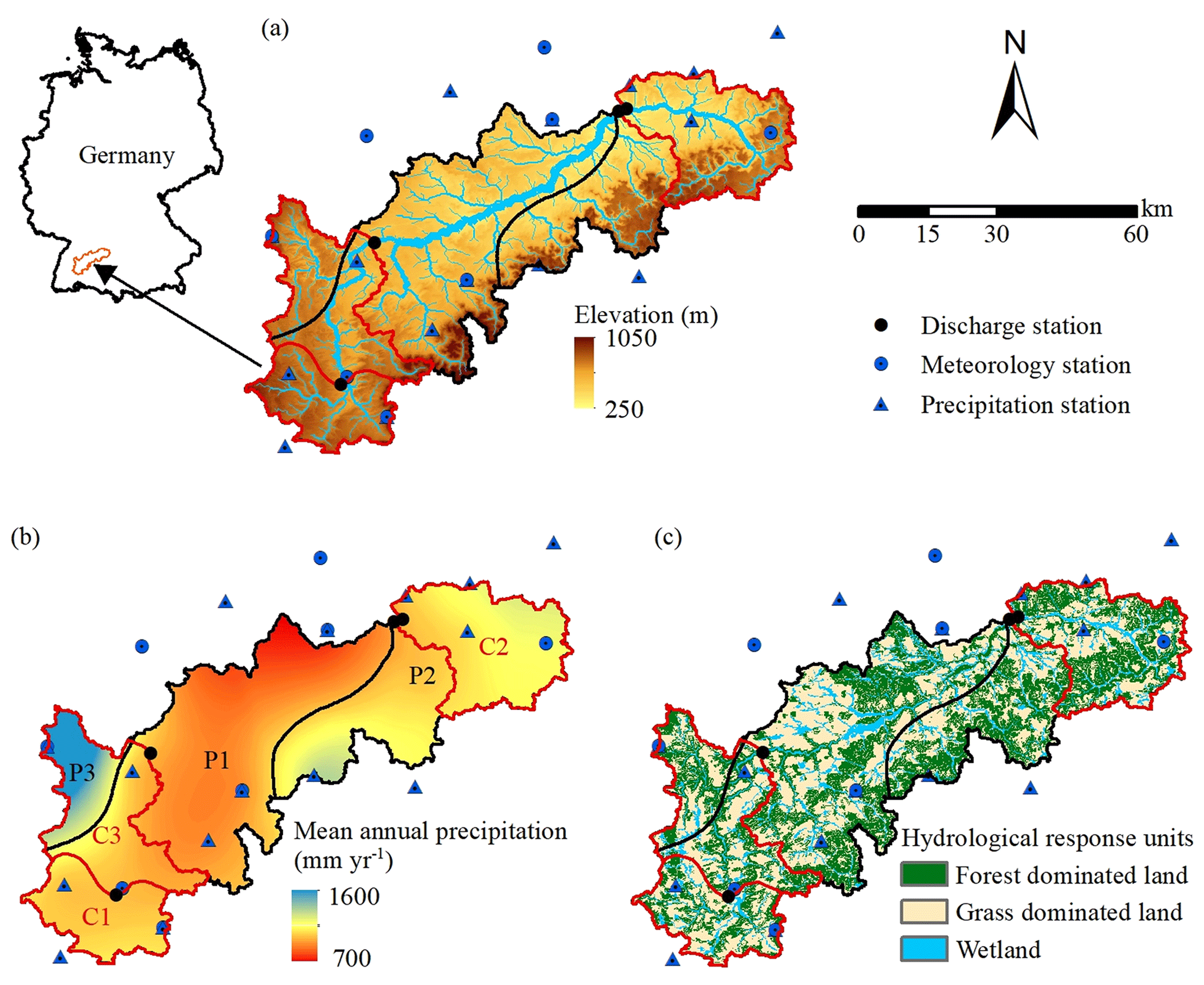
Figure 1(a) Elevation of the Neckar catchment with discharge and hydro-meteorological stations as well as the water sampling locations used in this study. (b) The spatial distribution of long-term mean annual precipitation in the upper Neckar catchment and the stratification into three distinct precipitation zones P1–P3 (black outline), together with the red outlines indicating three sub-catchments (C1: Rottweil; C2: Plochingen at the Fils River; C3: Horb) within the upper Neckar River basin. (c) Hydrological response units classified according to their land cover and topographic characteristics.
From the above, the following questions arise. (1) Following the notion that vegetation, i.e. individual plants but also the species composition of plant communities, continuously adapts to climatic conditions, does the catchment-scale root zone storage capacity Sumax change over multi-decadal timescales? (2) Do multi-decadal changes in the vegetation response, expressed by changes in Sumax, explain deviations ΔIE from the expected IE? (3) Does a time-variable representation of Sumax as a parameter in a hydrological model improve the models' ability to reproduce the hydrological response?
Building on previous studies, the objectives of this study in the upper Neckar River basin in Germany are therefore to provide an analysis of multi-decadal changes in Sumax as a result of changing climatic conditions over a 70-year period (1953–2022) and how this further affects hydrological dynamics. More specifically, we test the hypotheses that (1) Sumax changes significantly over multiple decades (reflecting vegetation adaptation to climatic variability), (2) changes in Sumax affect the long-term partitioning of drainage and evaporation and thus control deviations ΔIE from the catchment-specific trajectory in the Budyko space, and (3) a time-dynamic implementation of Sumax improves the representation of streamflow in a hydrological model.
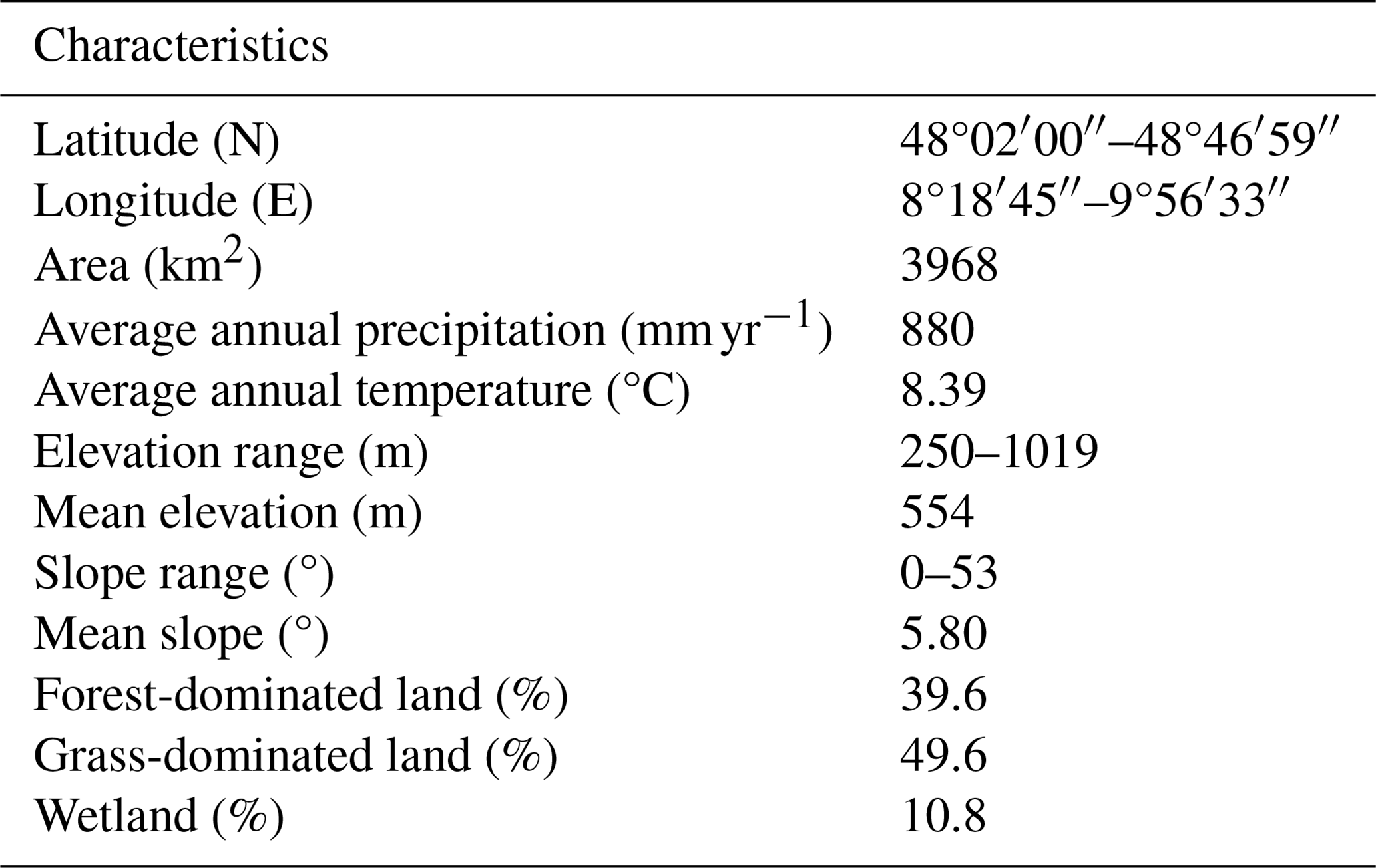
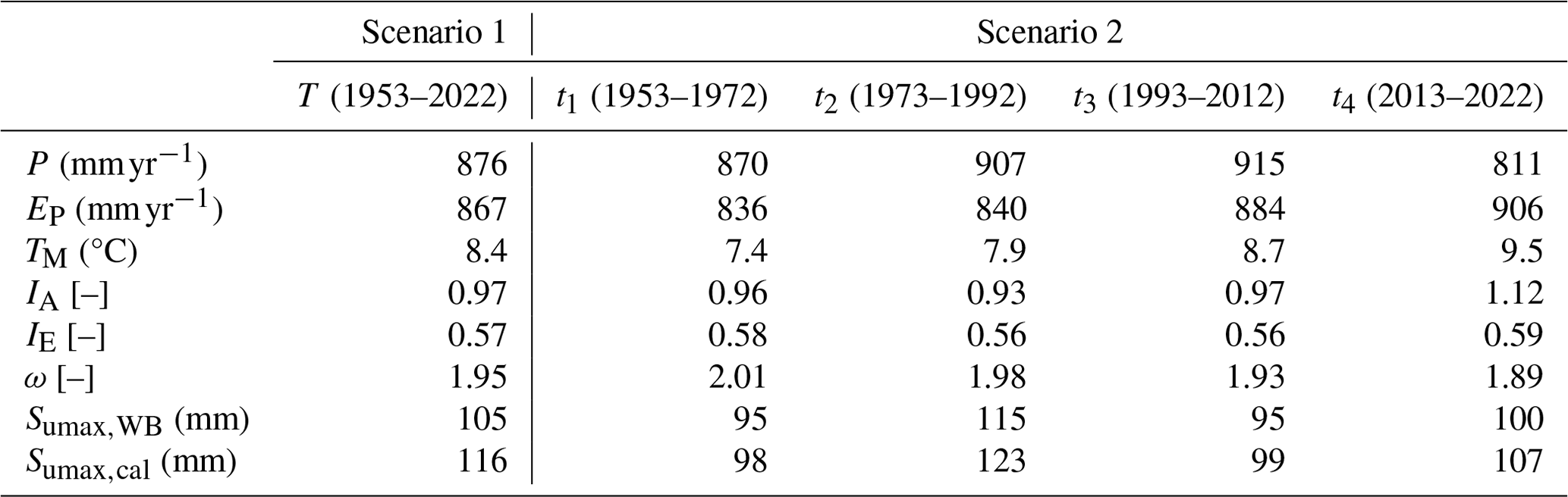
Table 2Mean annual precipitation P, potential evaporation EP, temperature TM, aridity index IA, evaporative index IE, parameter ω for the parametric Budyko framework, root zone storage capacity Sumax,WB, and Sumax,cal based on water balance data and hydrological model calibration for Scenario 1 (entire time period T: 1953–2022) and Scenario 2 (four sub-periods t1: 1953–1972, t2: 1973–1992, t3: 1993–2012, and t4: 2013–2022).
The upper Neckar River basin in south-western Germany covers an area of ∼ 4000 km2, with the Black Forest on the western side and the Swabian Jura on the south-eastern side. The river basin has a varying topography, with its elevation ranging from 250 m at the outlet in the north to about 1019 m in the south (Fig. 1a, Table 1). Following the elevation gradient, the landscape is dominated by terrace-like elements and undulating hills (∼ 50 %) with wide valleys used as grasslands and croplands in the lower regions, in particular in the south-eastern parts of the upper Neckar River basin, and by increasingly steep and narrow forested valleys (∼ 40 %) towards the southern parts and the remaining area that includes flat grassland in valley bottoms (∼ 10 %) (Fig. 1c). Annual mean precipitation (P) over the whole river basin has a considerable spatial heterogeneity ranging from ∼ 700 mm yr−1 in the lower parts of the basin to ∼ 1600 mm yr−1 over the Black Forest, with catchment-average long-term mean precipitation (P) reaching ∼ 880 mm yr−1 (Fig. 1b, Table 2). The catchment is characterized by a temperate, humid climate with warm, wet summers and cold, drier winters. Precipitation exhibits some seasonality with ∼ 500 mm yr−1 for the summer months (from May to October) and ∼ 380 mm yr−1 for the winter months (from November to April), respectively (Fig. 3). Although snow is in general not a major component of precipitation in the study region, snowmelt can have a significant influence during individual storm events. The long-term mean temperature is about 8.2 °C and the potential evaporation (EP) is about ∼ 860 mm yr−1, with an aridity index IA = ∼ 0.97 (Table 2).
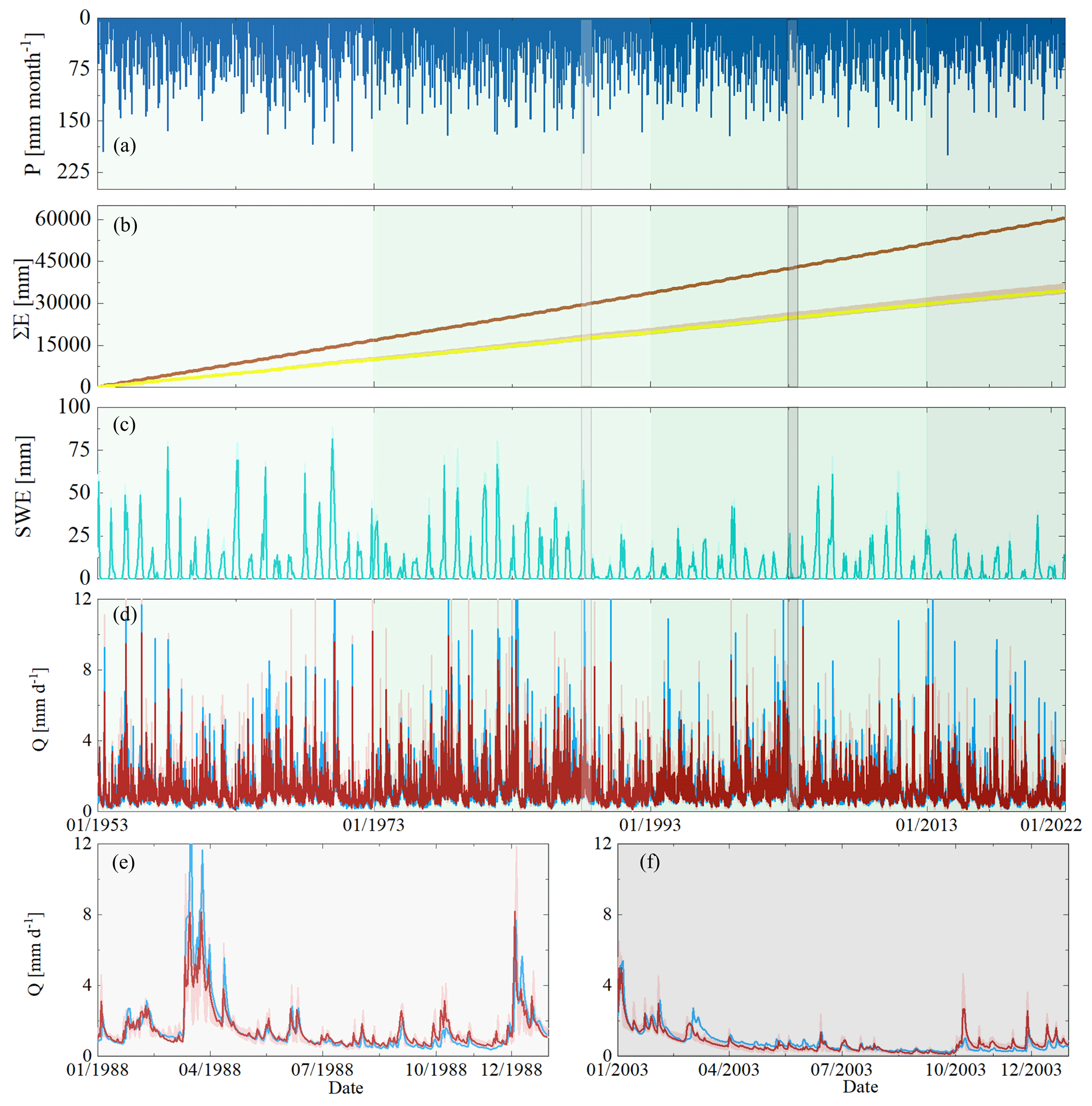
Figure 2(a) Time series of observed monthly precipitation P. (b) Daily cumulative evaporative fluxes for the entire time period (1953–2022), where the dark-brown line indicates the potential evaporation EP and the yellow lines and light-orange-shaded areas show the actual evaporation EA modelled using the best-fit parameter sets and the associated 5th and 95th percentiles of all feasible solutions calibrated based on the entire time period. (c) Monthly maximum values of the snow water equivalent (SWE) for the 1953–2022 time period, where the green line indicates the most balanced solution and the light-green shade indicates the 5th and 95th inter-quantile ranges obtained from all the Pareto optimal solutions calibrated based on the entire time period. (d) Observed (blue line) and modelled daily streamflow Q; the red line indicates the most balanced solution and the shaded area indicates the 5th and 95th percentiles of all feasible solutions calibrated based on the entire time period; and the different green background shades from lighter to darker indicate the sub-time periods from t1 to t4. Panels (e) and (f) zoom in to the observed and modelled streamflows for the selected wet year (light-grey shade, 1 January 1988–31 December 1988) and the dry year (grey shade, 1 January 2003–31 December 2003), respectively.
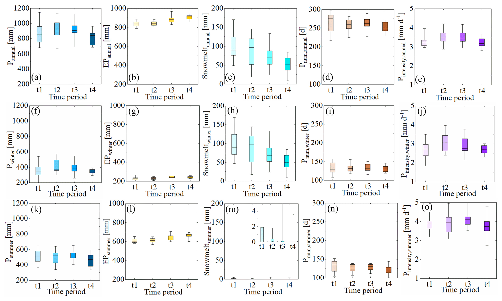
Figure 3The annual and seasonal variability (i.e. winter and summer) of selected climatic indices, including annual averages of precipitation (P), potential evaporation (EP), estimated snowmelt water, the number of precipitation days (Pnum), and the precipitation intensity (Pintensity) for the four sub-time periods (t1: 1953–1972, t2: 1973–1992, t3: 1993–2012, and t4: 2013–2022). (a–e) The annual variability of selected climatic indices. (f–j) The seasonal variability of selected climatic indices in the winter periods. (k–o) The seasonal variability of selected climatic indices in the summer periods.
3.1 Data
Daily hydro-meteorological data were available for the period 1 January 1953–31 December 2022 (Fig. 2). Daily precipitation and daily mean air temperature were obtained from stations operated by the German Weather Service (DWD). Precipitation was recorded at 15 stations and temperature measurements were available at 8 stations (Fig. 1) in or close to the study basin. Daily potential evaporation EP (mm d−1) was estimated using the Hargreaves equation based on the observed daily maximum and minimum temperatures, has been used in many previous studies, and has been shown to be a suitable method for modelling applications (Oudin et al., 2005). Daily mean discharge data for the period 1 January 1953–31 December 2022 at the outlet of the upper Neckar River basin at Plochingen station were provided by the German Federal Institute of Hydrology (BfG). In addition, data of daily mean discharge for the same time period from three sub-catchments within the upper Neckar River basin (Fig. 1) at the gauges Rottweil (C1; 422 km2), Plochingen at the Fils River (C2; 706 km2), and Horb (C3; 1111 km2) were available from the Environmental Agency of the Baden-Württemberg region (LUBW).
Based on the CORINE Land Cover data set of the upper Neckar River basin during the period 1 January 1953–31 December 2022 (https://land.copernicus.eu/en/products/global-dynamic-land-cover (last access: 27 August 2024), there is only very minor change (< 2 %) for all the defined land cover classes (Fig. 1c). The 90 m × 90 m digital elevation model of the study region (Fig. 1a) was obtained from the Hydrologic Derivatives for Modeling and Applications (HDMA) database of the United States Geological Survey (USGS) (Verdin, 2017; https://doi.org/10.5066/F7S180ZP) and used to derive the local topographic indices, including height above nearest drainage (HAND) and slope.
3.2 Data pre-processing
For the subsequent experiment (Sect. 4.2), the study basin was stratified into three zones P1–P3 that are characterized by a distinct long-term precipitation pattern (hereafter precipitation zones), following the approach described and implemented for the Neckar River basin by Wang et al. (2023). Briefly, Goovaerts (2000) and Lloyd (2005) showed that areal precipitation estimates informed by elevation data were often more accurate than those based on precipitation gauge observations alone (e.g. Hrachowitz and Weiler, 2011). Thus, to interpolate and estimate areal precipitation across the basin, we used co-kriging that considered elevation, as a preliminary analysis suggested lower errors. Finally, the individual precipitation estimates for each grid cell were used with k-means clustering to establish three clusters representing the three precipitation zones P1–P3 (see Fig. 1b).
To explore the fluctuations of Sumax over long timescales, we independently estimate the root zone storage capacity Sumax for four subsequent sub-periods of the available data record (t1–t4 in Table 2). To survive, root systems of vegetation and the associated vegetation-accessible water storage capacity Sumax respond to the ever-changing conditions of their environment. However, as these changes occur at the landscape scale and are mostly reflected in changes in the composition of plant species present in a specific spatial domain, fluctuations in Sumax largely occur at timescales that reflect the lifecycles of individual plants. Thus, periods of at least 20 years are required to reflect this and to allow for meaningful estimates of Sumax, as also demonstrated by many other studies (e.g. Gao et al., 2014b; Wang-Erlandsson et al., 2016; Singh et al., 2020; Stocker et al., 2023). We therefore had to strike a balance between the number of independent time periods (here: t1–t4) and the robustness of the associated Sumax estimates. We deliberately chose to emphasize fewer but longer time periods and thus rather reliable estimates of Sumax.
To test the hypotheses that the key vegetation parameter, i.e. the root zone storage capacity Sumax, evolves over multi-decadal timescales in response to changing hydro-climatic conditions and controls the deviations from expected trajectories in the Budyko space (thereby reflecting the need for time-variable implementations of Sumax as a parameter in a hydrological model), the following stepwise approach is designed. (1) Estimate the observed deviations ΔIE from the long-term average expected IE for four consecutive periods t1–t4 in the study period (Table 2). (2) Estimate the root zone storage capacity over the entire study period () and the four individual periods t1–t4 () based on observed water balance data. (3) Estimate the root zone storage capacity over the entire study period () and the four individual periods t1–t4 () by calibration of a hydrological model over the respective time periods to evaluate whether the changes in the calibrated Sumax,cal reflect changes in Sumax,WB directly estimated from water balance data from step (2). (4) Estimate the modelled deviations () from the expected IE using both a long-term average time-invariant and an individual for the four periods t1–t4 as model parameters.
4.1 Estimation of the temporal trajectory in the Budyko framework
Mapping aridity IA = , where EP is potential evaporation (mm d−1) and P is precipitation (mm d−1), against the evaporative index IE = = , where EA is actual evaporation (mm d−1) and Q is streamflow (mm d−1), the Budyko framework is an expression of the long-term average water balance for a catchment. It is based on the assumption of negligible storage change over the averaging time period, i.e. ∼ 0. As demonstrated by Han et al. (2020), this assumption holds for averaging periods ≥ 10 years for a large majority of catchments worldwide. Note that hereafter the term “evaporation” is used to refer to all combined evaporative fluxes, including interception and soil evaporation (Ei) as well as transpiration (ET), following the terminology proposed by Savenije (2004) and Miralles et al. (2020).
The analysis in this paper is based on the parametric Tixeront–Fu formulation of the Budyko framework (Tixeront, 1964; Fu, 1981):
where IE,T is the observed evaporative index over a chosen averaging period T, IA,T is the observed aridity index over the same period, and ωT is the associated catchment-specific parameter that represents all combined catchment properties other than IA.
In a theoretical catchment that only experiences changes in IA and no changes in any other hydro-climatic and/or physical catchment characteristics, it can be assumed that ωT remains constant over time, so that . This implies that, following a disturbance ΔIA in a subsequent time period ti+1, the catchment stays on its specific curve defined by ωT to a new . In such a case, ωT can thus be used to predict future hydrological partitioning IE. Based on this assumption, here we use the complete available hydro-climatic data record to estimate the long-term average ωOT as a reference over the entire 1953–2022 study period. The sub-division into the four time periods t1–t4 as shown in Table 2 is then allowed to estimate the expected in the individual periods t1–t4: depending on the shift in the observed aridity index along the x axis in ti ( = ), a catchment will move along its parametric Budyko curve defined by ωOT to a new expected position (Fig. 4).
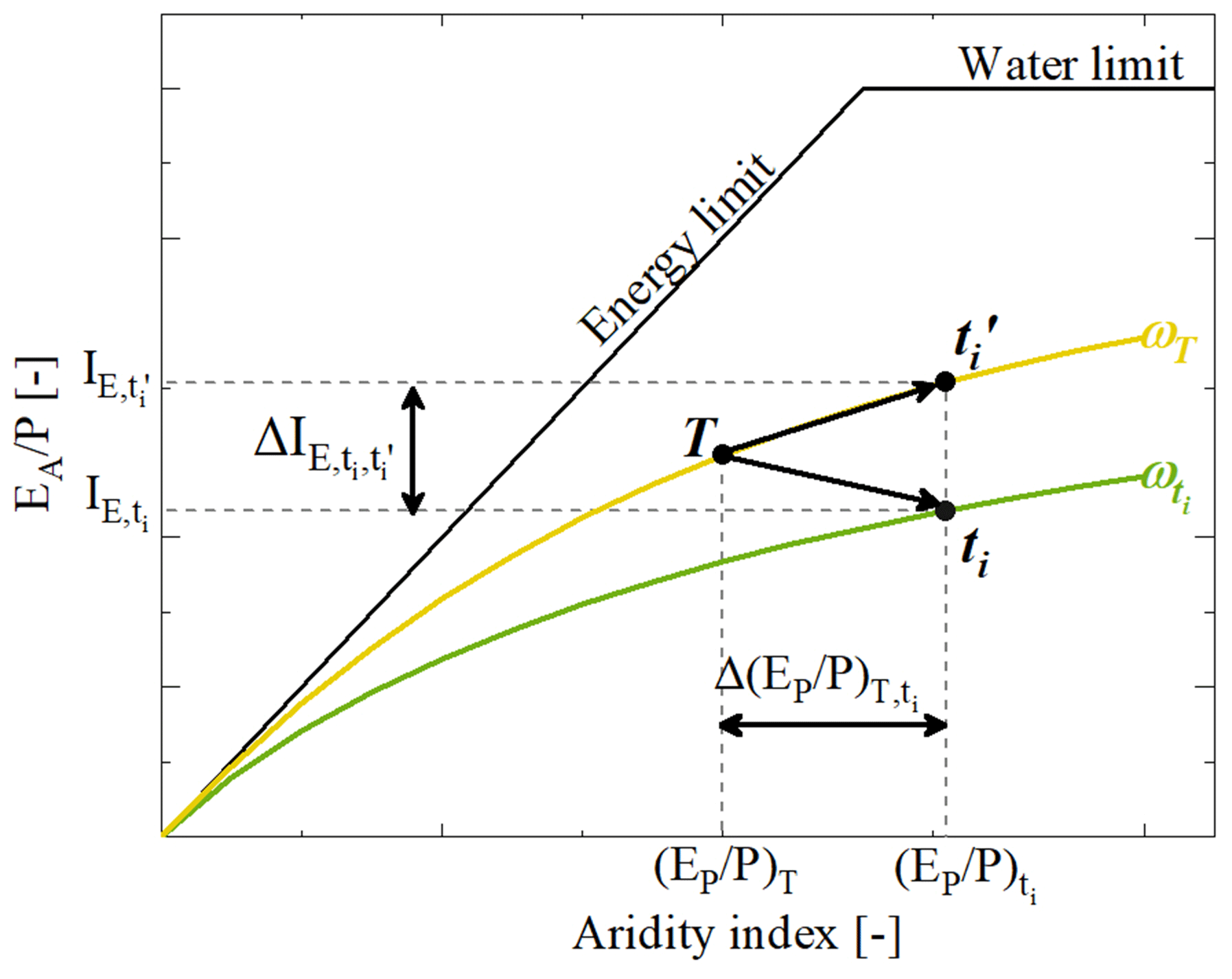
Figure 4Representation of the Budyko space, which shows the evaporative index (IE = ) as a function of the aridity index (IA = ) and the water and energy limits. A catchment with the long-term mean aridity index IA,T = and evaporative index IE,T = , which is derived from observed data of the entire time period, is plotted at location T on the parametric Budyko curve with ωT (yellow line) as the baseline. Based on the observed sub-time-period data with the aridity index = and evaporative index = , the same catchment is plotted at location ti on the parametric Budyko curve with (green line). A movement in the Budyko space towards along the ωT curve is shown as a result of a change in the aridity index with the assumption that the long-term mean Budyko curve trajectory and the parameter ω are transferable across time for an individual catchment, which results in a significant deviation between the observed evaporative index and the predicted evaporative index .
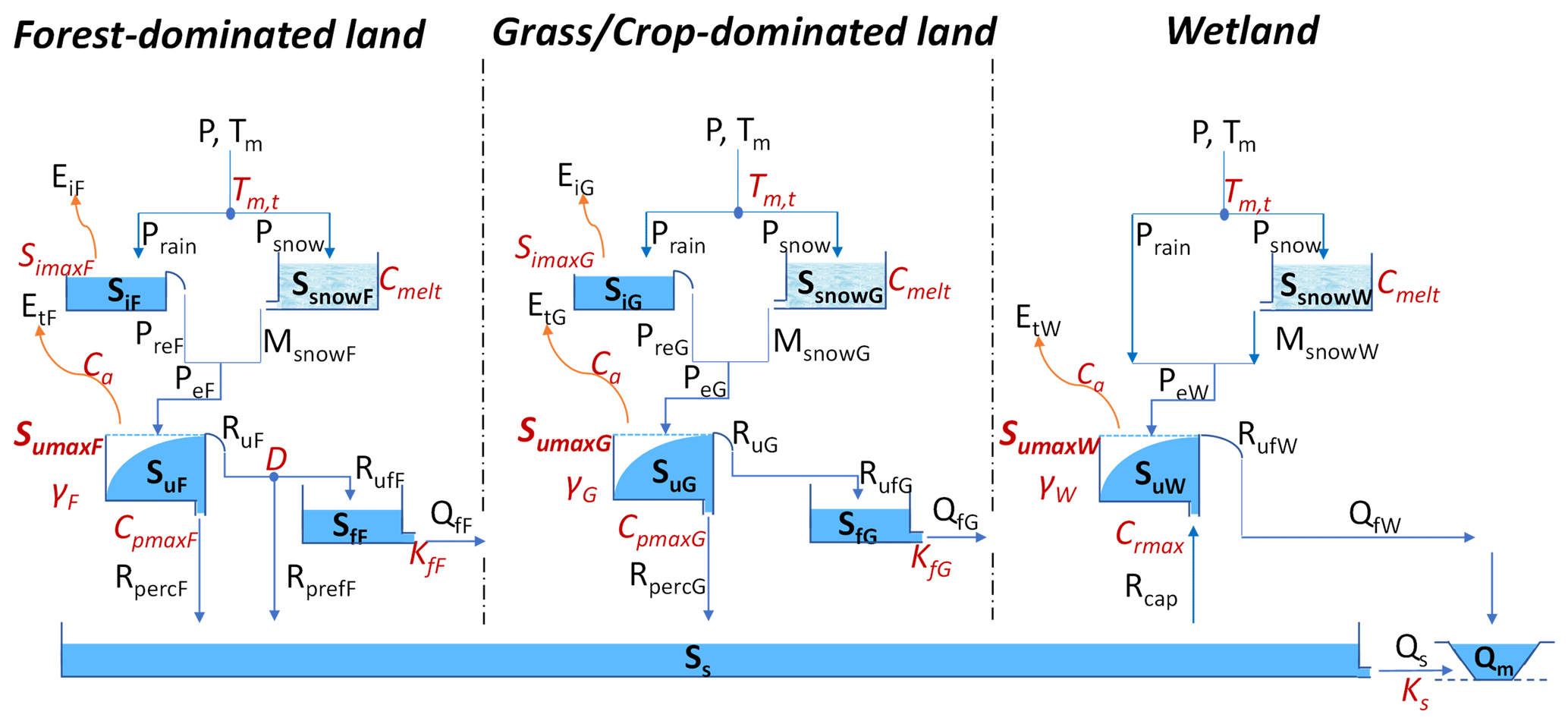
Figure 5Model structure of the distributed conceptual hydrological model, discretized into three parallel hydrological response units (HRUs), i.e. forest, grassland, and wetland in each precipitation zone from P1 to P3. The light-blue boxes indicate the hydrologically active individual storage volumes. The arrow lines indicate water fluxes and the model parameters are shown in red. All the symbols are described in Table S1 in the Supplement.
Based on the available data, we then estimate the individual observed together with the associated for each of the four time periods t1–t4 (Fig. 5). For each of the four time periods t1–t4, the deviation of from the catchment-specific expected , corresponding to a shift from ωT to , was then computed as = .
4.2 Estimation of the root zone storage capacity derived by the water balance method Sumax,WB
The root zone storage capacity is the maximum volume of water which can be held in soil pores of the unsaturated zone and which is accessible to root systems of vegetation for transpiration. Here the water balance method that is described in detail in previous papers (e.g. Gao et al., 2014b; Nijzink et al., 2016a; de Boer-Euser et al., 2016; Wang-Erlandsson et al., 2016; Bouaziz et al., 2020; Hrachowitz et al., 2021) is used to determine Sumax,WB. Briefly, Sumax,WB is estimated based on daily observations of precipitation (P), potential evaporation (EP), and streamflow (Q). As a first step, effective precipitation Pe (mm d−1) that enters the sub-surface is computed by accounting for interception evaporation by
where Ei (mm d−1) is the daily interception evaporation and Si (mm) is the interception storage. For each time step, Ei is determined by
Then, the effective precipitation Pe (mm d−1) is further estimated according to
where Simax (mm) is the maximum interception storage. As Sumax is not very sensitive to the choice of Simax, as previously shown by Hrachowitz et al. (2021) and Bouaziz et al. (2022), here we used a value of Simax = 2 mm, which was previously also used by de Boer-Euser et al. (2016).
Hereafter, the long-term mean transpiration (mm d−1) is estimated from the long-term water balance, with the assumption of no additional gains or losses:
where (mm d−1) is the long-term mean effective precipitation and (mm d−1) is the long-term mean observed streamflow. Considering the seasonal fluctuation of energy input, the daily transpiration Er (mm d−1) is estimated by subsequently scaling the daily potential evaporation EP (mm d−1) minus the interception evaporation Ei (mm d−1) (see Eqs. 2 and 3) by the long-term mean transpiration (mm d−1), according to (Bouaziz et al., 2022; Hrachowitz et al., 2021)
where (mm d−1) is the long-term mean potential evaporation and (mm d−1) is the long-term mean interception evaporation.
From daily storage deficits Srd,n(t) (mm) during dry periods, estimated as the cumulative sum of daily effective precipitation Pe (mm d−1) minus transpiration Er (mm d−1), the maximum storage deficit Srd,n of a specific year n is then computed as follows:
where t is the time step (d), t0,w is the day at the end of the wet period when the storage deficits are zero but Pe(t)−Er(t) < 0, and t0,d is the day when the storage deficits return to zero again after the beginning of the next wet period when the water supply exceeds the canopy water demand, i.e. (Pe(t)−Er(t)) > 0. Any cumulative precipitation surplus is assumed to be drained from the root zone and is released from the system either directly as streamflow or via recharge of the groundwater.
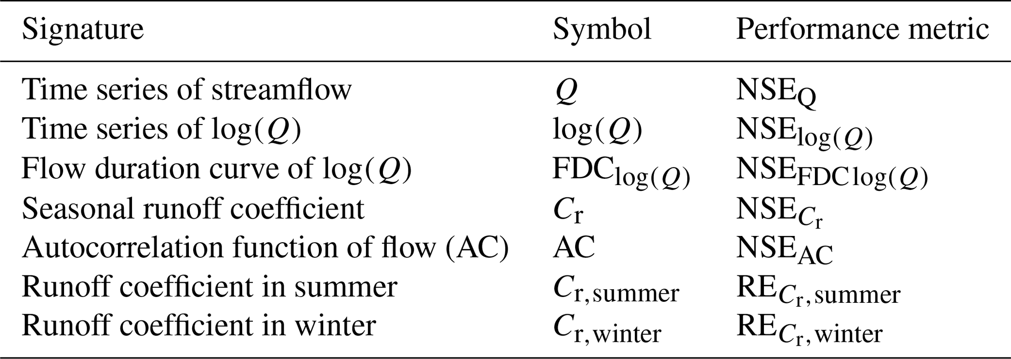
Table 3Flow signatures and the associated performance metrics used for model calibration and evaluation. The performance metrics include the Nash–Sutcliffe efficiency (NSE) and the relative error (RE).
The Gumbel extreme value distribution (Gumbel, 1941) was used previously by several other studies (Gao et al., 2014b; Nijzink et al., 2016a; de Boer-Euser et al., 2016; Bouaziz et al., 2020, 2022; Hrachowitz et al., 2021) to estimate the root zone storage capacity through the water balance approach. Based on fitting the Gumbel distribution to the maximum annual storage deficits for all n years during one of the four time periods t1–t4, the root zone storage capacity Sumax,WB can be derived from various return periods of the sequence of n maximum annual storage deficits Srd. Previous studies suggested that vegetation develops root zone storage capacities large enough to survive in dry spells with return periods of ∼ 20–40 years (Gao et al., 2014b; de Boer-Euser et al., 2016; Wang-Erlandsson et al., 2016; Hrachowitz et al., 2021). Therefore, here we define Sumax,WB as the maximum storage deficit in a 40-year period so that .
Using the above water-balance-based method, we determine Sumax,WB for the entire study period 1953–2022 () as well as individually for the four time periods t1–t4 () to quantify potential fluctuations of the root zone storage capacity reflecting the adaptation to changing climatic conditions.
4.3 Hydrological model
4.3.1 Model architecture
Loosely based on the flexible DYNAMITE modular modelling framework (e.g. Hrachowitz et al., 2014), here we used a semi-distributed, process-based model that was previously successfully implemented and tested for the Neckar study basin (Wang et al., 2023) and for many other contrasting environments worldwide (e.g. Prenner et al., 2018; Hulsman et al., 2021a, b; Hanus et al., 2021; Bouaziz et al., 2022). Briefly, this hydrological model consists of three parallel hydrological response units (HRUs), i.e. forest, grassland/cropland, and wetland, which are linked through a common storage component representing the groundwater system (Fig. 5). The classification into the three HRUs was based on the HAND (Gharari et al., 2011) metric and land cover similar to previous studies (e.g. Gao et al., 2014a; Gharari et al., 2014; Nijzink et al., 2016b; Bouaziz et al., 2021). The model was further spatially discretized by stratification into 100 m elevation bands for a more detailed representation of the snow storage (Ssnow) and was finally implemented in parallel, i.e. individually for each of the three precipitation zones P1–P3, to balance to a certain degree spatial differences in precipitation with computational requirements. Rain (Prain) and meltwater (Msnow) from the different elevation zones were aggregated according to their associated spatial weights in each elevation zone as further input to the subsequent layers of the model in each HRU. The outflows from each HRU in each precipitation zone and finally the outflows from each precipitation zone were likewise aggregated according to their respective spatial weights to represent the catchment-aggregated outflows. While the three HRUs are characterized by distinct parameters that reflect their respective functioning, the parameters between the individual zones P1–P3 were, in the spirit of model parsimony, kept the same in what is elsewhere referred to as a distributed moisture-accounting approach (e.g. Ajami et al., 2004; Fenicia et al., 2008; Euser et al., 2015). Overall, the model consists of snow (Ssnow), interception (Si), the unsaturated root zone (Su), and fast-responding (Sf) and slow-responding storage (Ss) components for each HRU and precipitation zone. The maximum storage volume in the unsaturated root zone component in each HRU is defined by the corresponding calibration parameters Sumax,F, Sumax,G, and Sumax,W, respectively. The catchment average Sumax,cal is then inferred by aggregating these parameters according to their spatial weights. Water can be released from unsaturated root zones as the combined soil evaporation and transpiration flux Et (mm d−1), which is a frequently applied way of representing vegetation water stress (e.g. Bouaziz et al., 2021; Gharari et al., 2013; Gao et al., 2014a). The equations of the model are provided in Table S1 in the Supplement, and more detailed descriptions of the model are provided by Wang et al. (2023) and the other earlier implementations referred to above.
4.3.2 Model calibration
The model was run with a daily time step and has 18 calibration parameters. Briefly, the model parameters were calibrated by using the Borg_MOEA algorithm (Borg Multi-objective evolutionary algorithm; Hadka and Reed, 2013) and were based on uniform prior distributions (Table S2 in the Supplement). To best reflect different aspects of the hydrograph (including high flows, low flows, and the partitioning of precipitation into runoff and evaporation), the parameters were calibrated using a multi-criteria approach that includes seven objective functions as performance metrics EQ,n (Table 3). There are multiple ways of dealing with sets of Pareto front solutions, as described in detail by e.g. Efstratiadis and Koutsoyiannis (2010) or Gharari et al. (2013). We chose to use all solutions on the Pareto front to obtain a conservative estimate of uncertainty. The seven performance metrics were subsequently also combined into an overall performance metric based on the Euclidian distance (DE), where DE = 1 indicates a perfect fit. To find a somewhat balanced solution in the absence of more detailed information, all individual performance metrics were equally weighted here (e.g. Hrachowitz et al., 2021; Hulsman et al., 2021b; Wang et al., 2023):
where N=7 is the number of performance metrics with respect to streamflow (EQ,n). Note that the different units and thus different magnitudes of residuals in the individual performance metrics introduce some subjectivity in finding the most balanced overall solution according to DE (Eq. 9). However, a preliminary sensitivity analysis with varying weights for the individual performance metrics in DE suggested limited influence on the overall results and is thus not further reported here. In addition, the model was tested for its ability to represent spatial differences in the hydrological response by evaluating it against streamflow observations in three sub-catchments (C1–C3) of the upper Neckar catchment without further recalibration, where each one of the sub-catchments largely represents the hydrological response from one of the precipitation zones (Fig. 1).
The model is calibrated following two distinct calibration scenarios as indicated in Table 2. In the first scenario, the model and thus also Sumax,F, Sumax,G, and Sumax,W are calibrated over the full length of the 70-year study period from 1953 to 2022. This reflects the common assumption of a system that is stable over time. By extension, this also implies that the role of vegetation and thus Sumax does not change and that vegetation does not adapt to climatic variability. In the second scenario, individual calibration to the four time periods t1–t4 allowed us to estimate fluctuations in the parameters Sumax,F, Sumax,G, and Sumax,W between the time periods as an indicator of vegetation adaptation to changing climatic conditions.
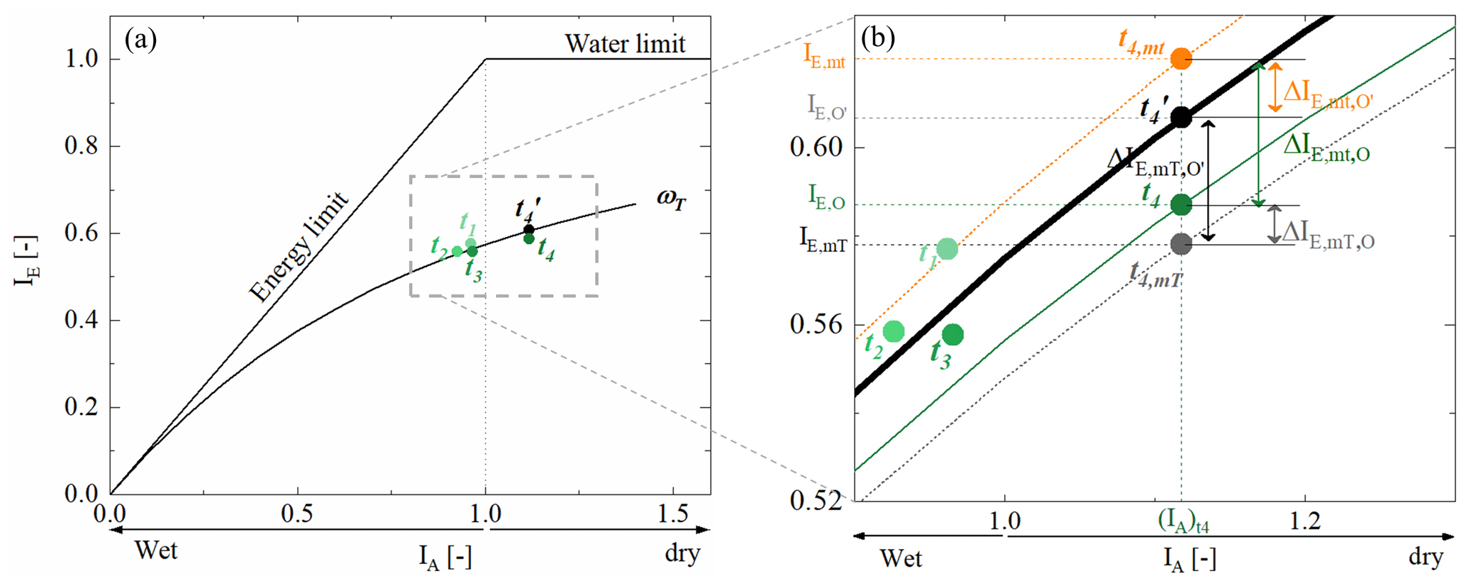
Figure 6(a) Green dots from the light dot to the dark dot indicate the observed positions for the four sub-time periods t1–t4. The black dot indicates the expected location on the parametric Budyko curve with ωT derived from the entire observed time period. We select time period t4 as an example to present the modelled positions in the zoom-in plot (b). The grey dot t4,mT indicates the modelled position based on Scenario 1, which is with , and the orange dot t4,mt indicates the modelled position based on Scenario 2, which is with . (black arrow) indicates the deviation between the modelled IE,mT based on Scenario 1 and the expected . (orange arrow) indicates the deviation between the modelled IE,mt based on Scenario 2 and the expected . (grey arrow) indicates the deviation between the modelled IE,mT based on Scenario 1 and the observed IE,O. (green arrow) indicates the deviation between the modelled IE,mt based on Scenario 2 and the observed IE,O.
5.1 Observed multi-decadal hydro-climatic variability
Based on the initial analysis of water balance data for the four sub-time periods, significant differences were observed in the variability of different hydro-climatic indicators over the 1953–2022 study period (Fig. 3). While periods t1 and t4 were characterized by rather low mean annual precipitation of ∼ 870 and 811 mm yr−1, respectively, periods t2 and t3 were subject to, on average, higher precipitation of ∼ 911 mm yr−1. While summer precipitation remained rather stable over the study period (Fig. 3f), the above was mostly caused by fluctuations in winter precipitation (Fig. 3k). In contrast, potential evaporation EP has gradually increased by 7 % from 836 to 906 mm yr−1 (Fig. 3b). Similarly reflecting increases in temperature (Fig. 3b), the annual snowpack and associated snowmelt have continuously decreased from around 98 mm yr−1 to around 50 mm yr−1 between t1 and t4 (Fig. 3c). A slight decrease in the number of days with precipitation from ∼ 264 to 251 (Fig. 3d), on average, mostly due to changes in the summer months (Fig. 3n), was accompanied by some rather limited variability in precipitation intensities (Fig. 3e), mostly during winter (Fig. 3j). Overall, the comparatively humid periods t1–t3 that were characterized by IA fluctuating between 0.93 and 0.97 were followed by a markedly more arid period t4 with IA = 1.12 (Table 2, Fig. 6). In response to the multi-decadal variability in IA, expressed as movement along the x axis in the Budyko framework, the catchment experienced IE varying between 0.56 and 0.59 (Table 2, Fig. 6). However, this observed variability was somewhat lower than the variability IE,ωT = 0.55–0.61 that would have been expected based on ωT. This illustrates that the hydrological response did not consistently follow its long-term trajectory defined by ωT. Instead, deviations from the expected positions, and thus values of that are different to ωT, were observed for the individual periods. More specifically, the deviations gradually decreased from = 0.01 in t1 to = −0.02 in t4 (Fig. 6). This systematic shift towards lower (more negative) and thus also lower indicates that, at the same IA, a smaller fraction of precipitation is released as evaporation, i.e. IE, now than at the start of the 70-year study period. Although the magnitude of deviations of ± 0.02 remains rather minor, similar to what was recently reported elsewhere (Ibrahim et al., 2024; Tempel et al., 2024), their systematic shift in particular to one direction implies that changes in the system other than IA have a visible effect on the hydrological response pattern.
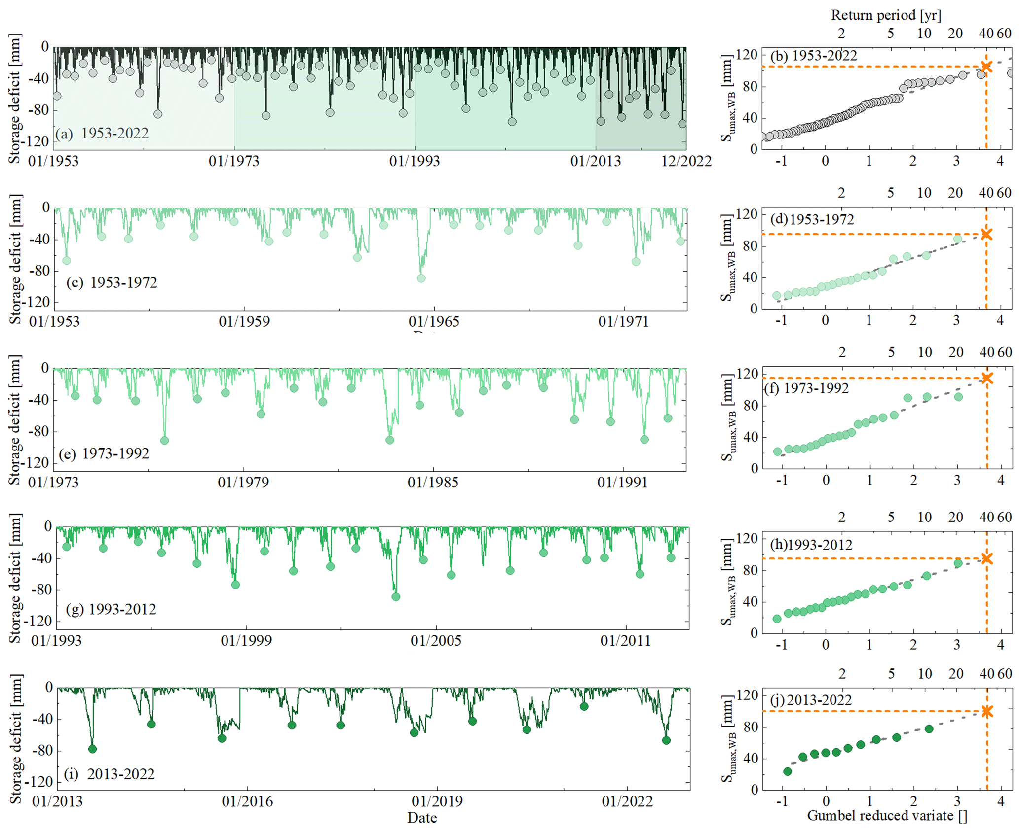
Figure 7The time series of storage deficits as calculated by Eq. (7) for the entire time period T (1953–2022) and for the four sub-time periods (green shades from light to dark for the time period from t1 to t4) (a, c, e, g, and i). The maximum annual deficits are indicated by the dots. Estimation of Sumax as the storage deficit associated with a 40-year return period using the Gumble extreme value distribution for different time periods (b, d, f, h, and j). The orange crosses indicate the values of Sumax for the different time periods.
5.2 Root zone storage capacity Sumax,WB estimated from water balance data
As the baseline of our study, the annual maximum storage deficits fluctuate between 97 mm in 2022 and 16 mm in 1970 (Fig. 7a). Assuming an adaptation to dry spells with 40-year return periods, the root zone storage capacity over the entire 1953–2022 study period (Scenario 1) was estimated to be = 105 mm (Table 2, Fig. 7b). In the next step, the storage deficits and the associated root zone storage capacity for each period from t1 to t4 were estimated (Scenario 2). and for periods t1 and t3, respectively, are estimated at the same value of 95 mm. In contrast, and somewhat counterintuitively, the highest value over the study period is found in the wettest period (t2) and reaches = 115 mm, while the driest period (t4) is characterized by = 100 mm (Table 2, Fig. 7c–j). These patterns suggest that Sumax,WB did vary by ∼ 20 mm, equivalent to ∼ 20 % throughout the 1953–2022 period. In contrast to , which was characterized by a systematic shift towards more negative deviations over time, no evidence was found of a systematic, one-directional shift in Sumax,WB. Instead, Sumax,WB evolved following a somewhat cyclic pattern.
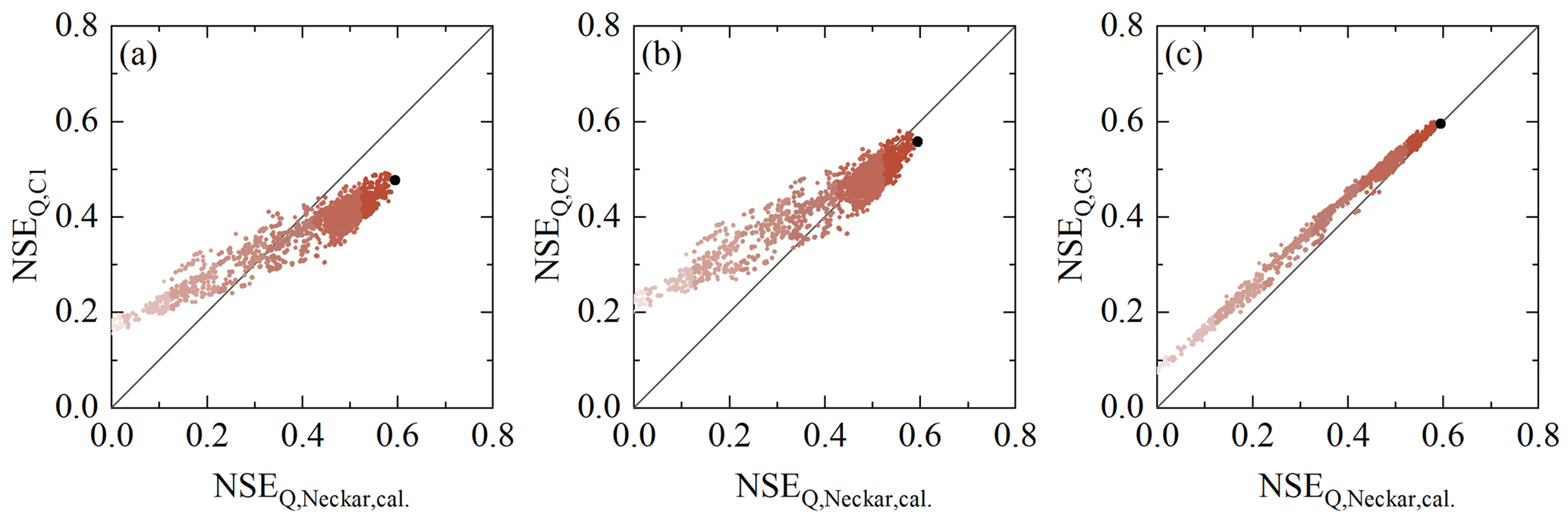
Figure 8Selected model performance metrics in the entire time period 1 January 1953–31 December 2022 of the upper Neckar River basin against the model performance in uncalibrated sub-catchment-based (C1: Rottweil; C2: Plochingen at the Fils River; C3: Horb) parameter sets derived from the calibration for the entire time period. The dots indicate all the Pareto optimal solutions in the multi-objective model performance space. The shades from dark to light indicate the overall model performance based on the Euclidean distance DE, with the black solutions representing the overall better solutions (i.e. larger DE).
5.3 Root zone storage capacity Sumax,cal estimated as a calibration parameter
5.3.1 Model calibration for 1953–2022 (Scenario 1)
The model parameter sets determined as feasible after calibration over the entire 1953–2022 study period in Scenario 1 reproduce the main features of the hydrological response (Fig. 2d). More specifically, the modelled hydrographs in particular describe the timing of high flows well while somewhat underestimating the flow peaks for the best-performing model in terms of DE (Eq. 9). The low flows and the shapes of the recessions are generally captured well (NSElog Q = 0.67). Crucially, the model also reproduces the other observed streamflow signatures well, e.g. the flow duration curves (NSElog FDC = 0.96), the autocorrelation function (NSEAC = 0.99), and the long-term and seasonal runoff coefficients ( = 0.90, = 0.83, and = 0.91). The latter further implies that the modelled long-term actual evaporative fluxes EA (Fig. 2b) and thus IE,ωT are, on average, consistent with the observed ones, which can be seen in Fig. 6. The model, calibrated on the overall response of the upper Neckar River basin, also exhibited considerable skill in representing spatial differences in the hydrological response by reproducing observed streamflow in the three sub-catchments (C1–C3) similarly well (Fig. 8) without any further recalibration. The overall model skill to mimic the hydrological response corresponds well to a similar implementation of the model in the greater study area by Wang et al. (2023). A detailed list of the performance metrics is provided in Table S4 in the Supplement.
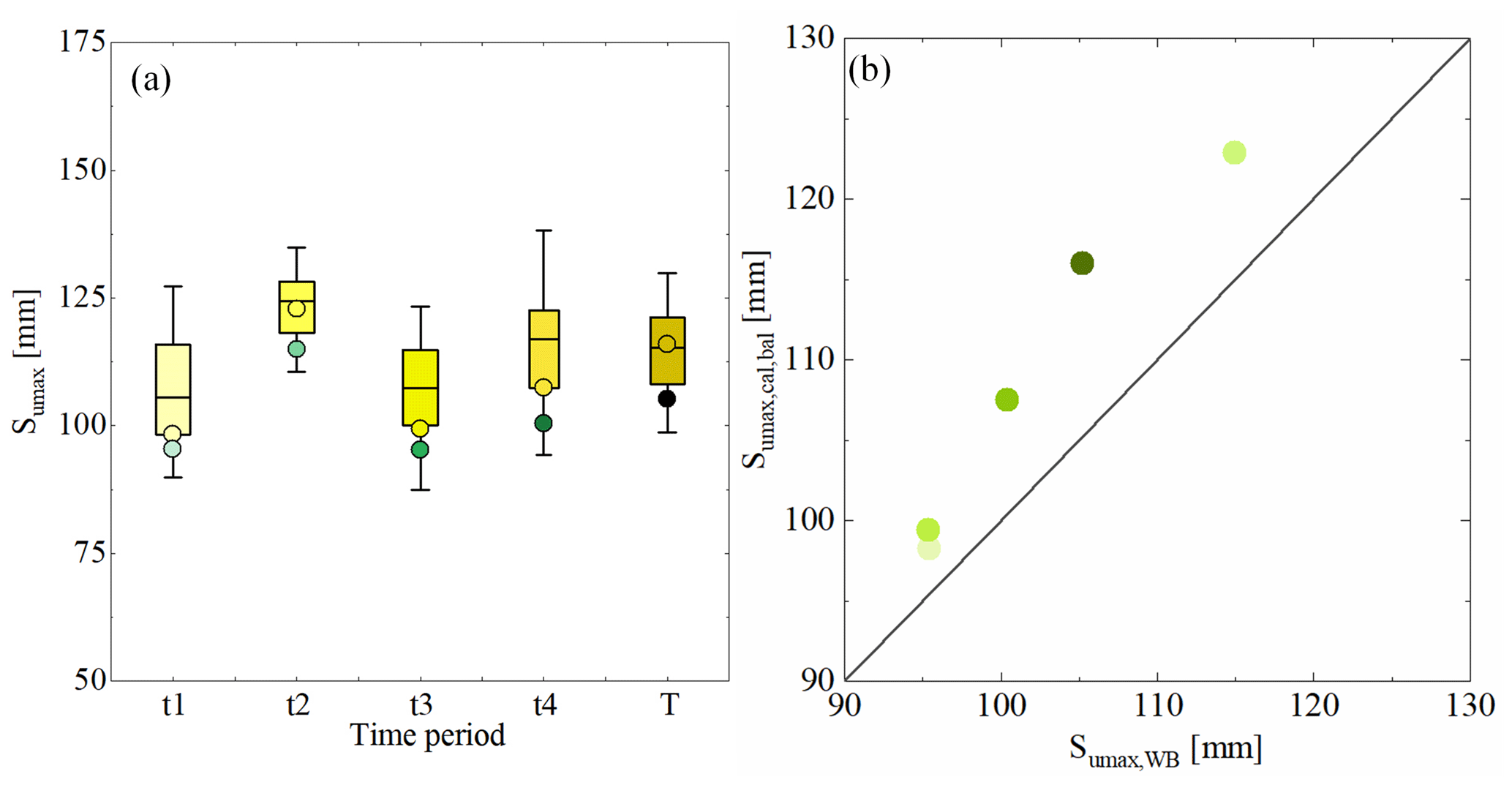
Figure 9(a) Sumax values derived from the water balance method and the hydrological model for different time periods. The yellow boxes from light to dark indicate the range of Sumax,cal for the sub-time period from t1 to t4 and the entire time period T based on the corresponding parameter sets derived from the model. Yellow dots indicate the corresponding based on the most balanced solution, and green dots indicate the corresponding Sumax,WB derived from the water balance method. (b) Values of against Sumax,WB. The yellow–green dots from light to dark indicate the values of Sumax for the sub-time period from t1 to t4 and the entire time period T.
The model calibration resulted in pronounced differences in the root zone storage capacity parameters for three individual landscape classes. While for forest-dominated land it was estimated at Sumax,F = 158 mm for the best-performing model (5th and 95th percentiles of all feasible solutions: 138–168 mm), it reached Sumax,G = 95 mm (5th and 95th percentiles: 71–123 mm) for grassland/cropland and Sumax,W = 61 mm for wetland (5th and 95th percentiles: 49–68 mm), which reflects differences in the vegetation type and position in the landscape (Fan et al., 2017). Remarkably, the catchment root zone storage capacity, estimated by aggregating the individual values according to their areal fractions, at Sumax,cal = 116 mm (5th and 95th percentiles: 99–130 mm; Fig. 9a) came very close to the estimate of Sumax,WB = 105 mm that is directly derived from the water balance method without any calibration, as described in Sect. 5.2.
5.3.2 Model calibration for the individual periods t1–t4 (Scenario 2)
The model parameter sets obtained from the individual calibration for each period from t1 to t4 reproduce the hydrographs of the corresponding periods as well or slightly better than when using the long-term average parameters from Scenario 1 (see the detailed performance metrics in Table S4). In particular, the runoff coefficients of ∼ 0.86–0.91, ∼ 0.84–0.90, and ∼ 0.88–0.92 could be mimicked rather well. Similarly, the daily dynamics with NSElog Q ∼ 0.63–0.72 for the best-performing model of each period and most other hydrological signatures could be reproduced marginally better.
The individual calibration over each period t1–t4 resulted in associated differences in the catchment-scale root zone storage capacity of each period. Based on the best-performing models, the calibrated values varied between low values for t1 and t2, with = 98 mm and = 99 mm, and higher values for the other two periods, with = 122 mm and = 107 mm (Table 2, Fig. 9a). The magnitudes of obtained by calibration in the individual time periods t1–t4 are, with a difference of 5 mm (∼ 5 %), on average very close to the estimated on the basis of the water balance for the same periods. Perhaps even more notably, the temporal evolution of and follows the same sequence over time (R2 = 0.95, p = 0.05; Fig. 9b).
5.4 Effect of Sumax on temporal fluctuation in the trajectories of the Budyko curve
The deviations between the expected evaporative index and the observed evaporative index IE,O for all the periods t1–t4 become gradually more negative from t1 ( = 0.013) to t4 ( = −0.020), which is consistent with decreases in and downward shifts of the associated parametric Budyko curves over time as described in Sect. 5.1. These systematic reductions in over the 70-year study period are not reflected in the fluctuations of root zone storage capacities, irrespective of how they were estimated, i.e. (p = 0.85) or (p = 0.96), as illustrated in Fig. 10.
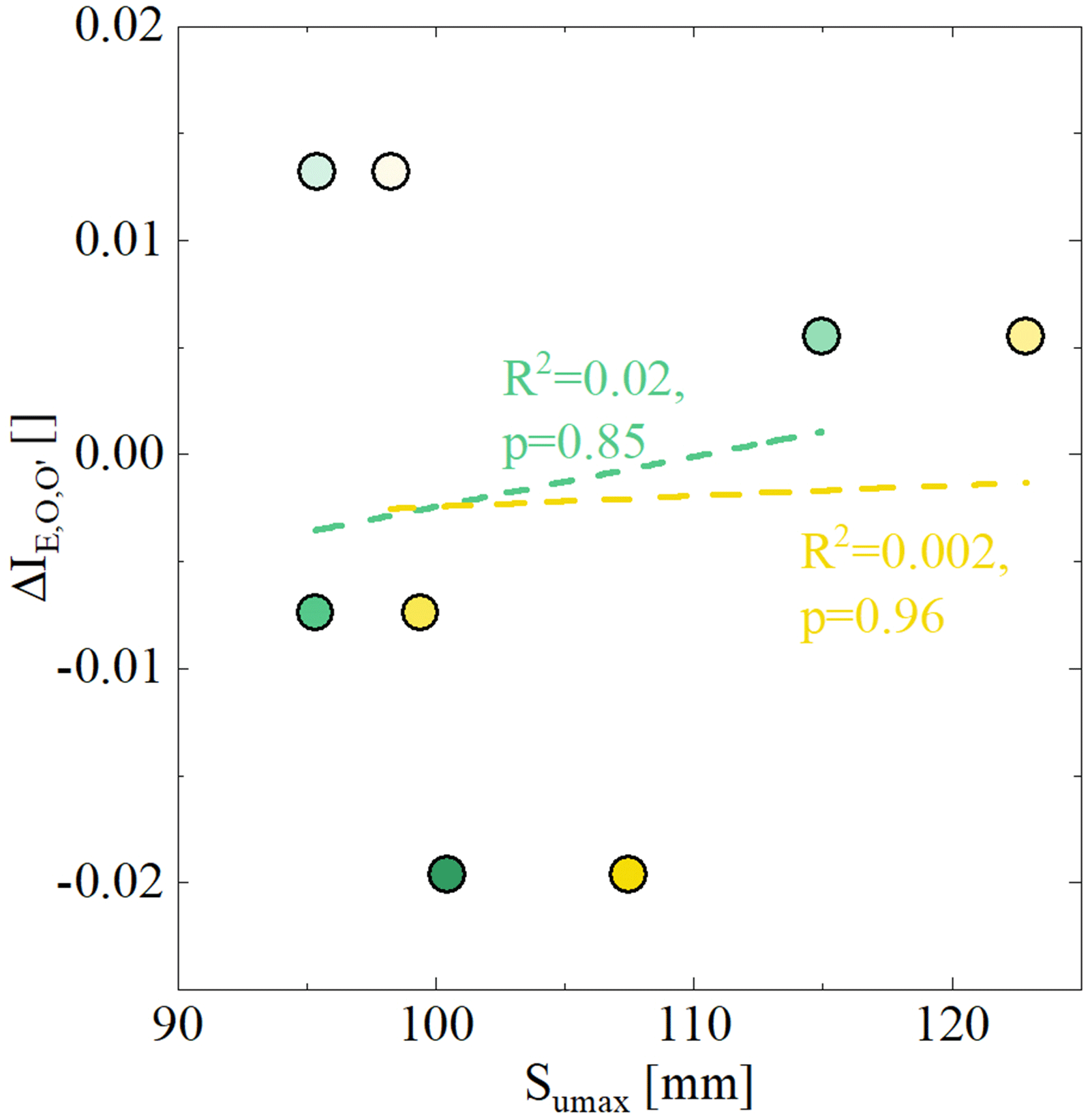
Figure 10Relationships between the deviations and the values of Sumax,WB and Sumax,cal for the four sub-time periods (t1–t4) which are derived from the water balance method (green circles) and the hydrological model calibration (yellow circles), respectively.
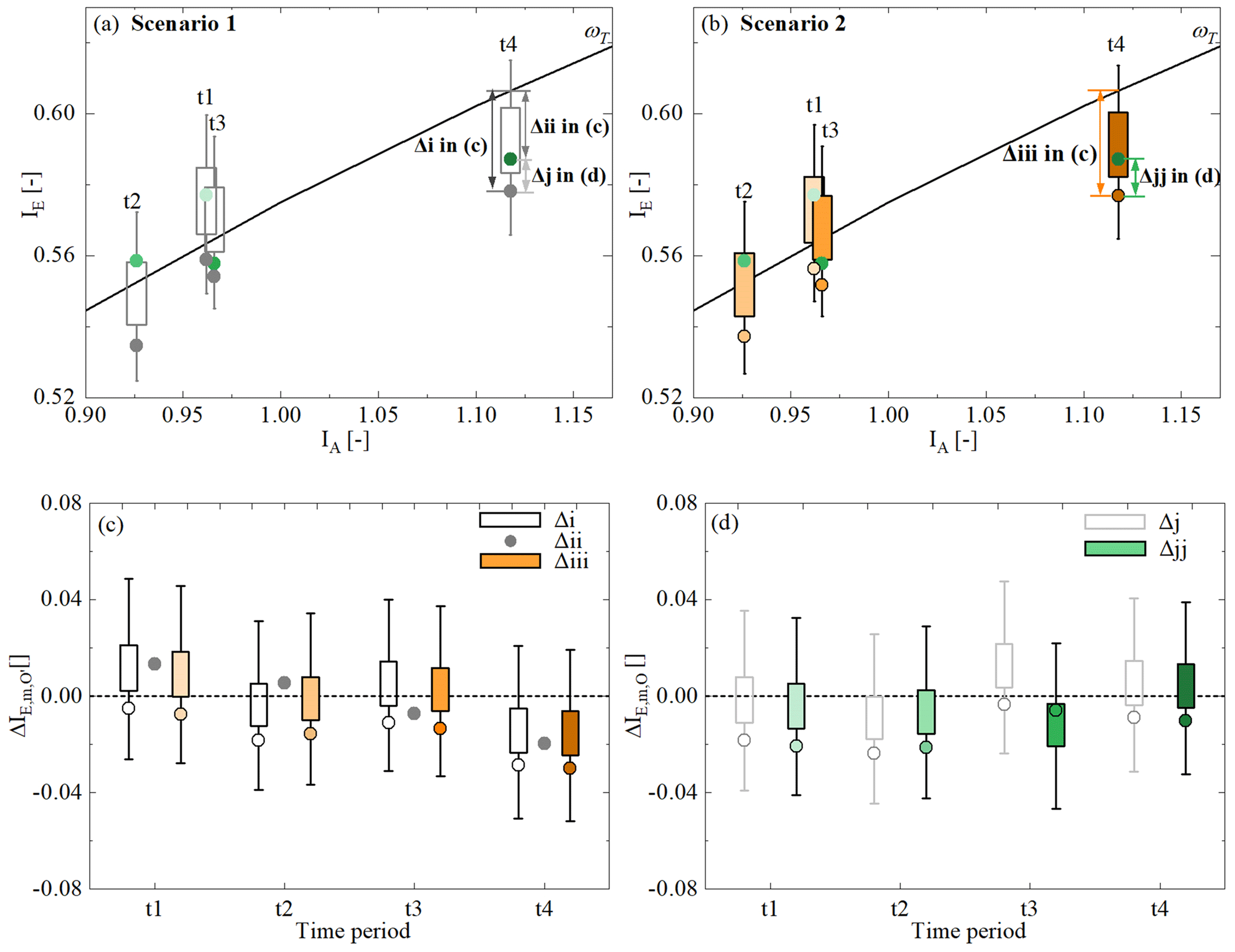
Figure 11(a) The grey boxes (IE,mT) indicate the modelled evaporative index based on all the Pareto front solutions for the four sub-time periods based on Scenario 1 with a stationary and grey dots based on the most balanced solution based on Scenario 1. The green circles from light to dark in panels (a) and (b) indicate the observed evaporative index for the four sub-time periods from t1 to t4. (b) The orange circles (IE,mt) indicate the modelled evaporative index based on all the Pareto front solutions for the four sub-time periods (from lighter to darker shades) based on Scenario 2 with time-variant and the orange circles based on the most balanced solution for Scenario 2. The black boxes in panel (c) indicate the deviations = IE,mT − (Δ i) based on all the Pareto front solutions for the four sub-time periods and the dark-grey circles based on the most balanced solution based on Scenario 1. The orange boxes in panel (c) indicate the deviations = IE,mt − (Δ iii) based on all the Pareto front solutions for the four sub-time periods and the orange circles based on the most balanced solution for Scenario 2. The grey dots indicate the deviation (Δ ii) between the observed IE,O for each sub-time period and the corresponding expected . The light-grey boxes in panel (d) indicate the deviations = IE,mT − IE,O (Δ j) based on all the Pareto front solutions for the four sub-time periods and the grey circles based on the most balanced solution. The green boxes in panel (d) indicate the deviations = IE,mt − IE,O (Δ jj) based on all the Pareto front solutions for the four sub-time periods and the green circles based on the most balanced solution.
The above is further corroborated by comparing the modelled IE from Scenarios 1 and 2 for each period t1–t4. More specifically, in Fig. 11c it can be seen that Scenario 1, based on a time-invariant, long-term average obtained over the entire 1953–2022 period generates deviations from the expected long-term average for each period t1–t4. In this case, the modelled IE does not follow the expected . However, nor does it follow the sequence of increasingly negative deviations from 0.013 in t1 to −0.020 in t4 as observed in reality (). Instead, remains negative for all the time periods and fluctuates between = −0.005 and −0.029 (white boxplots in Fig. 11c). Replacing the time-invariant with an individual for each period t1–t4 in Scenario 2 accounts for the different effects of vegetation in the individual periods. If Sumax controlled the observed deviations from the expected , Scenario 2 would generate estimates of that are closer to the observed ones than those of Scenario 1. However, no evidence was found of that: the deviations obtained by Scenario 2 with time-variable Sumax for each period t1–t4 are largely indistinguishable (orange boxplots in Fig. 11c) from those generated by Scenario 1 with time-invariant Sumax. As a consequence, the evaporative index IE modelled with time-variable is not found to be closer to the observed IE for Scenario 2 than for Scenario 1. On the contrary, the deviations from the observed IE obtained from the time-invariant Scenario 1 are in most time periods, albeit only slightly, less pronounced (Fig. 11d).
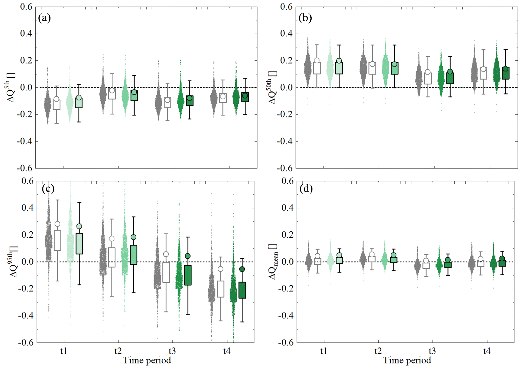
Figure 12The relative errors of observed and modelled high (Q5th), median (Q50th), and low (Q95th) flow quantiles and the mean Q for different time periods based on two scenarios. The grey shades and the corresponding dots indicate the relative errors based on Scenario 1 with all the Pareto front solutions, and the grey circles indicate the most balanced solution. The corresponding values for Scenario 2 are shown in green.
5.5 Effect of Sumax on streamflow
Corresponding to the above findings, there is no significant difference in the modelled average streamflow between Scenario 1, using the long-term average Sumax, and Scenario 2, using individual Sumax values for each time period (Fig. 12d). While the model for both scenarios consistently and similarly underestimates high flows (Q5th, Fig. 12a) by ∼ 10 %, it overestimates median flows by ∼ 15 % with both time-invariant and time-variable Sumax for all time periods (Fig. 12b). Interestingly, the low flows are overpredicted by ∼ 10 %–20 % in the first two periods, while they are underpredicted by up to ∼ 20 % in the later periods in both scenarios (Fig. 12c). In addition, it was also found that using a time-variable Sumax in Scenario 2 did not have any discernible effect on the seasonal flow pattern (not shown). The fact that both scenarios generate similar estimates over different flow percentiles and, in particular, that the time-variable Scenario 2 reflects the same systematic shift in the ability of the model to reproduce low flows as Scenario 1 suggests, together with the very minor effects of the time-variable Sumax in Scenario 2 on the model performance metrics, that the adaptation of Sumax to changing climatic conditions does not significantly affect the average hydrological response pattern in the Neckar River basin.
6.1 Multi-decadal changes in root zone storage capacity Sumax
As Gao et al. (2024) suggested, considering the terrestrial ecosystem structure can improve our understanding of hydrological processes and how the ecosystem can survive and be developed. It is valuable to explore how ecosystems adapt to climatic variability (which is reflected in fluctuations in Sumax) and how this affects the long-term partitioning of drainage, evaporation, and hydrological response. This study is the first to systematically and explicitly quantify how the root zone storage capacity Sumax changes with changing climatic conditions over time. The values of root zone storage capacity, estimated from both water balance data and as a model calibration parameter, indeed show significant and corresponding fluctuations over multiple decades, varying by up to ±20 %. At Sumax ∼ 95–115 mm, the overall estimated magnitudes fall well within the range of long-term average values reported previously for the greater region (e.g. Bouaziz et al., 2021; Hrachowitz et al., 2021; Tempel et al., 2024) and other temperate, humid environments (e.g. Kleidon, 2004; Gao et al., 2014b; de Boer et al., 2016; Wang-Erlandsson et al., 2016; Stocker et al., 2023; van Oorschot et al., 2024).
The values of Sumax obtained from both methods are very similar and within an error margin of only ∼ 5 %. In addition, they both follow a comparable change over time. Together, this lends support to the underlying assumption that this temporal evolution of Sumax may indeed be a fingerprint of vegetation adaptation to changing climatic conditions. More specifically, as Sumax,WB is explicitly based on the estimates of transpiration Er (Eq. 9), it could be plausibly argued that during specific years only more water is used for Er but that the size of the water storage volume accessible for roots may not necessarily change. In that case, changes in Sumax,WB would not reflect actual changes in the active root system but only in how much water was used by them. In contrast, Sumax,cal inferred as a calibration parameter of a hydrological model regulates not only transpiration, but, critically, also the generation of streamflow. If therefore the active root system in reality did not change and fluctuations in Sumax,WB were a mere artifact of changes in water uptake from a fixed-size volume instead of an actual change in maximum vegetation-accessible sub-surface water volumes, fluctuations in Sumax,cal would not mirror those of Sumax,WB, and the use of Sumax,WB in the hydrological model would, due to the non-linear character of the flow generation function in the model (Eq. S20 in Table S1), lead to misrepresentations of streamflow dynamics. However, no deteriorations of the model performance with a changing Sumax were found here. Even more, the fact that Sumax,WB and Sumax,cal are characterized by very similar magnitudes and fluctuations adds further evidence that their evolution over time is a manifestation of vegetation adapting its active root system to changing climatic conditions.
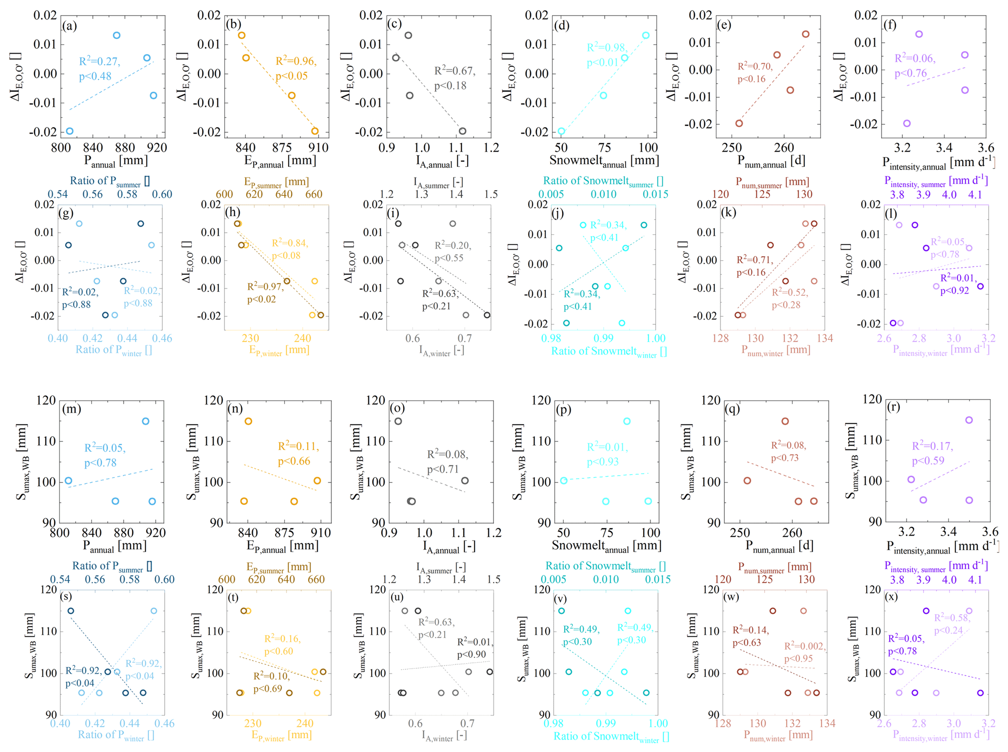
Figure 13Relationships between the temporal fluctuation of the deviations (, black dots in Fig. 10a), Sumax,WB, and climate indices, including precipitation (P), potential evaporation (EP), the aridity index (IA), the estimated snowmelt water (Snowmelt), the number of precipitation days (Pnum), and the precipitation intensity (Pintensity) for the four sub-time periods. Relationships between the temporal fluctuation of the deviations (, black dots in Fig. 10a) and the climate indices for the four sub-time periods are shown in the first two rows in panels (a–l) (i.e. (a–f) vs. annual climatic indices and (g–l) vs. seasonal climatic indices). Relationships between the temporal fluctuation of Sumax,WB derived from the water balance method and climate indices for the four sub-time periods are shown in the last two rows in panels (m–x) (i.e. (m–r) Sumax,WB vs. annual climatic indices and (s–x) Sumax,WB vs. seasonal climatic indices).
Several previous studies in similar environments found that the root zone storage capacity Sumax can decrease by 50 % or more after deforestation and that these changes not only cause reductions in IE by −0.2 or more, which reflect changes in ω and thus the overall functioning of the system, but also influence hydrological dynamics on short timescales, such as the magnitudes of flow peaks (Nijzink et al., 2016a; Hrachowitz et al., 2021). In contrast to the above studies, the ±20 % fluctuations of Sumax here did not lead to similarly marked shifts in IE or ω. This is further corroborated by an analysis of different variables as potential controls on Sumax and ΔIE as shown in Fig. 13. Fluctuations of Sumax can to a large extent be attributed to the variability in the ratio of winter precipitation to summer precipitation (Fig. 13s) as a simplified metric for precipitation seasonality. This comes as no surprise, as the computation of Sumax,WB is explicitly based on the seasonal water deficit (Eq. 7). It merely shows that, when more precipitation falls in summer, at a time when evaporative demand is highest, the lower Sumax needs to provide vegetation with sufficient and continuous access to water for continuous vegetation transpiration. All the other tested variables do not exert any major influence on Sumax in the study region. Conversely, it was found that the deviations ΔIE are largely independent of the seasonality of precipitation (Fig. 13g). Instead, increases in summer EP are correlated with decreases in ΔIE (Fig. 13h) and thus with a reduction in ET. The observed systematic shift towards a more negative ΔIE, which indicates proportionally less evaporation, thus coincides with the gradually increasing summer EP over time. This points towards different controls on ΔIE than on Sumax and the potential role of increased vegetation water stress in summer as the main driver of ΔIE. Thus, while there is compelling evidence of fluctuations in Sumax, the above illustrates that these changes cannot explain the observed deviations from the expected long-term Budyko trajectory in the study region.
It is also important to note that the temporal fluctuations of both Sumax and ΔIE can be subject to uncertainties. In spite of the findings reported by Han et al. (2020) that, for most river catchments worldwide, ∼ 0 holds over averaging periods similar to the ones used here (t1–t4), this assumption may not completely hold in the study region. In relation to this, we did not consider potential effects of unobserved groundwater import or export on the long-term water balance either (Bouaziz et al., 2018).
As only < 2 % of the study area experienced documented land use change over the 1953–2022 period and no major reservoirs are present upstream of the study basin outlet, here we interpret fluctuations in Sumax as being a reflection of adaptations of root systems to changing hydro-climatic conditions. However, some of the fluctuations may be a consequence of land management practices not quantified by available gridded land cover products such as CORINE, including forest thinning (Hrachowitz et al., 2021) or rejuvenation (Teuling and Hoek van Dijke, 2020). In addition, although here we mainly attribute changes in Sumax to changes in root systems, these may be complemented by additional effects of changes in vegetation water use due to feedbacks with increases in atmospheric CO2 (e.g. Berghuijs et al., 2017; Jaramillo et al., 2018).
6.2 Effect of changing Sumax on the representation of streamflow in a model
Reflecting their lack of explanatory power for the changes in ΔIE, our results correspondingly indicate that signatures of both annual flow, such as the average Q5th, Q50th, or Q95th, and seasonal flow are not reproduced better by the hydrological model when replacing a time-invariant, long-term average Sumax with a temporally dynamic Sumax. Overall, these results are in contrast to previous studies that quantified the effect of a time-variable Sumax parameter following deforestation. For example, Nijzink et al. (2016a) reported that adjusting the parameter Sumax to a lower value improves a model's ability to reproduce streamflow after deforestation. These findings were strongly supported by Hrachowitz et al. (2021), who found that post-deforestation model recalibration resulted in a lower Sumax and a significantly better performance compared to using parameters from pre-deforestation calibration. However, our results are also different from those reported by Duethmann et al. (2020), who found that accounting for vegetation dynamics in a model in the form of changing surface resistances to vegetation improved the long-term performance of the model. Similarly, Bouaziz et al. (2022) estimated the future Sumax based on projected future hydro-climatic conditions. In a somewhat more humid environment, they found that an estimated ∼ 25 % future increase in Sumax from ∼ 170 to 226 mm may lead to reductions in the mean and maximum annual Q of ∼ 5 %. More pronounced effects were reported on the intra-annual timescale, with reductions in autumn and winter Q of up to ∼ 15 %. This was accompanied by increases of up to ∼ 15 % in summer evaporation and decreases of 10 % in winter groundwater levels. Irrespective of the additional uncertainties in their study introduced by future projections, the much less pronounced effects we found in our analysis are most likely a consequence of the lower absolute magnitude of Sumax that remains below 115 mm in the study region. These lower Sumax values reflect lower storage requirements in summer, due to a precipitation pattern in the Neckar River basin that is more evenly spread throughout the year. In other words, the fact that here ∼ 55 %–60 % of the annual precipitation falls in summer (Fig. 3f and k) when it is needed most by vegetation due to high EP removes the need for a larger Sumax as a water storage buffer to allow vegetation to survive. However, the lower the magnitude of Sumax, the more frequently storage deficits can be overcome by even rather small rainstorms and the less water is (or needs to be) stored. Thus, even if the relative changes are similar between Bouaziz et al. (2022) and Tempel et al. (2024) in a somewhat more humid environment and our study, abundant summer precipitation causes absolute Sumax fluctuations of less than ±20 mm over time in the Neckar catchment. This in turn limits the influence of the changes on the hydrological response, which has wider implications for the use of models in the Neckar River basin and potentially in other temperate regions with similar hydro-climatic characteristics. More specifically, it has been argued that a changing climate will affect the properties of terrestrial hydrological systems (e.g. Stevens et al., 2020). As these properties are represented by typically time-invariant parameters in hydrological or land surface models, accounting for changing system properties with time-variable formulations of parameters may facilitate more reliable predictions. For many model parameters such a time-variable formulation to estimate their future values is not trivial due to frequently insufficient data and a general lack of mechanistic understanding of the underlying processes. The estimation of Sumax and its temporal evolution based on observed historical or projected future water balance data opens up an opportunity to estimate its magnitude under future conditions for use in models. However, in contrast to the findings in other regions (e.g. Merz et al., 2011) and as discussed above, adapting Sumax to changing conditions in the Neckar River basin does not lead to improved modelled representations of the hydrological response. It is therefore plausible to assume that the use of a time-variable parameter Sumax does not substantially improve future predictions and is thus not necessarily required for at least the next few decades to come and that the use of a long-term average Sumax, obtained either by calibration or based on the water balance, is sufficient in the Neckar River basin and in hydro-climatically similar regions. This in itself is already an interesting finding as it gives modellers process-based evidence that the use of a time-invariant Sumax as a model parameter will also be sufficient for meaningful hydrological predictions in the near future in such an environment. However, it can also be expected that, in more arid regions with less summer precipitation and generally higher Sumax (see e.g. Gao et al., 2014b; Stocker et al., 2023), changes in Sumax will play a more prominent role.
The catchment-scale root zone storage capacity (Sumax) is a critical factor reflecting the moisture exchange between land and atmosphere as well as the hydrological response in terrestrial hydrological systems. However, as a major knowledge gap, it is unclear whether Sumax at the catchment scale evolves over time, reflecting vegetation adaptation to changing climatic conditions. As a consequence, it also remains unclear how potential changes in Sumax may affect the partitioning of water fluxes and, as a consequence, the catchment-scale hydrological response. In this study, for the upper Neckar catchment, based on long-term daily hydrological data (1953–2022), we quantify and analyse how Sumax dynamically evolves over multiple decades, reflecting vegetation adaptation to climate variability and the effects on the hydrological system.
The main findings of our analysis are the following:
-
Sumax has fluctuated by ±20 % between 95 and 115 mm, in response to climatic variability over the 70-year study period.
-
Estimates of Sumax obtained from both methods, i.e. based on water balance data and model calibration parameters, respectively, were, with differences of ∼ 5 %, highly consistent with each other and correlated in time (R2 = 0.95, p = 0.05). Findings (1) and (2) support the hypothesis that Sumax, even in temperate, humid climates such as in the Neckar River basin, significantly changes over multiple decades, reflecting vegetation adaptation to climatic variability.
-
The estimated fluctuations of Sumax were inconsistent with the temporal sequence of observed deviations ΔIE ∼ ± 0.02 from the expected IE over the study period (R2 = 0.02, p = 0.85).
-
As a consequence, replacing a long-term average, time-invariant parameter Sumax in a hydrological model with a time-variable formulation of Sumax does not lead to a better representation of the observed ΔIE. Based on (3) and (4), the hypothesis that Sumax affects the long-term partitioning of drainage and evaporation and thus controls deviations ΔIE from the catchment-specific trajectory in the Budyko space needs to be rejected for the Neckar River basin.
-
Replacing the time-invariant Sumax with a time-variable Sumax in the hydrological model leads to only very minor improvements of the model to reproduce streamflow dynamics. The hypothesis that a time-dynamic implementation of Sumax improves the representation of streamflow in the hydrological model therefore also needs to be rejected for the Neckar River basin.
Overall, our study is the first to systematically document the temporal evolution of Sumax, and although limited to the Neckar River basin, it provides clear quantitative evidence that Sumax can significantly change over multiple decades, reflecting vegetation adaptation to climate variability. However, these changes do not cause deviations from the long-term average Budyko curve under changing climatic conditions. This implies that the temporal evolution of Sumax does not control variation in the partitioning of water fluxes and has no significant effects on fundamental hydrological response characteristics of the upper Neckar River basin. As the use of time-variable Sumax over the 70-year study period does not improve the performance of the hydrological model, it can plausibly be assumed that in the study region the use of time-invariant Sumax as a model parameter will be sufficient for meaningful predictions over at least the next few decades.
The model codes underlying this paper are available online in the 4TU data repository (DOI: https://doi.org/10.4121/922d30de-a26b-4c81-8644-ad036182239c, Wang and Hrachowitz, 2024). The equations used in the model are described in the Supplement The meteorological and hydrological data used in this study can be obtained from the German Weather Service (DWD) (https://opendata.dwd.de/climate_environment/CDC/observations_germany/climate/daily/more_precip/historical/, DWD, 2024) and the German Federal Institute of Hydrology (BfG) (https://portal.grdc.bafg.de/applications/public.html?publicuser=PublicUser#dataDownload/Stations, BfG, 2024).
The supplement related to this article is available online at: https://doi.org/10.5194/hess-28-4011-2024-supplement.
SW, MH, and GS designed the study. SW performed the experiments. All the authors contributed to the general idea, the discussion, and the writing of the manuscript.
At least one of the (co-)authors is a member of the editorial board of Hydrology and Earth System Sciences. The peer-review process was guided by an independent editor, and the authors also have no other competing interests to declare.
Publisher's note: Copernicus Publications remains neutral with regard to jurisdictional claims made in the text, published maps, institutional affiliations, or any other geographical representation in this paper. While Copernicus Publications makes every effort to include appropriate place names, the final responsibility lies with the authors.
We gratefully acknowledge the financial support from the China Scholarship Council (CSC).
This research has been supported by the Chinese Research Council (grant no. 202006190030).
This paper was edited by Fuqiang Tian and reviewed by Lele Shu and two anonymous referees.
AghaKouchak, A., Feldman, D., Hoerling, M., Huxman, T., and Lund, J.: Water and climate: Recognize anthropogenic drought, Nature, 524, 409–411, https://doi.org/10.1038/524409a, 2015.
Ajami, N. K., Gupta, H., Wagener, T., and Sorooshian, S.: Calibration of a semi-distributed hydrologic model for streamflow estimation along a river system, J. Hydrol., 298, 112–135, https://doi.org/10.1016/j.jhydrol.2004.03.033, 2004.
Alila, Y., Kuraś, P. K., Schnorbus, M., and Hudson, R.: Forests and floods: A new paradigm sheds light on age-old controversies, Water Resour. Res., 45, W08416, https://doi.org/10.1029/2008WR007207, 2009.
Bahremand, A. and Hosseinalizadeh, M.: Development of conceptual hydrological FLEX-Topo model for loess watersheds influenced by piping and tunnel erosion in Golestan Province of Iran, Journal of Water and Soil Conservation, 29, 115–133, https://doi.org/10.22069/jwsc.2022.20050.3544, 2022.
Berghuijs, W. R. and Woods, R.: A simple framework to quantitatively describe monthly precipitation and temperature climatology, Int. J. Climatol., 36, 3161–3174, https://doi.org/10.1002/joc.4544, 2016.
Berghuijs, W. R., Larsen, J. R., Van Emmerik, T. H., and Woods, R. A.: A global assessment of runoff sensitivity to changes in precipitation, potential evaporation, and other factors, Water Resour. Res., 53, 8475–8486, https://doi.org/10.1002/2017WR021593, 2017.
BfG: Streamflow datasets in Germany, BfG [data set], https://portal.grdc.bafg.de/applications/public.html?publicuser=PublicUser#dataDownload/Stations, last access: 27 August 2024.
Bouaziz, L., Weerts, A., Schellekens, J., Sprokkereef, E., Stam, J., Savenije, H., and Hrachowitz, M.: Redressing the balance: quantifying net intercatchment groundwater flows, Hydrol. Earth Syst. Sci., 22, 6415–6434, https://doi.org/10.5194/hess-22-6415-2018, 2018.
Bouaziz, L. J., Steele-Dunne, S. C., Schellekens, J., Weerts, A. H., Stam, J., Sprokkereef, E., Winsemius, H. H., Savenije, H. H., and Hrachowitz, M.: Improved understanding of the link between catchment-scale vegetation accessible storage and satellite-derived Soil Water Index, Water Resour. Res., 56, e2019WR026365, https://doi.org/10.1029/2019WR026365, 2020.
Bouaziz, L. J. E., Fenicia, F., Thirel, G., de Boer-Euser, T., Buitink, J., Brauer, C. C., De Niel, J., Dewals, B. J., Drogue, G., Grelier, B., Melsen, L. A., Moustakas, S., Nossent, J., Pereira, F., Sprokkereef, E., Stam, J., Weerts, A. H., Willems, P., Savenije, H. H. G., and Hrachowitz, M.: Behind the scenes of streamflow model performance, Hydrol. Earth Syst. Sci., 25, 1069–1095, https://doi.org/10.5194/hess-25-1069-2021, 2021.
Bouaziz, L. J. E., Aalbers, E. E., Weerts, A. H., Hegnauer, M., Buiteveld, H., Lammersen, R., Stam, J., Sprokkereef, E., Savenije, H. H. G., and Hrachowitz, M.: Ecosystem adaptation to climate change: the sensitivity of hydrological predictions to time-dynamic model parameters, Hydrol. Earth Syst. Sci., 26, 1295–1318, https://doi.org/10.5194/hess-26-1295-2022, 2022.
Brath, A., Montanari, A., and Moretti, G.: Assessing the effect on flood frequency of land use change via hydrological simulation (with uncertainty), J. Hydrol., 324, 141–153, https://doi.org/10.1016/j.jhydrol.2005.10.001, 2006.
Brown, D. G., Johnson, K. M., Loveland, T. R., and Theobald, D. M.: Rural land-use trends in the conterminous United States, 1950–2000, Ecol. Appl., 15, 1851–1863, https://doi.org/10.1890/03-5220, 2005.
Budyko, M. I.: Climate and Life, Academic Press, New York, 508 pp., ISBN 9780080954530, 1974.
Coenders-Gerrits, A. M. J., Van der Ent, R. J., Bogaard, T. A., Wang-Erlandsson, L., Hrachowitz, M., and Savenije, H. H. G.: Uncertainties in transpiration estimates, Nature, 506, E1–E2, https://doi.org/10.1038/nature12925, 2014.
de Boer-Euser, T., McMillan, H. K., Hrachowitz, M., Winsemius, H. C., and Savenije, H. H.: Influence of soil and climate on root zone storage capacity, Water Resour. Res., 52, 2009–2024, https://doi.org/10.1002/2015WR018115, 2016.
Donohue, R. J., Roderick, M. L., and McVicar, T. R.: On the importance of including vegetation dynamics in Budyko's hydrological model, Hydrol. Earth Syst. Sci., 11, 983–995, https://doi.org/10.5194/hess-11-983-2007, 2007.
Donohue, R. J., Roderick, M. L., and McVicar, T. R.: Roots, storms and soil pores: Incorporating key ecohydrological processes into Budyko's hydrological model, J. Hydrol., 436, 35–50, https://doi.org/10.1016/j.jhydrol.2012.02.033, 2012.
Dralle, D. N., Hahm, W. J., Chadwick, K. D., McCormick, E., and Rempe, D. M.: Technical note: Accounting for snow in the estimation of root zone water storage capacity from precipitation and evapotranspiration fluxes, Hydrol. Earth Syst. Sci., 25, 2861–2867, https://doi.org/10.5194/hess-25-2861-2021, 2021.
Duethmann, D., Blöschl, G., and Parajka, J.: Why does a conceptual hydrological model fail to correctly predict discharge changes in response to climate change?, Hydrol. Earth Syst. Sci., 24, 3493–3511, https://doi.org/10.5194/hess-24-3493-2020, 2020.
DWD: Index of /climate_environment/CDC/observations_germany/ climate/daily/more_precip/historical/, DWD [data set], https://opendata.dwd.de/climate_environment/CDC/observations_germany/climate/daily/more_precip/historical/, last access: 27 August 2024.
Efstratiadis, A. and Koutsoyiannis, D.: One decade of multi-objective calibration approaches in hydrological modelling: a review, Hydrolog. Sci. J., 55, 58–78, https://doi.org/10.1080/02626660903526292, 2010.
Ellison, D., Pokorný, J., and Wild, M.: Even cooler insights: On the power of forests to (water the Earth and) cool the planet, Glob. Change Biol., 30, e17195, https://doi.org/10.1111/gcb.17195, 2024.
Euser, T., Hrachowitz, M., Winsemius, H. C., and Savenije, H. H.: The effect of forcing and landscape distribution on performance and consistency of model structures, Hydrol. Process., 29, 3727–3743, https://doi.org/10.1002/hyp.10445, 2015.
Fan, Y., Miguez-Macho, G., Jobbágy, E. G., Jackson, R. B., and Otero-Casal, C.: Hydrologic regulation of plant rooting depth, P. Natl. Acad. Sci. USA, 114, 10572–10577, https://doi.org/10.1073/pnas.1712381114, 2017.
Fenicia, F., Savenije, H. H., Matgen, P., and Pfister, L.: Understanding catchment behavior through stepwise model concept improvement, Water Resour. Res., 44, W01402, https://doi.org/10.1029/2006WR005563, 2008.
Fenicia, F., Savenije, H. H. G., and Avdeeva, Y.: Anomaly in the rainfall-runoff behaviour of the Meuse catchment, Climate, land-use, or land-use management?, Hydrol. Earth Syst. Sci., 13, 1727–1737, https://doi.org/10.5194/hess-13-1727-2009, 2009.
Fu, B.: On the calculation of the evaporation from land surface, Scientia Atmospherica Sinica, 5, 23–31, 1981 (in Chinese).
Gao, H., Hrachowitz, M., Fenicia, F., Gharari, S., and Savenije, H. H. G.: Testing the realism of a topography-driven model (FLEX-Topo) in the nested catchments of the Upper Heihe, China, Hydrol. Earth Syst. Sci., 18, 1895–1915, https://doi.org/10.5194/hess-18-1895-2014, 2014a.
Gao, H., Hrachowitz, M., Schymanski, S., Fenicia, F., Sriwongsitanon, N., and Savenije, H.: Climate controls how ecosystems size the root zone storage capacity at catchment scale, Geophys. Res. Lett., 41, 7916–7923, https://doi.org/10.1002/2014GL061668, 2014b.
Gao, H., Hrachowitz, M., Wang-Erlandsson, L., Fenicia, F., Xi, Q., Xia, J., Shao, W., Sun, G., and Savenije, H.: Root zone in the Earth system, EGUsphere [preprint], https://doi.org/10.5194/egusphere-2024-332, 2024.
Gentine, P., D'Odorico, P., Lintner, B. R., Sivandran, G., and Salvucci, G.: Interdependence of climate, soil, and vegetation as constrained by the Budyko curve, Geophys. Res. Lett., 39, L19404, https://doi.org/10.1029/2012GL053492, 2012.
Gharari, S., Hrachowitz, M., Fenicia, F., and Savenije, H. H. G.: Hydrological landscape classification: investigating the performance of HAND based landscape classifications in a central European meso-scale catchment, Hydrol. Earth Syst. Sci., 15, 3275–3291, https://doi.org/10.5194/hess-15-3275-2011, 2011.
Gharari, S., Hrachowitz, M., Fenicia, F., and Savenije, H. H. G.: An approach to identify time consistent model parameters: sub-period calibration, Hydrol. Earth Syst. Sci., 17, 149–161, https://doi.org/10.5194/hess-17-149-2013, 2013.
Gharari, S., Hrachowitz, M., Fenicia, F., Gao, H., and Savenije, H. H. G.: Using expert knowledge to increase realism in environmental system models can dramatically reduce the need for calibration, Hydrol. Earth Syst. Sci., 18, 4839–4859, https://doi.org/10.5194/hess-18-4839-2014, 2014.
Goovaerts, P.: Geostatistical approaches for incorporating elevation into the spatial interpolation of rainfall, J. Hydrol., 228, 113–129, https://doi.org/10.1016/S0022-1694(00)00144-X, 2000.
Gumbel, E. J.: The return period of flood flows, Ann. Math. Stat., 12, 163–190, https://doi.org/10.1214/aoms/1177731747, 1941.
Guswa, A. J.: The influence of climate on root depth: A carbon cost-benefit analysis, Water Resour. Res., 44, W02427, https://doi.org/10.1029/2007WR006384, 2008.
Hadka, D. and Reed, P.: Borg: An auto-adaptive many-objective evolutionary computing framework, Evolutionary Computation, 21, 231–259, https://doi.org/10.1029/2007WR006384, 2013.
Han, J., Yang, Y., Roderick, M. L., McVicar, T. R., Yang, D., Zhang, S., and Beck, H. E. , Assessing the steady-state assumption in water balance calculation across global catchments, Water Resour. Res., 56, e2020WR027392, https://doi.org/10.1029/2020WR027392, 2020.
Hanus, S., Hrachowitz, M., Zekollari, H., Schoups, G., Vizcaino, M., and Kaitna, R.: Future changes in annual, seasonal and monthly runoff signatures in contrasting Alpine catchments in Austria, Hydrol. Earth Syst. Sci., 25, 3429–3453, https://doi.org/10.5194/hess-25-3429-2021, 2021.
Hoek van Dijke, A. J., Herold, M., Mallick, K., Benedict, I., Machwitz, M., Schlerf, M., Pranindita, A., Theeuwen, J. J., Bastin, J.-F., and Teuling, A. J.: Shifts in regional water availability due to global tree restoration, Nat. Geosci., 15, 363–368, https://doi.org/10.1038/s41561-022-00935-0, 2022.
Hrachowitz, M. and Weiler, M.: Uncertainty of precipitation estimates caused by sparse gauging networks in a small, mountainous watershed, J. Hydrol. Eng., 16, 460–471, https://doi.org/10.1061/(ASCE)HE.1943-5584.0000331, 2011.
Hrachowitz, M., Fovet, O., Ruiz, L., Euser, T., Gharari, S., Nijzink, R., Freer, J., Savenije, H., and Gascuel-Odoux, C.: Process consistency in models: The importance of system signatures, expert knowledge, and process complexity, Water Resour. Res., 50, 7445–7469, https://doi.org/10.1002/2014WR015484, 2014.
Hrachowitz, M., Stockinger, M., Coenders-Gerrits, M., van der Ent, R., Bogena, H., Lücke, A., and Stumpp, C.: Reduction of vegetation-accessible water storage capacity after deforestation affects catchment travel time distributions and increases young water fractions in a headwater catchment, Hydrol. Earth Syst. Sci., 25, 4887–4915, https://doi.org/10.5194/hess-25-4887-2021, 2021.
Hulsman, P., Hrachowitz, M., and Savenije, H. H.: Improving the representation of long-term storage variations with conceptual hydrological models in data-scarce regions, Water Resour. Res., 57, e2020WR028837, https://doi.org/10.1029/2020WR028837, 2021a.
Hulsman, P., Savenije, H. H. G., and Hrachowitz, M.: Learning from satellite observations: increased understanding of catchment processes through stepwise model improvement, Hydrol. Earth Syst. Sci., 25, 957–982, https://doi.org/10.5194/hess-25-957-2021, 2021b.
Ibrahim, M., Coenders-Gerrits, M., van der Ent, R., and Hrachowitz, M.: Catchments do not strictly follow Budyko curves over multiple decades but deviations are minor and predictable, Hydrol. Earth Syst. Sci. Discuss. [preprint], https://doi.org/10.5194/hess-2024-120, in review, 2024.
Jaramillo, F. and Destouni, G.: Developing water change spectra and distinguishing change drivers worldwide, Geophys. Res. Lett., 41, 8377–8386, https://doi.org/10.1002/2014GL061848, 2014.
Jaramillo, F., Cory, N., Arheimer, B., Laudon, H., van der Velde, Y., Hasper, T. B., Teutschbein, C., and Uddling, J.: Dominant effect of increasing forest biomass on evapotranspiration: interpretations of movement in Budyko space, Hydrol. Earth Syst. Sci., 22, 567–580, https://doi.org/10.5194/hess-22-567-2018, 2018.
Jasechko, S.: Plants turn on the tap, Nat. Clim. Change, 8, 562–563, https://doi.org/10.1038/s41558-018-0212-z, 2018.
Kleidon, A.: Beyond Gaia: Thermodynamics of Life and Earth System Functioning, Climatic Change, 66, 271–319, https://doi.org/10.1023/B:CLIM.0000044616.34867.ec, 2004.
Laio, F., Porporato, A., Ridolfi, L., and Rodriguez-Iturbe, I.: Plants in water-controlled ecosystems: active role in hydrologic processes and response to water stress: II. Probabilistic soil moisture dynamics, Adv. Water Resour., 24, 707–723, https://doi.org/10.1016/S0309-1708(01)00005-7, 2001.
Liancourt, P., Sharkhuu, A., Ariuntsetseg, L., Boldgiv, B., Helliker, B. R., Plante, A. F., Petraitis, P. S., and Casper, B. B.: Temporal and spatial variation in how vegetation alters the soil moisture response to climate manipulation, Plant Soil, 351, 249–261, https://doi.org/10.1007/s11104-011-0956-y, 2012.
Lloyd, C.: Assessing the effect of integrating elevation data into the estimation of monthly precipitation in Great Britain, J. Hydrol., 308, 128–150, https://doi.org/10.1016/j.jhydrol.2004.10.026, 2005.
McCormick, E. L., Dralle, D. N., Hahm, W. J., Tune, A. K., Schmidt, L. M., Chadwick, K. D., and Rempe, D. M.: Widespread woody plant use of water stored in bedrock, Nature, 597, 225–229, https://doi.org/10.1038/s41586-021-03761-3, 2021.
McMurtrie, R. E., Iversen, C. M., Dewar, R. C., Medlyn, B. E., Näsholm, T., Pepper, D. A., and Norby, R. J.: Plant root distributions and nitrogen uptake predicted by a hypothesis of optimal root foraging, Ecol. Evol., 2, 1235–1250, https://doi.org/10.1002/ece3.266, 2012.
Merz, R., Parajka, J., and Blöschl, G.: Time stability of catchment model parameters: Implications for climate impact analyses, Water Resour. Res., 47, W02531, https://doi.org/10.1029/2010WR009505, 2011.
Mianabadi, A., Coenders-Gerrits, M., Shirazi, P., Ghahraman, B., and Alizadeh, A.: A global Budyko model to partition evaporation into interception and transpiration, Hydrol. Earth Syst. Sci., 23, 4983–5000, https://doi.org/10.5194/hess-23-4983-2019, 2019.
Miralles, D. G., Brutsaert, W., Dolman, A. J., and Gash, J. H.: On the use of the term “evapotranspiration”, Water Resour. Res., 56, e2020WR028055, https://doi.org/10.1029/2020WR028055, 2020.
Nijzink, R., Hutton, C., Pechlivanidis, I., Capell, R., Arheimer, B., Freer, J., Han, D., Wagener, T., McGuire, K., Savenije, H., and Hrachowitz, M.: The evolution of root-zone moisture capacities after deforestation: a step towards hydrological predictions under change?, Hydrol. Earth Syst. Sci., 20, 4775–4799, https://doi.org/10.5194/hess-20-4775-2016, 2016a.
Nijzink, R. C., Samaniego, L., Mai, J., Kumar, R., Thober, S., Zink, M., Schäfer, D., Savenije, H. H. G., and Hrachowitz, M.: The importance of topography-controlled sub-grid process heterogeneity and semi-quantitative prior constraints in distributed hydrological models, Hydrol. Earth Syst. Sci., 20, 1151–1176, https://doi.org/10.5194/hess-20-1151-2016, 2016b.
Nijzink, R., Almeida, S., Pechlivanidis, I., Capell, R., Gustafssons, D., Arheimer, B., Parajka, J., Freer, J., Han, D., and Wagener, T.: Constraining conceptual hydrological models with multiple information sources, Water Resour. Res., 54, 8332–8362, https://doi.org/10.1029/2017WR021895, 2018.
Ol'Dekop, E.: On evaporation from the surface of river basins, Transactions on Meteorological Observations, 4, 200, https://scholar.google.com/scholar_lookup?hl=en&volume=4&publication_year=1911&pages=200&journal=Trans.+Meteorol.+Obs.+Univ.+Tartu&author=E.+M.+Ol%27dekop&title=On+evaporation+from+the+surface+of+river+basins (last access: 27 August 2024), 1911.
Oudin, L., Hervieu, F., Michel, C., Perrin, C., Andréassian, V., Anctil, F., and Loumagne, C.: Which potential evapotranspiration input for a lumped rainfall–runoff model?: Part 2—Towards a simple and efficient potential evapotranspiration model for rainfall–runoff modelling, J. Hydrol., 303, 290–306, https://doi.org/10.1016/j.jhydrol.2004.08.026, 2005.
Oudin, L., Andréassian, V., Lerat, J., and Michel, C.: Has land cover a significant impact on mean annual streamflow? An international assessment using 1508 catchments, J. Hydrol., 357, 303–316, https://doi.org/10.1016/j.jhydrol.2008.05.021, 2008.
Prenner, D., Kaitna, R., Mostbauer, K., and Hrachowitz, M.: The value of using multiple hydrometeorological variables to predict temporal debris flow susceptibility in an alpine environment, Water Resour. Res., 54, 6822–6843, https://doi.org/10.1029/2018WR022985, 2018.
Reaver, N. G. F., Kaplan, D. A., Klammler, H., and Jawitz, J. W.: Theoretical and empirical evidence against the Budyko catchment trajectory conjecture, Hydrol. Earth Syst. Sci., 26, 1507–1525, https://doi.org/10.5194/hess-26-1507-2022, 2022.
Roberts, K. J., Dietrich, J. C., Wirasaet, D., Pringle, W. J., and Westerink, J. J.: Dynamic load balancing for predictions of storm surge and coastal flooding, Environ. Modell. Softw., 140, 105045, https://doi.org/10.1016/j.envsoft.2021.105045, 2021.
Roderick, M. L. and Farquhar, G. D.: A simple framework for relating variations in runoff to variations in climatic conditions and catchment properties, Water Resour. Res., 47, W00G07, https://doi.org/10.1029/2010WR009826, 2011.
Rodríguez-Iturbe, I. and Porporato, A.: Ecohydrology of water-controlled ecosystems: soil moisture and plant dynamics, Cambridge University Press, ISBN 9780521036740, https://www.cambridge.org/us/universitypress/subjects/earth-and-environmental-science/hydrology-hydrogeology-and-water-resources/ecohydrology-water-controlled-ecosystems-soil-moisture-and-plant-dynamics?format=PB&isbn=9780521036740 (last access: 27 August 2024), 2007.
Roodari, A., Hrachowitz, M., Hassanpour, F., and Yaghoobzadeh, M.: Signatures of human intervention – or not? Downstream intensification of hydrological drought along a large Central Asian river: the individual roles of climate variability and land use change, Hydrol. Earth Syst. Sci., 25, 1943–1967, https://doi.org/10.5194/hess-25-1943-2021, 2021.
Sadayappan, K., Keen, R., Jarecke, K. M., Moreno, V., Nippert, J. B., Kirk, M. F., Sullivan, P. L., and Li, L.: Drier streams despite a wetter climate in woody-encroached grasslands, J. Hydrol., 627, 130388, https://doi.org/10.1016/j.jhydrol.2023.130388, 2023.
Savenije, H. H.: The importance of interception and why we should delete the term evapotranspiration from our vocabulary, Hydrol. Process., 18, 1507–1511, https://doi.org/10.1002/hyp.5563, 2004.
Savenije, H. H. G. and Hrachowitz, M.: HESS Opinions “Catchments as meta-organisms – a new blueprint for hydrological modelling”, Hydrol. Earth Syst. Sci., 21, 1107–1116, https://doi.org/10.5194/hess-21-1107-2017, 2017.
Schenk, H. J. and Jackson, R. B.: Rooting depths, lateral root spreads and below-ground/above-ground allometries of plants in water-limited ecosystems, J. Ecol., 90, 480–494, https://www.jstor.org/stable/3072232 (last access: 24 August 2024), 2002.
Schreiber, P.: Über die Beziehungen zwischen dem Niederschlag und der Wasserführung der Flüsse in Mitteleuropa, Z. Meteorol., 21, 441–452, 1904.
Scrivner, C. and Ruppert, D.: Thickness of soil solum as a parameter of plant-available water storage capacity in soils underlain by carbonate rocks, University of Missouri-Columbia, https://hdl.handle.net/10355/91873 (last access: 24 August 2024), 1970.
Singh, C., Wang-Erlandsson, L., Fetzer, I., Rockström, J., and Van Der Ent, R.: Rootzone storage capacity reveals drought coping strategies along rainforest-savanna transitions, Environ. Res. Lett., 15, 124021, https://doi.org/10.1088/1748-9326/abc377, 2020.
Sivandran, G. and Bras, R. L.: Identifying the optimal spatially and temporally invariant root distribution for a semiarid environment, Water Resour. Res., 48, W12525, https://doi.org/10.1029/2012WR012055, 2012.
Sivandran, G. and Bras, R. L.: Dynamic root distributions in ecohydrological modeling: A case study at Walnut Gulch Experimental Watershed, Water Resour. Res., 49, 3292–3305, https://doi.org/10.1002/wrcr.20245, 2013.
Speich, M. J. R., Lischke, H., and Zappa, M.: Testing an optimality-based model of rooting zone water storage capacity in temperate forests, Hydrol. Earth Syst. Sci., 22, 4097–4124, https://doi.org/10.5194/hess-22-4097-2018, 2018.
Sriwongsitanon, N., Jandang, W., Williams, J., Suwawong, T., Maekan, E., and Savenije, H. H. G.: Using normalised difference infrared index patterns to constrain semi-distributed rainfall–runoff models in tropical nested catchments, Hydrol. Earth Syst. Sci., 27, 2149–2171, https://doi.org/10.5194/hess-27-2149-2023, 2023.
Stephens, C. M., Lall, U., Johnson, F., and Marshall, L. A.: Landscape changes and their hydrologic effects: Interactions and feedbacks across scales, Earth-Sci. Rev., 212, 103466, https://doi.org/10.1016/j.earscirev.2020.103466, 2021.
Stevens, J. T., Boisramé, G. F., Rakhmatulina, E., Thompson, S. E., Collins, B. M., and Stephens, S. L.: Forest vegetation change and its impacts on soil water following 47 years of managed wildfire, Ecosystems, 23, 1547–1565, https://doi.org/10.1007/s10021-020-00489-5, 2020.
Stocker, B. D., Tumber-Dávila, S. J., Konings, A. G., Anderson, M. C., Hain, C., and Jackson, R. B.: Global patterns of water storage in the rooting zones of vegetation, Nat. Geosci., 16, 250–256, https://doi.org/10.1038/s41561-023-01125-2, 2023.
Tempel, N. T., Bouaziz, L., Taormina, R., van Noppen, E., Stam, J., Sprokkereef, E., and Hrachowitz, M.: Vegetation Response to Climatic Variability: Implications for Root Zone Storage and Streamflow Predictions, EGUsphere [preprint], https://doi.org/10.5194/egusphere-2024-115, 2024.
Teuling, A. J. and Hoek van Dijke, A. J.: Forest age and water yield, Nature, 578, E16-E18, https://doi.org/10.1038/s41586-020-1941-5, 2020.
Teuling, A. J., de Badts, E. A. G., Jansen, F. A., Fuchs, R., Buitink, J., Hoek van Dijke, A. J., and Sterling, S. M.: Climate change, reforestation/afforestation, and urbanization impacts on evapotranspiration and streamflow in Europe, Hydrol. Earth Syst. Sci., 23, 3631–3652, https://doi.org/10.5194/hess-23-3631-2019, 2019.
Tixeront, J.: Prévision des apports des cours d'eau, Publication de l'Association internationale d'hydrologie scientifique, 63, 118–126, http://pascal-francis.inist.fr/vibad/index.php?action=getRecordDetail&idt=19271864 (last access: 24 August 2024), 1964.
Tong, R., Parajka, J., Széles, B., Greimeister-Pfeil, I., Vreugdenhil, M., Komma, J., Valent, P., and Blöschl, G.: The value of satellite soil moisture and snow cover data for the transfer of hydrological model parameters to ungauged sites, Hydrol. Earth Syst. Sci., 26, 1779–1799, https://doi.org/10.5194/hess-26-1779-2022, 2022.
Van der Velde, Y., Vercauteren, N., Jaramillo, F., Dekker, S. C., Destouni, G., and Lyon, S. W.: Exploring hydroclimatic change disparity via the Budyko framework, Hydrol. Process., 28, 4110–4118, https://doi.org/10.1002/hyp.9949, 2014.
Van Loon, A. F., Stahl, K., Di Baldassarre, G., Clark, J., Rangecroft, S., Wanders, N., Gleeson, T., Van Dijk, A. I. J. M., Tallaksen, L. M., Hannaford, J., Uijlenhoet, R., Teuling, A. J., Hannah, D. M., Sheffield, J., Svoboda, M., Verbeiren, B., Wagener, T., and Van Lanen, H. A. J.: Drought in a human-modified world: reframing drought definitions, understanding, and analysis approaches, Hydrol. Earth Syst. Sci., 20, 3631–3650, https://doi.org/10.5194/hess-20-3631-2016, 2016.
van Oorschot, F., van der Ent, R. J., Hrachowitz, M., and Alessandri, A.: Climate-controlled root zone parameters show potential to improve water flux simulations by land surface models, Earth Syst. Dynam., 12, 725–743, https://doi.org/10.5194/esd-12-725-2021, 2021.
van Oorschot, F., van der Ent, R. J., Alessandri, A., and Hrachowitz, M.: Influence of irrigation on root zone storage capacity estimation, Hydrol. Earth Syst. Sci., 28, 2313–2328, https://doi.org/10.5194/hess-28-2313-2024, 2024.
Verdin, K. L.: Hydrologic Derivatives for Modeling and Applications (HDMA) database: U. S. Geological Survey data release, U.S. Geological Survey data release, https://doi.org/10.5066/F7S180ZP, 2017.
Wagener, T., McIntyre, N., Lees, M., Wheater, H., and Gupta, H.: Towards reduced uncertainty in conceptual rainfall-runoff modelling: Dynamic identifiability analysis, Hydrol. Process., 17, 455–476, https://doi.org/10.1002/hyp.1135, 2003.
Wang, S. and Hrachowitz, M.: Data and code underlying the publication: Multi-decadal fluctuations in root zone storage capacity through vegetation adaptation to hydro-climatic variability has minor effects on the hydrological response in the Neckar basin, Germany, 4TU.ResearchData [code and data set], https://doi.org/10.4121/922d30de-a26b-4c81-8644-ad036182239c, last access: 27 August 2024.
Wang, S., Hrachowitz, M., Schoups, G., and Stumpp, C.: Stable water isotopes and tritium tracers tell the same tale: no evidence for underestimation of catchment transit times inferred by stable isotopes in StorAge Selection (SAS)-function models, Hydrol. Earth Syst. Sci., 27, 3083–3114, https://doi.org/10.5194/hess-27-3083-2023, 2023.
Wang-Erlandsson, L., Bastiaanssen, W. G. M., Gao, H., Jägermeyr, J., Senay, G. B., van Dijk, A. I. J. M., Guerschman, J. P., Keys, P. W., Gordon, L. J., and Savenije, H. H. G.: Global root zone storage capacity from satellite-based evaporation, Hydrol. Earth Syst. Sci., 20, 1459–1481, https://doi.org/10.5194/hess-20-1459-2016, 2016.
Yang, Y., Zhu, Q., Peng, C., Wang, H., Xue, W., Lin, G., Wen, Z., Chang, J., Wang, M., and Liu, G.: A novel approach for modelling vegetation distributions and analysing vegetation sensitivity through trait-climate relationships in China, Sci. Rep.-UK, 6, 24110, https://doi.org/10.1038/srep24110, 2016.
Zhang, L., Dawes, W., and Walker, G.: Response of mean annual evapotranspiration to vegetation changes at catchment scale, Water Resour. Res., 37, 701–708, https://doi.org/10.1029/2000WR900325, 2001.
Zhang, L., Hickel, K., Dawes, W. R., Chiew, F. H., Western, A. W., and Briggs, P. R.: A rational function approach for estimating mean annual evapotranspiration, Water Resour. Res., 40, W02502, https://doi.org/10.1029/2003WR002710, 2004.
Zhou, S., Yu, B., Huang, Y., and Wang, G.: The complementary relationship and generation of the Budyko functions, Geophys. Res. Lett., 42, 1781–1790, https://doi.org/10.1002/2015GL063511, 2015.