On the combined use of rain gauges and GPM IMERG satellite rainfall products for hydrological modelling: impact assessment of the cellular-automata-based methodology in the Tanaro River basin in Italy

The uncertainty of hydrological forecasts is strongly related to the uncertainty of the rainfall field due to the nonlinear relationship between the spatio-temporal pattern of rainfall and runoff. Rain gauges are typically considered to provide reference data to rebuild precipitation fields. However, due to the density and the distribution variability of the rain gauge network, the rebuilding of the precipitation field can be affected by severe errors which compromise the hydrological simulation output. On the other hand, retrievals obtained from remote sensing observations provide spatially resolved precipitation fields, improving their representativeness. In this regard, the comparison between simulated and observed river flow discharge is crucial for assessing the effectiveness of merged precipitation data in enhancing the model's performance and its ability to realistically simulate hydrological processes. This paper aims to investigate the hydrological impact of using the merged rainfall fields from the Italian rain gauge network and the NASA Global Precipitation Measurement (GPM) IMERG precipitation product. One aspect is to highlight the benefits of applying the cellular automata algorithm to pre-process input data in order to merge them and reconstruct an improved version of the precipitation field.

The cellular automata approach is evaluated in the Tanaro River basin, one of the tributaries of the Po River in Italy. As this site is characterized by the coexistence of a variety of natural morphologies, from mountain to alluvial environments, as well as the presence of significant civil and industrial settlements, it makes it a suitable case study to apply the proposed approach. The latter has been applied over three different flood events that occurred from November to December 2014.

The results confirm that the use of merged gauge–satellite data using the cellular automata algorithm improves the performance of the hydrological simulation, as also confirmed by the statistical analysis performed for 17 selected quality scores.

1 Introduction

Hydrological models are important tools for flood early warning systems and the management of water resources under climate change conditions. The accurate estimation of precipitation and its spatial variability within a watershed is crucial for reliable discharge simulations: the relationship between the distribution of precipitation and the calculated flow discharge is not linear; therefore, the precipitation patterns strongly influence the calculation of the runoff (e.g. Goodrich et al., 1997; Singh and Kumar, 1997; Cristiano et al., 2017).

As far as the operational activity is concerned, the hydrological models are usually forced with both observed and forecasted rainfall data, and the uncertainty of hydrological forecasts is strongly related to the uncertainty of the input rain field. Therefore, forcing the hydrological models with observed precipitation data that are as realistic as possible is essential to reduce the hydrological simulation uncertainty related to the forecasted rainfall field.

The rain gauge data are typically used as the main source of information (Nikolopoulos et al., 2010) to produce an areal precipitation estimate (hereafter APE), even if the reproduced rainfall spatial pattern can be affected by several errors. Furthermore, rain gauges, being in situ instruments, can only be considered highly accurate over a limited area surrounding the instrument itself. Consequently, they have a reduced capability to represent the spatial distribution in highly variable precipitation fields, such as over complex terrain, that are typically poorly gauged and where orographic precipitation effects are prevalent. Increasing the density of the network can be a way to improve the representativeness of precipitation derived from rain gauges. WMO has established standard rules in terms of the minimum density needed to build precipitation measurement networks (Sevruk, 1992; WMO, 1994; Liang et al., 2012). However, such a standard cannot always be strictly followed for practical reasons (e.g. geomorphological characteristics, environmental conditions and the micro-climatic variability of the considered region). Accordingly, several regional, national and private rain gauge networks are generally not sufficiently distributed to fully satisfy the hydrological needs.

Nevertheless, the rain gauges still represent the main source of information to spatialize precipitation. The spatialization process considers the horizontal correlation structure of rain, leading to the definition of a correlation length or radius of influence through which rain gauge measurements are extended over unobserved (i.e. ungauged) surrounding areas (e.g. Duque-Gardeazábal et al., 2018). However, the rain gauge radius of influence may depend on location, time, event type (e.g. convective or stratiform) and network density (Gandin, 1970), as well as the interpolation method implemented (Xu et al., 2013; Chacon-Hurtado et al., 2017; Andiego et al., 2018), thus leading to large uncertainties in the final APE and consequently to a reduced ability to model hydrological processes.

Remote sensing observations can represent a valuable gap-filling tool, complementing the above-mentioned limitations related to the APE. In particular, since satellite observations are spatially resolved, it lends itself to the more direct use of satellite-based rainfall estimation (hereafter SRFE) (Li et al., 2021) in hydrological models. In this work, the role of the APE from rain gauges and SRFE in hydrological models is investigated. Indeed, it is well recognized that the accuracy of the results of many hydrological calculations depends on those of the APE (see Nemec, 1986). The usage of SFRE for hydrological applications depends upon the type of application, the accuracy, and the spatial and temporal resolution, as well as the latency of the estimates: different applications have different data requirements. Kidd and Levizzani (2011) demonstrated that hydrological requirements for precipitation estimates can be divided into two main categories: high- and lower-resolution estimates for short- and longer-lived events, respectively. Flash flood events with a rapid catchment response necessitate a fine spatial and temporal resolution, together with timely delivery of estimates. Fluvial flooding and water resources are characterized by relatively long lead times, and therefore some requirements can be relaxed. As a matter of fact, it has been shown that SFRE's measurement uncertainties are associated with the intensity, the duration and the scale of the event, showing an uncertainty decrease with higher rain rates, larger domains and longer integration time: the more the precipitation tends toward a deep convection regime, the more accurate the satellite estimates are (Maggioni and Massari, 2018, 2019). High-mountain regions are among the most challenging environments for remote-sensing-based precipitation measurements due to extreme topography and large weather and climate variability. These regions are typically characterized by a lack of in situ measurements and are hit by devastating flash floods (Dinku et al., 2007; Hong et al., 2007; Kubota et al., 2009; Tian and Peters-Lidard, 2010; Hirpa et al., 2010; Yong et al., 2010; Ghulami et al., 2017; Guo et al., 2017; Saouabe et al., 2020). In this regard, satellite sensors provide global coverage and observations in regions where in situ data are unavailable or sparse. Because of this availability, the use of satellite data for hydrological applications has gained increasing interest, also given the significant activity of space-based precipitation estimation techniques in the past few decades (Guetter et al., 1996; Tsintikidis et al., 1999; Wilk et al., 2006; Hughes, 2006; Su et al., 2008; Collischonn et al., 2008; Thieming et al., 2013; Jiang and Wang, 2019; Darko et al., 2021). However, limitations associated with the use of satellite rainfall estimates for hydrological applications related mainly to the error structure of satellite rainfall estimates (McCollum et al., 2002; Gebremichael and Krajewski, 2004; Hossain and Anagnostou, 2006; Ebert et al., 2007; Dinku et al., 2007; Kirstetter et al., 2013; Maggioni et al., 2011, 2014; Falck et al., 2021) and to the rainfall error propagation through the hydrological model (Nijssen and Lettenmaier, 2004; Hossain and Anagnostou, 2005; Hong et al., 2006; Mei et al., 2017; Solakian et al., 2020; Camici et al., 2020, 2022; Brocca et al., 2020; Tramblay et al., 2023) should be considered.

The error propagation of satellite rainfall through hydrological simulation is related to many factors, such as specifications of the satellite rainfall product, basin size, spatial and temporal hydrological resolution, the hydrologic model used, and geomorphological characteristics of the area (Mei et al., 2016). Dembélé et al. (2020) highlighted that although satellite products are characterized by uncertainties, their most reliable key feature is the spatial patterns' representation, which is a unique and relevant source of information for distributed hydrological models. Their results demonstrate that there are benefits of using satellite datasets when suitably integrated in a robust model parametrization scheme. Data integration was also recognized by Shi et al. (2020) to be a key point: this work suggests that hydrological simulation results using an appropriate method for precipitation merging data can provide valuable spatially distributed rainfall, leading to a more rational flood flow simulation.

Several techniques to merge different datasets and reduce uncertainties in rainfall estimation are available based on physical approaches or statistical algorithms (e.g. French and Krajewski, 1994; Todini, 2001; Li and Shao, 2010). Blending of precipitation data from different sources involves a deep understanding of the source of the observations, their characteristics and their limits.

This paper aims to achieve two main objectives: (1) to validate the cellular automata (hereafter CA) algorithm (Packard and Wolfram, 1985) in order to obtain a satisfactory synthesis of rain gauge data and a satellite rainfall product, focusing on small- to medium-scale river basins, and (2) to assess the possible benefits of combining the rain gauges and SFRE to overcome the limitations provided by in situ measurements alone.

The basin studied in this work is characterized by a uniformly distributed altimetry profile, with about 27 % of the mountain area, allowing valuable testing of satellite data. The considered area is one of the hydrological operational activity domains of forecasting severe events. The data source used is hourly rain gauge data, obtained from 352 rain gauge stations in the selected domain, distributed by the DEWETRA platform (Italian Civil Protection Department and CIMA Research Foundation, 2014) and the Global Precipitation Measurement (GPM) Integrated Multi-satellitE Retrievals for GPM, half-hourly 0.1°×0.1° rainfall data (roughly 10 km × 10 km).

These data sources are used to generate different rainfall datasets, with mutual correction of their implicit error characteristics. To merge the data into a single rain field, the CA algorithm (Packard and Wolfram, 1985) has been implemented in the CETEMPS Hydrological Model (hereafter CHyM) (Coppola et al., 2007; Verdecchia et al., 2008), and it is then used to test hydrological response to different input rain fields. Finally, the error evaluation deals with scoring metrics in terms of comparison between simulated and observed flow discharge.

The paper is organized as follows: the geographical framework of the study area is described in Sect. 2; in Sect. 3 a detailed description of the field data collection is presented, whereas methods are presented in Sect. 4. Then, in Sect. 5 the application of the proposed approach applied to three different case studies is discussed, and conclusions are drawn in Sect. 6.

2 Study area

In the Piedmont region, in the north-western part of Italy, the Tanaro River is among the main right-bank tributaries of the Po River in terms of catchment length (276 km) and drainage basin size (8.324 km²), with an average flow discharge of 123 m³ s⁻¹. The river flows eastward across northern Italy, starting in proximity of the France border at Monte Saccarello (2201 m) in the Ligurian Alps (Fig. 1).

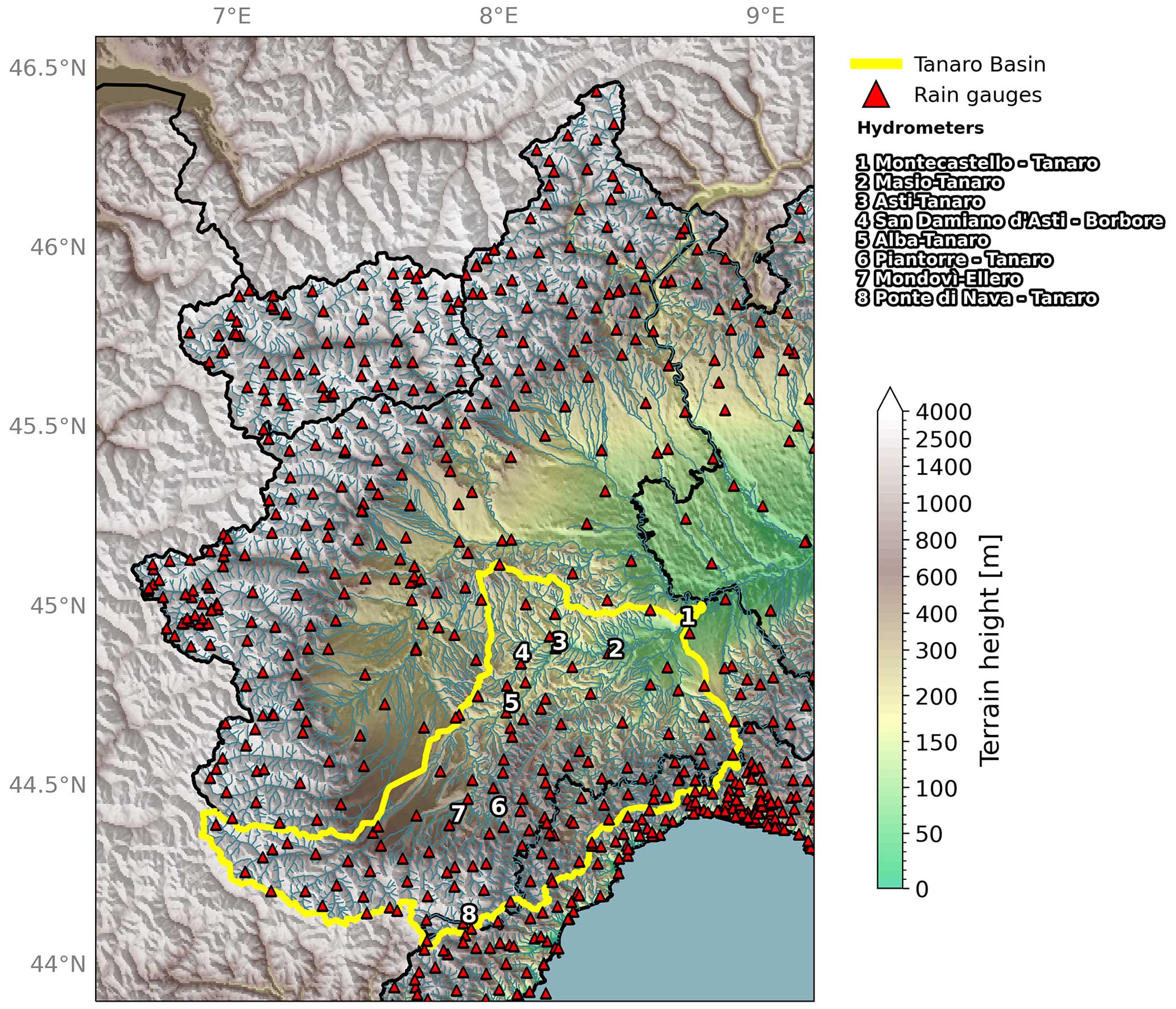
Figure 1 North-west domain of the Italian main drainage network (blue line); the Tanaro River basin is highlighted in yellow. The numbers represent the basin flow discharge stations selected: Montecastello (7956 km² drained), Masio (4535 km² drained), Asti (4123 km² drained), Alba (3385 km² drained), Piantorre (500 km² drained), Mondovì – Ellero (180 km² drained), San Damiano d'Asti – Borbore (85 km² drained) and Ponte di Nava (149 km² drained). The red triangles are the rain gauges available for this study. DEM data are accessible at https://land.copernicus.eu/imagery-in-situ/eu-dem/ (last access: August 2023). The drainage network and boundaries of the basin are accessible at https://www.hydrosheds.org/ (last access: August 2023).

According to Degiorgis et al. (2013), the river is characterized by morphological variability. Three main areas associated with very different characteristics were defined: (1) the mountain zone, with a mean slope of about 6 %, deep riverbeds and very steep catchments; (2) the mild zone, with a mean 1 % slope, mildly steep catchments and shallower riverbeds; and (3) the alluvial zone, with very small slope values.

The Tanaro is the only river among the right-bank tributaries of the Po, and it has an Alpine origin, although the low elevation of the Ligurian Alps and their proximity to the sea do not allow for the formation of snowpack or glaciers large enough to provide a constant source of water during the summer; moreover, the Alpine zone constitutes only part of the basin drained by the Tanaro River. For this reason, under standard seasonal conditions, the flow discharge is subject to great seasonal variations with a regime more typical of an Apennine stream and a maximum flow discharge that can reach 1700 m³ s⁻¹ in spring and autumn and a very low flow rate in summer. The natural flow discharge of the Tanaro River is strongly affected by the anthropic impact due to the fragmentation of the river channels, with dams and water regulation causing diversions between basins and irrigation. Some artificial sections intersect natural branches, and some of these sub-basins are used for hydropower generation. The artificial basins along the river and its tributaries are also used for flood control.

The river is exposed to severe events: it was affected by at least 136 floods in 200 years (from 1801 to 2001). The most significant of these events occurred in November 1994, when the entire river valley was damaged (Marchi et al., 1995; Luino, 2002), and the sensor at Montecastello, located at the outlet of the river, recorded a maximum flow discharge peak of 4350 m³ s⁻¹ (Po River Basin Authority, 2023).

3 Observed data

Precipitation data are recorded for the 2014 period on an hourly basis. The precipitation datasets are discussed below and include the gauge dataset, the satellite-only dataset and the flow discharge data from selected point stations distributed along the Tanaro River basin.

3.1 Rain gauge data

It is common to attribute an area of influence to a network of rain gauges: in detail, the gauge is in the centre of its circular area of influence, defined as the radius of influence; Shi et al. (2020) suggest that the radius of influence, also considered the average distance between stations, can be computed as

$$\begin{array}{}\text{(1)}& R=\sqrt{{\displaystyle \frac{S}{N}}},\end{array}$$

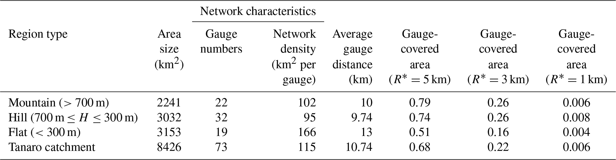
where S is the area of the smallest circle, which can cover all the rain gauges and the considered basin, whereas N is the number of rain gauges considered. Reasonable station coverage means that the average radius associated with the rain gauge network should be at least comparable to the value associated with the rain bandwidth. In this study, S is the area of the Tanaro basin, and N is the number of rain gauges in the basin (73 in the basin): the average distance of the next station is about 11 km, but the stations are not distributed regularly. As will be discussed later, different values of R are selected for the different hydrological simulations. As discussed in Sect. 2, since the Tanaro basin is divided into three territorial sectors, the average rain gauge distance is computed for each of them (see Table 1).

Table 1 Rain gauge network characteristics of the Tanaro catchment; R^* is the Cressman radius of influence.

3.2 Satellite-based rainfall estimates

The satellite precipitation product used in this study is the Global Precipitation Measurement (GPM) Integrated Multi-satellitE Retrievals for GPM (IMERG). The products provide quasi-global (60° N–60° S) precipitation estimates combining measurements from passive microwave (PMW) radiometers comprising the GPM low-Earth-orbit (LEO) satellite constellation and infrared (IR) geostationary (GEO) sensors. The IMERG product is also available in the form of post-real-time research data, i.e. IMERG Final, after monthly rain gauge analysis is received and considered (Huffman et al., 2018; O et al., 2017). Note the IMERG Final product is considered for demonstrative purposes because such a product is not available in near-real time, and therefore it cannot be used in an operational context that requires near-real-time constraints. In this study, IMERG version 5 Final (IMERG-F) uncalibrated (UNCAL) and calibrated (CAL; where the monthly rain gauge data are used for bias correction), half-hourly 0.1°×0.1° (roughly 10 km × 10 km) rainfall rate estimates have been used. It is worth noting that in this study IMERG V05 is used, while a new version (V07) is ready to be issued at the time of the publication of our study. However, the methodological value of the combination approach shown should not be affected by the product version updates, although quantitative checks could merit attention in a future work.

3.3 Observed flow discharge data

Flow discharge data (m³ s⁻¹) are used to evaluate the hydrological model output in response to different precipitation inputs. However, several issues must be considered when the evaluation of deterministic hydrological models is used, including the need to validate them with very long observed flow discharge data time series. These data are not always available, especially for small seasonal streams that are usually not instrumented. Furthermore, data on artificial water management are not available. Hence, the hydrological model validation may encounter difficulties when dealing with heavily regulated basins, as it simulates the natural river flow rate without accounting for artificial facilities. In addition, estimates of river discharge data are associated with significant uncertainties due to various conditions such as rating curve interpolation, extrapolation, unsteady flow condition and seasonal variations in river roughness (Di Baldassarre and Montanari, 2009; Di Baldassarre and Claps, 2011).

Eight stations with long time series of flow discharge, available for the year 2014, are selected for this study. The stations are distributed over the basin, as shown in Fig. 1 (blue numbers), and they are representative of the different sub-basins contained in the Tanaro River basin.

4 Methodology

The workflow methodology is shown in Fig. 2. It includes three main tasks: precipitation gridding and assimilation data, precipitation merging data and hydrological model simulations, and analysis and error score metrics' calculation. Different combinations of precipitation are tested as input to the hydrological model, and error scores are calculated accordingly in terms of flow discharge. The proposed technique for merging different measured rainfall at different spatial scales is based on the concepts of data assimilation (Bouttier and Courtier, 1999) with particular emphasis on the transformation of point data to areal data. Observed satellite and rain gauge data are gridded respecting the resolution set-up of the hydrological model: each value of rain data (satellite or gauge) is associated with a grid point ith of coordinates (l, m) of the selected domain. Different rain scenarios are produced using the original datasets or merged rainfall data; the hydrological model has been forced with different rebuilt hourly rain fields to simulate flow discharges and to evaluate each scenario.

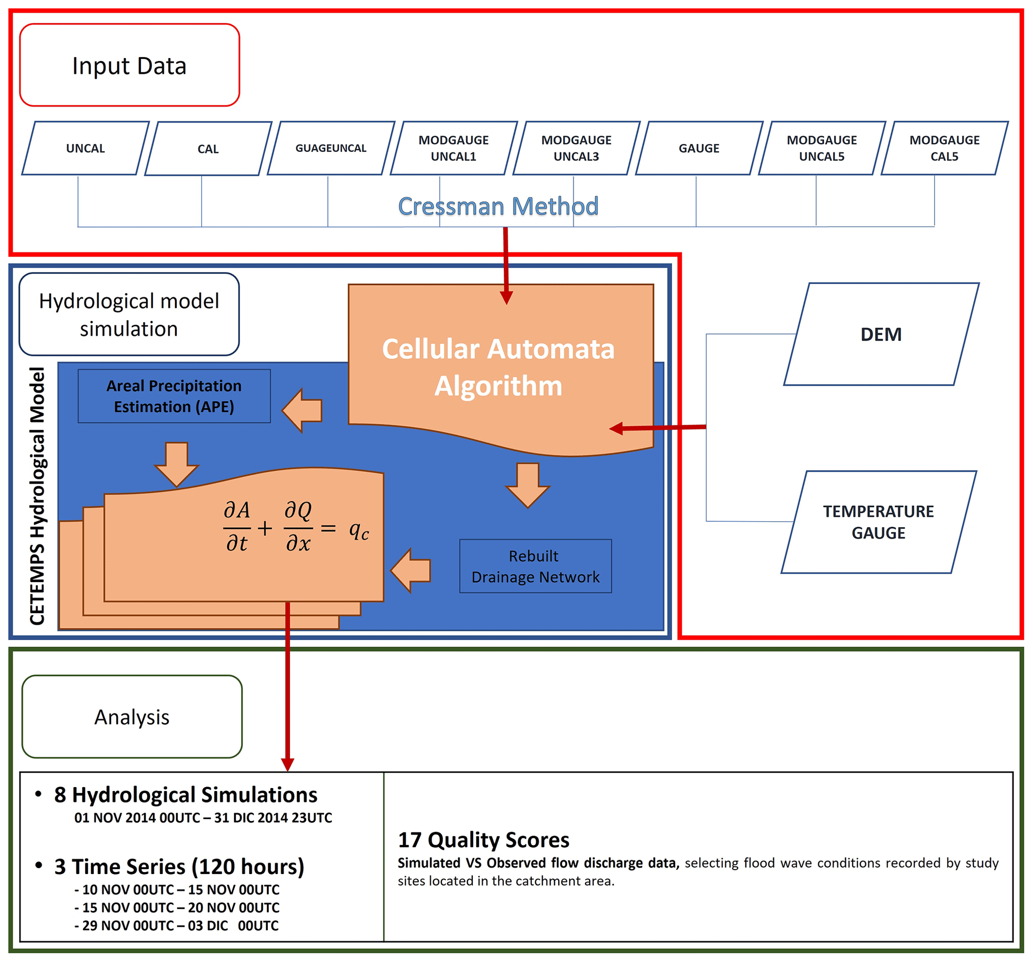
Figure 2 Numerical experiment workflow, consisting of three main tasks: (1) precipitation gridding and assimilation data, (2) precipitation merging data and hydrological model simulations, and (3) analysis and error score calculation. Different combinations of precipitation are tested as input to the hydrological model and error scores calculated accordingly in terms of flow discharge. Eight different simulations have been carried out for each case studies, using the eight different rain input settings.

4.1 Precipitation data gridding

In hydrological modelling, precipitation data gridding is essential to accelerate numerical processing. It involves creating an initial estimate of the precipitation field at the hydrological scale, known as the precipitation background field (PBF; Coppola et al., 2007), on a regular grid. The Cressman algorithm (Cressman, 1959) is commonly used to initialize rain field grid points within the designated domain. Due to its simplicity, the Cressman method serves as a practical starting point for this initialization process (Bouttier and Courtier, 1999).

The accuracy of the merged field significantly depends on the choice of kernel function, as highlighted by Li and Shao (2010). Selecting an appropriate kernel function involves defining a rain radius. The radius of influence, denoted as R, plays a crucial role in determining the smoothness of the estimated field and controlling the spread of the kernel function: a smaller R results in a more rugged estimated field with higher variance, while a larger R yields a smoother surface. Thus, the selection of the radius of influence is critical in determining the overall quality and characteristics of the estimated precipitation field in hydrological modelling applications.

Based on these considerations, given a discontinuous background field, the rainfall for each grid point of the selected domain is estimated as follows:

$$\begin{array}{}\text{(2)}& {\mathit{P}}_i=\sum _j{\displaystyle \frac{\mathrm{1}-{\left({\mathbf{r}}_{ij}/R\right)}^{\mathrm{2}}}{\mathrm{1}+{\left({\mathbf{r}}_{ij}/R\right)}^{\mathrm{2}}}}{\mathit{P}}_j,\end{array}$$

where P_i is the estimated rain value at the ith grid point; P_j denotes the rainfall measurements available within the radius of influence, R; and r_ij is the distance between the rain gauge location j and the grid point i.

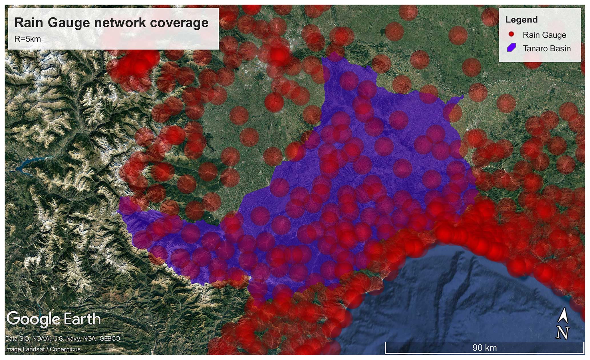
Figure 3 Tanaro basin rain gauge density and distribution. The red circles represents the rain gauge coverage area using a radius of influence of 5 km. The blue line represents the Tanaro basin extent. © Google Earth 2022.

Selecting a suitable value for R poses the initial challenge in the estimation process. Figure 3 illustrates the area coverage by the rain gauge network when employing a radius of influence, R, equal to 5 km. Under the optimal conditions, using observed data available for every grid point in the selected domain without significant errors, employing a direct merging method such as the Cressman objective analysis scheme would still result in considerable bias at the boundary (Li and Shao, 2010; Duque-Gardeazábal et al., 2018). This indicates that while a smaller value of R may mitigate bias, it would only affect a smaller area around the boundary. However, adjusting R does not fully address the issue of boundary bias, as the rain bandwidth tends to be large in cases where observed points are irregularly distributed. The boundary bias issue arises from the discontinuity of the background field due to field discretization, while non-parametric merging methods can only generate continuous surfaces.

To overcome this issue, a double-smoothing merging method is applied. It is used to reduce the boundary bias (Li and Shao, 2010; Duque-Gardeazábal et al., 2018), as better explained in the next section. Furthermore, a strategy used by the work to avoid boundary effects is to extend the spatial domain well beyond the studied basin: this strategy is useful for a better reconstruction of the precipitation field (Fig. 1). Many data used, although redundant, lead to a better reconstruction of the rain field. A smaller amount of data would probably be enough, but the work uses everything that the national rainfall network has available. Future studies could lead to identifying, given their distribution, enough rain gauges outside the basin deemed useful to overcome the boundary effect.

4.2 Precipitation data interpolation and merging: the cellular automata technique

The CA technique is used in this work as a double-smoothing estimation. It is a simple mathematical idealization of natural systems according to Packard and Wolfram (1985), based on the behaviour that every single element of a natural system can assume. In CA, natural systems are idealized as discrete sites on a lattice, with each grid point evolving based on deterministic rules and influenced by the states of neighbouring cells at discrete time steps. This approach provides a structured framework for dynamic systems' modelling, reflecting the intricate interplay of elements in nature.

In the hydrological model code, a CA-based algorithm has been developed and implemented. Following CA theory, the input grid is conceptualized as an aggregate of cellular automata, where the status of each grid point represents the value of a smoothed precipitation field.

The evolution of the precipitation status in the ith grid point of the lattice (${\mathit{P}}_i^{\left(\mathrm{new}\right)}$) is updated according to the following rule:

$$\begin{array}{}\text{(3)}& {\mathit{P}}_i^{\left(\mathrm{new}\right)}={\mathit{P}}_i+\mathit{\alpha }\left(\sum _{i=\mathrm{1}}^{\mathrm{8}}{\mathit{\beta }}_j\left({\mathit{P}}_j-{\mathit{P}}_i\right)\right),\end{array}$$

where ${\mathit{P}}_i^{\left(\mathrm{new}\right)}$ is carried out over all eight surrounding cells. The coefficients β_j allow us to consider the different distances between the cells. As an example, for a regular equally spaced lattice, we assume a value of 1 for the cells in the north, east, south and west locations and a value of $\mathrm{1}/\sqrt{\mathrm{2}}$ for the cells located in the north-east, north-west, south-east and south-west direction with respect to the ith cell.

The coefficient α assumes a small value, typically ranging from 0.1 to 0.9, ensuring a gentle smoothing of the original matrix. All grid points are updated synchronously, and the smoothing continues until stability is achieved, signifying minimal changes in the calculated matrix. Notably, the grid point associated with the rainfall value available in the considered database remains unaltered by the algorithm. This process enables the hydrological model to refine and stabilize the precipitation data while preserving the integrity of observed rainfall values.

Therefore, the rule in Eq. (3) can be written as follows:

$$\begin{array}{}\text{(4)}& P^{t-\mathrm{1}}=P^t+\mathit{\alpha }\sum _{k=\mathrm{1}}^{\mathrm{8}}{\displaystyle \frac{\mathrm{1}}{{\mathit{r}}_k}}{P}_k^t,\end{array}$$

where r_k is the distance between the considered cell and the neighbouring grid point. The value of rainfall in the cells is serially modified (Eq. 4), and the sum is computed using only the neighbouring grid points. The CA method facilitates the assimilation and spatialization of rainfall fields, proving advantageous in achieving the high resolution required in hydrological simulations and in integrating different precipitation data sources.

In this study, to test the assimilation of satellite rainfall data in the presence of sparse gauge stations, the CA algorithm has been implemented in the hydrological model, using two different assimilation approaches: NoModular and Modular. In the NoModular approach, a high-resolution lattice is filled with both the satellite rainfall data and the rain gauge data, used simultaneously at each time step, prioritizing the rain gauge data. To define a PBF, the approach uses an R of 10 km, which corresponds to the satellite spatial resolution, the lowest resolution to cover the whole considered domain; the CA technique is then applied. In the Modular approach, a hierarchical sequence of modules is used to assimilate the different datasets, making it possible to consider the different nature of the data. Therefore, the lattice of the considered domain can be divided into as many subdomains as the data sources' type. Each subdomain can be defined as a set of grid points that have at least one rainfall value in a selected radius, R, whose value depends on the density of the available data. Three different radii of influence were selected in this study to allow for different coverage of rain gauge data compared to the satellite data.

Using the CA technique, this study aims at identifying how different input data settings can affect the hydrological model performance and if merging rain gauge and satellite rainfall data improves hydrological outputs. The degrees of freedom of the input data settings are as follows: (1) the type of data sources – variation in the sources of input data, such as rain gauge data, satellite rainfall data or a combination of both; (2) the data merging approach – comparison between two merging approaches, i.e. (i) NoModular, where rain gauge and satellite data are simultaneously incorporated, prioritizing rain gauge data, and (ii) Modular, which employs a hierarchical sequence of modules to assimilate different datasets independently; (3) the radius of influence, R – exploration of different values for the radius of influence, which determines the coverage area of rain gauge data before applying the CA technique; and (4) satellite data type – evaluation of hydrological model performance using both uncalibrated and calibrated satellite rainfall data. By systematically varying these input data settings, the study aims to provide insights into their respective impacts on the hydrological model's performance. This analysis will contribute to understanding the effectiveness of data assimilation techniques in improving the accuracy and reliability of hydrological simulations.

4.3 Hydrological modelling: CETEMPS Hydrological Model

CHyM has been applied for climatological studies (Coppola et al., 2014; Sangelantoni et al., 2019), but it has mainly been used as an operational tool for early warning systems (Tomassetti et al., 2005; Ferretti et al., 2020; Colaiuda et al., 2020; Lombardi et al., 2021).

CHyM is a distributed, physically based hydrological model; hydrological processes (surface runoff, infiltration, evapotranspiration, percolation, melting and return flow) are explicitly simulated. In addition to being used to acquire different data sources or rebuild the spatial distribution of precipitation at hydrological model scale, the CA algorithm allows the model to simulate the hydrologic cycle of any defined geographic domain and at any fixed spatial resolution up to the digital elevation model (DEM) resolution (90 m in the current version). The choice of spatial resolution is mainly related to the validity of the numerical schemes used to simulate hydrological processes (such as the shallow water kinematic wave used to solve the continuity equation, which is considered a good approximation at a horizontal resolution of a few hundred metres). The hydrological simulation spatial resolution is also related to the different simulated basins: in areas with very small basins close to each other, the resolution must be higher, even up to a few hundred metres; in detail, in this work the spatial resolution used is 900 m. Using CHyM, the spatial domain is extended well beyond the investigated basin. This approach is useful to avoid boundary effects and to have better rebuilding of the precipitation field. Furthermore, CHyM is a valid tool to investigate the rebuilding of the rainfall field, given that the resulting flow discharge value is linked exclusively to the rainfall; in fact the effects related to the base flow discharge are not visible, since the model does not reproduce them, given the short simulation spin-up time. The hydrological model is not specifically calibrated over the Tanaro basin. However, in this work we refer to the calibration accomplished by Coppola at al. (2014) on the northern part of the Po River, which also includes the whole of the Tanaro basin.

4.4 Error score metrics

To assess the fit between the observed and simulated flow discharge time series, objective functions were selected. Traditional performance indicators have been used, such as the Nash–Sutcliffe efficiency (NSE) (Nash and Sutcliffe, 1970) and bias percentage (PBIAS), measuring the average tendency of the simulated values to be larger or smaller than the observed ones. The optimal value of PBIAS is 0.0, with low-magnitude values indicating accurate model simulations. Furthermore, the following scores were considered: root mean square error (RMSE); mean absolute relative error (MARE), which is sensitive to extreme values (i.e. outliers) and to low values; original Kling–Gupta efficiency (KGE; Gupta et al., 2009); modified Kling–Gupta efficiency (KGEprime; Kling et al., 2012); and non-parametric Kling–Gupta efficiency (KGEnp; Pool et al., 2018).

According to Mathevet et al. (2006), KGE and NSE can be calculated in a bounded version: bounded Nash–Sutcliffe efficiency (NSEc2m), bounded original Kling–Gupta efficiency (KGEc2m), bounded non-parametric Kling–Gupta efficiency (KGEmp_c2m) and bounded modified Kling–Gupta efficiency (KGEprime_c2m). The analysis is carried out using an open-source evaluator for flow discharge time series (Hallouin, 2019). In addition to the conventional scores, other indicators were selected to obtain a more objective analysis, independent of the limits of the scores commonly used for hydrological analyses, for a total of 17 quality scores. The idea is to consider the river flow discharge profile as a signal, and for this reason, indicators, commonly used in generic signal studies, have been used.

The match correlation (MC) is the relationship between the auto-correlation curve and the cross-correlation curve (observed vs simulated) and allows us to understand the overlap of the two curves: the best value obtained will be close to 1.

$$\begin{array}{}\text{(5)}& \begin{array}{rl}& \mathrm{MC}=\\ & {\displaystyle \frac{\int \mathrm{AutoCorrelation}\mathrm{\_}\mathrm{of}\mathrm{\_}\mathrm{Observed}\mathrm{\_}\mathrm{values}}{\int \mathrm{CrossCorrelation}\mathrm{\_}\mathrm{of}\mathrm{\_}\mathrm{Index}\mathrm{\_}\mathrm{values}\mathrm{\_}\mathrm{VS}\mathrm{\_}\mathrm{Observed}\mathrm{\_}\mathrm{values}}}\end{array}\end{array}$$

Cross-correlation (CC) is typically used in signal theory for the assessment of similarity between two signals (Rabiner and Gold, 1975; Rabiner and Schafer, 1978; Benesty et al., 2004). The correlation time delay (CT_D, Lombardi et al., 2021) represents an estimation of time shift between two series:

$$\begin{array}{}\text{(6)}& \mathrm{CT}\mathrm{\_}\mathrm{D}=\mathrm{CC}\left(L\right).\end{array}$$

The value of time lag L maximizes the product obtained in the CC calculation. Therefore, this quality score is suitable for measuring the effectiveness of the signal provided by hydrological simulations. The time peak delay (TP_D) is a timing score and represents the hourly delay of the estimated maximum peak flow discharge compared to the observed one.

The percentage error (E%) at the peak value of the flow discharge was calculated as follows:

$$\begin{array}{}\text{(7)}& E={\displaystyle \frac{D_{\mathrm{Sim}}-D_{\mathrm{Obs}}}{D_{\mathrm{Obs}}}},\end{array}$$

where D_sim indicates the simulated flow discharge, and D_Obs represents the observed flow discharge.

Dynamic time warping (DTW; Berndt and Clifford, 1994; Keogh and Ratanamahatana, 2005; Maier-Gerber et al., 2019; Di Muzio et al., 2019) finds the similarity between two sequences by looking for the best alignment. For the N-by-M matrix, built using two discrete series x(i) and y(j) of N and M components, respectively, a “warping” path W is defined as a contiguous set of L matrix elements, and the measure of misalignment d for the path W is given by

$$\begin{array}{}\text{(8)}& d\left(W\right)={\displaystyle \frac{\sum _{i,j}\mathbf{V}(i,j)}{\frac{\mathrm{1}}{\mathrm{2}}L(L-\mathrm{1})}},\end{array}$$

where the sum in the numerator is carried out over all the elements belonging to the warping path W. Each element V(i,j) represents the Euclidean distance between the ith element of the first sequence and jth element of the second sequence.

The denominator is used to normalize different length sequences. The DTW index is then calculated as the minimum value of d(W), considering all the possible paths W.

$$\begin{array}{}\text{(9)}& \mathrm{DTW}=d\left(W\right)\end{array}$$

The optimal path will be the N diagonal elements of matrix V, if the two considered sequences are aligned and have the same number of components (N=M). The DTW technique, however, could lead to wrong results in finding the optimal alignment because a feature (e.g. a local peak or minimum) in one sequence is higher or lower than the corresponding feature in the other sequence. To overcome this issue, Keogh and Pazzani (2001) proposed the computation of warping using the local derivative of the time series to be compared: derivative dynamic time warping (DDTW). The first derivative was calculated for each time series as follows:

$$\begin{array}{}\text{(10)}& D\left(x\right[i\left]\right)={\displaystyle \frac{\left(x\right[i]-x[i-\mathrm{1}\left]\right)+\left(\right(x[i+\mathrm{1}]-x[i-\mathrm{1}])/\mathrm{2}}{\mathrm{2}}}.\end{array}$$

The main limitation linked to both analyses is defined singularities (Sakoe and Chiba, 1978; Keogh and Pazzani, 2001); i.e. the algorithm may try to explain variability in the Y axis by warping the X axis. This can lead to nonintuitive alignments where a single point in one time series maps onto a large subsection of another time series. To overcome these limits, we used the Windowing method (Berndt and Clifford, 1994). Allowable elements of the matrix can be restricted to those that fall into a warping window defined according to the following rule:

$$\begin{array}{}\text{(11)}& \left|i-(n/(m/j\left)\right)\right|<\mathit{\omega },\end{array}$$

where i and j are the allowable points of the n×m matrix, constrained to fall within a given warping window, and ω is a positive integer window width. In this work, ω is equal to 10, and this allows us to mitigate the effects linked to the baseflow discharge.

5 Analysed case studies

One of the effective strategies for the validation of satellite rainfall data is an indirect method through a hydrological assessment. It is worth noting that data on artificial water management are not available for the case study (CS) considered; thus, a preliminary screening is carried out to minimize any anthropogenic impact in our analysis.

In this study, the hydrological simulation ranges from 1 November to 31 December 2014. Since the purpose of this work is to investigate the performance according to the different rain scenarios (model forcing), November and December represent the most suitable period from the climatic point of view: in fact, according to the authors' experience, the succession of rainfall events in the autumn reduces the anthropic impact. In late autumn–early winter, dams and reservoirs are often at the limit of their capacity, allowing the water to laminate, and the river flow discharge is comparable to the natural one, which is simulated by CHyM. Three time series, related to the three different flood events, have been studied:

• Case study 01, 10 November 00:00 UTC–14 November 2014 23:00 UTC;

• Case study 02, 15 November 00:00 UTC–20 November 2014 23:00 UTC;

• Case study 03, 29 November 00:00 UTC–3 December 2014 23:00 UTC.

Figure 4a shows the synoptic charts of the fifth-generation ECMWF reanalysis (ERA5) 500 hPa geopotential height and sea level pressure (Hersbach et al., 2023), related to the first analysed case study (12 November 2014 00:00 UTC). The European scenario was mainly characterized by the presence of a deep depression area located in the North Atlantic and by a persistent blocking system of high pressure in the eastern continental sector. A trough associated with the oceanic depression was slowly moving toward the eastern Mediterranean by rotating its axis. This configuration caused instability conditions in northern Italy, with widespread precipitation, especially in the north-western sectors, and cumulated rainfall of up to 250 mm in 120 h (10 November 00:00 UTC–14 November 23:00 UTC) in the area of interest (Fig. 4d).

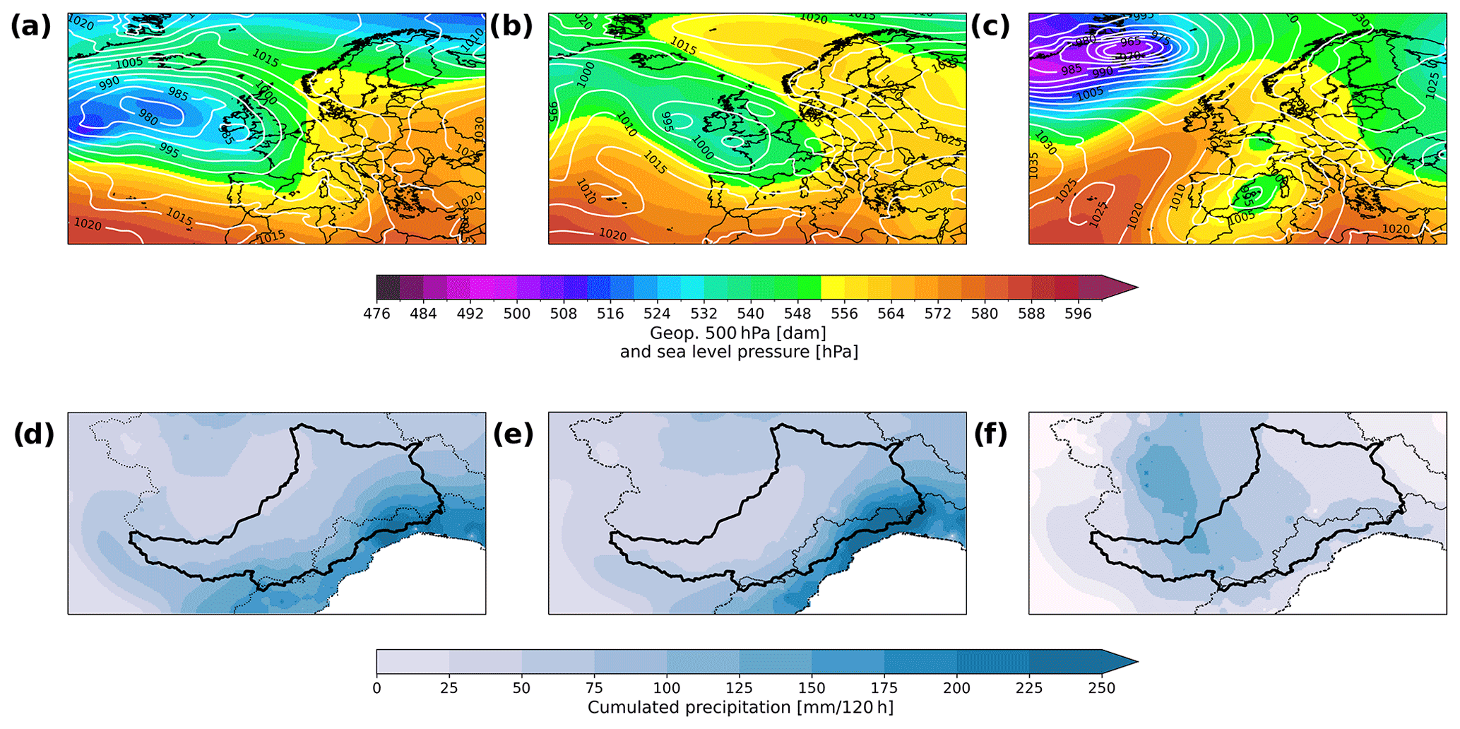
Figure 4 Case studies' synoptic analysis: (a) CS 01 (12 November 2014 00:00 UTC), (b) CS 02 (16 November 2014 00:00 UTC), (c) CS 03 (1 December 2014 00:00 UTC) 500 hPa geopotential height and sea level pressure using the fifth-generation ECMWF reanalysis (ERA5), (d) CS 01, (e) CS 02, and (f) CS 03 120 h cumulated rain rebuilt using rain gauge data.

The synoptic scenario for the second case study (16 November 2014 00:00 UTC) resulted from a slow evolution of that described above. As shown in Fig. 4b, the circulation was slowed down by a high-pressure system located in eastern Europe, extending from Anatolia up to the North Sea, blocking the shift of the Oceanic trough toward the east. The most intense precipitation was recorded in the Italian north-western sectors, with cumulated rainfall up to 250 mm in 120 h (15 November 00:00 UTC–19 November 23:00 UTC) in the area of interest (Fig. 4e).

Figure 4c shows the synoptic situation related to the third case study (1 December 2014 00:00 UTC). In this period, the typical western Mediterranean weather conditions were affected by the evolution of a deep cut-off low. On 29 November, it was centred on Morocco, and in the following days, it moved eastward, advecting subtropical warm and moist air towards north-western Italy. The flux produced intense precipitation in the Ligurian territory, with cumulated rainfall up to 150 mm in 120 h (29 November 00:00 UTC–3 December 23:00 UTC) in the area of interest (Fig. 4d).

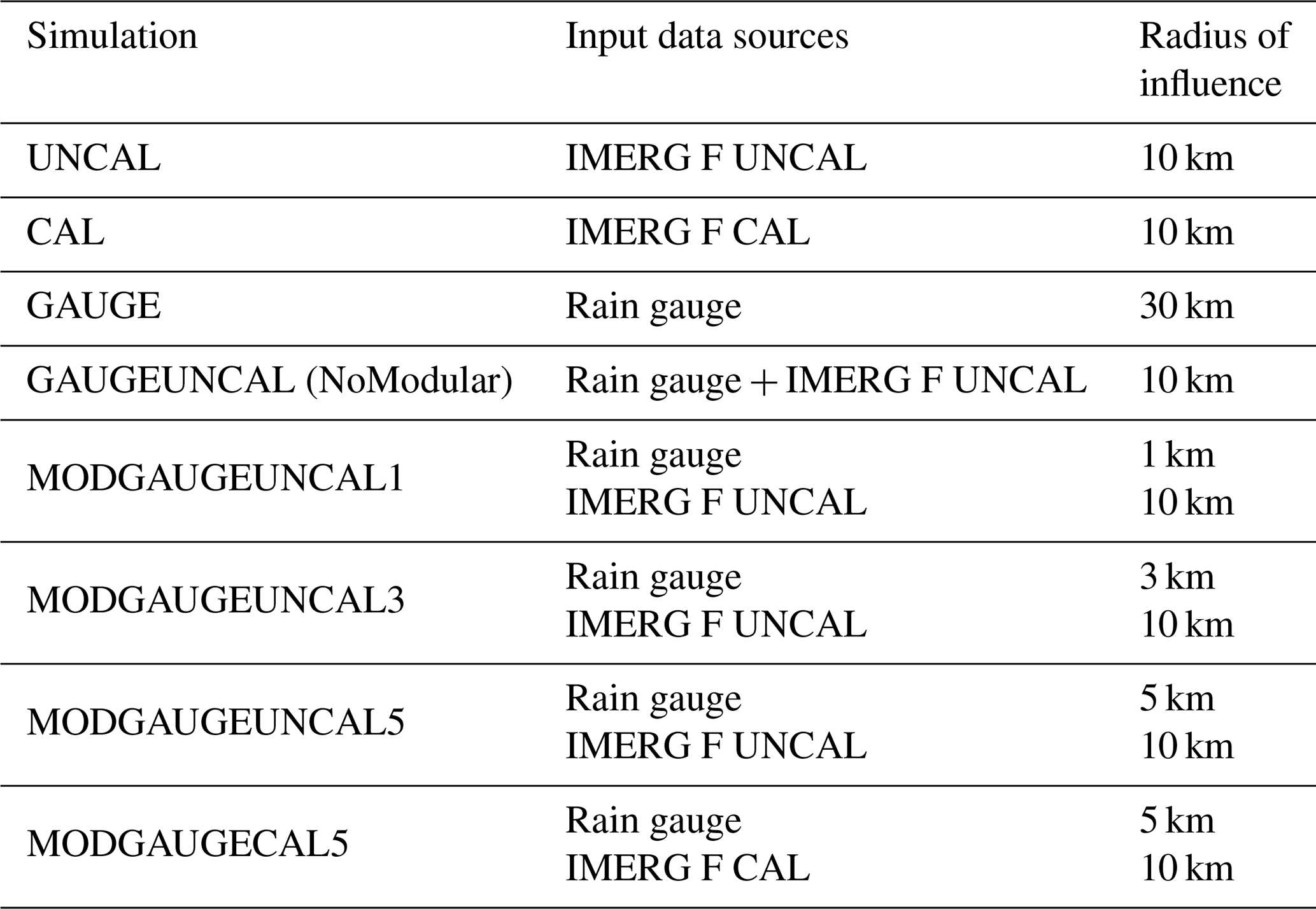
Eight different hourly simulations were carried out for each case study, using the eight different rain input settings (Table 2). Hourly hydrological simulations are possible thanks to the availability of the observed data: the temporal resolution of the hydrological simulations, especially for small hydrological basins that have very short recharge times, is very important, given that satellite data are provided every half hour; they are essential for developing operational monitoring and forecasting tools for flood early warning systems. Therefore, UNCAL and CAL simulations only use satellite data (IMERG-F uncalibrated and IMERG-F calibrated, respectively), while the GAUGE simulation uses the local rain gauge data, and the GAUGEUNCAL simulation uses the combined gauge and satellite data using the NoModular approach. MODGAUGEUNCAL1, MODGAUGEUNCAL3 and MODGAUGEUNCAL5 are the simulations where the hydrological model has been forced using the Modular approach and different radii of influence related to rain gauge data that constitute merged gauge and uncalibrated satellite data (the number at the end of the simulation name is related to the gauge radius of influence: 1, 3 and 5 km), whereas the last hydrological simulation, MODGAUGECAL5, is carried out in the same way but using the calibrated satellite data.

Table 2 Input data sources and settings for each simulation.

6 Results: hydrological simulation analysis

The experiment uses an indirect validation technique of precipitation data, through an analysis of the flow discharge simulated by CHyM, where the model has been forced with eight rainfall scenarios. The APE produced using IMERG F uncalibrated (UNCAL) and calibrated (CAL) and rain gauge data (GAUGE), separately, is based on different R values for each dataset, as defined in Eq. (1). Note that in the case of satellite data, R is fixed to 10 km (the IMERG products' resolution). In the case of GAUGE, R has been set at 30 km, as in the CETEMPS hydrological operational set-up (Colaiuda et al., 2020), to have a coverage of all the points of the grid in the considered domain. Therefore, even if the number of rain gauges that fall in the analysed basin, according to Eq. (1), gives an average distance of the next station of about 11 km, in order to have a total coverage of the entire simulated domain (defined by the coordinates: 43.9 ≤ latitude ≤ 46.59 and 6.49 ≤ longitude ≤ 9.18) and to account for the rain gauge spatial distribution, R cannot be lower than 30 km.

Figure 5 shows the CHyM-rebuilt rain field for Case study 01. In detail, Fig. 5a represents 120 h accumulated rain rebuilt by the GAUGE simulation, obtained by forcing the hydrological model with rain gauge data; Fig. 5b and c, respectively, represent CAL and UNCAL simulations, where CHyM has been forced using GPM IMERG Final CAL and GPM IMERG Final UNCAL, respectively. Figure 5d shows the 120 h cumulated rain related to the MODGAUGEUNCAL5 simulation, obtained by forcing the hydrological model with rain gauge data, using a radius of influence equal to 5 km, merged with GPM IMERG Final UNCAL.

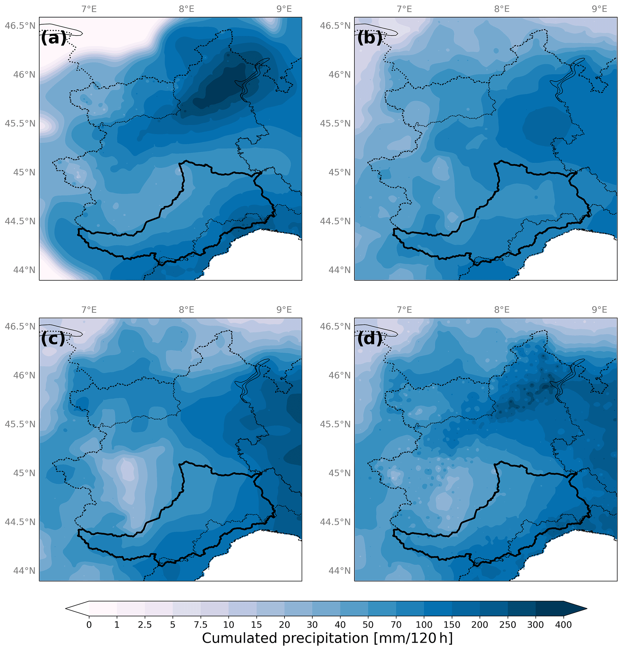
Figure 5 CS 01 areal precipitation estimation: the rain field rebuilt using rain gauge data (a), GPM IMERG Final CAL (b) and GPM IMERG Final UNCAL (c). Panel (d) shows the rain field obtained by forcing the hydrological model with rain gauge data, using a radius of influence equal to 5 km, merged with GPM IMERG Final UNCAL.

The preliminary comparisons related to Case study 01 between observed and simulated flow discharge data with the different rainfall scenarios are shown: in Fig. 6 Alba Tanaro and Ponte di Nava sections were selected for this quick comparison. The hydrometric stations are in sections draining 3385 and 145 km² upstream, respectively. From a first subjective analysis, the model appears to perform better with the GAUGE (cyan line), compared to the use of satellite data only, both UNCAL (grey line) and CAL (yellow line) (Fig. 6a and c), consistently with the literature: rain gauges can be considered the most accurate approach for measurements. A series of sensitivity tests have been carried out, and the most significant are reported (Fig. 6b and d). The tests refer to (i) the approach used, i.e. NoModular or Modular; (ii) the value of R, i.e. 5, 3 and 1 km for the rain gauge data and 10 km for satellite data, respectively; and (iii) the satellite data used, i.e. GPM IMERG Final UNCAL and GPM IMERG Final CAL.

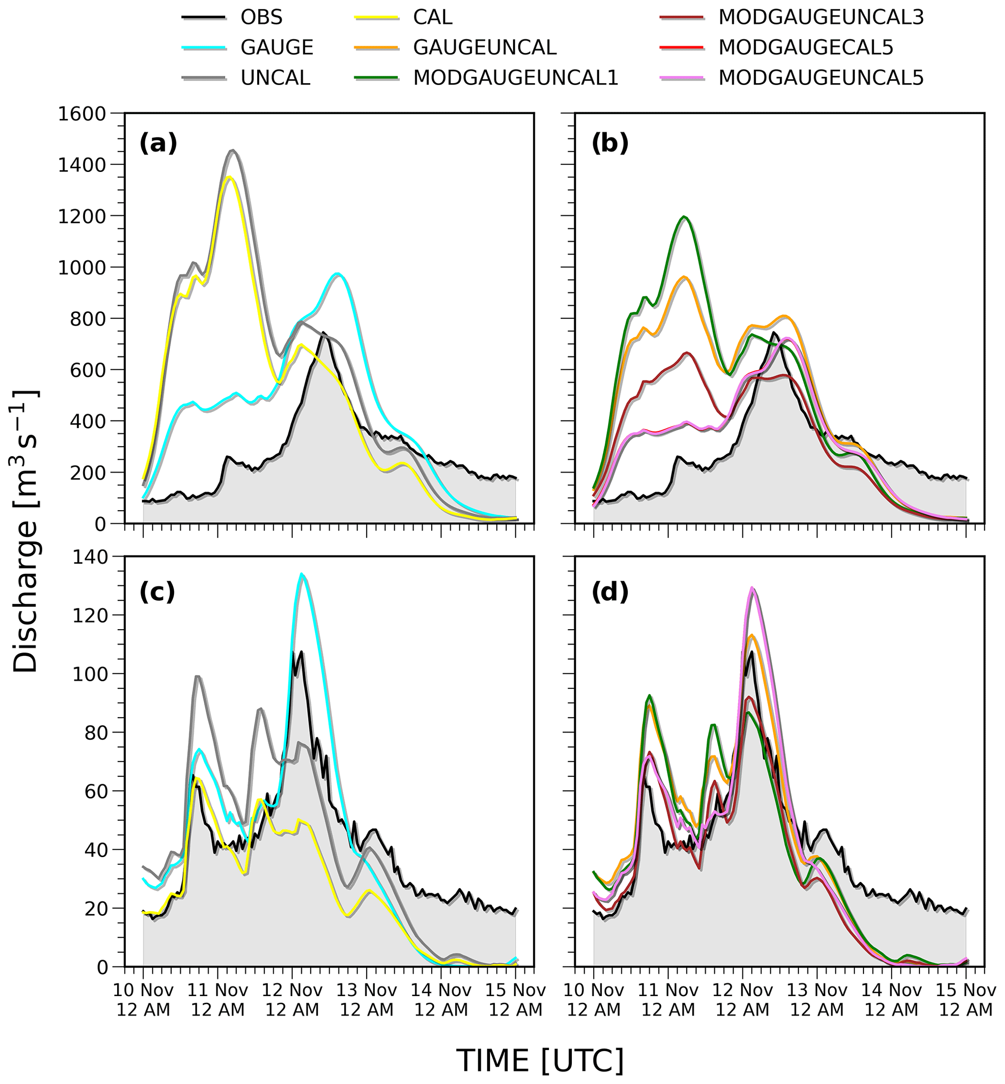
Figure 6 Intercomparison between observed and simulated flow discharge data with the different rainfall scenarios for CS 01. The simulation analysis is related to Alba Tanaro (a, b) and Ponte di Nava (c, d) river sections.

From the analysis of Fig. 6, it can be deduced that the best performances are obtained for MODGAUGECAL5, although comparable performances are obtained using MODGAUGEUNCAL5 (indeed, given the small difference between the two results, the two curves are graphically superimposed). In these cases, the background rain field of the rain gauge data with R=5 km (a coverage of 68 % of the surface of the considered basin, Table 1), smoothed with CA, is merged with the remaining part of the surface covered by the satellite data, where its background areal coverage is first created with R=10 km, filling the grid points left uncovered (32 %) and then applying a definitive smoothing with CA. The scores also confirm the best performances obtained by the simulation using the merged data. As an example, for CS 01 at the Alba section of the river, the KGE assumes values ranging from −1.16 (UNCAL), −0.95 (CAL), −0.703 (MODGAUGEUNCAL1), −0.366 (GAUGEUNCAL) and 0.066 (GAUGE) passing to 0.209 (MODGAUGEUNCAL3) and up to 0.584 (MODGAUGEUNCAL5) and 0.585 (MODGAUGECAL5).

Figure 7 shows the box plots for KGE and RMSE related to all case studies and all river sections and confirms what has been shown so far: certainly, the rain gauge data allow for better performance than using the satellite data alone, but the best results are obtained when the two data sources are merged, especially using the MODGAUGECAL5 setting, which is comparable to MODGAUGEUNCAL5.

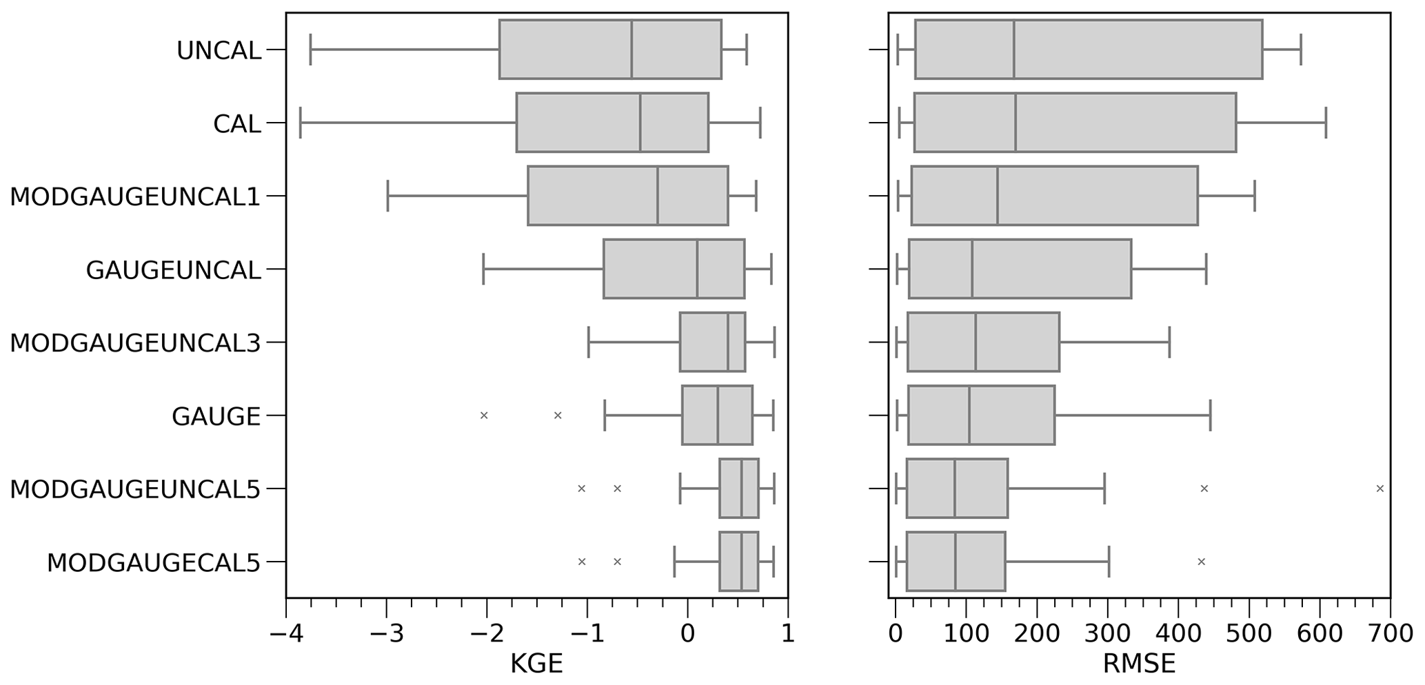
Figure 7 The box plots show the summary of KGE and RMSE obtained from the CHyM simulation using the eight APE fields as input, related to all three case studies and all river sections.

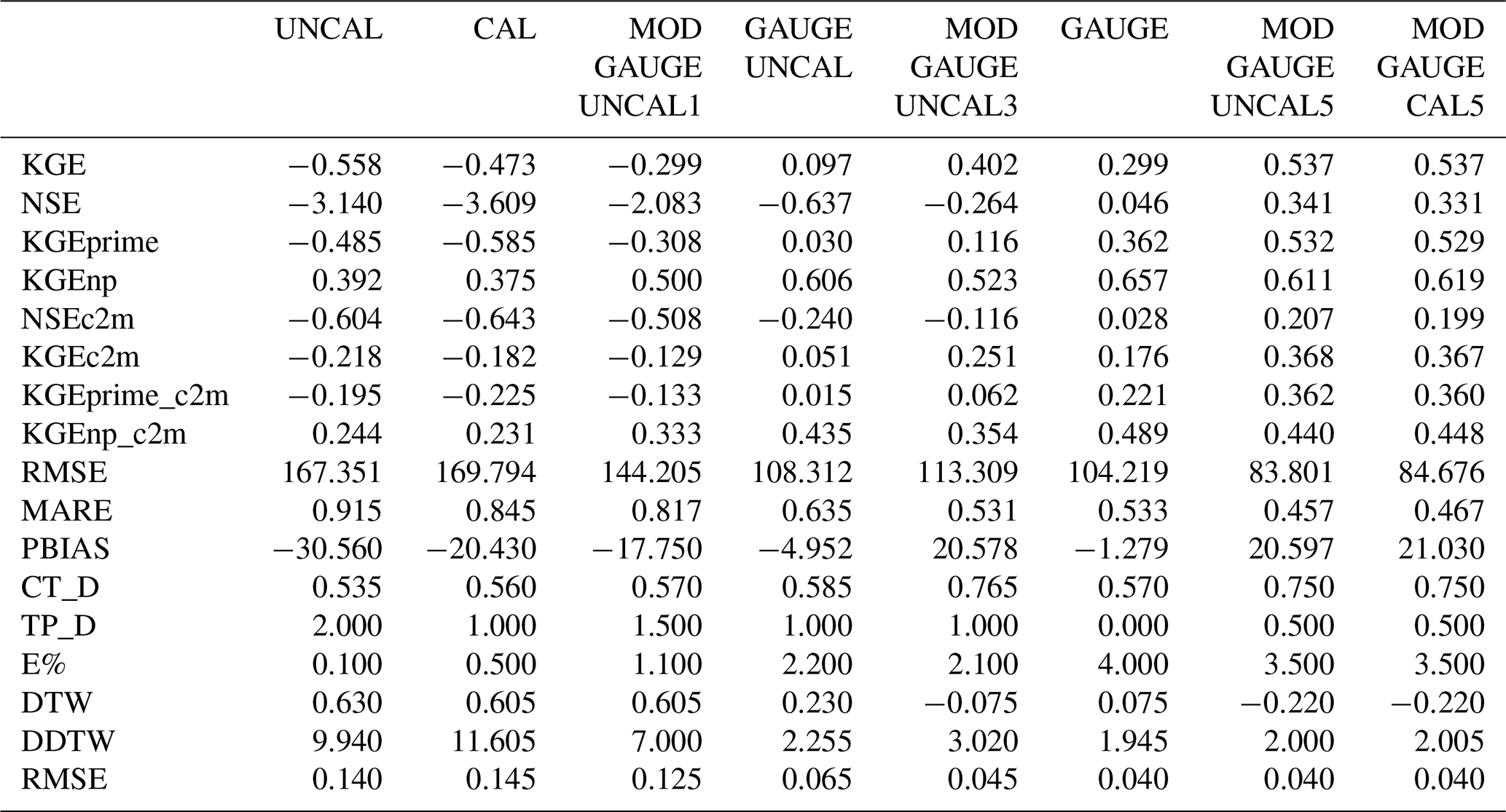
Table 3 Average statistical scores for all three case studies and all river stations obtained from the CHyM simulations using the eight APE fields as input (AVG). The first block of the table shows all the quality scores, where the best performances are identified by a value equal to 1. In the second block of the table, the best performances are identified by values close to zero.

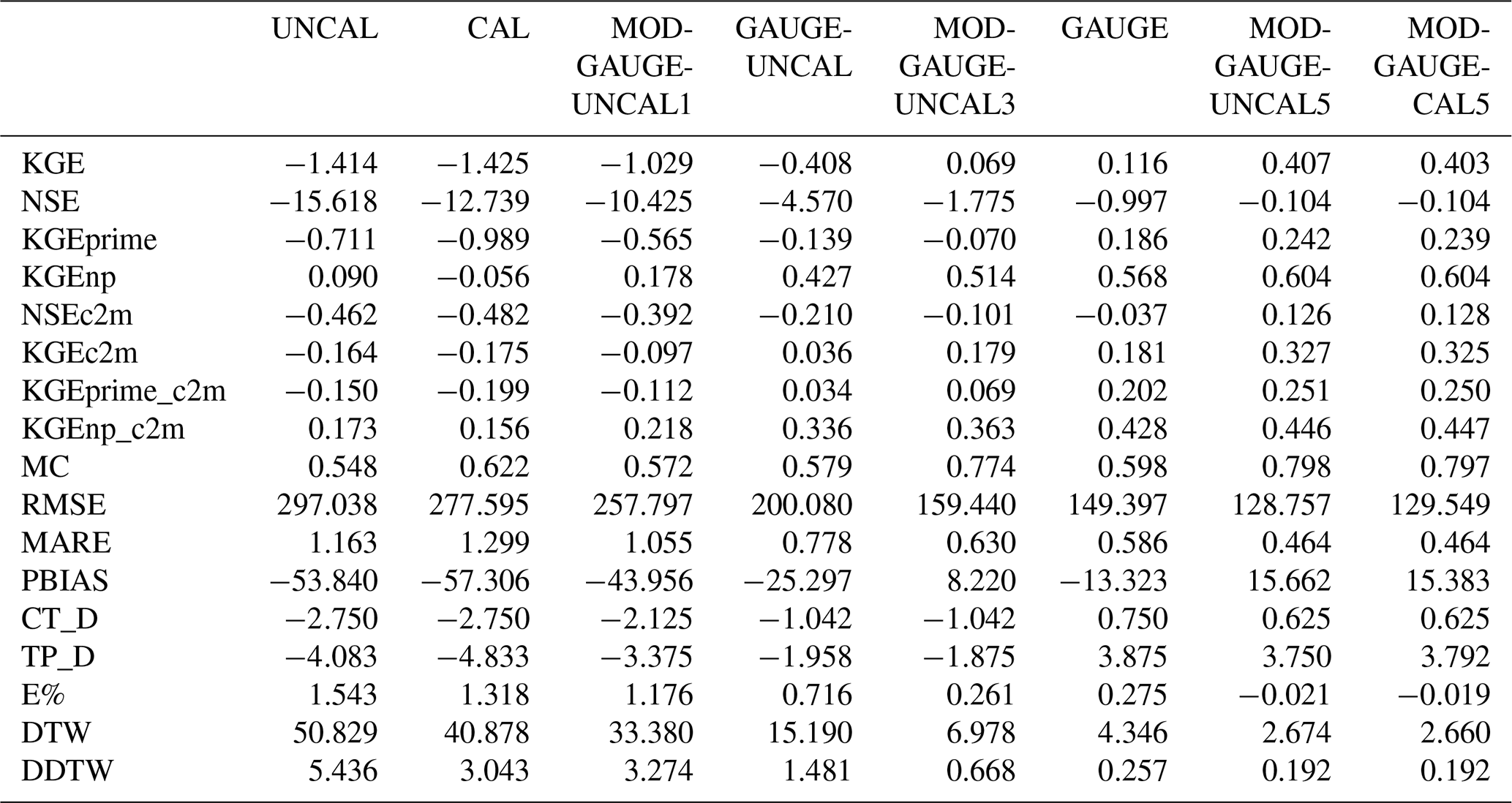
To obtain an objective evaluation, the statistical analysis has been performed using different quality scores, evaluating their overall average (AVG) related to the three case studies and all stations (Table 3). Table 3 is divided into two parts, and the various settings have been placed following the order of increasing performance. In the first part of Table 3, an improvement corresponds to increasing values, while in the second part, an improvement corresponds to decreasing values. All scores confirm the results obtained from the comparison between observed and simulated flow discharges (Fig. 6), showing better performance using the rain gauge data only (GAUGE) compared to satellite data only. Simultaneously, the calibrated satellite data (CAL) allow the model to perform better than the uncalibrated data (UNCAL). There is an evident improvement in the results obtained by merging the different sources of observed data (gauge and satellite) compared to simulations that use only satellite data.

The KGE score, for example, shows the above statement: an AVG ranging from −1.41 for UNCAL to 0.11 for GAUGE to 0.40 for MODGAUGECAL5 (Table 3). MODGAUGEUNCAL3 has comparable performance, although it is less well performing, with respect to GAUGE (only rain gauge data) and to MODGAUGEUNCAL5 and MODGAUGECAL5, where the rain gauge data have a coverage of 68 %. Although they do not improve compared to GAUGE, this is encouraging, suggesting that even with a lower rain gauge density, the performance of the hydrological simulation can be guaranteed. MODGAUGEUNCAL1 has been used to test the minimum bandwidth of rain gauge size in the basin. Not all results are satisfactory; for example, the NSE, a classic skill score in hydrology, is a convenient and popular (albeit gross) indicator of the model's ability (there has been a long and lively discussion about its eligibility; Gupta et al., 2009). The simulation efficiency can be considered significant if the results are greater than 0: if the study results do not respect these conditions, they are negative or at most close to zero. Despite the results, our aim is to verify which APE obtained with the different settings improves the performance of the hydrological model, and the results obtained with the NSE test confirm it: the score goes from −15.618 for the UNCAL simulation (the worst performance) to −0.104 for MODGAUGEUNCAL5 and MODGAUGECAL5 simulations. Figure 8 shows the AVG values, listed in Table 3, of some of the considered scores. In detail, Fig. 8a shows some of the scores where the best performances are identified by a value equal to 1: KGEnp, NSEc2m, KGEc2m and MC.

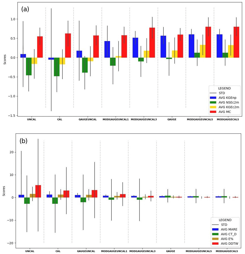
Figure 8 The histograms summarize the statistical analysis performed for the different scores, evaluating their average (AVG) and the standard deviation (SD). Panel (a) shows the quality scores (KGEnp, NSEc2m, KGEc2m and MC), where the best performances are identified by a value equal to 1. In panel (b) (MARE, CT_D, E% and DDTW), the best performances are identified by values close to zero.

In the second part of Table 3, the error is measured in terms of RMSE, MARE and PBIAS. In the case of RMSE and MARE, the trend of the results confirms what has been verified with the other quality scores. Concerning PBIAS, the results are slightly different. The low magnitude of PBIAS indicates an accurate model simulation, where positive values indicate overestimation, and negative values indicate model underestimation. In this case, the best performances are evident for MODGAUGEUNACAL3, GAUGE, MODGAUGEUNCAL5 and MODGAUGECAL5 simulations, although their interpretation is not as straightforward as for other scores. In detail, the overall PBIAS AVG values are 8.22 for MODGAUGEUNACAL3, −13.33 for GAUGE, and about 15 for MODGAUGEUNCAL5 and MODGAUGECAL5 simulations. Also, in this case, as shown in Table 3 and Fig. 8b by CT_D, TP_D, E%, DTW and DDTW, an improvement in performance is confirmed with a clear decrease in the trend.

The comparison between the different Modular settings was necessary to verify if the CA technique could overcome the limit of the satellite rain data calibration. In fact, using a 5 km rain gauge radius of influence, the results are comparable both for calibrated and uncalibrated satellite data.

Table 4 Standard deviation of the statistical scores for all three case studies and all river stations obtained from the CHyM simulations using the eight APE fields as input (SD).

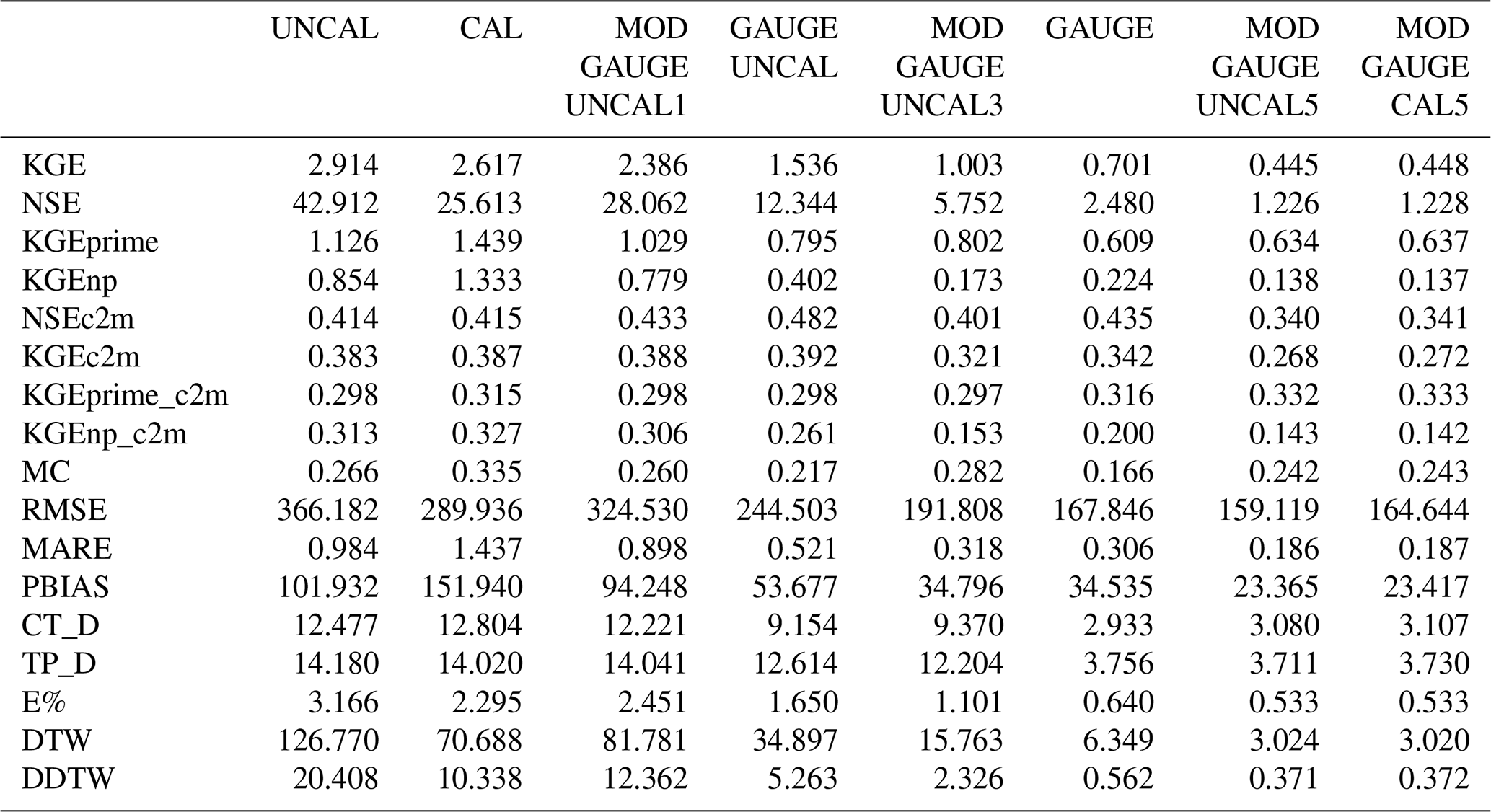
Table 5 Median of the statistical scores for all three case studies and all river stations obtained from the CHyM simulations using the eight APE fields as input (MED).

Regardless of the setting of the different runs, an improvement in results is obtained by merging rain gauges and uncalibrated satellite data compared to using only calibrated GPM IMERG; an improvement was also found by merging the data compared with using only rain gauge data. Thus, the Modular approach with R=1 km (MODGAUGEUNCAL1) provides a less-well-performing hydrological simulation than the NoModular approach (GAUGEUNCAL), while a strong performance improvement is evident with the Modular approach, where rain gauges have R=5 km (MODGAUGEUNCAL5 and MODGAUGECAL5), compared with the simulation using only rain gauge data (GAUGE). All the other scores reflect the expected trend: the performance of the model improves by merging the data, but above all, using this approach, whether calibrated or uncalibrated satellite data are used, the performances are comparable. In addition to using the average values (AVG) of the scores, the overall median (MED) and the overall standard deviation (SD) for the different runs have been computed, and they are reported in Tables 4 and 5. A general increase in performance using merged data is also obtained for MED and for SD.

7 Conclusions

Hydrological models are crucial aids for flood early warning systems and water resource management, particularly in the context of climate change. The accuracy of the results of many hydrological calculations depends on the accuracy of the areal precipitation estimation (APE): a more realistic rainfall distribution is as important as the correct estimation of the cumulative rainfall maxima, especially when severe weather events affect areas with a complex drainage network and characterized by small- to medium-sized river basins in close proximity to each other. Accurate estimation of the APE using rain gauge measurement interpolation is widely used, although the use of radar and satellite data is increasingly common. To correct spatial errors caused by variability in precipitation over short distances, different data sources are necessary. As these errors are linked to the density and distribution of rain gauges, they impact the streamflow simulation model's performance. In fact, the arrangement of rain gauges in the monitoring network may not meet the minimum density standard set by the WMO, as in the selected domain, particularly in areas with diverse topography. Consequently, the use of modern remote sensing techniques, including radar or satellite data, is indispensable in regions with scarce or non-existent rain gauges.

The study highlights the benefit of using satellite-based rainfall estimation precipitation products for hydrological simulations, especially in those areas where there is no homogeneous distribution of rain gauges, and it is a detailed analysis of the potential usage of the cellular-automata-based algorithm developed and implemented in the CHyM code to merge different rainfall data inputs.

This work supports the relevance of using different data sources simultaneously as well as providing methodologies for dealing with them (rain gauges and satellite rainfall estimates): different data sources are used to obtain a mutual correction of the implicit error typical of different sources. An important aspect is choosing the right methodology for using the data. The main aim of this work is to validate the CA technique as a tool for creating the APE using rain gauge and satellite rainfall data. The temporal resolution of these data sources (rain gauge is provided every hour instead of satellite data every half hour) is essential for developing operational monitoring and forecasting tools for flood early warning systems.

Eight different simulations have been carried out, where the hydrological model has been forced with different CA-based APE scenarios.

For the comparison between observed and simulated flow discharge time series, objective functions were selected. Traditional performance indicators have been used: KGE, NSE and the bounded version (KGEprime, KGEnp, NSEc2m, KGEc2m, KGEprime_c2m, KGEnp_c2m). RMSE, MARE and PBIAS were also considered. In addition, typical signal theory indicators (MC, CT_D, TP_D, E%, DTW and DDTW) were selected to obtain a more objective analysis, independent of the limits of the scores commonly used for hydrological analyses.

Three different case studies have been selected, and the statistical analysis has been performed using different quality scores, evaluating their overall average related to the three case studies and all station time series. The results show an improvement in the performance of hydrological simulations when satellite and rain gauge data are merged. In detail, all scores confirm better performance using only rain gauge data (GAUGE) compared to satellite data (UNCAL, CAL), with results ranging from negative KGE values, −1.414 and −1.425, respectively, for the UNCAL and CAL simulations (as reported in Table 3), to the value 0.116 of the GAUGE simulation. Considering that in the case of the KGE score the best performances are identified by values close to 1, the best performances are associated with the model outputs forced with the APE obtained by starting from a rain gauge background rain field characterized by radius of influence of R=5 km (i.e. when 68 % coverage of the Tanaro basin is associated with the rainfall estimated through the gauge data), and the remaining part of the area is covered by the rainfall field rebuilt using the GPM IMERG product (calibrated or uncalibrated), which has a KGE value of approximately 0.4. Less-well-performing results than the GAUGE simulation are obtained with the other settings. Obviously, the objective of this work is not to verify the perfect performance of the hydrological model but to demonstrate how different rainfall fields can improve hydrological simulations.

The same performances are confirmed if the typical signal theory indicators are used, where the best performances are identified by values close to zero: DDTW takes values ranging from 5.43 to 3.043 for UNCAL and CAL, respectively, to 0.257 for the GAUGE simulation. Also, in this case the MODGAUGEUNCAL5 and MODGAUGECAL5 simulations are comparable to each other, with a value of 0.192, and perform better than the other simulations. Regarding the timing indices, CT_D and TP_D, the results are comparable in all simulations. Only a few hours of shifting compared to the observed data makes the performances reliable for all simulations, regardless of the rainfall field. In any case, the CT_P confirms the best performances for the MODGAUGEUNCAL5 and MODGAUGECAL5 simulations with a score value of 0.625 compared to the worst results obtained with the UNCAL and CAL simulations with a score value of −2.75. The results for TP_D are different, where the best performances are obtained with the MODGAUGEUNCAL3 simulation, with an average advance of the maximum peak of approximately 2 h compared to the observed data. The same result is also obtained for the PBIAS score, measuring the average tendency of the simulated values to be larger or smaller than the observed ones, where the best average performances are obtained in the MODGAUGEUNCAL3 simulation.

In the future, this method will be tested on a larger number of case studies and different river basins, as well as on other satellite products (available at different spatial and temporal resolution and shorter latency) to investigate the advantage of the proposed approach in an operational setting for near-real-time hydrological applications.