On the importance of plant phenology in the evaporative process of a semi-arid woodland: could it be why satellite-based evaporation estimates in the miombo differ?

The miombo woodland is the largest dry woodland formation in sub-Saharan Africa, covering an estimated area of 2.7–3.6 million km². Compared to other global ecosystems, the miombo woodland demonstrates unique interactions between plant phenology and climate. For instance, it experiences an increase in the leaf area index (LAI) during the dry season. However, due to limited surface exchange observations in the miombo region, there is a lack of information regarding the effect of these properties on miombo woodland evaporation. It is crucial to have a better understanding of miombo evaporation for accurate hydrological and climate modelling in this region. Currently, the only available regional evaporation estimates are based on satellite data. However, the accuracy of these estimates is questionable due to the scarcity of field estimates with which to compare. Therefore, this study aims to compare the temporal dynamics and magnitudes of six satellite-based evaporation estimates – the Topography-driven Flux Exchange (FLEX-Topo) model, Global Land Evaporation Amsterdam Model (GLEAM), Moderate-Resolution Imaging Spectrometer (MODIS) MOD16 product, operational Simplified Surface Energy Balance (SSEBop) model, Thornthwaite–Mather climatic Water Balance (TerraClimate) dataset, and Water Productivity through Open access of Remotely sensed derived data (WaPOR) – during different phenophases in the miombo woodland of the Luangwa Basin, a representative river basin in southern Africa. The goal of this comparison is to determine if the temporal dynamics and magnitudes of the satellite-based evaporation estimates align with the documented feedback between miombo woodland and climate. In the absence of basin-scale field observations, actual evaporation estimates based on the multi-annual water balance (E_wb) are used for comparison. The results show significant discrepancies among the satellite-based evaporation estimates during the dormant and green-up and mid-green-up phenophases. These phenophases involve substantial changes in miombo species' canopy phenology, including the co-occurrence of leaf fall and leaf flush, as well as access to deeper moisture stocks to support leaf flush in preparation for the rainy season. The satellite-based evaporation estimates show the highest agreement during the senescence phenophase, which corresponds to the period of high temperature, high soil moisture, high leaf chlorophyll content, and highest LAI (i.e. late rainy season into the cool-dry season). In comparison to basin-scale actual evaporation, all six satellite-based evaporation estimates appear to underestimate evaporation. Satellite-based evaporation estimates do not accurately represent evaporation in this data-sparse region, which has a phenology and seasonality that significantly differ from the typical case in data-rich ground-truth locations. This may also be true for other locations with limited data coverage. Based on this study, it is crucial to conduct field-based observations of evaporation during different miombo species phenophases to improve satellite-based evaporation estimates in miombo woodlands.

1 Introduction

Vegetation phenology refers to the periodic biological life cycle events of plants, such as leaf flushing, senescence, and corresponding temporal changes in vegetation canopy cover (Stckli et al., 2011; Cleland et al., 2007). Plant phenology and climate are highly correlated (Pereira et al., 2022; Schwartz, 2013; Cleland et al., 2007). Plants respond to triggers, such as temperature, hydrology and daylight, by initiating, among others: leaf fall, leaf flush, budburst, flowering, and variation in photosynthetic activity (Pereira et al., 2022; Schwartz, 2013; Cleland et al., 2007). Phenological responses are species-dependent and are controlled by adapted physiological properties (Lu et al., 2006). Plant phenology controls the access to critical soil resources, such as nutrients and water (Nord and Lynch, 2009). Moreover, phenological response influences plant canopy cover and affects interactions between phenology and climate. Spatial and temporal variations in canopy leaf display, e.g. due to leaf fall and leaf flush, influence how much radiation is intercepted by plants (Shahidan et al., 2007). Intercepted radiation has shown to influence plant transpiration (Auzmendi et al., 2011; Pieruschka et al., 2010). In water-limited conditions, at both individual species and woodland scales, leaf fall reduces canopy radiation interception, while leaf flush and the consequent increase in canopy cover increase canopy radiation interception, leading to increased transpiration (Snyder and Spano, 2013) controlled by moisture availability, be it in the vegetation itself or in the root zone (Tian et al., 2018). Plant canopy cover and its interactions with atmospheric carbon dioxide influence transpiration (Marchesini et al., 2015). Ultimately, plant phenological response to changes in the triggers influences transpiration and actual evaporation of the woodland (i.e. Marchesini et al., 2015). Miralles et al. (2020) defined evaporation as “the phenomenon by which a substance is converted from its liquid into its vapour phase, independently of where it lies in nature”. In this study, we adopt the term evaporation for all forms of terrestrial evaporation, including transpiration by leaves, evaporation from intercepted rainfall by vegetation and woodland floor, soil evaporation, and evaporation from stagnant open water and pools (Savenije, 2004). Evaporation of woodland surfaces accounts for a significant portion of the water cycle on the terrestrial landmass (Sheil, 2018; Van Der Ent et al., 2014, 2010; Gerrits, 2010). Understanding the characteristics of evaporation, such as interception and transpiration, in various woodland ecosystems is key to monitoring the climate impact on woodland ecosystems and for hydrological modelling and the management of water resources at various scales (Kleine et al., 2021; Bonnesoeur et al., 2019; Roberts, 2013). Knowledge of the woodland phenology interactions with climate variables and seasonal environmental regimes is key to this understanding (Zhao et al., 2013). Environmental variables, such as precipitation and temperature, influence plant phenology differently across the diverse ecosystems globally (Kramer et al., 2000; Forrest et al., 2010; Forrest and Miller-Rushing, 2010). Additionally, Tian et al. (2018) showed that, at the ecosystem scale, plants have adapted to local climatic (such as precipitation, temperature, and radiation) and abiotic (such as soil type and soil water supply) conditions. The findings by Tian et al. (2018) are “evidence of global differences in the interaction between plant water storage and leaf phenology”. Although this study referred to within-plant storage of moisture, it may be as relevant to root zone storage or access to groundwater. Therefore, understanding the interactions between plant phenology and climate at local and regional scales and appropriately incorporating these aspects in hydrological and climate modelling is likely to improve the accuracy of the simulations (Forster et al., 2022).

The miombo woodland is the largest dry woodland formation in sub-Saharan Africa, with a spatial extent of approximately between 2.7 and 3.6 million km², covering about 10 % of the continent (Ryan et al., 2016; Guan et al., 2014; White, 1983). Despite their significance for biodiversity (Mittermeier et al., 2003; White, 1983); carbon sink (Pelletier et al., 2018); and food, energy, and water nexus (Beilfuss, 2012; Campbell et al., 1996; Frost, 1996), little attention has been paid to its hydrological functioning. The uniqueness of the interactions between plant phenology and climate in the miombo woodland has been highlighted (Tian et al., 2018; White 1983) and has been particularly demonstrated by Tian et al. (2018), Vinya et al. (2018), Fuller (1999), Frost (1996), and White (1983). Of particular importance is its control of leaf phenology (i.e. Vinya et al., 2018), co-occurring of leaf fall (leaf shedding) and leaf flush (i.e. Fuller, 1999), and deep rooting, which allows miombo species to access deep soil moisture, including groundwater, to buffer for dry-season water limitations (Tian et al., 2018; Guan et al., 2014; Savory, 1963). Most remarkably, new leaf flushing occurs before the commencement of seasonal rainfall (Chidumayo, 1994; Fuller and Prince, 1996). Young flushed leaves in the dry season have a high water content of up to 66 %, which declines to about 51 % as the leaves harden until they are shed off in the next season (Ernst and Walker, 1973). The miombo woodland is heterogeneous with species diversity, whose phenological response to stimuli is species-dependent (Frost, 1996). For instance, leaf fall, leaf flush, and leaf colour change are triggered at different times for each species. This means that the miombo woodland is unlike other woodlands where leaf fall and leaf flush occur in different seasons. In the Miombo, the co-occurrence of leaf fall and leaf flush results in a woodland canopy that is variable in terms of canopy closure and greenness, especially during the dry season. As a result, it has varied canopy closure ranging from 2 % to about 70 %, depending on the miombo woodland strata and local environmental conditions such as rainfall, soil type, soil moisture, species composition, and temperature (Frost, 1996). The wet miombo woodland receives a mean annual rainfall of above 1100 mm, while the dry miombo woodland receives a mean annual rainfall of less than 1100 mm (Fuller and Prince, 1996; Chidumayo, 1987; White, 1983). The depth to groundwater ranges between 0 and 25 m b.g.l. for both wet miombo woodland and dry miombo woodland, although, in a few places, the range is between 25 and 50 m b.g.l. (Bonsor and Macdonald, 2011). For the wet miombo woodland with a canopy closure of about 70 %, at any given time, there is a relatively large woodland canopy surface for radiation interception. The deep rooting in most miombo species (Savory, 1963) potentially provides access to deep soil moisture resources like those observed in ecosystems globally (Fan et al., 2017; Kleidon and Heimann, 1998). It appears that in the miombo woodland, soil moisture increases with depth (Chidumayo, 1994; Jeffers and Boaler, 1966; Savory, 1963). As a result, the canopy provides an evaporative surface that in combination with other environmental variables, possibly facilitates continued transpiration even during the driest periods (Liu et al., 2022; Jia and Wang, 2021). Most miombo species are broad-leaved, with the capacity for radiation interception (Fuller, 1999) and rainfall interception of up to 20 % in wet miombo woodland (Alexandre, 1997). These typical phenological and physiological attributes are of particular importance for evaporative processes (Forster et al., 2022; Snyder and Spano, 2013; Schwartz, 2013).

Regardless of the uniqueness and importance of the miombo woodland, there exists scant, if any, information on its evaporation dynamics. Most studies on the miombo woodland concentrated on the characterisation of woodland plant species (e.g. Chidumayo and Gumbo, 2010; Chidumayo, 2001; Fuller, 1999; Frost, 1996), its role as a carbon sink (Pelletier et al., 2018), and the social–economic relevance of the ecosystem (Frost, 1996). There is ample information on the phenology of plant species (e.g. Chidumayo and Gumbo, 2010; Chidumayo, 2001; Fuller, 1999; Frost, 1996), but there have been very limited attempts to characterise evaporation of the miombo ecosystem, especially during the dry season. Based on the literature in the public domain, Zimba et al. (2023) is the only point-based field observation of evaporation in the miombo woodland. They found that all the satellite-based estimates they compared to field observations underestimated dry-season and early-rainy-season actual evaporation in the wet miombo woodland. Furthermore, they showed that in the dry season (June–October), except for WaPOR, the temporal dynamics of the satellite-based estimates differed from that of the field observations. These point-based estimates by Zimba et al. (2023) are not sufficient to make any definitive conclusions about the evaporative dynamics of this vast ecosystem. The study was limited in both time and space: it did not cover all the phenophases of the miombo woodland; it was only conducted in the wet miombo woodland and was limited to the point location in Mpika, Zambia. For a more expanded understanding of the evaporation dynamics of the miombo woodland, there is a need for the comparison of satellite-based estimations across all the phenophases, covering both the dry season and the wet season in both dry miombo woodland and wet miombo woodland.

In the absence of spatially distributed field observations, satellite-based evaporation estimates are valuable alternatives, though they come with their own limitations (Zhang et al., 2016). It is well established that evaporation depends on land cover (Han et al., 2019; Liu and Hu, 2019; Wang et al., 2012), but, because of the differences in algorithms, processes, and inputs, satellite-based evaporation estimates differ for the same land surface (Cheng et al., 2021; Zhang et al., 2016). Currently, satellite-based evaporation estimates at various scales are available – e.g. the Global Land Evaporation Amsterdam Model (GLEAM) (Martens et al., 2017; Miralles et al., 2011), Moderate-resolution imaging spectrometer (MODIS) MOD16 product (Running et al., 2019; Mu et al., 2011, 2007), operational Simplified Surface Energy Balance (SSEBop) model (Senay et al., 2013), and Water Productivity through Open access of Remotely sensed derived data (WaPOR) (FAO, 2020). The classification of the various satellite-based evaporation estimates has been extensively discussed by Zhang et al. (2016) and Jiménez et al. (2011, 2009). Most of these satellite-based evaporation estimates were primarily developed for agricultural crops (i.e. Biggs et al., 2015). Additionally, satellite-based evaporation estimates perform differently depending on the land surface (Cheng et al., 2021; Zhang et al., 2016). However, natural woodlands have different interactions between plant phenology and climate and evaporation characteristics (Wang-Erlandsson et al., 2016; Snyder and Spano, 2013; Schwartz, 2013). There is currently no publication in the public domain that shows how various satellite-based evaporation estimates compare in the miombo woodland and especially none with a focus on the unique interactions between phenology and hydrology in miombo species across different phenophases and seasons. Yet, the use of satellite-based evaporation estimates in hydrological modelling, climate modelling, and management of water resources, globally and in Africa, is increasing (i.e. García et al., 2016; Zhang et al., 2016; Makapela, 2015). However, because of the absence or scarcity of field observations and extremely limited validation, it is impossible to know which satellite-based evaporation estimates are close to the actual conditions of the miombo woodland. If any, the choice for a satellite-based evaporation product is based on validation results in non-miombo woodlands or at a scale that includes other woodland types (i.e. Weerasinghe et al., 2020). For instance, an evaporation estimation approach that performs well in energy-limited conditions or homogeneous woodlands (i.e. Bogawski and Bednorz, 2014) cannot be assumed to have the same performance in a warm, water-limiting, and heterogeneous woodland such as the miombo. Therefore, there is a need to validate evaporation products at the local and regional levels in order to improve the outcomes in the use of satellite-based evaporation products. Although Weerasinghe et al. (2020) compared satellite-based evaporation estimates in the Zambezi Basin, whose vegetation cover, among many others, comprises the miombo woodland, the focus of their study was not on the miombo woodland. Furthermore, Weerasinghe et al. (2020) did not attempt to link the differences in the satellite-based evaporation estimates with the phenology of the miombo woodland. The results they observed at the Zambezi Basin scale might be different at a sub-basin level, such as that of the Luangwa Basin.

This study addresses the performance of satellite-based evaporation estimates during different phenophases of the miombo woodland with a focus on the Luangwa sub-basin of the Zambezi, one of the largest river basins in the miombo ecosystem. The Luangwa basin contains both dry (i.e. Southern miombo woodlands) and wet (i.e. Central Zambezian miombo woodlands) miombo. The Central Zambezian miombo woodland is the largest of the four miombo woodland sub-groups, the other three being the Angolan miombo woodland, the Eastern miombo woodland, and the Southern miombo woodland (Frost, 1996; White, 1983). The Luangwa Basin is largely covered by miombo woodland, with the mopane woodland occupying a much smaller area of the basin (Frost, 1996; White, 1983). These attributes suggest a catchment that provides a fair representation of miombo woodlands and an appropriate site for studying its evaporation characteristics.

Hence, the aim of this study is twofold:

• to compare the temporal dynamics and magnitudes of six freely available satellite-based evaporation estimates across different phenophases of the miombo woodland and

• to compare satellite-based evaporation estimates to the water-balance-based actual evaporation estimates for the Luangwa Basin.

2 Materials and methods

2.1 Study site

The location and extent of the miombo woodland in Africa is presented in Fig. 1a (Ryan et al., 2016; White, 1983). The Luangwa (Fig. 1) is a sub-basin of the Zambezi Basin in sub-Saharan Africa in Zambia, with a spatial extent of about 159 000 km² (Beilfuss, 2012; World Bank, 2010). Based on the miombo woodland delineation by White (1983) and Ryan et al. (2016), as given in Fig. 1b, about 75 % of the total Luangwa Basin landmass is covered by the miombo woodland, both dry and wet miombo. Additionally, statistics from the 2019 Copernicus Land Cover classification (Fig. S1 in the Supplement) indicate that 77 % of the total basin area is woodland (dense and open woodland), which is largely miombo woodland, with a smaller component of mopane woodland in the middle area of the basin (Buchhorn et al., 2020a, b; Martins et al., 2020). Elevation (Fig. 1c) ranges between 329 and 2210 m, with the central part generally classified as a valley. The miombo woodland, both dry and wet miombo, is generally in the upland (Fig. 1c). The Luangwa River, 770 km long, drains the basin and is scarcely gauged (Beilfuss, 2012). This has resulted in a paucity of data on various hydrological aspects, such as rainfall and discharge. The climate is characterised by a well-delineated wet season from October to April and a dry season from May to October. Furthermore, the dry season is split into the cool-dry (May to August) and warm-dry (August to October) seasons. The movement of the inter-tropical convergence zone (ITCZ) over Zambia between October and April dominates the rainfall activity in the basin. The basin has a mean annual precipitation of about 970 mm yr⁻¹, potential evaporation of about 1560 mm yr⁻¹, and river runoff of up to about 100 mm yr⁻¹ (Beilfuss, 2012; World Bank, 2010). The key characteristic of the miombo woodland species is that it sheds off old leaves and acquires new ones during the period from May to October, i.e. the dry season. Depending on the amount of rainfall received in the preceding rain season, the leaf-fall and leaf-flush processes may start early (i.e. in the case of low rainfall received) or late (in case of high rainfall received) and may continue up to November (i.e. in the case of high rainfall received) (Frost, 1996).

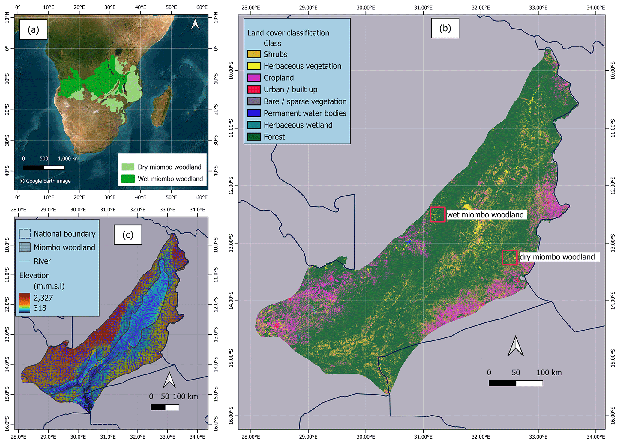
Figure 1 (a) Spatial extent of the miombo woodland in Africa and the location of the Luangwa Basin in Zambia. (b) Land cover characterisation of the Luangwa Basin based on the Copernicus Land Cover classification. (c) Spatial distribution of elevation from the Advanced Spaceborne Thermal Emission and Reflection radiometer (ASTER) global digital elevation model (GDM) version 3 and the extent of the miombo woodland in the Luangwa Basin.

2.2 Study approach

The study sought to find out the extent to which satellite-based evaporation estimates agree with each other during the different canopy phenophases of the miombo woodland. Point-scale observations in the wet miombo woodland (Zimba et al., 2023) showed that satellite-based evaporation estimates underestimated actual evaporation of the wet miombo woodland during the dry season and early rainy season in the Luangwa Basin. However, the Luangwa Basin has a heterogenous land cover, which includes mopane woodland and grasslands. The question was whether the heterogeneity in the land cover of the Luangwa Basin would result in satellite-based evaporation estimates performing contrary to the point-scale observations at a wet miombo woodland site when compared to the water-balance-based evaporation estimates at the basin scale.

For this study, a 12-year period, 2009–2020, was used because satellite-based evaporation estimates were available for free for this period. The period also had cycles of low and high annual rainfall, allowing for the analysis performance under changing monthly and annual conditions. The following sections elaborate the methods used in this study.

2.2.1 Phenophases of the miombo woodland and assessment of phenological conditions

To categorise the phenophases, two approaches were used: climate-and-soil-moisture-based classifications and satellite-based classifications. For the climate-and-soil-moisture-based classification (Chidumayo and Frost, 1996), five phenological seasons were observed: the warm pre-rainy season, early rainy season, mid-rainy season, late rainy season, and cool-dry season (Fig. 2). For ease of analysis, the above three rainy-season phenophases were merged into one rainy-season phenophase. Therefore, three climate-and-soil-moisture-based phenophases were established: the warm pre-rainy season, rainy season, and cool-dry season. The satellite-based classification of phenophases was based on the National Aeronautics and Space Administration (NASA) Collection 6 MODIS Land Cover Dynamics (MCD12Q2) product, which can be accessed at https://modis.ornl.gov/globalsubset/ (last access: 20 February 2023; Gray et al., 2019; Zhang et al., 2003). The MCD12Q2 uses the changes in canopy greenness to characterise the canopy phenophases (Gray et al., 2019). For the miombo woodland in the Luangwa Basin, eight phenophases were identified using the satellite-based MCD12Q2 data (Fig. 2). The satellite-based phenophases are green-up, mid-green-up, maturity, peak, senescence, green-down, mid-green-down, and dormant. For ease of analysis, the phenophases were merged into four groups based on the dominant activity in each phenophase (Fig. 2). To complement the MCD12Q2 classification, the MODIS-based leaf area index (LAI), obtained from https://modis.ornl.gov/globalsubset/, last access: 20 February 2023, Myneni et al., 2021; ORNL DAAC, 2018), and the normalised difference vegetation index (NDVI) (ORNL DAAC, 2018; Vermote and Wolfe, 2015) were used.

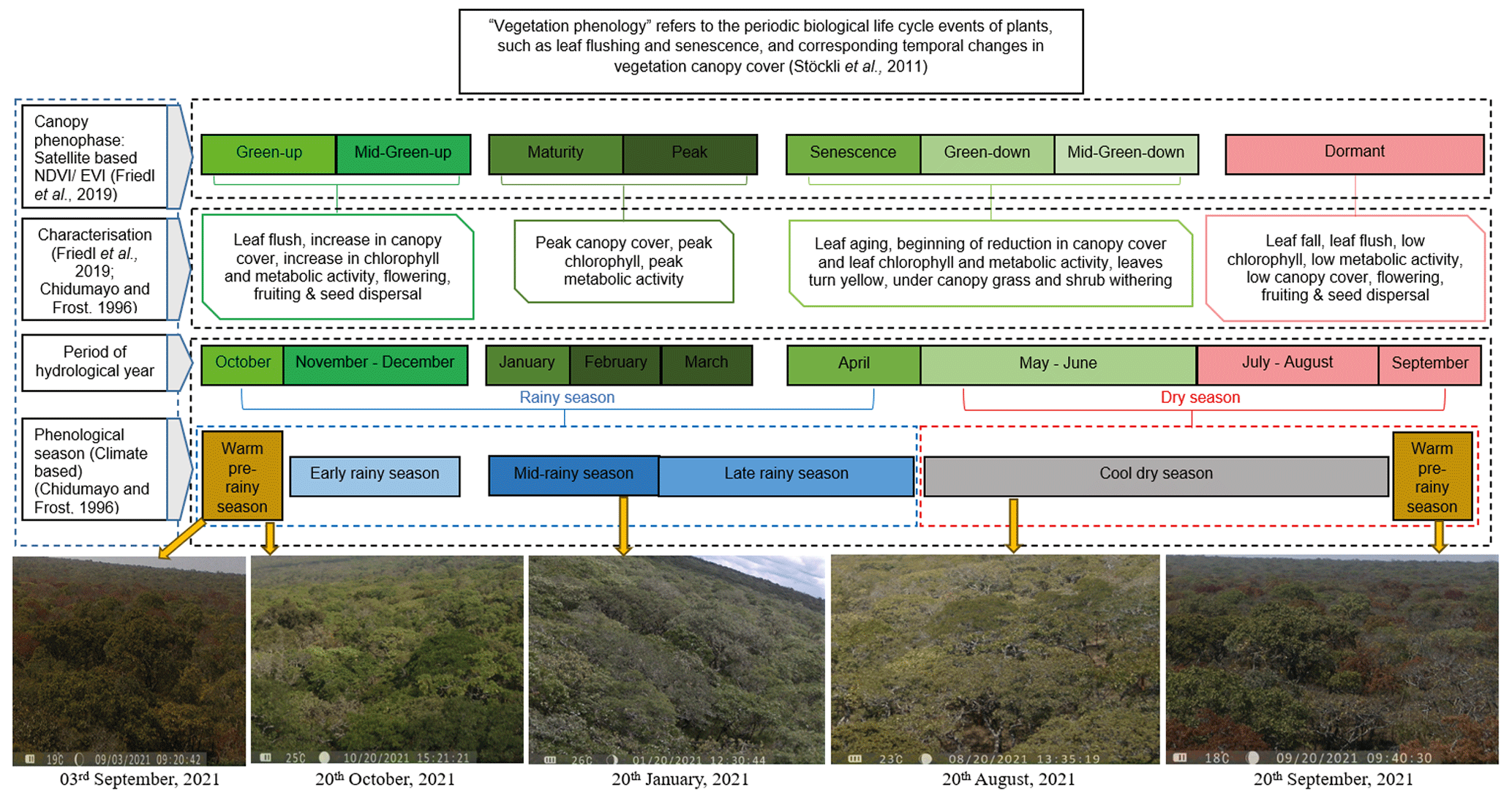
Figure 2 Characterisation of canopy phenophases of the miombo woodland in relation to seasonality for the Luangwa Basin. Photographs show the changes in the canopy cover on selected days across different phenophases of a wet miombo woodland at the Mpika site (12.387454° S, 31.170911° E) for the year 2021.

The satellite-based LAI and NDVI have been used before as proxies to observe phenological conditions, such as the canopy biomass formation, changes in the canopy closure (i.e. through leaf fall and leaf flush), and changes in canopy chlorophyll conditions (Guan et al., 2014; Santin-Janin et al., 2009; Chidumayo, 2001; Fuller, 1999). For the LAI, the NASA's MCD15A3H product (Myneni et al., 2021; ORNL DAAC, 2018), with a 4 d temporal resolution and 500 m spatial resolution, was used. The MODIS MOD09GQ.006 (Vermote and Wolfe, 2015) surface reflectance bands 1, 5, and 6 were used to estimate the NDVI at a daily temporal resolution and 250 m spatial resolution using the band ratio method. The daily NDVI values were then averaged into 4 d values to obtain the same temporal resolution as that of the LAI.

To mitigate potential confusion that arises from the use of dual phenophase classifications, this study exclusively employs satellite-based phenophases for analysis purposes. Within these phenological seasons, the phenology of miombo species transitions through various stages, i.e. from leaf fall and leaf flush, growth of stems, and flowering to mortality of seed (Chidumayo and Frost, 1996). To complement the observations, photographs from a digital camera (Denver WCT-8010) installed on the flux tower at a wet miombo woodland site in Mpika (Zimba et al., 2023) were used to observe the changes in the canopy phenology of the miombo woodland across different phenophases from January to December in the year 2021. In addition, a fish-eye lens (LIEQI LQ-001) was used to obtain canopy images. The images of the canopy helped to observe the changes and differences in canopy leaf display (i.e. leaf fall, leaf flush, and leaf colour changes) among miombo species.

2.2.2 Delineation of the miombo woodland areas used in this study

The satellite-based evaporation estimates were compared to each other using grids at two known sites representing the dry miombo woodland and wet miombo woodland and at the entire miombo woodland scale in the Luangwa Basin (Figs. 1 and 3).

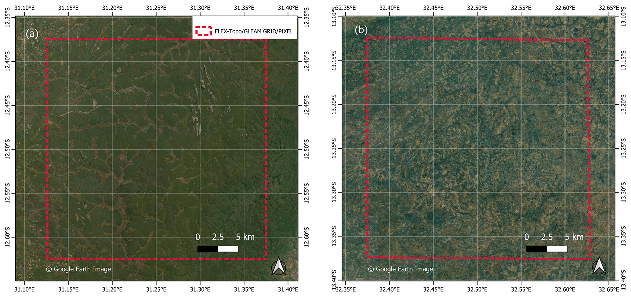
Figure 3 The wet miombo woodland (a) and dry miombo woodland (b) locations used for comparison of satellite-based evaporation estimates at FLEX-Topo and GLEAM spatial resolution (approximately 27.7 km by 27.7 km). The dashed red line is the actual location of the FLEX-Topo and GLEAM pixels.

Firstly, a comparison based on the 27.7 km by 27.7 km grid was performed using known undisturbed dry miombo woodland and wet miombo woodland locations (Figs. 1 and 3). The grid was based on the satellite-based evaporation estimates (i.e. the Topography-driven Flux Exchange, FLEX-Topo, and Global Land Evaporation Amsterdam Model, GLEAM) with the largest spatial resolutions (approximately 27.7 km by 27.7 km) (Fig. 3 and Table 1). For the Moderate-Resolution Imaging Spectrometer (MODIS) MOD16, Simplified Surface Energy Balance (SSEBop), Thornthwaite–Mather Climatic Water Balance (TerraClimate), and Water Productivity through Open access of Remotely sensed derived data (WaPOR), the mean of aggregated actual evaporation estimates in all the pixels within the dashed red square (Fig. 3) were used in the same way the mean of the aggregated NDVI and LAI values in all the pixels within the dashed red square were used for analysis. The focus on a known wet miombo woodland enabled comparison of the field observations of the changes in canopy cover using digital camera images to the satellite-based LAI and NDVI for the year 2021. See Sect. 2.2.3 and Table 1 for satellite-based evaporation estimates used in this study. Secondly, the typical miombo woodland regions, as categorised by White (1983) and Ryan et al. (2016) (see Fig. 1a, b), were used to delineate the area covered by the miombo woodland in the Luangwa Basin. The delineated miombo woodland in the Luangwa Basin excluded the mopane woodland, mixed woodland, and waterbodies. This delineation (as shown in Fig. 1) ensured that only the areas classified as typical miombo woodland (Ryan et al., 2016; White, 1983) were considered in the analysis.

2.2.3 Satellite-based products used in the study

The six satellite-based evaporation estimates consisted of the (1) Topography-driven Flux Exchange (FLEX-Topo) model (Hulsman et al., 2021, 2020; Savenije, 2010), (2) Thornthwaite–Mather Climatic Water Balance (TerraClimate) dataset (Abatzoglou et al., 2018), (3) Global Land Evaporation Amsterdam Model (GLEAM) (Martens et al., 2017; Miralles et al., 2011), (4) Moderate-Resolution Imaging Spectrometer (MODIS) MOD16 product (Running et al., 2019; Mu et al., 2011, 2007), (5) operational Simplified Surface Energy Balance (SSEBop) model (Senay et al., 2013), and (6) Water Productivity through Open access of Remotely sensed derived data (WaPOR) (FAO, 2020). These satellite-based evaporation estimates were selected purely because they are free of charge, are easily accessible from various platforms, and have an archive of historical data with the temporal and spatial resolutions suitable for use in this study. Except for FLEX-Topo and GLEAM (with a spatial resolution of 27.7 km), these satellite-based evaporation estimates have relatively fine spatial resolution (i.e. 500, 1000, 4000, and 250 m for MOD16, SSEBop, TerraClimate, and WaPOR respectively) and temporal resolution (1 d, 8 d, 10 d, and monthly respectively), which are attributes that were suitable for this study. The original spatial resolutions were used because these satellite-based evaporation estimates are normally used as is, in their original resolutions. Resampling the different spatial resolutions of the satellite-based evaporation estimates to a single (uniform) spatial resolution was thought to be problematic as it would have introduced unknown and unquantifiable errors regardless of the extent to which it is resampled. For detailed explanations of the model structure, processes, and inputs for the satellite-based evaporation estimates used in this study, the reader is advised to refer to the cited literature above and in Table 1.

Other satellite-based products used in this study include the ASTER digital elevation model (DEM) (NASA/METI/AIST/Japan Space Systems and US/Japan ASTER Science Team, 2019), MODIS-based LAI and NDVI, Copernicus Land Cover map, net radiation, precipitation, runoff, soil moisture, and relative humidity. For detailed information (i.e. structure, processes, and inputs) on the other satellite-based products used in this study, the reader is advised to refer to the literature cited in Table 1.

Table 1 Characteristics of products used in the study.

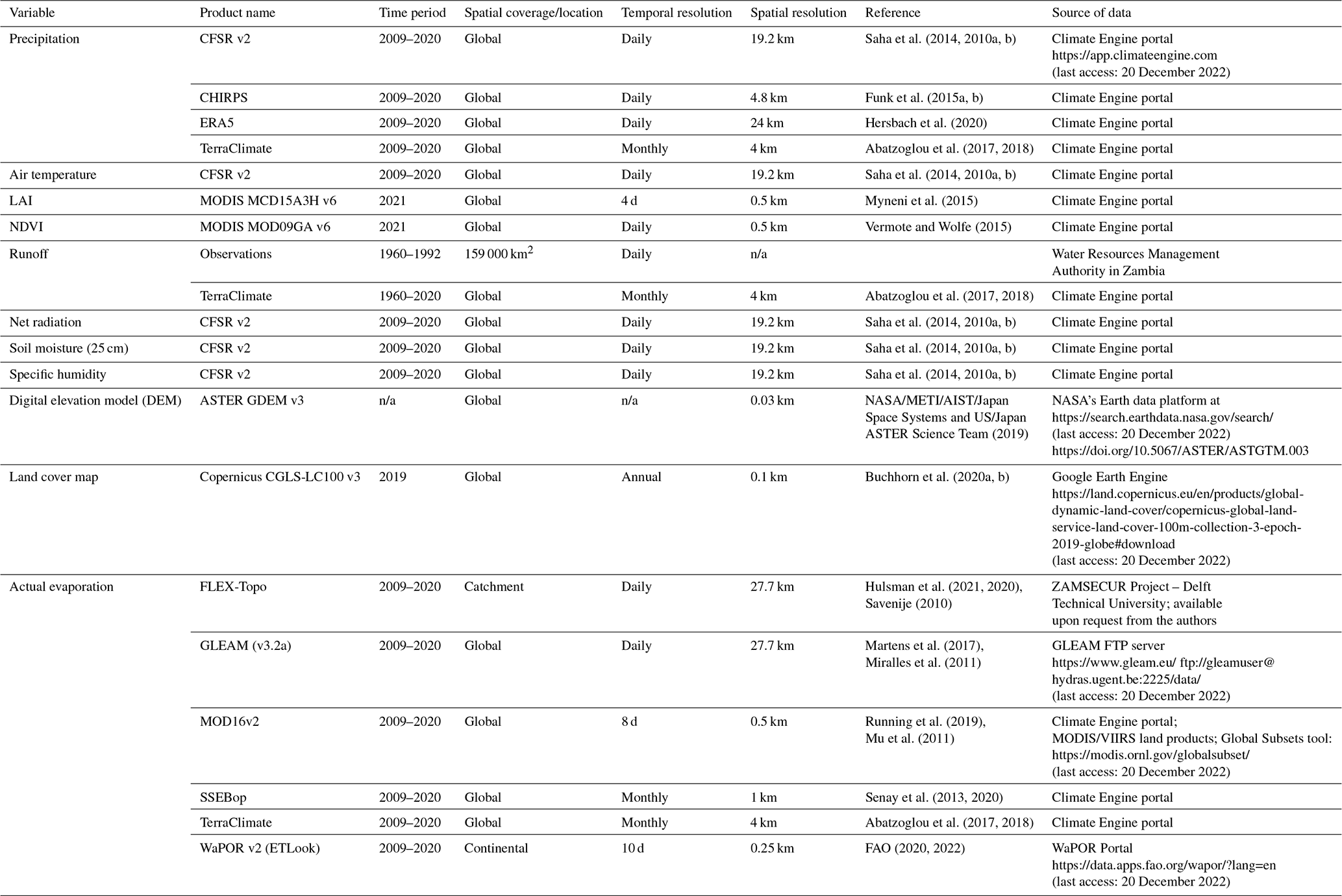
CFSR v2: Climate Forecasting System Reanalysis version 2. CHIRPS v2: Climate Hazards Group InfraRed Precipitation with Station data version 2. ERA5: European Centre for Medium-Range Weather Forecasts reanalysis 5.
ASTER GDEM v3: Advanced Spaceborne Thermal Emission and Reflection radiometer global digital elevation model version 3. LAI: leaf area index. NDVI: normalized difference vegetation index. CGLS-LC: Copernicus
Global Land Services – Land Cover. VIIRS: Visible Infrared Imaging Radiometer Suite. MCD: MODIS Land Cover Dynamics. FLEX-Topo: Topography-driven Flux Exchange. n/a: not applicable.

2.2.4 Actual evaporation derived from the water balance

In cases where spatially distributed field measurements are not available, the water balance approach, using spatially distributed satellite data, is a possible practical approach (i.e. Weerasinghe et al., 2020; Liu et al., 2016). In this study, the general annual water balance was used to test the performance of the satellite-based evaporation estimates at the basin level.

The basin average annual water-balance-based evaporation ($E_{{\mathrm{a}}_{\left(\mathrm{wb}\right)}}$) is estimated using Eq. (1), where long-term over-year storage change is disregarded.

$$\begin{array}{}\text{(1)}& E_{{\mathrm{a}}_{\left(\mathrm{wb}\right)}}=P-Q,\end{array}$$

where P is the annual average catchment precipitation in millimetres per year and Q is the annual average discharge in millimetres per year. The precipitation and discharge information for the water balance approach were selected and used as explained below.

Ensemble satellite precipitation

The challenge posed by satellite-based precipitation data in African catchments is that most, if not all, satellite precipitation products are geographically biased towards either underestimation or overestimation despite some of them having a good correlation with ground observations (Macharia et al., 2022; Asadullah et al., 2008). The lack of adequate ground precipitation observations makes it difficult to validate, as well as correct, the product's bias with an acceptable degree of certainty. There is not a single precipitation product that has been found to perform better than other precipitation products across African landscapes and southern Africa in particular (Macharia et al., 2022). For the Luangwa Basin, there is no guarantee that any of the precipitation products are spatially representative of a basin that is the size of about 159 000 km² with varying topographical attributes. For instance, compared to point-based field observations of precipitation at six weather stations in Zambia (three stations in the Luangwa Basin and the other three outside of the Luangwa Basin), no single satellite-based precipitation product showed consistency with all weather stations (see Table S1). Using an ensemble of precipitation products is said to reduce errors and is therefore recommended (e.g. Weerasinghe et al., 2020; Asadullah et al., 2008). When the annual mean of an ensemble of four satellite-based precipitation products was compared to annual means of field observations at different weather stations, the margin of either underestimation or overestimation was reduced (see Table S1). To this extent, for the general water balance, this study used annual mean of four satellite precipitation products. The four precipitation products are the Climate Forecasting System Reanalysis (CFSR), Climate Hazards Group Infrared Precipitation with Station data (CHIRPS), ECMWF reanalysis v5 (ERA5), and TerraClimate (see Table 1). These satellite precipitation products were selected purely based on availability and the fact that they are spatially distributed and cover the entire Luangwa Basin (Table 1). Field observations of precipitation for Golden Valley Agriculture Research Trust (GART) Chisamba (data for the period 2020–2022), Lusaka International Airport, Kabwe, Mwinilunga, and Serenje weather stations for the years 2014–2016 were obtained from the Southern African Science Service Centre for Change and Adaptive Land Management (SASSCAL) weather network (http://www.sasscalweathernet.org, last access: 20 January 2023). The observations for Mpika for the year 2021 were obtained from the ZAMSECUR project dataset available on the 4TU.ResearchData repository (https://doi.org/10.4121/19372352.v2; Zimba et al., 2022). Three weather stations, GART Chisamba, Lusaka International Airport, and Mwinilunga, are outside of the Luangwa Basin and were used for comparison purposes only. However, the GART Chisamba and Lusaka International Airport stations are very close to the Luangwa Basin. The other three stations, Kabwe, Serenje, and Mpika, are within the Luangwa Basin (see Table S1 for location coordinates of the weather stations). Nevertheless, the results of the comparison of satellite precipitation products with field observations were similar (underestimation or overestimation) at all weather stations, both in the Luangwa Basin and outside the basin (see Table S1).

Estimating runoff data

Reliable monthly basin-scale field observations of runoff were only available for the period 1961–1992 and not for the study period 2009–2020. Monthly modelled TerraClimate runoff data (Abatzoglou et al., 2018) were available for the period 1958–2020. The shapefile for the entire Luangwa Basin was used as a boundary for the gridded TerraClimate runoff and to obtain the basin-scale average runoff. The basin-scale average of TerraClimate runoff was then compared with the observed Luangwa Basin runoff. Compared to field observations, the average TerraClimate runoff data were significantly higher during the peak rainfall period of January–February. At the annual scale, TerraClimate overestimated runoff data but its results were strongly correlated (r= 0.83) with field observations (Fig. 4a).

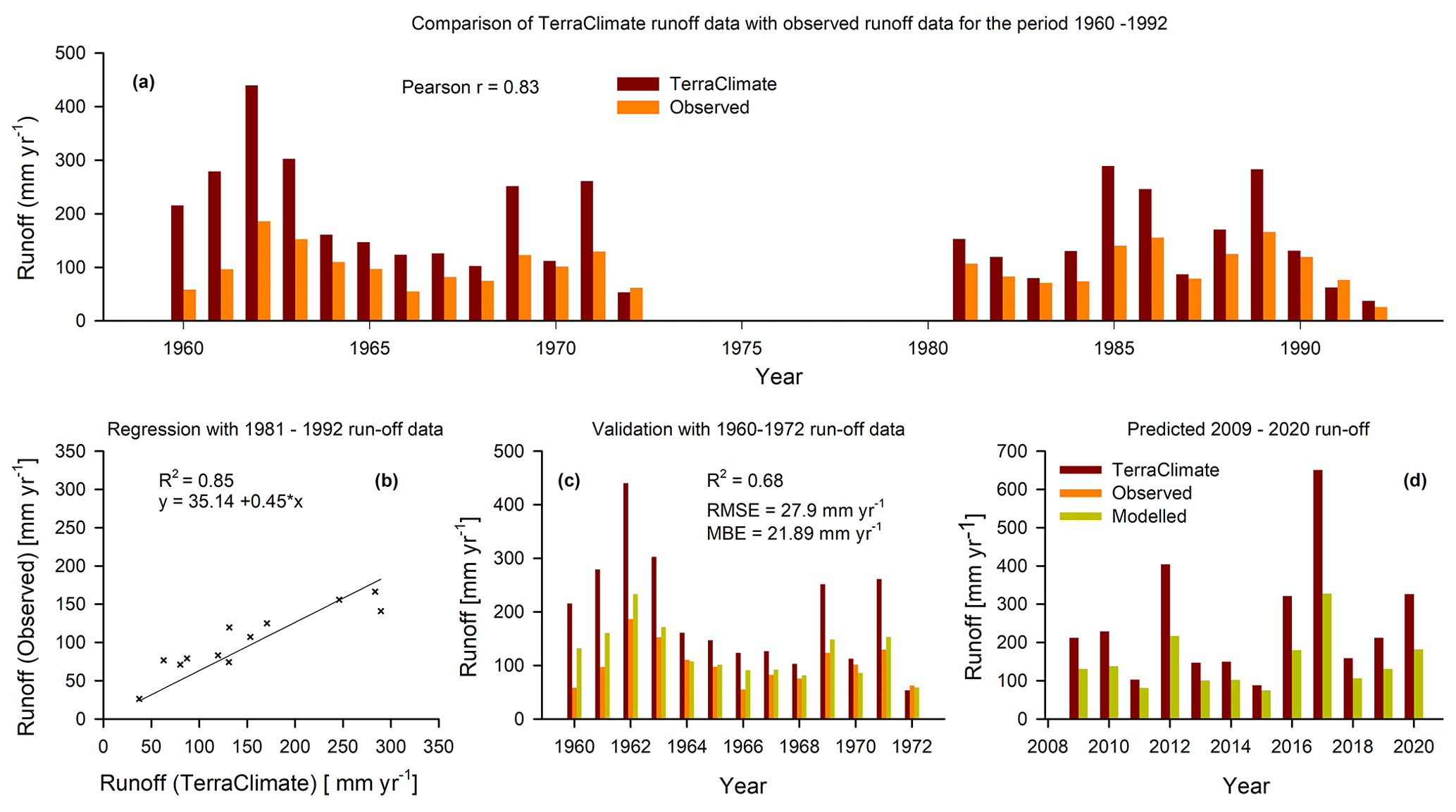
Figure 4 Procedure for extending near-field observation runoff data for the period 2009–2020 using the TerraClimate runoff data as the predictor. (a) Annual time series of observed runoff and TerraClimate runoff for the period 1960–1992, (b) regression of observed runoff with TerraClimate runoff for the period 1981–1992, (c) validation of the regression model for predicting runoff using the 1960–1972 observed runoff data, and (d) comparison of predicted TerraClimate runoff using the regression model with original TerraClimate runoff time series.

Based on the correlation of annual TerraClimate runoff data with field observations, a linear regression equation was formulated to help generate extended near-field observation time series for the period 2009–2020. TerraClimate runoff data were used as predictor variable. The TerraClimate runoff data were used because of their availability free of cost and their relatively fine temporal and spatial resolution (monthly and 4 km respectively) (Table 1). Firstly, the field observation runoff data and TerraClimate runoff data for the period 1960–1992 were split into two segments, 1960–1972 and 1981–1992. The runoff data for the period 1981–1992 were used as training data to generate a linear equation with the TerraClimate runoff data as the predictor variable (Fig. 4b). The generated linear equation was validated using the 1961–1972 TerraClimate runoff data as a predictor variable (Fig. 4c). The predicted 1961–1972 runoff data with the TerraClimate runoff data as a predictor variable were then compared to the field observations for the same period (Fig. 4c). The performance statistics of the equation showed that R²= 0.68, RMSE = 27.9 mm yr⁻¹ and mean bias error (MBE) = 21.9 mm yr⁻¹ (Fig. 4c). The linear regression equation was then used to generate near-field observation runoff data for the period 2009–2020 with TerraClimate runoff data for the same period as the predictor variable (Fig. 4d). Generally, both for the observed and extended time series (with TerraClimate data as the predictor), the annual runoff coefficient was 11 %. The near-field observation extended runoff data were then used in the water balance approach, as explained in Eq. (1) in Sect. 2.2.4, to estimate actual evaporation at the basin level.

2.2.5 Time series pre-processing and statistical analyses

Deseasonalising time series

The presence of seasonal variations in hydrological time series can complicate data analysis and hinder the identification of underlying trends and patterns. Deseasonalising (removing seasonality from) the data can provide a clearer understanding of its long-term behaviour and prevent false results. The centred moving average (CMA) and adjusted seasonal factor (ASF) are among the various commonly used methods of deseasonalising time series (Ghysels et al., 2006; Nelson et al., 1999; Briuinger et al., 1983). To prepare for statistical analyses, the original time series of evaporation, LAI, and NDVI were deseasonalised using the CMA and ASF approaches. Firstly, the time series were examined for the presence of seasonality. Once a 12-month lag of the seasonal component was detected, the time series were deseasonalised. This involved calculating the CMA using Eqs. (2) and (3). The ASF was estimated by dividing the original time series by the CMA, as indicated in Eq. (4). Then, the original monthly time series were deseasonalised by dividing them by the ASF of each variable, as given in Eq. (5).

$$\begin{array}{}\text{(2)}& \begin{array}{rl}& X_{t+\mathrm{0.5}}^{*}={\sum }_{j=-\left(\frac{S}{\mathrm{2}}\right)+\mathrm{1}}^{S/\mathrm{2}}{X}_{t+j},\\ & t={\displaystyle \frac{S}{\mathrm{2}}},{\displaystyle \frac{S}{\mathrm{2}}}+\mathrm{1},{\displaystyle \frac{S}{\mathrm{2}}}+\mathrm{2},\mathrm{\dots }..,n-{\displaystyle \frac{S}{\mathrm{2}}}\end{array}\end{array}$$

To estimate a centred moving average ($X_t^{*}$) Eq. (3) is used.

$$\begin{array}{}\text{(3)}& {\displaystyle }{X}_t^{*}={\displaystyle \frac{X_{t-.5}^{*}+X_{t+\mathrm{0.5}}^{*}}{\mathrm{2}}},t={\displaystyle \frac{S}{\mathrm{2}}},{\displaystyle \frac{S}{\mathrm{2}}}+\mathrm{1},{\displaystyle \frac{S}{\mathrm{2}}}+\mathrm{2},\mathrm{\dots },n-{\displaystyle \frac{S}{\mathrm{2}}},\text{(4)}& {\displaystyle }\mathrm{ASF}={\displaystyle \frac{X_t}{X_t^{*}}},\text{(5)}& {\displaystyle }{X}_{\mathrm{td}}={\displaystyle \frac{X_t}{\mathrm{ASF}}},\end{array}$$

where X_t is the original variable estimate for each month, ($X_{t+\mathrm{0.5}}^{*}$) is the moving average value, $X_t^{*}$ is the centred moving average value, S is the even number of the lag of the seasonal component (12 in the case of this study), n is the total number of time series, ASF is the adjusted seasonal factor, and X_td is the deseasonalised time series. In order to assess the degree of deviation between original time series and deseasonalised time series with the purpose of identifying anomalous occurrences within the data, the original monthly time series were subtracted by the deseasonalised time series (Eq. 6).

$$\begin{array}{}\text{(6)}& \mathrm{anomaly}=X_t-X_{\mathrm{td}}\end{array}$$

Therefore, for statistical analyses, the original time series, the deseasonalised time series, and the anomalies were utilised in this study.

Statistical analyses

The Mann–Kendall trend test (Helsel et al., 2020), a non-parametric statistical model, was used to evaluate the overall temporal trend in satellite-based evaporation estimates. The coefficient of variation (CV) (in %) in Eq. (7) (Helsel et al., 2020) was used to understand the extent to which the satellite-based evaporation estimates varied between each other for each phenophase. When evaluating temporal variations in individual satellite-based evaporation estimates, high coefficients of variation (CVs) in certain phenophases may not necessarily indicate uncertainties in estimating evaporation. Instead, they could be a result of temporal variations in climate variables such as leaf area, rainfall, soil moisture, and temperature. On the other hand, when comparing the means of different satellite-based evaporation estimates over a specific phenophase, high CV values indicate larger differences between the means of individual evaporation estimates. In this case, these high CVs may be indicative of differences in the ability of individual satellite-based approaches to estimate evaporation in that phenophase.

$$\begin{array}{}\text{(7)}& \mathrm{CV}={\displaystyle \frac{\stackrel{\mathrm{‾}}{x}}{\stackrel{\mathrm{‾}}{s}}},\end{array}$$

where $\stackrel{\mathrm{‾}}{x}$ is the mean of the observations and $\stackrel{\mathrm{‾}}{s}$ the standard deviation. The higher the CV value, the larger the standard deviation compared to the mean, which implies greater variation among the variables.

Furthermore, the analysis of variance (ANOVA) (Helsel et al., 2020) and all pairwise multiple comparison procedures were performed with the Tukey test (Helsel et al., 2020). The ANOVA and the pairwise comparison assisted in observing the satellite-based evaporation estimates that were significantly different in magnitudes in each phenophase. The study examined the correlations between satellite-based evaporation estimates, specifically focusing on their similarity in temporal dynamics. This assessment was conducted at both monthly and annual scales using two different techniques: the non-parametric Kendall correlation test (Helsel et al., 2020) and the parametric Pearson correlation (Helsel et al., 2020). The choice between these two techniques depended on the results of the normality test conducted on the time series data. To establish the extent to which the satellite-based evaporation estimates underestimated or overestimated evaporation relative to E_wb, the mean bias error (Eq. 8) is used:

$$\begin{array}{}\text{(8)}& \mathrm{MBE}={\displaystyle \frac{\mathrm{1}}{n}}{\sum }_{i=\mathrm{1}}^n\left(E_{{\mathrm{s}}_i-}{E}_{{\mathrm{a}}_{(\mathrm{wb}{)}_i}}\right),\end{array}$$

where n is the number of annual data items used, $E_{{\mathrm{a}}_{\left(\mathrm{wb}\right)}}$ is the water-balance-based actual evaporation time series, and E_s is the satellite-based evaporation estimate time series. The smaller the mean bias error value (positive or negative), the lower the deviation of the predicted values from the water balance obtained values (Helsel et al., 2020).

3 Results and discussion

3.1 Basin-scale miombo woodland climate and phenological temporal dynamics(s)

Figure 5 shows the Luangwa Basin miombo woodland (area delineated as miombo woodland only in Fig. 1c) aggregated 2009–2020 MODIS NDVI and CFSR data climate conditions: net radiation (R_N), air temperature (T_a), relative humidity (RH), soil moisture (SM), and precipitation (P). The peak atmospheric and phenological variables values were observed in the early and mid-rainy seasons during the green-up and maturity and peak phenophases. The lowest values in atmospheric and phenological variables were observed in the cool-dry season during the green-down and dormant phenophases. Net radiation, air temperature, and relative humidity covaried (positively or negatively) with the NDVI (proxy for canopy phenology) depending on the phenophase (Figs. 5 and S2).

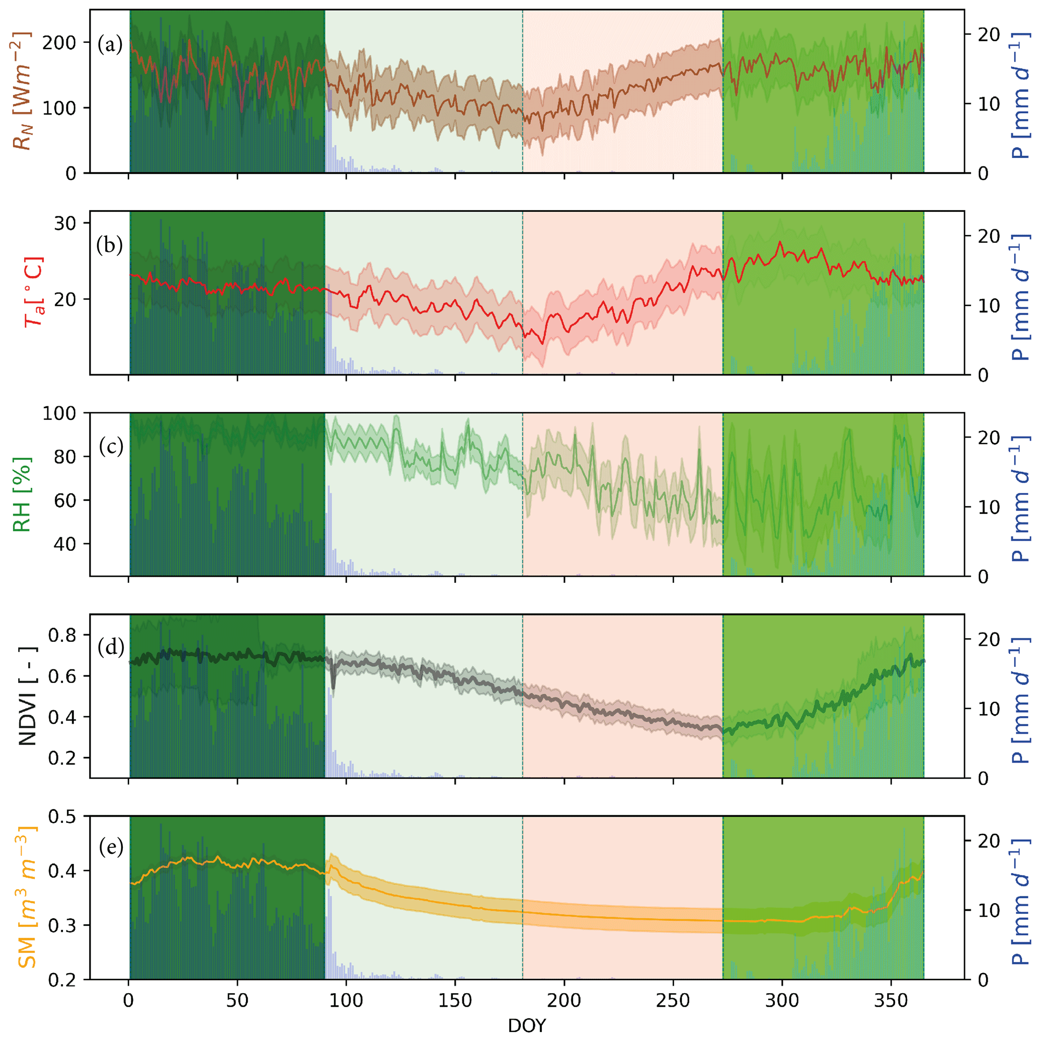
Figure 5 Luangwa Basin miombo woodland spatially and temporally aggregated 2009–2020 daily atmospheric conditions: (a) net radiation (R_N), (b) air temperature (T_a), (c) relative humidity (RH), (d) phenological conditions proxied by the NDVI, and (e) soil moisture (SM) plotted against precipitation (P). The shaded areas represent the phenophases as used in this study: January–March is the peak and maturity, April–June is the senescence and green-down, July–September is the dormant, and October–December is the green-up and mid-green-up phenophases. The shaded area for variables is the standard deviation. DOY is the day of the year.

The strong correlation between climate and phenology (i.e. NDVI and air temperature/soil moisture) in the miombo woodland (Fig. S2) agreed with observations made by Chidumayo (2001) and in other ecosystems (Pereira et al., 2022; Schwartz, 2013; Cleland et al., 2007).

3.2 Observed phenological conditions in the miombo woodland

Fuller (1999) observed that the canopy closure is varied, ranging between 2 % and about 70 % in the shrub, dry miombo woodland, and wet miombo woodland. Therefore, depending on the location and dominant species, exposure of the understorey, field, and ground layers to incident solar radiation through the canopy is substantial (Fig. 6, Chidumayo, 2001; Fuller, 1999).

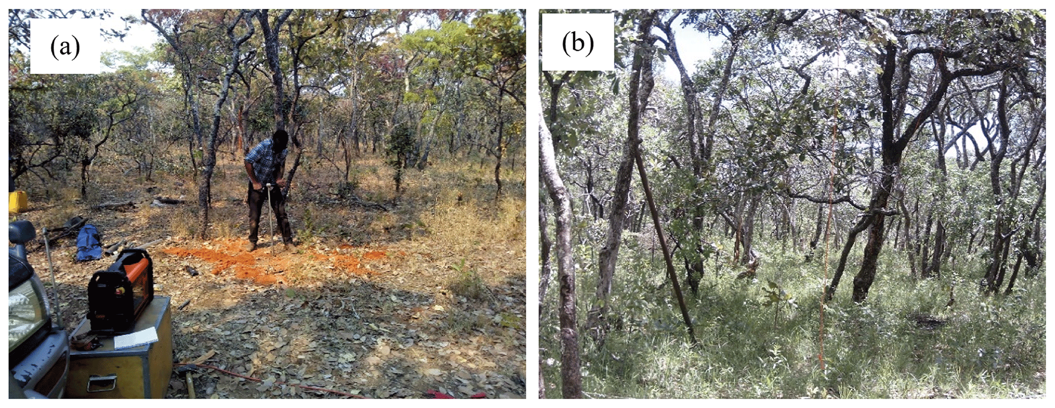
Figure 6 Dry-season (a) and rainy-season (b) tree layer, understorey, and field layer conditions at the wet miombo woodland site (12.387454° S, 31.170911° E) in Mpika, Zambia. Images were taken on 29 September and 23 December 2021.

In the dry season, the grass in the field layer and some understorey non-deep-rooting shrubs die when moisture is scarce. During dry periods, they survive by entering a dormant state, with buds located near the soil surface (Fig. 6a and Chidumayo, 2001; Fuller, 1999). Hence, the changes in total LAI and NDVI in the phenophases in the dry season can largely be attributed to the changes in the tree layer of the miombo species (i.e. Figs. 6a and 7 and Chidumayo, 2001). The field layer during the rainy season mainly comprises green grass (Fig. 6b and Chidumayo, 2001). Therefore, total LAI and NDVI in phenophases in the rainy season can be largely attributed to both the field layer, i.e. grass and understorey, and the tree layer, i.e. shrubs and tree canopy (i.e. Fig. 6b and Chidumayo, 2001). The LAI and NDVI were used as proxies to observe the changes in the canopy cover across different phenophases of the miombo woodland. At a 27.7 km-by-27.7 km grid scale (Fig. 8a), the spatial distribution and mean of the aggregated values of the LAI and NDVI for the dry miombo woodland differed from that of wet miombo woodland (Fig. 8a). This difference is due to the differences in species composition and distribution at each site. Furthermore, there are differences in soil type, soil moisture, temperature, nutrients, rainfall, and canopy closure at the two sites (i.e. Chidumayo, 2001; Fuller, 1999). However, temporal variations in the mean of aggregated LAI and NDVI values across different phenophases of the miombo woodland at the two sites were similar (r= 0.78 and 0.76 for LAI and NDVI respectively) (Fig. 8c). Highest mean LAI and mean NDVI, both in the dry miombo woodland and wet miombo woodland, were observed in the maturity and peak phenophases during the mid-rainy season (January–March) (Figs. 5, 7i, 8c, and S3).

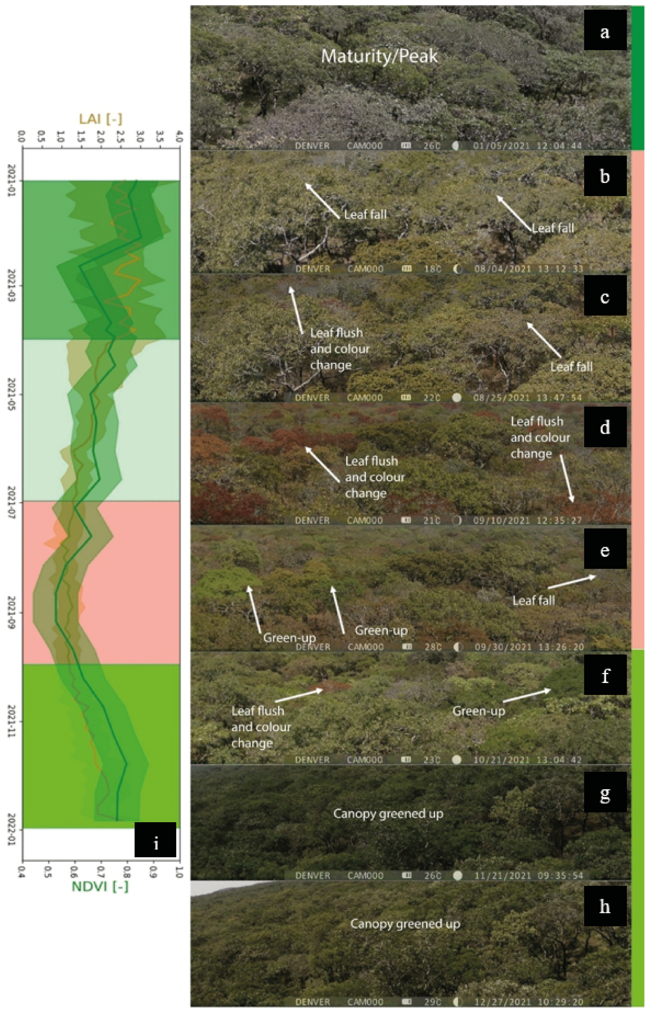
Figure 7 The wet miombo woodland canopy display trend for the year 2021 at the Mpika study site (12.387454° S, 31.170911° E): (a) 5 January, (b) 4 August, (c) 25 August, (d) 10 September, (e) 30 September, (f) 21 October, (g) 21 November, and (h) 27 December. Shaded area are phenophases: January–March is the maturity and peak, April–June is the senescence and green-down, July–September is the dormant, while October–December is the green-up and mid-green-up phenophase. (i) Temporal dynamics of MODIS LAI and NDVI (the shaded area for variables is the minimum and maximum). Emphasis was placed on the dormant and the green-up and mid-green-up phenophases when major changes in canopy display occurs.

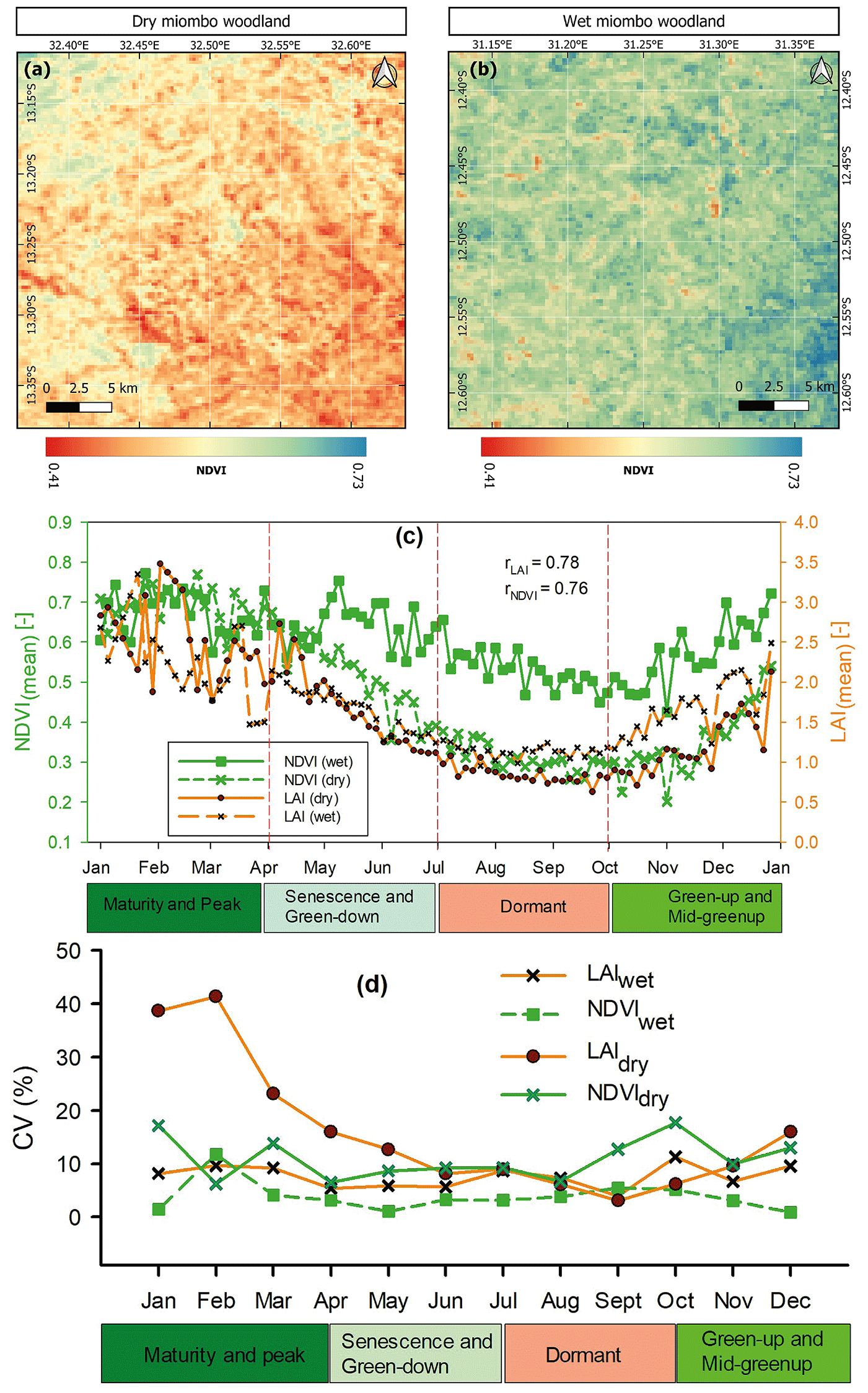
Figure 8 Spatial distribution of mean NDVI at the (a) dry miombo woodland and (b) wet miombo woodland site for the period January–December, 2021. (c) Temporal distribution of the mean of the aggregated LAI values and aggregated NDVI values for the wet miombo woodland and dry miombo woodland. (d) Temporal coefficients of variation in the mean LAI and NDVI values at the wet miombo woodland and dry miombo woodland in the Luangwa Basin in Zambia for the year 2021.

The maturity and peak period corresponds to the peak LAI and NDVI (Figs. 7 and 8), as noted by Chidumayo (2001). According to Chidumayo (2001), the miombo woodland experiences the highest green biomass between January and May. On the contrary, the dormant phenophase in August and September, which occurs during the warm pre-rainy season, exhibited the lowest LAI and NDVI values (Figs. 5, 7, and 8). This period is characterised by leaf fall, leaf flush, and changes in leaf colour (Figs. 7 and 9; Chidumayo, 2001; Chidumayo and Frost, 1996; Fuller, 1999).

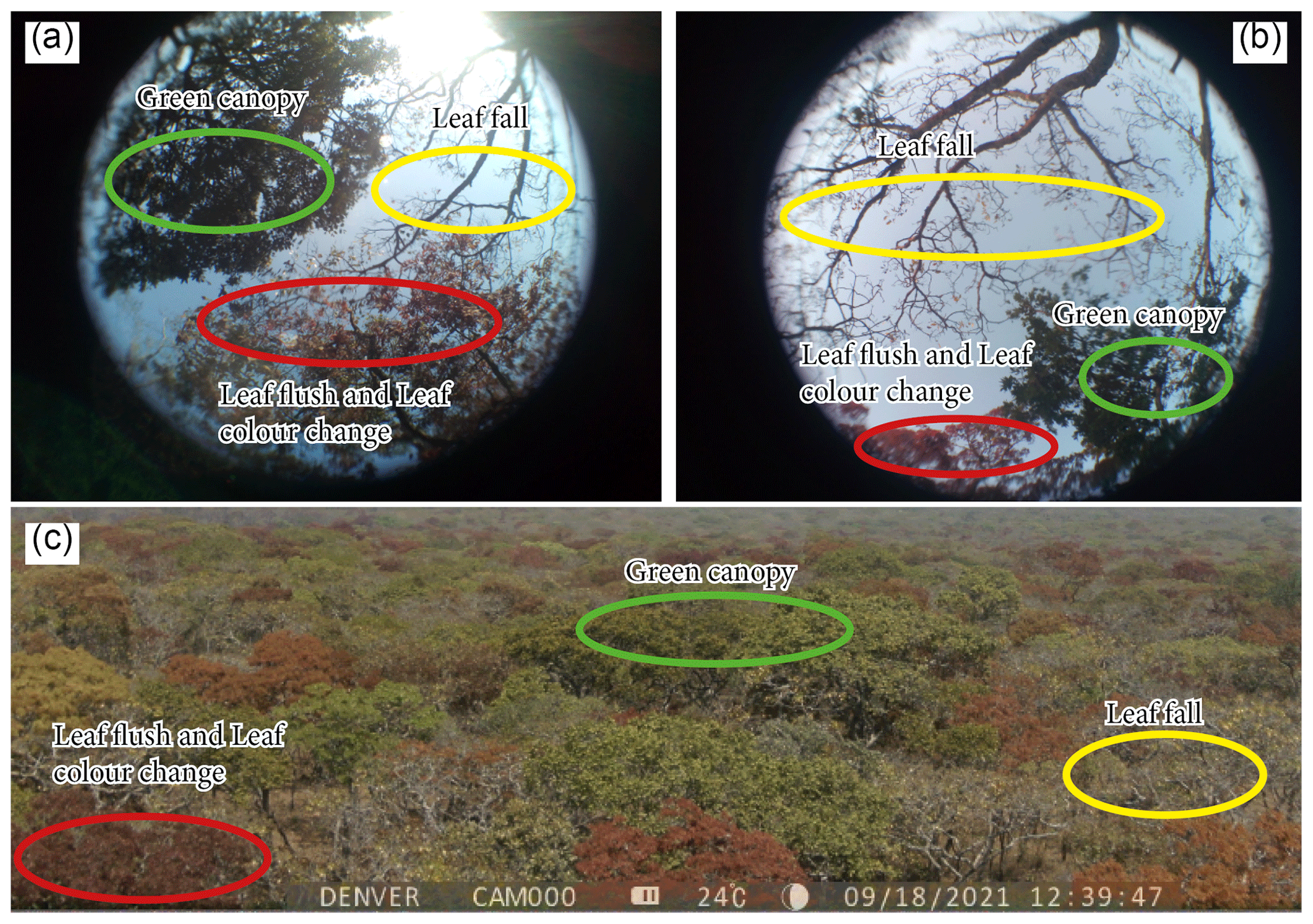
Figure 9 Heterogeneity in leaf-fall and leaf-flush activities among miombo woodland species, as observed from under the canopy (a, b) and as observed from above the canopy (c). Images were taken at the wet miombo woodland site (12.387454° S, 31.170911° E) in Mpika, Zambia. Images were taken on 18 September 2021.

Table 2 presents the correlation coefficients for the temporal coefficients of variation in within-month variations in the means of the aggregated NDVI and LAI values for the dry miombo woodland and wet miombo woodland. The only period in which both LAI and NDVI values had significantly higher correlation coefficients (r= 0.97 for LAI and r= 0.75 for NDVI) in the temporal coefficients of variation for the dry miombo woodland and wet miombo woodland is the dormant phenophase (Fig. 8 and Table 2). This similarity in the coefficients of variation can be attributed to the plants undergoing similar phenological processes, such as leaf fall and leaf flush, during the dormant phase. During this phase, the grass component dries out, leaving only the tree component (i.e. the canopy) to determine the leaf area (Chidumayo, 2001). The increased temporal variations in NDVI values in August–September (Figs. 8d and 9) may also be explained by intensified leaf fall, leaf flush, and leaf colour changes. Increased leaf-fall activity can account for the temporal coefficients of variation in mean LAI values in July and August for the wet miombo woodland (Figs. 8 and 9).

Table 2 Correlation coefficients (alpha value = 0.05) of the temporal coefficients of variation values of the within-month variations in the means of aggregated LAI and NDVI for the dry miombo woodland and wet miombo woodland.

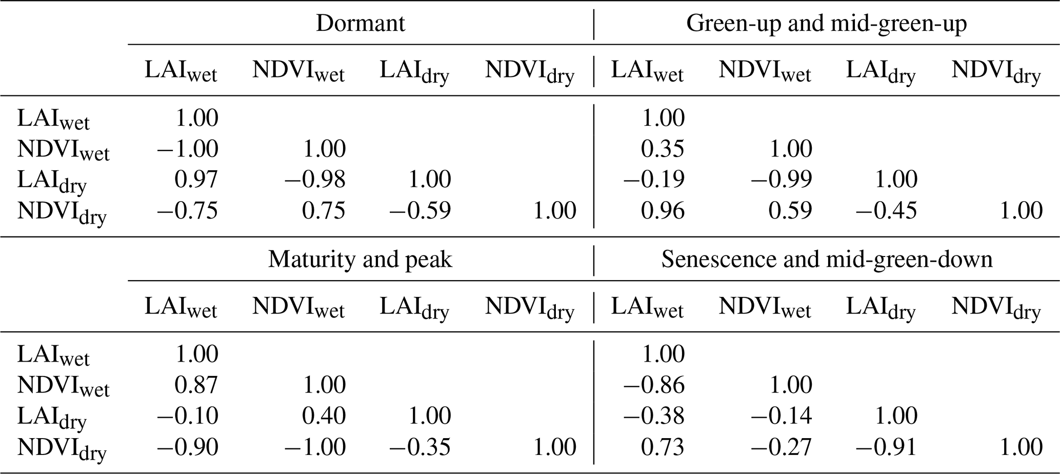
Fuller (1999) observed that in the wet miombo woodland, the co-occurrence of leaf fall and leaf flush in August and September, as shown in Fig. 9, resulted in a net zero change in canopy closure. This net zero change increase in canopy closure may explain the low temporal coefficient of variation in mean LAI values in September (Fig. 8d). The high temporal coefficients of variation in the mean of the aggregated LAI and NDVI values for both the dry and the wet miombo woodland during the maturity and peak phenophase (Fig. 8d) in the mid-rainy season can be attributed to two factors: the heterogeneous growth of the green biomass of the woodland, occurring between January and May (Chidumayo, 2001; Fuller, 1999), and the influence of cloud cover on the quality of satellite-based LAI and NDVI products (Vermote and Wolfe, 2015; Zhang et al., 2003). Furthermore, differences in canopy closure between the dry miombo woodland and the wet miombo woodland (Fuller, 1999) may contribute to variations in the temporal coefficients of variation in the mean of the aggregated LAI and mean NDVI values during the maturity and peak and senescence and green-down phenophases. For example, the dry miombo woodland, which has a lower canopy closure compared to the wet miombo (Fuller, 1999), is likely to have a higher grass component. Additionally, differences in miombo species composition, distribution of rainfall, soil type, and soil moisture, among other variables, may result in varied phenological differences between the dry miombo woodland and the wet miombo woodland (Chidumayo, 2001; Fuller, 1999).

Overall, the results of the ANOVA (see Fig. S10 and Table S2) indicate that there is no significant difference between the means of each satellite-based evaporation estimate for the dry miombo woodland and wet miombo woodland.

3.3 Phenophase-based difference in satellite-based evaporation estimates

3.3.1 Deseasonalised time series, evaporation trend, and evaporation anomalies

The original time series and the deseasonalised time series for the Luangwa Basin miombo woodland, dry miombo woodland, and wet miombo woodland are displayed in Figs. S4 and S5. The temporal monthly anomalies of the means of evaporation, LAI, and NDVI are presented in Fig. 10. The deseasonalised time series exhibits diverse temporal dynamics and magnitudes in satellite-based evaporation estimates for both dry miombo woodland and wet miombo woodland for the period from 2009 to 2020 (Fig. S4). The Mann–Kendall trend analysis reveals different degrees of decline in deseasonalised evaporation estimates by FLEX-Topo, GLEAM, SSEBop, and WaPOR (Kendall's τ > −0.1; p value < 0.05). Conversely, MOD16A2 and TerraClimate demonstrate no discernible trend (refer to Table S3). Overall, the evaporation anomalies, LAI anomalies, and NDVI anomalies (Fig. 10a) suggest that differences in the satellite-based evaporation estimates vary depending on the phenophase with more nuanced temporal variations that are pronounced in the dormant phenophase in the dry season. There also seem to be two peaks in evaporation during the green-up and mid-green-up and maturity and peak phenophases. Similar peaks in LAI and NDVI are also observed during the same periods, which indicates a positive correlation between canopy cover and evaporation. However, this relationship does not seem to hold true during the dormant phenophase in the dry season (Fig. 10). Although the MOD16A2 and TerraClimate estimates show contrasting temporal dynamics and higher evaporation values, the rest of the satellite-based evaporation estimates appear to have a similar temporal pattern during the green-up and mid-green-up and maturity and peak phenophases during the rainy season.

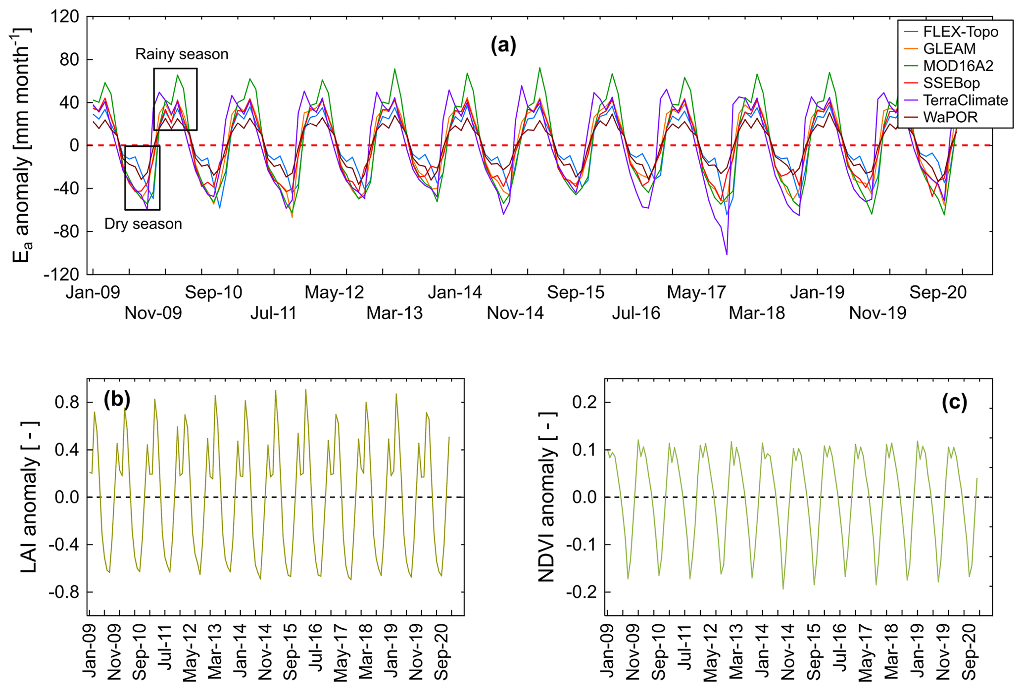
Figure 10 Temporal monthly anomalies of the mean satellite-based evaporation estimates (a), monthly anomalies of mean LAI (b), and monthly anomalies of mean NDVI (c) time series for the miombo woodland in the Luangwa Basin.

These discrepancies in deseasonalised time series, trends, and monthly anomalies reveal the divergent temporal dynamics in satellite-based evaporation estimates in the miombo woodland within the Luangwa Basin. The sections that follow provide detailed analyses of the anomalies and deseasonalised data based on phenophases (which are shown in Fig. 2 and described in Sect. 2.2.1).

3.3.2 Temporal distribution and correlation of satellite-based evaporation estimates

Figure S3 shows the temporal distribution of evaporation in relation to the proxy for woodland canopy cover (i.e. NDVI) and rainfall across phenophases in a hydrological year of the Luangwa Basin. The highest temporal-mean satellite-based evaporation estimates were observed in the maturity and peak phenophase during the rainy season (with the highest NDVI values), while the lowest were in the dormant phenophase in the dry season (with the lowest NDVI values) (Fig. S3). With reference to original time series, deseasonalised time series, and monthly time series of anomalies, in different phenophases, each satellite-based evaporation estimate appeared to correlate differently with other evaporation estimates (Figs. 11, 12, and S6–S9).

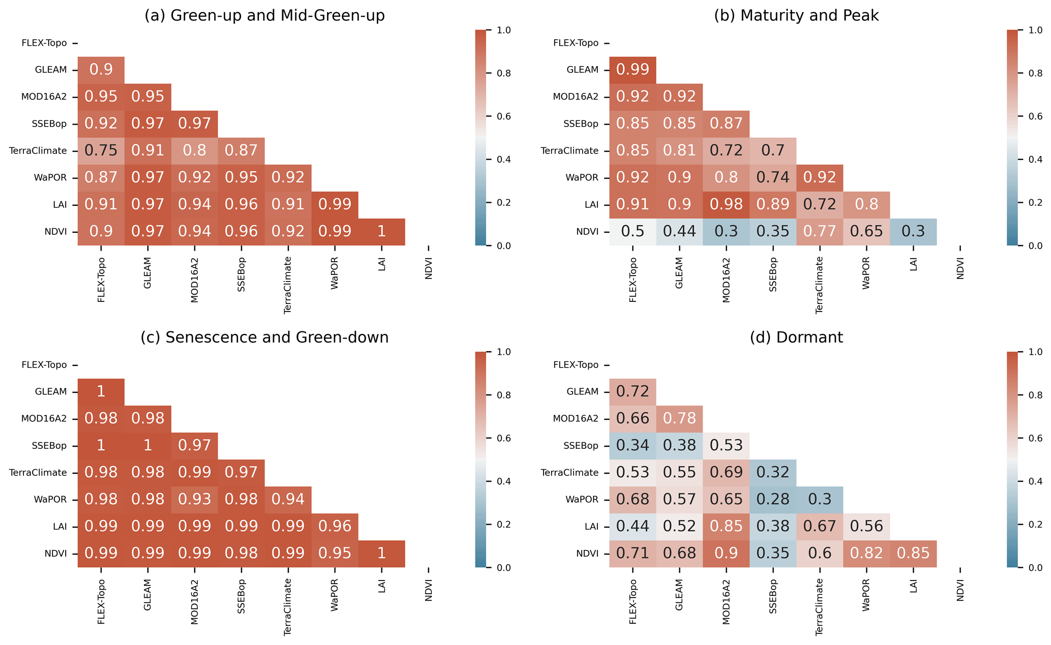
Figure 11 Temporal correlation of monthly anomalies of mean satellite-based evaporation estimates, mean LAI, and mean NDVI in the miombo woodland, Luangwa Basin, Zambia. (a) Green-up and mid-green-up phenophase, (b) maturity and peak phenophase, (c) senescence and green-down phenophase, and (d) dormant phenophase.

A correlation analysis of the means of the temporal time series showed significantly stronger correlation coefficients (r>0.5; p value < 0.05) among the satellite-based evaporation estimates during the transition periods in the green-up and mid-green-up and senescence and mid-green-down phenophases (Figs. 11 and 12). On the contrary, significantly weaker correlations (r<0.5; p value < 0.05) were observed during the dormant phenophase in the warm-dry season (Figs. 11, 12, and S6–S9). Stronger correlations between the temporal satellite-based evaporation estimates appear to occur during periods with high woodland leaf area, high soil moisture content, and high vegetation water during transition periods into the rainy season and into the dry season (Figs. 5, 7, 11, and 12).

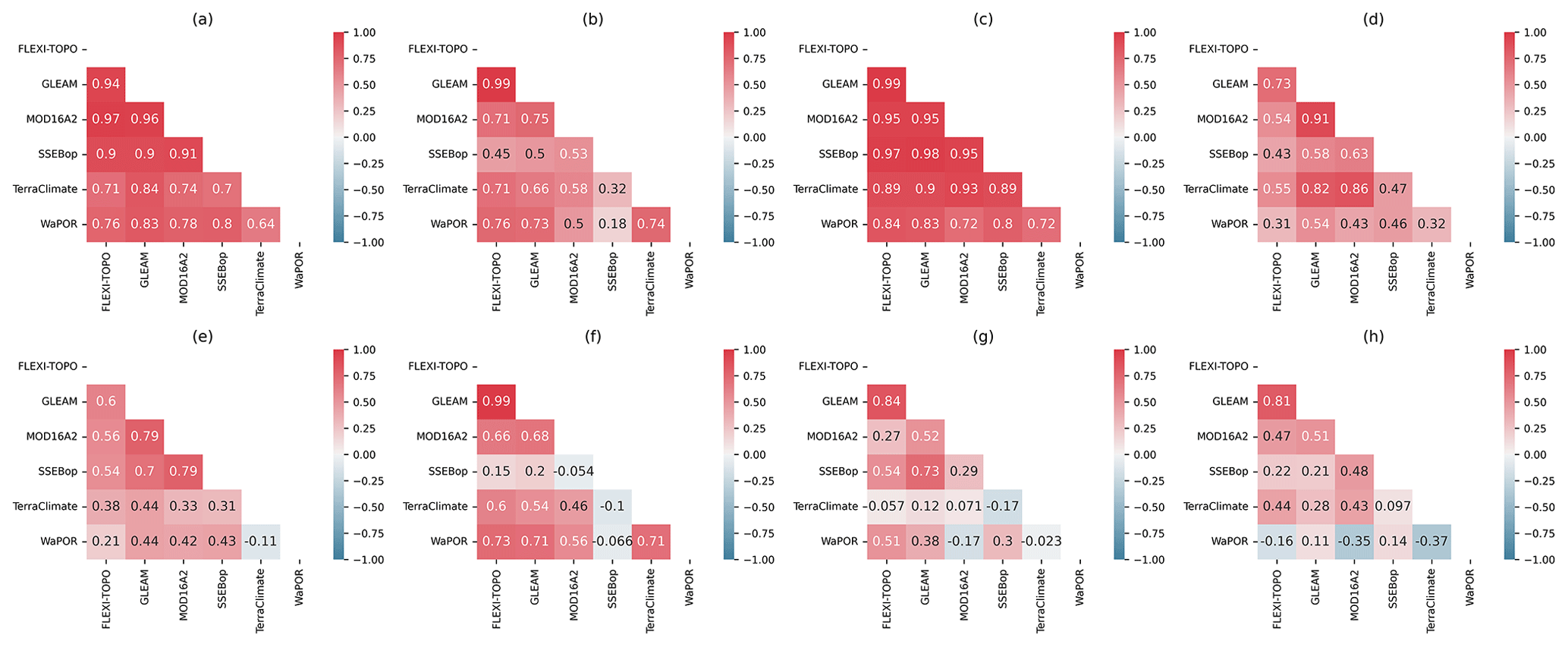
Figure 12 Temporal correlation of the monthly means of satellite-based evaporation estimates and proxies (LAI and NDVI) for woodland canopy cover for the miombo woodland in the Luangwa Basin across satellite-based phenophases: (a–d) original time series, (e–h) deseasonalised time series. (a, e) Green-up and mid-green-up; (b, f) maturity and peak; (c, g) senescence, green-down, and mid-green-down; and (d, h) dormant phenophases.

On the other hand, the lowest temporal correlation coefficients among satellite-based evaporation estimates appear to occur during periods of water stress in the warm-dry season (Figs. 5, 7, 11, 12, and 13). Generally, compared to original time series, the deseasonalised time series yielded lower coefficients of correlation among the satellite-based evaporation estimates across seasons and phenophases (Figs. 12 and 13) and highlighted the significance of deseasonalising and removing trends from time series for a better understanding of real correlations. The same pattern in the temporal correlation of the satellite-based evaporation estimates observed for the miombo woodland at the Luangwa Basin scale was also observed for both the dry miombo woodland and the wet miombo woodland (Figs. S6–S9).

3.3.3 Temporal variations in satellite-based evaporation estimates across phenophases

Original time series and deseasonalised time series of satellite-based evaporation estimates

A comparison of the aggregated means of the satellite-based evaporation estimates from 2009 to 2020 showed that the temporal coefficients of variation (CVs) for the original time series (Fig. 13a–d) were larger, while the CVs for the deseasonalised time series (Fig. 13e–h) were lower between phenophases (see Fig. 13). This finding further emphasises, as mentioned above, the importance of eliminating seasonality and trends from time series when assessing long-term relationships among variables.

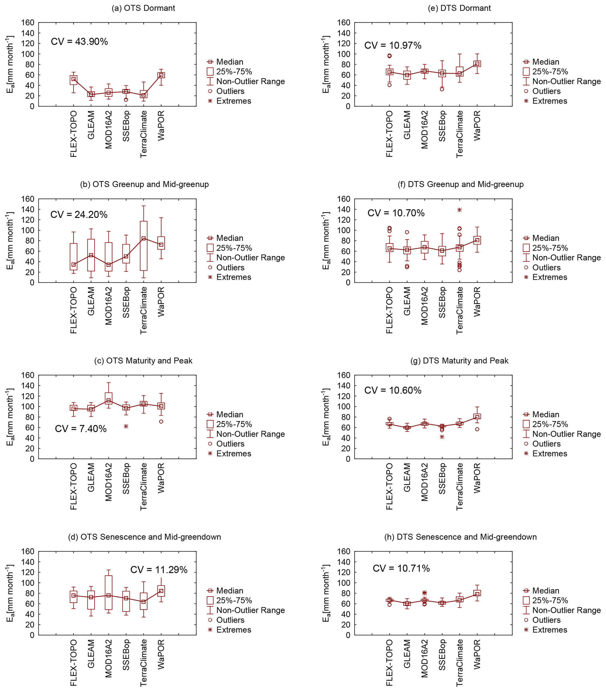
Figure 13 Boxplots comparing satellite-based evaporation estimates, (a–c) original time series (OTS) and (c–f) with deseasonalised time series (DTS), across phenophases of the miombo woodland for the period 2009–2020 in the Luangwa Basin. The temporal coefficient of variation (CV) is for the comparison between the six satellite-based evaporation estimates.

Phenophases and coefficients of variation in satellite-based evaporation estimates

The higher temporal coefficient of variation in the means of satellite-based evaporation estimates – 43.90 % and 10.97 % for original time series (Fig. 13a) and deseasonalised time series (Fig. 13e) respectively – shows that there are significant differences in the amount of evaporation estimates during the dormant phenophase (Figs. 13 and S10). This indicates that the adapted phenological and physiological attributes of the miombo species may play a role in regulating evaporation during the dormant phenophase in the dry season. The CV from the comparisons of the temporal means of satellite-based evaporation estimates increases during this period because it is when the most changes occur in phenology, such as the co-occurrence of leaf fall and leaf flush (i.e. changes in LAI) as well as changes in leaf colour (i.e. changes in NDVI). This is also the driest period of the year, with rising temperatures, during which adapted physiological characteristics, such as accessing groundwater, likely come into play to withstand the dry-season conditions. Therefore, there are differences in how satellite-based estimates account for these changes in climate variables and phenological changes, resulting in the observed high CVs. Additionally, the CVs from the comparison of the monthly estimates for each satellite-based estimate (Table S4) show that CVs are higher in the dormant phenophase, which is probably due to reduced soil moisture and the changes in the woodland canopy as a result of the leaf fall and leaf flush that affects the surface area for evaporation. The green-up and mid-green-up phenophase is a transition phenophase between the dry season and the rainy season. A reduction in the CV to almost half of its value was observed – from 43.90 % in the dormant phenophase to 24.3 % in the green-up and mid-green-up phenophases. The green-up and mid-green-up phenophase is at the start of the rainy season, with an increasing LAI, high canopy cover (i.e. mean NDVI between 0.5 and 0.7), and the highest net radiation (i.e. 150 W m⁻²) (Figs. 5, 7, and 8). The increasing woodland canopy cover (i.e. LAI) and soil water conditions due to rainfall activity probably reduce the uncertainty in evaporation assessment, as can also be evidenced by the increased temporal correlation coefficients between the satellite-based evaporation estimates (Figs. 11a and 12a). In Table S4, the green-up and mid-green-up phenophase showed the largest CVs of satellite-based evaporation estimates. This is probably due to both the continued changes in the woodland canopy cover, which affect the evaporative surface area, and the commencement of rainfall activities, resulting in temporal variations in evaporation (Figs. 5, 7, and 8). The maturity and peak phenophase in the rainy season showed the least CV, 7.40 % for the original time series and 10.60 % for the deseasonalised time series between the satellite-based evaporation estimates. The lower CVs are indicative of a reduction in differences in the means of satellite-based evaporation estimates during periods with high woodland canopy cover and high soil moisture content. Table S4 also shows the lowest CVs of each satellite-based evaporation estimate during the maturity and peak phenophase. This is probably a result of the woodland canopy cover being established and uniform when there is no leaf fall and leaf flush, providing a stable evaporative surface. Additionally, consistent rainfall activity and soil moisture would have been attained by this period, therefore not causing significant variations in the evaporation (Figs. 5, 7, and 8). The senescence and green-down phenophase is a transitional phenophase between the rainy season and dry season. During this phenophase, the differences in the means of satellite-based evaporation are low relative to the dormant phenophase (CV = 11.29 % and 10.71 % for the original time series and deseasonalised time series respectively). However, relative to the maturity and peak phenophase, they indicate the beginning of an increase in differences in the means of satellite-based evaporation estimates. Table S4 show high CVs for each satellite-based estimate relative to the maturity and peak phenophase, as variations in rainfall increase and soil moisture begins to decrease (Figs. 5, 7, and 8).

3.3.4 Satellite-based evaporation estimates and phenology of the miombo woodland in the dry season

In the dormant phenophase in the warm-dry season, WaPOR, followed by FLEX-Topo, showed higher estimates of evaporation compared to other satellite-based evaporation estimates (Figs. 13 and S10 and Table S4). Zimba et al. (2023) showed, at point scale in the wet miombo woodland, that satellite-based evaporation estimates (FLEX-Topo, GLEAM, MOD16, SSEBop, TerraClimate, and WaPOR) underestimated actual evaporation in the warm-dry season. They also showed that while the NDVI was generally on a downward trajectory from May to September, the observed actual evaporation estimates had a rising trajectory, which was in agreement with the rising air temperature and net radiation. Compared to other satellite-based estimates, WaPOR followed the same temporal dynamics as the field observations of actual evaporation in the wet miombo woodland in the dry season (Zimba et al., 2023). In this study, WaPOR showed a negative correlation with the LAI and NDVI in the warm dry season and dormant phenophases (Fig. 12g, h). Therefore, with reference to findings by Zimba et al. (2023) and Fig. 12g, h, WaPOR appears to have the correct temporal dynamics of actual evaporation of the miombo woodland in the cool-dry season and senescence and green-down and the warm-dry season and dormant phenophases.

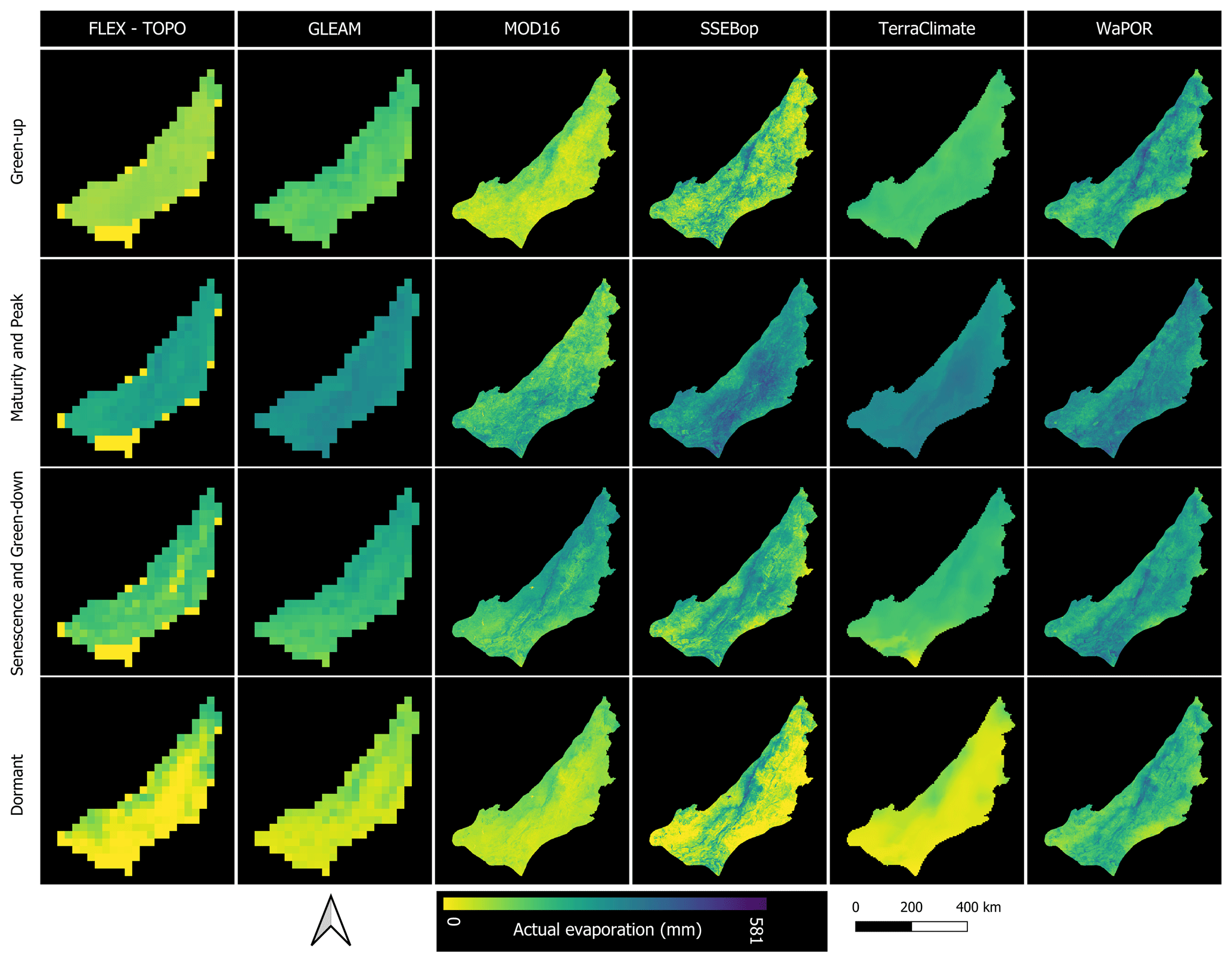
Figure 14 Spatial–temporal distribution of satellite-based evaporation estimates across different vegetation phenophases of the Luangwa Basin for the hydrological year from September 2019–August 2020.

3.3.5 Spatial–temporal distribution of satellite-based evaporation estimates across phenophases

Figure 14 shows the spatial–temporal distribution of satellite-based evaporation estimates across different phenophases for the hydrological year 2019/2020. The comparison was based on the entire Luangwa Basin, including non-miombo-woodland regions. Generally, the spatial distribution and details of evaporation estimates are different, but, like the temporal variations, they are most pronounced in the dormant and green-up phenophases (Figs. 12, 13, and 14 and Table S3). During periods of high soil moisture and high leaf area (i.e. Figs. 5 and 7), in the maturity and peak and senescence and green-down phenophases, the products are more in agreement. It can be further seen that during the dormant phenophase, all six evaporation estimates showed higher actual evaporation in wooded areas (Fig. 14) (refer to Fig. 1b, c for the cover of the miombo woodland in the Luangwa Basin). Potential contributing factors to the observed differences in the spatial–temporal distribution of satellite-based evaporation estimates are highlighted in Sect. 3.5.

3.3.6 Pairwise multiple comparison of satellite-based evaporation estimates at the Luangwa Basin miombo woodland scale

As indicated earlier, there are no statistically significant differences in the mean estimates of evaporation for the dry miombo woodland and wet miombo woodland based on each satellite-based evaporation estimate (Fig. S10 and Table S2). Therefore, all pairwise comparisons were performed only for the entire miombo woodland of the Luangwa Basin. Tables S5 and S6 show the results of all pairwise multiple comparisons of satellite-based evaporation estimates, with seasonality (Table S5) and the deseasonalised time series (Table S6). For each phenophase (i.e. group), 33 monthly estimates (i.e. samples) of evaporation for each satellite-based estimate were used in the comparison. For both time series, it appeared that the WaPOR estimates were the most different across phenophases (Fig. 15). The other satellite-based evaporation estimate with mean estimates that are significantly different from other estimates, after WaPOR, is FLEX-Topo, followed by MOD16 and TerraClimate (Fig. 15; Tables S5 and S6).

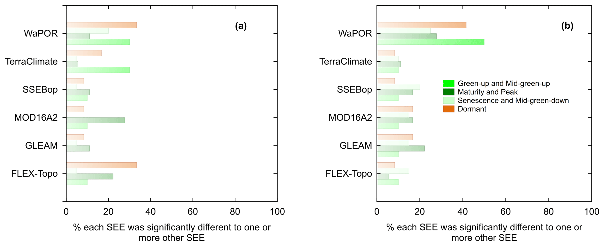
Figure 15 Percentage by which each satellite-based evaporation estimate (SEE) was significantly different to one or more other SEEs in each phenophase at the Luangwa Basin miombo woodland scale. (a) Comparison of satellite-based evaporation estimate original time series (OTS). (b) Comparison of satellite-based evaporation estimate time series with deseasonalised time series (DTS).

3.3.7 Temporal variations in climate-, LAI-, NDVI-, and satellite-based evaporation estimates

With the exception of WaPOR, monthly temporal variations of the comparisons of the monthly means for each satellite-based evaporation estimate were the highest during the green-up phenophase followed by the dormant and senescence and green-down phenophases (Fig. 16). The maturity and peak phenophase showed the lowest temporal coefficients of variations in the monthly means of each satellite-based evaporation estimate (Fig. 16 and Table S4). The green-up and senescence and green-down phenophases are at the boundaries of the dry season and the mid-rainy season (in the case of the green-up phenophase) and the rainy season and the dry season (in the case of the senescence and green-down phenophases). The temporal coefficients of variation in the monthly means of NDVI (i.e. canopy cover), rainfall (i.e. water availability), and temperature (i.e. energy availability) in the green-up and senescence and green-down phenophases (Fig. 16) likely explain the temporal variations in the monthly means of each satellite-based evaporation estimate. The phenophases in which the means of LAI, NDVI, rainfall and soil moisture appear to show higher temporal coefficients of variation are also the phenophases in which the monthly means of individual satellite-based estimates show higher temporal coefficients of variation (Fig. 16). The observed temporal coefficients of variation in the monthly means of each satellite-based evaporation estimate in the dormant phenophase could be a result of the increase or reduction in the canopy cover due to the leaf fall, leaf flush, and leaf colour changes (i.e. NDVI, as shown in Figs. 7, 8, 9, and 15). Figure 16 generally shows that the temporal variations in the means of the LAI, NDVI, rainfall, soil moisture, and air temperature are mirrored by the temporal variations in the means of satellite-based evaporation estimates. As a result, satellite-based evaporation estimates are likely to exhibit significant variations due to weather conditions and year-to-year weather differences.

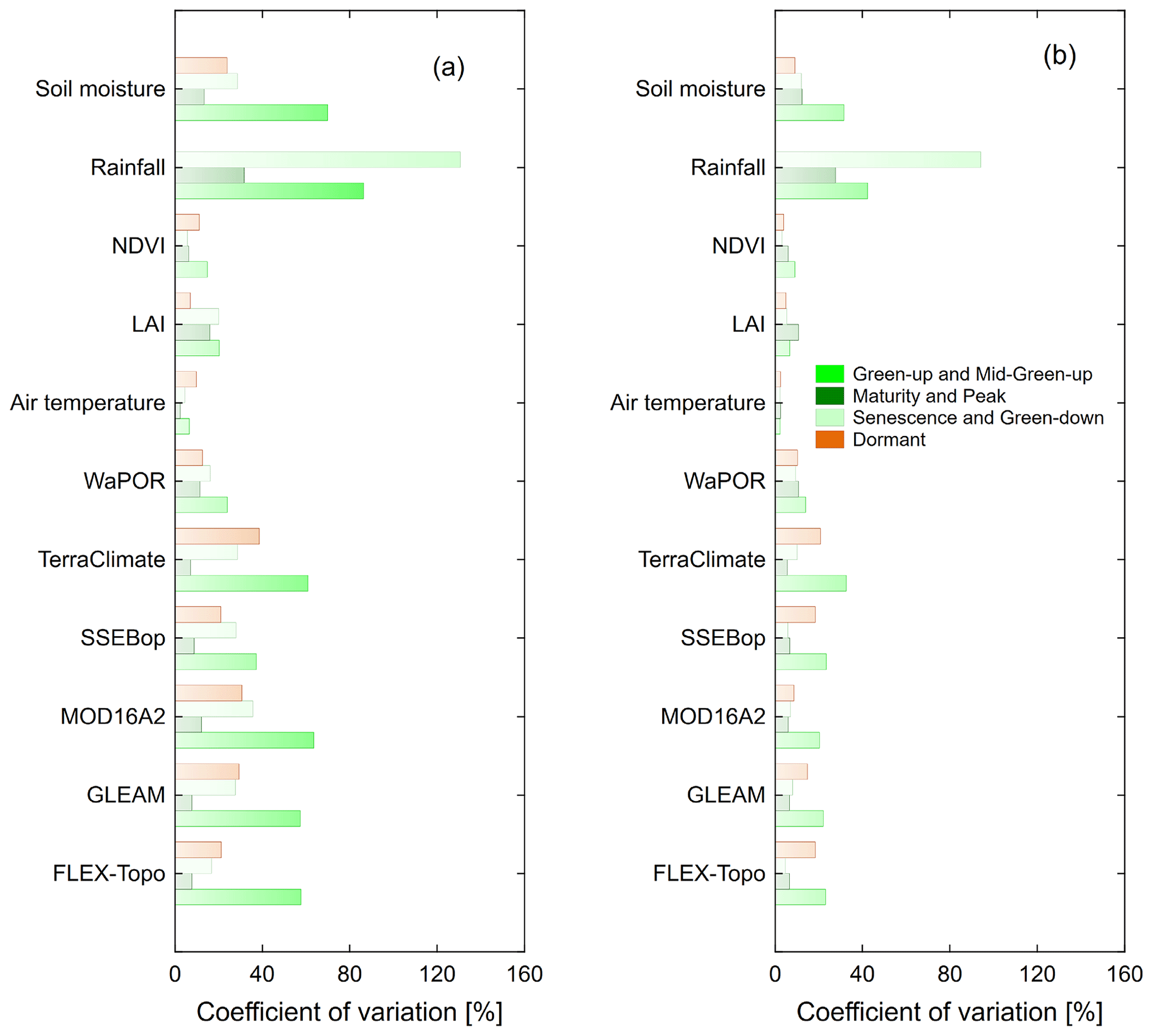
Figure 16 Temporal coefficients of variations in the means of variables for (a) original time series (OTS) and (b) deseasonalised time series (DTS) across phenophases for the miombo woodland, Luangwa Basin.

3.4 Comparison of satellite-based evaporation estimates to the water-balance-based actual evaporation

Figure 17a compares satellite-based evaporation estimates with water-balance-based actual evaporation estimates for the Luangwa Basin during the hydrological years from September 2009 to August 2020. This comparison includes non-miombo-woodland areas. Except for FLEX-Topo (r= 0.55; p value < 0.05), all other satellite-based evaporation estimates showed a weak correlation (r<0.5; p value > 0.05) with the water-balance-based actual evaporation (E_wb) (Fig. S11 and Table S7). Compared to the E_wb estimates, all six satellite-based evaporation estimates underestimated actual evaporation (Fig. 17b). The poor correlation of E_wb with satellite-based evaporation estimates can be the case due to several factors.

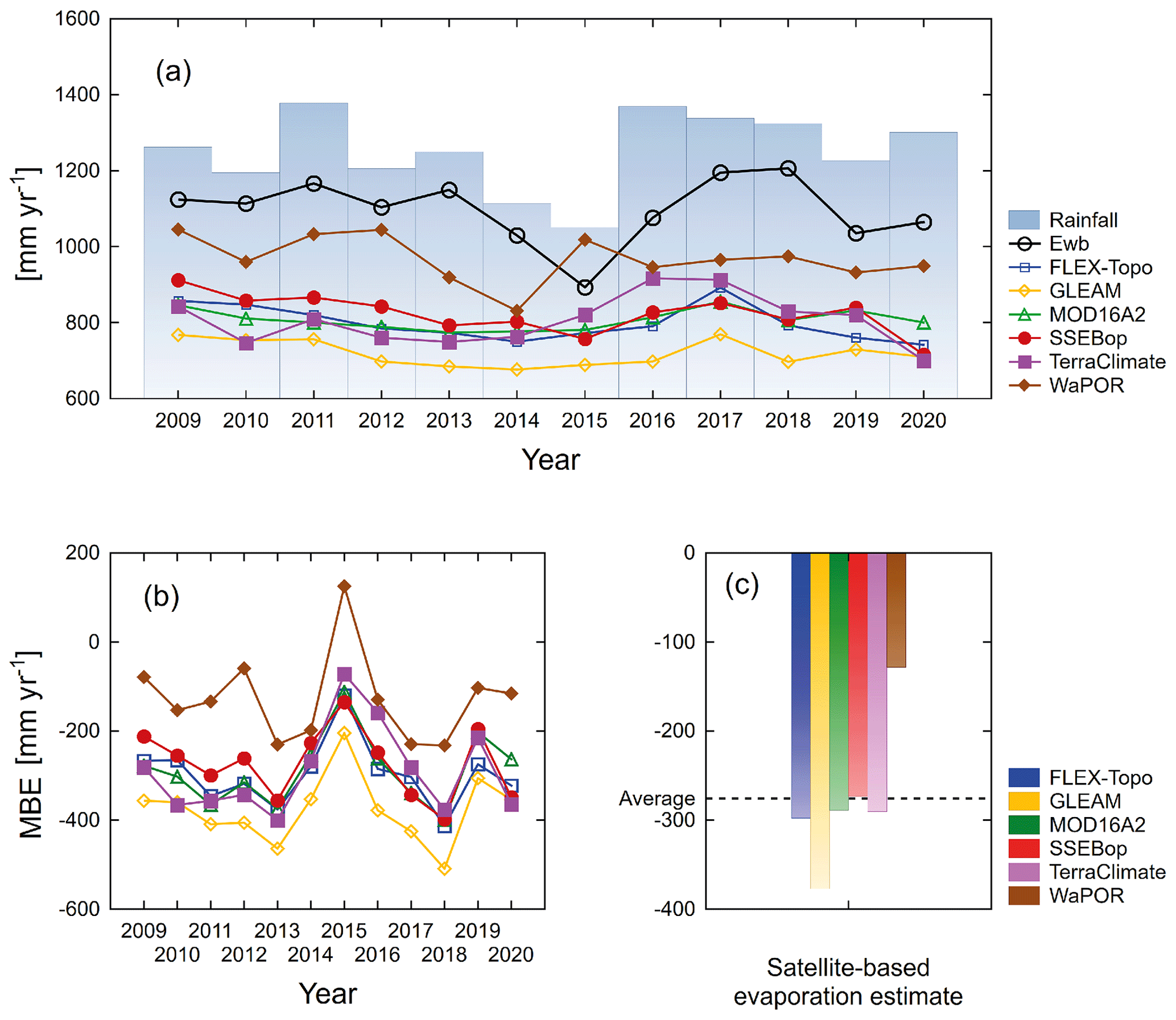
Figure 17 (a) Temporal comparison of satellite-based evaporation estimates to the water-balance-based estimate of actual evaporation for the Luangwa Basin, (b) comparison of the MBE of satellite-based evaporation estimates for each year, and (c) comparison of the multi-year average MBE of individual satellite-based evaporation estimates.

Firstly, the disregard of inter-annual storage may explain the very low actual evaporation estimate in the dry year 2015. In that year, the over-year storage should likely not be disregarded, and it is also possible that farmers in the cropland areas withdrew water from small dams. Taking these factors into account would have led to a higher actual evaporation estimate in 2015. Secondly, the overall higher water-balance-based actual evaporation may be due to the disregard of potential inter-basin groundwater exchange, or leakage of groundwater into the Zambezi. Hulsman et al. (2021) estimated that this leakage could, on average, amount to 143 mm yr⁻¹. This amount would be enough to bridge the bias between WaPOR and the water-balance-based actual evaporation in Fig. 17c.

Furthermore, there are uncertainties in the river discharge and the spatially averaged precipitation, which may have been overestimated. The extended runoff time series with TerraClimate (Fig. 4c, d) may have been overestimated, resulting in underestimating the water-balance-based actual evaporation at the basin scale. The assumption of overestimation of the extended runoff data is based on the validation results of the linear equation used to extend the runoff time series, which showed that RMSE = 27 mm yr⁻¹ and MBE = 21 mm yr⁻¹. In any given year, WaPOR appeared to have the least underestimation, with an average MBE of 120 mm yr⁻¹, while GLEAM had the largest underestimation, with an average MBE of 370 mm yr⁻¹ (Fig. 17c).

At the basin scale, it appeared that there was no statistically significant correlation (r= −0.63; p value = 0.18; α = 0.05) between spatial resolution and evaporation estimates of each product (Fig. 18). For instance, TerraClimate, with a coarser spatial resolution, showed similar bias estimates as SSEBop and MOD16. MOD16 had an even higher spatial resolution than SSEBop, but underestimated more. FLEX-Topo had a coarser spatial resolution than MOD16 and SSEBop but exhibited higher estimates in the warm-dry season in the dormant phenophase (Figs. 14 and S3). The lack of a clear relationship between spatial resolution and actual evaporation estimates (Fig. 18) may imply that other factors, such as the heterogeneity in the land cover (i.e. miombo woodland, mopane woodland, cropland, and settlements); access to soil moisture and groundwater; and differences in model structure (such as the inclusion of leakage), processes, and model inputs, as highlighted in Zimba et al. (2023) and Sect. 3.5 in this study, may be the largest contributing factors to the observed differences in the actual evaporation estimates at the basin scale.

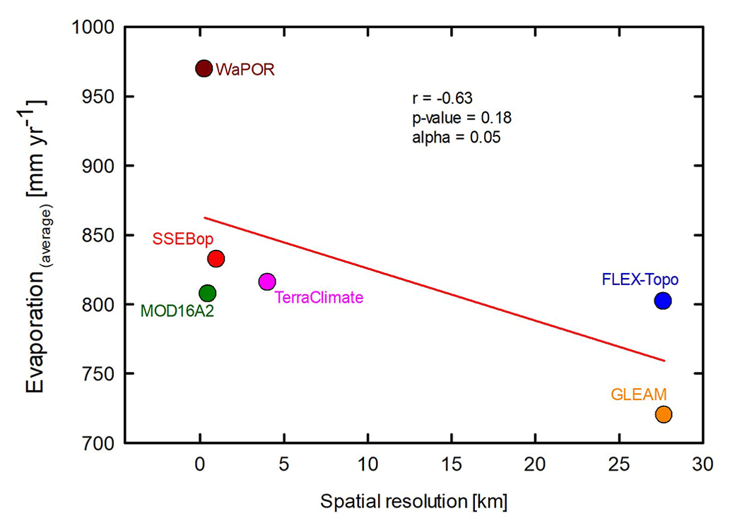
Figure 18 The relationship between 2009 and 2020 annual averages and spatial resolution of satellite-based evaporation estimates at the Luangwa Basin scale.

However, the underestimation of actual evaporation at basin scale by satellite-based evaporation estimates cannot be entirely attributed to the inaccuracies in the simulation of miombo woodland evaporation. The evaporation of other vegetation types, i.e. mopane woodland, has not been investigated. The basin-scale water-balance-based comparison suggests that satellite-based evaporation estimates possibly underestimate actual evaporation in non-miombo-woodland landscapes as well. This requires further investigation of different landscapes and land covers such as grassland, shrubland, wetland, and mopane woodland. For a more comprehensive understanding of the evaporation in the Luangwa Basin, there is a need for the assessment of the interactions between plant phenology and climate of each vegetation type and the accompanying potential influence on the evaporation dynamics in the basin. Nevertheless, the results of this study agreed with Weerasinghe et al. (2020b), who showed that most satellite-based evaporation estimates generally underestimate evaporation across African basins (i.e. the Zambezi Basin). The lower underestimation by WaPOR agreed with the point-scale field observations for the wet miombo woodland (Zimba et al., 2023) and suggests that WaPOR is the closest to actual evaporation of the miombo woodland in the Luangwa Basin.

3.5 Potential causes of differences in trends, magnitudes, and spatial distribution of satellite-based evaporation estimates

Most pronounced differences in temporal dynamics and magnitudes of satellite-based evaporation estimates of the miombo woodland have been observed in the dormant phenophase of the dry season (Figs. 11–15 and Table S3). Evaporation during that period is dominated by transpiration (e.g. Tian et al., 2018). The dominant phenological characteristic of the miombo species in the dry season is the co-occurrence of leaf fall, leaf flush, and green-up before the commencement of seasonal rainfall (Figs. 7 and 9; Chidumayo and Frost, 1996; Frost, 1996), which affects transpiration (e.g. Marchesini et al., 2015; Snyder and Spano, 2013). Tian et al. (2018) showed that the terrestrial groundwater storage (TGS) anomaly continued to decrease throughout the dry season and was indicative of the fact that miombo trees used deep groundwater during that period. The suggestion that miombo trees access groundwater is supported by Savory (1963), who showed that miombo species are deep-rooting beyond 5 m in depth, with the capacity to access groundwater. Therefore, it is likely that satellite-based evaporation estimates using models whose structure, processes, and inputs take into account the highlighted interactions between plant phenology and climate during the dry season and early rainy season, especially the access to deep soil moisture, would produce more accurate trends and magnitudes of evaporation in the miombo woodland.

3.5.1 Use of proxies for soil moisture

Some studies have shown that direct integration of soil moisture rather than the use of proxies improves the accuracy of actual evaporation estimates (Brust et al., 2021; Novick et al., 2016). The challenge when using proxies for soil moisture – for example, in surface energy balance models – is that these are unable to fully account for changes in other factors that may influence sensible heat fluxes (Gokmen et al., 2012). To improve the accuracy of the estimation of water and energy fluxes in regions with recurrent plant water stress, such as in miombo woodland, Gokmen et al. (2012) suggested that the soil moisture be integrated in surface energy-balance models. For instance, for MOD16, the use of the relative humidity and vapour pressure difference as proxies for soil moisture may be a source of uncertainty in estimating transpiration (Novick et al., 2016). Direct integration of soil moisture into the MOD16 algorithm appeared to improve the accuracy of actual evaporation estimates (Brust et al., 2021). The energy balance-based SSEBop does not explicitly consider soil moisture dependency and assumes that the variations in satellite-based land surface temperature and vegetation indices, such as the NDVI, account for soil moisture (Senay et al., 2013). TerraClimate uses the plant-extractable water capacity of soil for soil moisture input. However, the difficulty in determining the plant-extractable water capacity of the soil is in defining the extent of the rooting depth. GLEAM takes into account 2.5 m of the sub-surface linked to observed precipitation. On the other hand, transpiration in FLEX-Topo and WaPOR (ETLook model) is coupled with soil moisture in the root zone using an integrated approach. Consequently, this may explain why the pairwise comparison showed that trends and magnitudes of FLEX-Topo and WaPOR were not significantly (p value > 0.05) different (in both dry miombo woodland and wet miombo woodland) during the dormant phenophase (Table S5d). Therefore, the integration of soil moisture into evaporation simulations and the accuracy of the soil moisture product used are likely to affect the accuracy of satellite-based transpiration estimates.

3.5.2 Optimisation of the rooting depth

Optimising rooting depth rather than using a standard depth has been shown to increase transpiration of trees in landscapes with a dry season (Kleidon and Heimann, 1998). Modifying rooting depth can improve energy flux simulations at both the field scale and the regional scale (Liu et al., 2020). Wang-Erlandsson et al. (2016) showed that accurate root zone storage estimates “improved evaporation simulation overall, and in particular during the least evaporating months in sub-humid to humid regions with moderate to high seasonality”. Their study demonstrated that several forest types have developed root zone storage mechanisms that help buffer for dry-season conditions. Some miombo species are deep-rooting beyond 5 m in depth, while the soil moisture in the miombo woodland increases with depth (i.e. Chidumayo, 2001; Savory, 1963). Additionally, the depth to groundwater ranges between 0 and 25 m b.g.l. for both wet miombo woodland and dry miombo woodland, although, in a few places, the range is between 25 and 50 m b.g.l. (Bonsor and Macdonald, 2011). Therefore, one of the potential causes of the observed differences in satellite-based evaporation estimates could be the rooting depth used in the simulation of evaporation. The satellite-based evaporation estimates used in this study are likely not to have optimised rooting depth for the miombo woodland as there are few studies in the public domain that have conducted field-based investigations to determine the optimum rooting depth for effective simulation of transpiration of miombo woodland. Since ecosystems have adapted to local climatic conditions (Tian et al., 2018), global-scale root storage estimates and optimisation may not be able to effectively capture the climatic conditions at the local and regional scales.

3.5.3 Differences in land cover products used

The land cover proxies in satellite-based evaporation estimates may also explain the observed differences in both temporal and spatial distributions of evaporation. For instance, MOD16 uses a global land cover product (Gray et al., 2019), which was shown to misclassify certain land cover types and to have low user accuracy in certain regions (i.e. Leroux et al., 2014). WaPOR uses the Copernicus Land Cover product but adds the distinction between irrigated and rain-fed areas (FAO, 2020). For the vegetation fraction, GLEAM uses MODIS MOD44B (Martens et al., 2017; Miralles et al., 2011). Other satellite-based evaporation estimates (i.e. SSEBop) use vegetation indices, such as the NDVI, as a proxy for vegetation cover.

Different vegetation types have different interactions between plant phenology and climate (i.e. Lu et al., 2006), which influences actual evaporation (Forster et al., 2022; Snyder and Spano, 2013; Schwartz, 2013). Transpiration of the miombo woodland in the dry season is dependent on the land cover type and constrained by root zone water availability (Wang-Erlandsson et al., 2016; Gates and Hanks, 2015; Stancalie and Nert, 2012; Allen et al., 1998), stomatal conductance thresholds, and surface roughness, which are dependent on vegetation type and plant species (Urban et al., 2017; Wehr et al., 2017; Gates and Hanks, 2015; Tuzet, 2011). Therefore, dissimilarities in the land cover products and their associated limitations are possibly reflected in differences in the spatial–temporal distribution of satellite-based evaporation estimates.

3.5.4 Satellite-based rainfall products and rainfall interception

The differences observed in evaporation estimates may be related to differences in the quality of satellite-based precipitation products used and the ability of the models to effectively account for rainfall interception. Studies have shown that satellite precipitation products are geographically biased towards either underestimation or overestimation (Macharia et al., 2022; Asadullah et al., 2008). In the case of Africa, and southern Africa in particular, no single precipitation product has been found to perform better than other precipitation products across landscapes (Macharia et al., 2022). The difference in precipitation products, with different spatial resolutions and accuracy levels, may explain the differences in the spatial–temporal distribution of satellite-based evaporation estimates during the rainy season. For instance, FLEX-Topo used the Climate Hazards Group Infra-Red Precipitation with Station (CHIRPS) data (Funk et al., 2015a, b), GLEAM used Multi-Source Weighted-Ensemble Precipitation (MSWEP) (Beck et al., 2017), which uses different algorithms, inputs, and spatial resolutions. Rainfall interception is a function of vegetation cover, leaf area index (LAI), spatial scale, and precipitation. For instance, LAI influences canopy interception, throughfall, and forest-floor interception, and spatial and temporal scales influence the interception threshold (FAO, 2020; Gerrits, 2010; Savenije, 2004). Field observations showed that wet miombo woodland canopies intercepted up to 18 %–20 % of rainfall annually (i.e. Alexandre, 1977). Therefore, differences in the quality and accuracy of land cover products and even proxies, such as the NDVI, used for modelling interception, are likely to result in different evaporation estimates of evaporation products that have interception modules (i.e. FLEX-Topo, GLEAM, MOD16, and WaPOR).

4 Conclusions and recommendations

This study sought to find out to which extent a variety of satellite-based evaporation estimates were in agreement or differed in quantifying miombo woodland evaporation during its typical phenophases and to establish the underlying factor(s) for the discrepancies that emerged. The study also compared the different satellite-based evaporation estimates to the annual water-balance-based evaporation at the basin scale. The following were the conclusions.

• a.

  Compared to the observed temporal dynamics in canopy display attributes of the wet miombo woodland in the dormant phenophase and the green-up and mid-green-up phenophases in the dry season – i.e. increase in leaf area (i.e. LAI) and the start in green-up (i.e. NDVI) in late September – only WaPOR appeared to follow the field observations of the changes in the plant phenology. Consequently, WaPOR showed higher means of the aggregated estimates of evaporation than the other satellite-based evaporation estimates in the phenophases in the dry season.

• b.

  The original time series, the deseasonalised time series, and the time series of anomalies appeared to show weaker temporal correlation coefficients and high temporal coefficients of variation in the means of aggregated satellite-based evaporation estimates in the dormant phenophase in the dry season. The observed differences in satellite-based evaporation estimates in the dormant phenophase in the dry season appear to be due to the limited understanding and inadequate representation of the interactions between plant phenology and climate that are influenced by the adapted physiological attributes, such as the co-occurrence of leaf fall and leaf flush and the deep-rooting of the miombo species, with potential access to deep soil moisture, including groundwater.

• c.

  It is possible that the underestimations of satellite-based evaporation estimates when compared to the water-balance-based evaporation estimates are affected by the disregard of over-year storage in the deeper groundwater and the export of groundwater by leakage to the downstream Zambezi River. Another cause for the discrepancy is the inadequate representation of the plant phenology and climate interactions of not only the miombo species, but also other vegetation types, such as the mopane woodland. Consequently, field observations of evaporation across the different phenophases and strata of the miombo woodland are required to obtain a comprehensive overview of the characteristics of the actual evaporation of the ecosystem. This information can be used to help improve satellite-based evaporation assessments in the Luangwa Basin and the miombo region as a whole.

• d.

  Finally, in view of the unique plant phenology, whereby the green-up and increase in the leaf area start before the onset of rainfall, and the ability of the miombo species to access additional moisture stocks, inclusion of these traits is likely to improve satellite-based estimates of transpiration of the miombo woodland in the phenophases in the dry season.