Data-driven estimates for the geostatistical characterization of subsurface hydraulic properties

The geostatistical characterization of the subsurface is confronted with the double challenge of large uncertainties and high exploration costs. Making use of all available data sources is consequently very important. Bayesian inference is able to mitigate uncertainties in such a data-scarce context by drawing on available background information in the form of a prior distribution. To make such a prior distribution transparent and objective, it should be calibrated against a data set containing estimates of the target variable from available sites. In this study, we provide a collection of covariance and/or variogram functions of the subsurface hydraulic parameters from a large number of sites. We analyze this data set by fitting a number of widely used variogram model functions and show how they can be used to derive prior distributions of the parameters of said functions. In addition, we discuss a number of conclusions that can be drawn for our analysis and possible uses for the data set.

1 Introduction

Due to high exploration costs, the field of subsurface hydrology is characterized by scarcity of data, leading to high uncertainty (Heße et al., 2019). Collecting data and making them available to practitioners should, therefore, be a high priority. In the field of subsurface hydrology, the largest databases are the World Wide Hydrogeological Parameters DAtabase (WWHYPDA) (Comunian and Renard, 2009) for aquifer sites as well as the SoilKsatDB for soils (Gupta et al., 2021). These databases were launched in 2006 and 2021 with the aim of creating a collaborative catalog of values and statistical distributions needed for subsurface hydrological modeling. The data are stored together with metadata like estimated measurement errors, number of metadata on the site, the measurement technique, length scale, and rock or soil type.

As such, they can serve as a repository for background information that practitioners can draw on to improve their understanding and modeling of the subsurface. Bayesian inference is known for being able to incorporate such background information by virtue of the prior distribution and, therefore, provide information for free. While the role of priors and their choice in statistical inference used to be strongly debated, it is now widely acknowledged that priors that are based on transparent, impartial and observable base rates, i.e., frequencies of the variable in question, provide an objective source of information (Billot et al., 2005; Gilboa et al., 2010; Gelman and Hennig, 2015). In a data-scarce context such as subsurface hydrology, the ability to access such a free source of information is an invaluable asset that has not yet been fully exploited (Heße et al., 2019). Recently, Cucchi et al. (2019) developed and introduced a Bayesian hierarchical model that addresses parts of this challenge. Using this model, it is possible to derive prior distributions for one-point statistics like mean and variance (Heße et al., 2021). One of the biggest challenges, however, is the persistent lack of data on higher-order statistics that would make it possible to derive prior distributions for models describing spatial correlations such as the covariance or (semi-)variogram function. Examples of such statistics are the horizontal and vertical correlation and/or integral scales, anisotropy ratios and variogram/covariance models. As a result, there are no freely available tools that systematically provide background information on such variables. This means that even a simple structural model for spatial heterogeneity, like a Gaussian process (Gelfand and Schliep, 2016), is currently lacking objective and informative prior distributions for its main parameters. For this purpose, it is necessary to collect and analyze a sufficiently large data set suitable for statistical analysis, with the help of which the prior distributions of such multivariate parameters can be determined.

For the collection of these data, different sources are available: primary data in the form of geo-referenced point measurements, secondary data in the form of empirical variogram functions and tertiary data in the form of statistical estimates of subsurface properties. As regards primary data, the SoilKsatDB database provides some geo-referenced measurements, while the WWHYPDA unfortunately does not. In addition, the research literature provides a substantial yet disorganized repository on such data (Bjerg et al., 1992; Rehfeldt et al., 1992; Hess et al., 1992; Welhan and Reed, 1997; Vereecken et al., 2000), primarily for conductivity and transmissivity fields. As regards secondary data, a large number of empirical variogram clouds can be found in the literature. In fact, they provided the majority of estimates on higher-order statistics for our study (see below). In addition, some sources provide curated collections of tertiary data in the form of subsurface statistics, which can be used directly (Jim Yeh, 1992; Gelhar, 1993; Kupfersberger and Deutsch, 1999; Rubin, 2003).

Apart from its above mentioned value for Bayesian inference, a large data set of spatial correlations can be important for a wide range of applications and investigations. First, geostatistical subsurface parameters like the characteristic length scale (Neuman, 1990; Rovey II and Cherkauer, 1995; Sanchez-Vila et al., 1996; Schulze-Makuch et al., 1999; Bromley et al., 2004) or the dispersion coefficient (Pickens and Grisak, 1981; Arya et al., 1988; Cirpka and Kitanidis, 2000; Dentz et al., 2011; Ross et al., 2019) are widely known to show scale effects. This effect is such that their estimated value increases with the observation scale. This observed effect is used to argue that the subsurface should be characterized as a fractal medium (Neuman et al., 2008). Yet so far, this scale dependency has mostly been investigated theoretically or using small data sets (Zech et al., 2015). With a data set like the one provided here, the community of subsurface geostatistics has an empirical basis to investigate this question in more detail.

Furthermore, the data set can be used to compare different established variogram models by, for example, investigating how they differ in parameter estimation with respect to, say, the length scale or the nugget effect. Furthermore, some variogram models have additional shape parameters. A large data set can be used to determine how such added complexity can help to better describe empirical variogram functions and whether the added complexity is justified by greater accuracy in modeling.

Even outside of Bayesian parameter estimation, a data-driven approach like ours can be of use for classic parameter estimation. Virtually all geostatistical software tools provide the ability to apply user-specified initial values. Having good initial values can be key in any optimization routine, and our results can provide such estimates.

Finally, the data set provided here can be used as an empirical basis for a wide range of investigations into the properties and characteristics of subsurface quantities like hydraulic conductivity. Such additional studies can, e.g., investigate under which circumstances any given variogram model function is the best choice and whether there is any connection between a given property of the experimental variogram and some other property of the underlying medium. It can be used to test the applicability of a new variogram model, to test new hypotheses regarding subsurface behavior or to investigate whether cross-correlations between different parameters exist.

In order to outline how we addressed the above objectives, the rest of this paper is structured as follows: we first present the methods used in this study to obtain our results. This includes the sources for our data set and how we compiled them, the covariance/variogram models we used to analyze these data, the software tools and workflows we used, and the online repositories where all data and software solutions can be accessed. This is followed by the Results section, where we present and analyze the statistical properties of the different variogram parameters and show how they can be used to improve the characterization of the subsurface. Furthermore, we critically evaluate the limitations of our study and discuss dangers of misuse. In the final section, Conclusions, we summarize our main findings and show how practitioners can benefit from them.

2 Methods

Let us first look at the tools and methods we used in this study to draw our conclusions. These include the subsurface variogram data sets, the variogram models we used to analyze these data and the numerical tools used for the analyses.

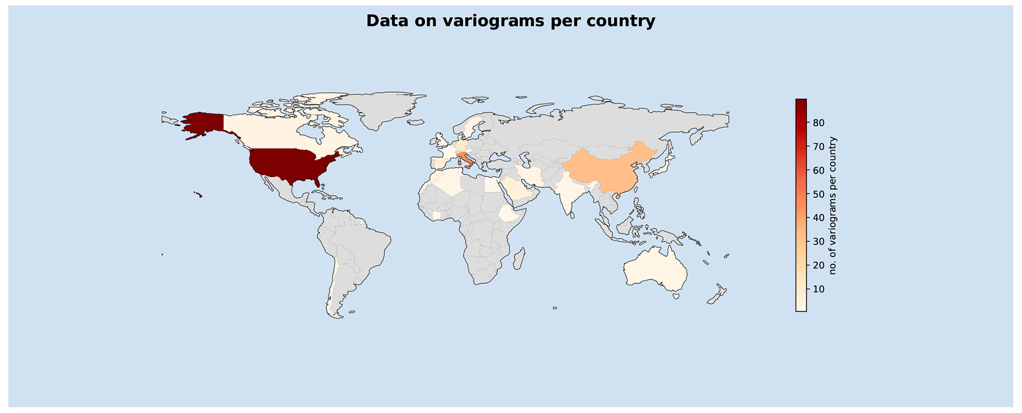
Figure 1 Overview of the countries from where data sets were available.

2.1 Data set

2.1.1 Data sources

To obtain a representative data set of subsurface variogram functions, we conducted a literature search on the ISI Web of Knowledge (https://clarivate.com/webofsciencegroup/solutions/web-of-science/, last access: 31 August 2022). We searched for these data by using the phrases “hydraulic conductivity”, “saturated hydraulic conductivity”, “hydraulic transmissivity”, “hydraulic permeability”, “correlation length”, “spatial variability”, “variogram”, “semi-variogram”, “kriging” and “covariance”. We looked at all the references that came up from this search. If they contained subsurface measurements or a geostatistical analysis of them, we added them to the data set. If reference was made to available data, we tried to contact the corresponding author(s) of the study. The data collected can be divided into three main categories, namely (i) existing data on hydraulic conductivity, transmissivity or permeability (in the form of tables) published in peer-reviewed papers; (ii) processed data on variogram functions in the form of empirical variogram functions derived from the logarithm of these values; and (iii) collections of estimated variogram parameters. It is clear that the first form of data is the most useful as it contains little additional processing, while the last form represents the least amount of information. Overall, however, the second form of data was the most common.

Figure 1 shows a world map of countries where data sets could be collected. The color map shows how many data points are available in each country, while the countries without data are shown in grey. As can be seen, the focus is on North America and western Europe, as is usual for scientific data. But other world regions are also covered to a reasonable extent. So the data set contains a wide range of climate regions and geographical media.

2.1.2 Preparation of the data

Depending on the type of data, we used a number of different workflows to process them. Raw data of hydraulic conductivity, transmissivity and permeability were processed by deriving the empirical variogram cloud from their logarithm, which was subsequently joined with the ones derived from the literature. The empirical variogram clouds found in the literature were available as scatter plots. They were digitized using the freely available WebPlotDigitizer version 4.6 (Rohatgi, 2022). All empirical variogram clouds were then fitted to one of a number of variogram model functions. These model functions and the workflow will be explained below. The last type of data was processed statistics provided in scientific papers of textbooks. To avoid any overlap, we made sure that these statistics were not derived from sites which were already present in the other data. For all data derived from the literature we provide the online sources from where they were taken, by virtue of their digital object identifier in the data file (see below).

2.1.3 Representation of the data

All the data used for this study are made available online in a number of .csv files. In this section, we are going to describe the keywords of these data files.

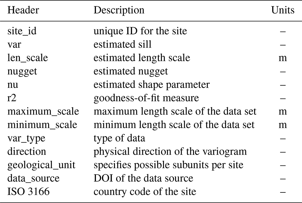
These keywords are depicted in Table 1. The first one is site_id, which provides a unique identifier for the site from which the data were drawn. This name is always based on the name used by the authors which collected the data. The next keywords all refer to estimated variogram parameters. These are var, len_scale, nugget and nu for the variance, length scale, nugget and shape parameter, respectively. The shape parameter is not found in all investigated variogram models. In those cases, the entry is empty. The keyword r2 is the goodness-of-fit measure, i.e., a measure describing how well a given optimum fit of a variogram model function actually fits an empirical variogram cloud. The keywords maximum_scale and minimum_scale describe the maximum and minimum length scale assumed to be present in the data set. In this study, these length scales are interpreted to represent the largest and smallest distances in the data set. The keyword var_type describes the type of variable. In this study, the data can refer to hydraulic conductivity, saturated hydraulic conductivity (for soils), hydraulic transmissivity, hydraulic permeability and indicator variograms of hydraulic conductivity. The keyword direction describes the direction in which the variogram was taken. Direction x is the default direction. This means that it was used in cases where a unidirectional variogram was analyzed, and it was used as the main direction when two horizontal directions were present in the collected data. If two horizontal directions are present, the second direction is always encoded as y . Both x and y therefore have no further physical meaning beyond that. The direction z is always used for the vertical direction. The keyword geological_unit is used in those situations where several variograms are presented in a source for a given site. This situation can represent a number of different situations. In some cases, the authors of the study separated the data by different geologic strata; in some cases, the separation represented geologic subunits that were subdivided by the authors according to their expertise; in some cases, the data represented several actually distinct sites that were combined into a single measurement campaign; and in some cases, it was not clear what criterion was used to make the separation. This keyword may, therefore, represent a number of different situations. The keyword data_source contains the digital object identifier (DOI) to the online resources from which the data were drawn. Finally, the keyword ISO 3166 contains the country code for the country where the data were collected.

Table 1 Name, description and units of the key variables used in the results data file.

2.2 Variogram models

In this study, we used the GSTools Python package (Müller et al., 2022) for the analysis of the empirical data and the covariance models implemented in this package. The data were analyzed with several different model functions, namely the exponential function, the spherical function, the Gaussian function, the Matérn function, the stable function and the truncated power law (TPL) function using Gaussian modes. However, in the vast majority of studies, the spatial heterogeneity in the subsurface is expressed using the (semi-)variogram function γ(h), which is related to the correlation function ρ(h) through the following relationship:

$$\begin{array}{}\text{(1)}& \mathit{\gamma }\left(h\right)=n+{\mathit{\sigma }}^{\mathrm{2}}(\mathrm{1}-\mathit{\rho }(h\left)\right).\end{array}$$

Here we follow the notation of GSTools, described in Müller et al. (2022), where σ² is the correlated variability (or partial sill), meaning the portion of the sill above the nugget n (the uncorrelated variability). The resulting sill or total variance is then the sum of both $s={\mathit{\sigma }}^{\mathrm{2}}+n$. The parameter h is the lag, i.e., the distance between two observation points. The equation above defines an omnidirectional scalar variogram for the sake of brevity. To account for anisotropy and rotation, we refer to Müller et al. (2022), where h is the isotropic distance that is a scalar value and where the distances h_i along the main axis of correlation are incorporated and re-scaled with the respective anisotropy ratios e_i as follows:

$$\begin{array}{}\text{(2)}& h=\sqrt{\sum _{i=\mathrm{1}}^d{\left({\displaystyle \frac{h_i}{e_i}}\right)}^{\mathrm{2}}}.\end{array}$$

Closely related is the covariance function $C\left(h\right)=s-\mathit{\gamma }\left(h\right)$, which is also well known. Such a transformation is possible for all considered variogram/covariance models since they all represent weakly stationary (spatial) processes, meaning that their variance is finite.

The first model function on the list is the exponential model (Webster and Oliver, 2007), which is defined as

$$\begin{array}{}\text{(3)}& \mathit{\gamma }\left(h\right)=n+{\mathit{\sigma }}^{\mathrm{2}}\left(\mathrm{1}-\exp \left(-{\displaystyle \frac{h}{\mathrm{\ell }}}\right)\right),\end{array}$$

with ℓ being the characteristic length scale. Next is the spherical model (Webster and Oliver, 2007), which is defined as

$$\begin{array}{}\text{(4)}& \mathit{\gamma }\left(h\right)=\left\{\begin{array}{ll}n+{\mathit{\sigma }}^{\mathrm{2}}\left(\frac{\mathrm{3}}{\mathrm{2}}\frac{h}{\mathrm{\ell }}-\frac{\mathrm{1}}{\mathrm{2}}\frac{h^{\mathrm{3}}}{{\mathrm{\ell }}^{\mathrm{3}}}\right)& h\le \mathrm{\ell },\\ n+{\mathit{\sigma }}^{\mathrm{2}}& h>\mathrm{\ell }\end{array}\right..\end{array}$$

The next variogram model considered here is the Gaussian model function (Webster and Oliver, 2007). It is defined as

$$\begin{array}{}\text{(5)}& \mathit{\gamma }\left(h\right)=n+{\mathit{\sigma }}^{\mathrm{2}}\left(\mathrm{1}-\exp \left(-{\displaystyle \frac{h^{\mathrm{2}}}{{\mathrm{\ell }}^{\mathrm{2}}}}\right)\right),\end{array}$$

with the parameters having the same definition as above.

These first three model functions are widely used. For example, they represent the vast majority of model functions used in the literature that we used to collect our data set. They also all contain the same number of parameters having the same interpretation. In addition, we also examined three other model functions, all of which contain an additional parameter. The first one is the Matérn function (Rasmussen and Williams, 2005), which is defined as

$$\begin{array}{}\text{(6)}& \mathit{\gamma }\left(h\right)=n+{\mathit{\sigma }}^{\mathrm{2}}\left(\mathrm{1}-{\displaystyle \frac{{\mathrm{2}}^{\mathrm{1}-\mathit{\nu }}}{\mathrm{\Gamma }\left(\mathit{\nu }\right)}}\cdot {\left(\sqrt{\mathit{\nu }}\cdot h\right)}^{\mathit{\nu }}\cdot K_{\mathit{\nu }}\left(\sqrt{\mathit{\nu }}\cdot h\right)\right).\end{array}$$

Here, Γ is the Gamma function, and K_ν is the modified Bessel function of the second kind (Abramowitz and Stegun, 1972). The ν parameter sets the Matérn function apart from the above model functions by introducing an additional degree of freedom and therefore more flexibility in modeling the variogram behavior. The final variogram model used is the stable model (Wackernagel, 2003), which is defined as

$$\begin{array}{}\text{(7)}& \mathit{\gamma }\left(h\right)=n+{\mathit{\sigma }}^{\mathrm{2}}\left(\mathrm{1}-\exp \left(-{\displaystyle \frac{h^{\mathit{\alpha }}}{{\mathrm{\ell }}^{\mathit{\alpha }}}}\right)\right).\end{array}$$

As can be seen, the stable model, named after the stable distribution (Wackernagel, 2003), is a generalization of the aforementioned Gaussian and exponential model by virtue of turning their fixed exponent into the parameter α. Even though it is not immediately obvious from its formula, the Matérn function, too, is a generalization of the Gaussian and exponential model, and the additional parameters ν and α, therefore, share some similarities. This will be explored in more detail in Sect. 3 below. Finally, we used the TPL model function. This model was introduced by Di Federico and Neuman (1997) to account for the often-observed scaling effects of the characteristic length scale of log-hydraulic conductivity data. They showed how a superposition of Gaussian or exponential variogram functions reproduces such a behavior. Since both versions are very similar, we used only one version in our study, namely a TPL function, constructed with Gaussian functions:

$$\begin{array}{}\text{(8)}& \mathit{\gamma }\left(h\right)=n+{\mathit{\sigma }}^{\mathrm{2}}\left(\mathrm{1}-H{E}_{\mathrm{1}+H}\left(h^{\mathrm{2}}\right)\right).\end{array}$$

Here, H is the Hurst coefficient, and E_(⋅)(x) is the exponential integral function (Abramowitz and Stegun, 1972).

These different variogram models were used by us for fitting them to every available empirical data set we collected from the literature. For primary data, we used the procedure as described in Müller et al. (2022), to derive the empirical variogram cloud and, therefore, turn them into secondary data. We then derived estimates of the parameter values by fitting the above variogram functions to the empirical variogram clouds for each site. An example is depicted in Fig. 2, where four of the model functions can be seen fitted against an empirical variogram data set of saturated log hydraulic conductivity. The specific variogram data were derived by the authors by analyzing the log-saturated hydraulic conductivity collected at an experimental plot site of the Tokyo University of Agriculture and Technology (TUAT), Japan, during a measurement campaign during the summer of 2003 (Wijaya et al., 2010). The best-fit parameters resulting from a fitting procedure like this formed the basis of the analysis presented in the following. It should be noted that not all empirical variogram data could be fitted with all variogram model functions. In those cases where comparisons between different model functions were made, we therefore restricted our analysis to those sites for which we could achieve satisfying results for all variogram model functions.

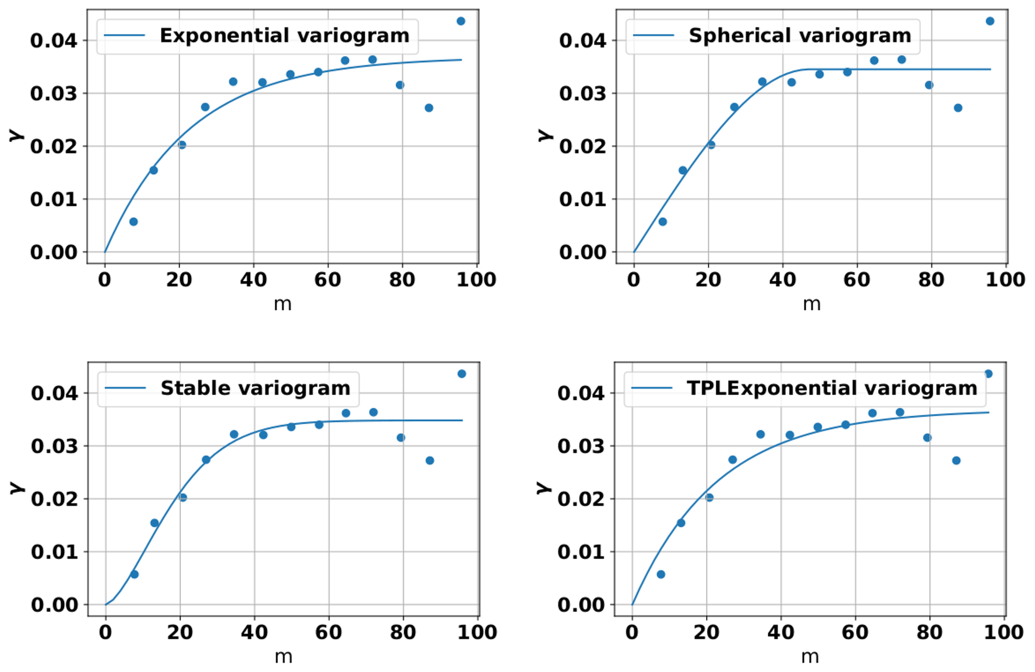
Figure 2 Scatter plot of the empirical variogram function for saturated log hydraulic conductivity presented by Wijaya et al. (2010), jointly with optimal fits using the exponential, the spherical, the stable and the TPL model function.

A crucial property of variogram models is the roughness information that is closely related to the mathematical concept of differentiability. The roughness α of a correlation function ρ(r) can be defined as (Wu and Lim, 2016)

$$\begin{array}{}\text{(9)}& \mathit{\rho }\left(r\right)\approx \mathrm{1}-k\cdot r^{\mathit{\alpha }}\mathrm{as}r\to \mathrm{0},\end{array}$$

with $\mathrm{0}<\mathit{\alpha }\le \mathrm{2}$ and k>0. Low values of α indicate a Gaussian process (not to be confused with the Gaussian variogram model) whose fields are very rough, whereas higher values indicate a process whose fields are very smooth.

For example, the Gaussian variogram model has a roughness information of α=2; the exponential and spherical models have α=1. The shape parameter of the Matérn model is directly connected to its roughness information with $\mathit{\alpha }=\min (\mathit{\nu },\mathrm{2})$, and in the case of the stable model the shape parameter coincides with its roughness information.

2.3 Numerical tools

As already mentioned, the data came from a variety of sources, most of which were scatter plots of empirical variogram functions in scientific articles and reports. In a first step, we digitized them with the freely available WebPlotDigitizer version 4.6. These data were joined into two different .csv files, one for aquifer sites and one for soils. These two data files of the extracted data are available online in the associated GitHub repository, which can be found at https://github.com/GeoStat-Examples/GeoStat-DB (last access: 11 January 2023) and is part of the collections of geostatistical examples of the GeoStat-Framework Python packages. The repository contains the whole workflow that generated all the results presented in the paper and ensures transparency and reproducibility of the workflow. This is particularly important since we consider the availability of the data set to be a key asset of our study. Making all data, results and the workflow that connects them available is therefore mandatory.

The data are stored in a series of subfolders that represent the different stages of processing. The data_raw/ folders contains raw data files, i.e., data on point-referenced measurements of hydraulic conductivity, transmissivity and permeability. Since some of the authors we contacted raised concerns about data ownership, we could not make all raw data available. In those cases, only the empirical variogram data are made available. The data_prep/ folders contain data on empirical variogram clouds. These are either derived from the aforementioned raw data or, more commonly, by digitizing scatter plots from journal articles and reports. The data_proc/ folder contains processed data, where all empirical variogram data are stored jointly in two files, one for data from aquifer sites and one for data from soils. They form the basis for all the analyses presented below. The data_stats/ folder contains the results of the geostatistical analysis, i.e., a number of .csv files that contain the best-fit, geostatistical estimates. Here, the .csv files follow the naming convention such that the file aquifer_statistics_gaussian.csv contains statistics from aquifer sites derived using the Gaussian variogram model, the file soil_statistics_matern.csv contains statistics from soils derived using the Matérn variogram model and so on. In addition, this folder contains statistics derived from the literature. The scr/ folder contains the Python scripts to perform these geostatistical analyses. These files are different depending on whether they are used to analyze aquifers or soils and what variogram model is used for the analysis. For example, the Python script empirical_aquifer_analysis_exponential.py analyzes data from aquifer sites using the exponential variogram model, the Python script empirical_soil_analysis_matern.py analyzes data from soils using the Matérn variogram model, and so on. The folder also contains the geostat_db_tools/ subfolder, where Python subroutines that are shared by all the other scripts are placed. Finally, the paper/ folder contains all data used in the production of this paper. This comprises the paper.tex file for the main text, the paper.bib file for the references used, the figures and all the scripts used to generate the figures from the results in the data_stats/ folder. This repository, therefore, contains all the data and the entire workflow for creating, reviewing and improving the results presented here.

3 Results and discussion

In the following, we will present and discuss the results of the analysis of the above data set using the tools presented in the previous section. For this purpose, we will focus on the statistical properties of the estimated variogram parameters. In particular, these are the length scale, the vertical and horizontal anisotropy, the nugget and the potential shape parameters of the variogram model function. In addition, we will investigate and compare how different model functions can describe empirical variogram data.

3.1 Comparison between different variogram model functions

Let us start with a comparison between the different variogram model functions using a goodness-of-fit criterion. The investigated model functions were the Gaussian model, the exponential model, the spherical model, the Matérn model and the stable model function. As the goodness-of-fit criterion, we chose the (pseudo-)R² measure, also known as the coefficient of determination, as implemented in the GSTools Python package. In this context, the (pseudo-)R² score indicates how much better a fitted model matches the data compared to a pure nugget model set to the mean value of the empirical variogram cloud.

Since not all model functions could provide a fit for all sites in the collected data set, we only used those sites for the comparison where the fitting procedure converged for all considered model functions. Overall, results between the different model functions were very similar when a clear plateau was reached within the covered spatial range (see left panel in Fig. 3 with the same data as presented in Fig. 2) but varied often substantially when no clear plateau was reached (see right panel in Fig. 3 with data from a low-permeability clay formation in Belgium; Huysmans and Dassargues, 2006). The similar accuracy of the different model functions was, of course, only true in the aggregate, i.e., when looking at the whole data set. It can, however, be explained with the overall similar behavior of variogram functions. Most differences between them are present at the origin of the functions, whereas for large spatial distances the different functions converge. The problems associated with empirical variogram data, which show no clear plateau with the covered spatial range, will be discussed in the following sections, where we will look into the behavior of different parameters of the model functions in more detail.

Table 2 Average R² scores for the different variogram model functions. For this comparison, only aquifer sites were used where all model functions resulted in a fit.

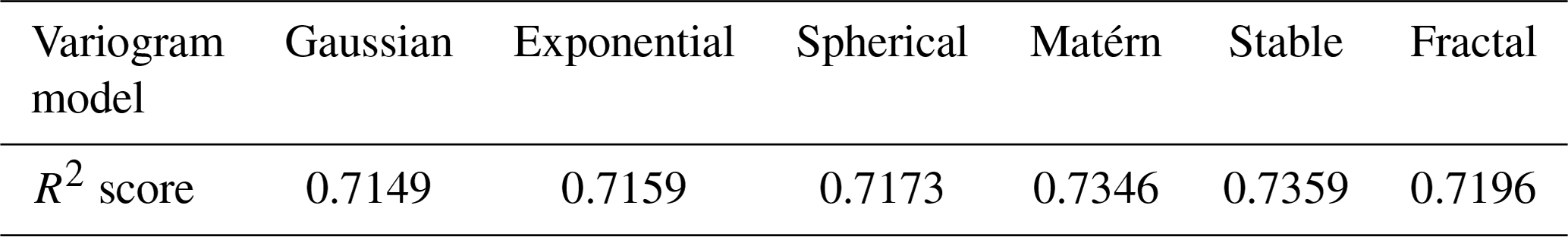
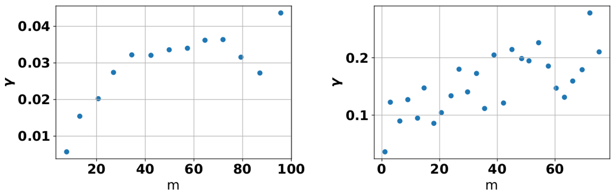
Figure 3 Scatter plot of empirical variogram function for saturated log hydraulic conductivity presented by Wijaya et al. (2010) (same data as presented in Fig. 2) and by Huysmans and Dassargues (2006).

In general, our results showed comparable goodness-of-fit measures for all investigated variogram model functions (see Table 2). Both the Matérn and the stable model function showed somewhat better R² scores compared to the others. This can be explained by the additional degree of freedom and therefore additional flexibility to match any given point cloud. However, whether these overall modest gains in accuracy are justified depends on the type of application and the needs of the practitioner. One formal way to quantify this trade-off are model selection criteria like the Akaike, Bayes or Hannan–Quinn information criteria, which combine goodness-of-fit measures with a penalty term for the number of parameters any given model has.

In this study, we did not perform such a quantitative model selection analysis since the overall goodness of fit was extremely similar for all investigated model functions. This was further substantiated when looking at a scatter plot of the individual R² scores comparing all functions pointwise. These comparisons showed that the similarities in accuracy between the different model functions were not only valid on the aggregated but also on the individual level (see Fig. 4 for a comparison of the exponential and spherical model functions). Our results therefore indicate that the selection of the most appropriate model does not have to be based on concerns about accuracy but can be guided by other considerations.

However, as will be shown and discussed below, the overall similar accuracy of the Gaussian, the exponential and the spherical model may be a result of the nugget value compensating for some of their lack in flexibility, which is restricted to the area of the curve near the origin. Given that the nugget value is not a pure convenience parameter but has a plausible physical interpretation, this behavior of the fitting procedure may be a liability depending on the modeling task.

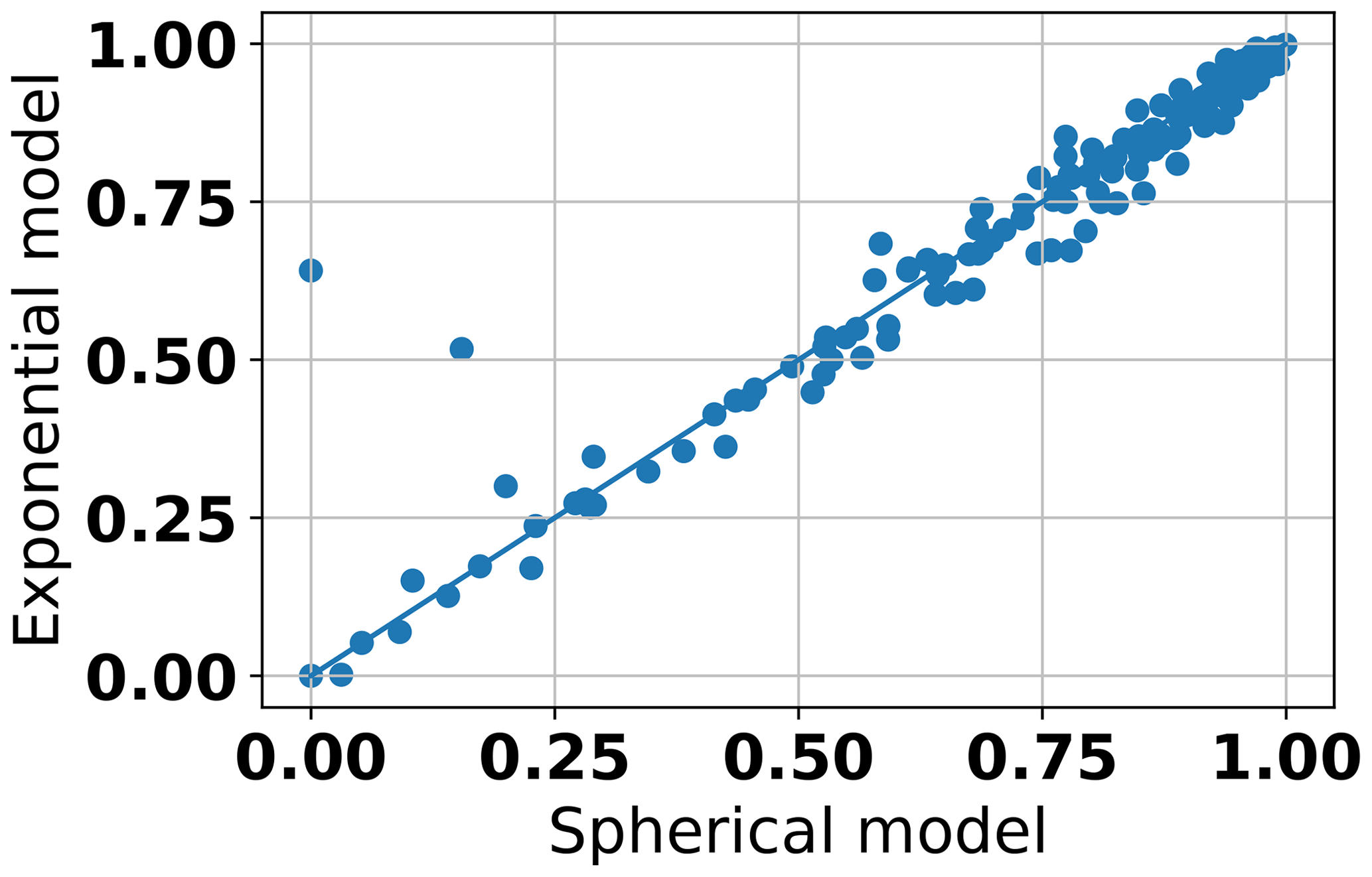
Figure 4 Scatter plot of the estimated R² scores of the exponential and the spherical model function.

It is known from the literature that the impact of the specific variogram model function on flow and transport simulations is mixed (Riva and Willmann, 2009; Jafarpour and Tarrahi, 2011; Heße et al., 2015). Given the overall similar accuracy, these results can interpreted such that the choice of what model function to use for any given task in subsurface hydrology can be driven by considerations of practicality and the specific aims of the task at hand.

One notable difference between the model functions was the number of sites for which our fitting procedure converged and consequently provided usable results (data not shown). The trend was such that the stable model showed the best performance, whereas the Matérn model showed the worst, with the other models being in between (data not shown). However, this study does not aim to present a thorough analysis of the numerical properties of the different model functions since these often depend on the specific implementation of the model functions themselves, the functions used provided by other packages and the specific setup of the fitting procedure. Using other software or tweaking the fitting procedure can therefore lead to a different behavior. We would consequently regard these observed differences as tentative and context specific. Regardless, in the following we will use results derived with the stable model as the default model, when investigating the behavior of specific parameters, if not specified otherwise.

3.2 Scale dependency

As we already discussed in the Introduction, the scale dependency of hydraulic properties like the correlation length is a well-known phenomenon from the literature (Neuman and Di Federico, 2003; Neuman, 2008; Colecchio et al., 2020). Therefore, we investigated this property empirically by using our data set and estimating the correlation lengths for all sites in the data set. The resulting set formed the basis for the following analysis. As mentioned earlier, we will only present results derived using the stable model. This was largely unproblematic, as the overall trend for most estimated parameters was the same regardless of the model function used. Only in cases where notable changes were observed or where we compared differences between the two models do we address them separately.

Our results confirmed a monotonous increase in correlation lengths with the maximum length scale for the case of both soil and aquifer sites (see Fig. 5). Using a log–log plot, we can clearly see an excellent linear relationship between both in the data set. As stated in the Methods section, the maximum length scale was defined here as the largest distance in the data set. In this study, this was identified with the largest distance between two observation points in the data set, typically two piezometer stations or observation wells. We also performed the same analysis with respect to the minimum length scale, which was identified with the smallest distance between two observation points in the data set. As expected, these results showed the same trend (data not shown).

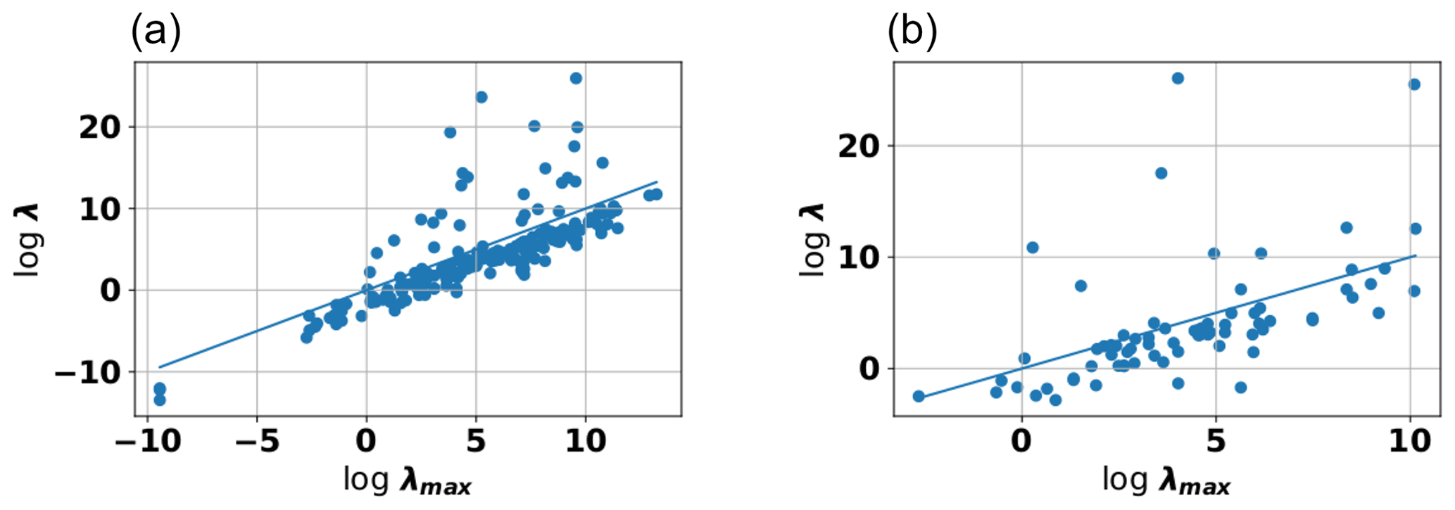
Figure 5 Log length scale vs. log maximum length for variogram models fitted to data from aquifers (a) and soil (b). The used variogram model function was the stable model.

It is not the purpose of this paper to enter into the long-standing debate about the nature of scaling effects and whether hydraulic variables represent intrinsic physical properties or whether they are introduced by the measurement process. However, it can be said that these data, and in particular the striking smoothness of the scaling behavior, provide strong evidence for the idea that the length scale of variogram functions is not primarily an intrinsic physical property of the medium but rather is influenced by truncation effects induced by the measurement process.

To further investigate the behavior of the estimated length scale, we also looked at the different estimates derived using different variogram models, namely the exponential, the spherical, the Gaussian, the Matérn and the stable model function. Results showed an overall strong linear correlation between the estimates for all investigated variogram models (see Fig. 6). While the slope of the regression plot varied, the overall trend was the same regardless of the used model. This demonstrates that all models capture the same underlying property of the empirical variogram cloud. Besides this strong linear correlation, a noticeable number of sites were outliers from this trend. To better understand these outliers, we took a closer look at a number of these sites. In all cases that we looked at, we found an empirical variogram function which had not yet reached a clear plateau. This phenomenon, that not all studied empirical variogram functions flatten with the studied spatial domain, has already been discussed above (see Fig. 3 and associated paragraph). When the long-range behavior of the full model function was not present in the data set, it resulted in a low sensitivity during the fitting procedure. The different variogram models, therefore, reacted differently when exposed to these data and provided sometimes strongly diverging estimates for those parameters most sensitive to the long-term behavior of the variogram function, namely the length scale and the variance. It should be noted that in the literature, we found a tendency to perform the fitting such that the plateau of the model function was reached within the given spatial range, probably by enforcing additional constraints, like fixing the variance, during the estimation procedure. Within this study, we did not enforce such conditions resulting in the observed divergence between the different models.

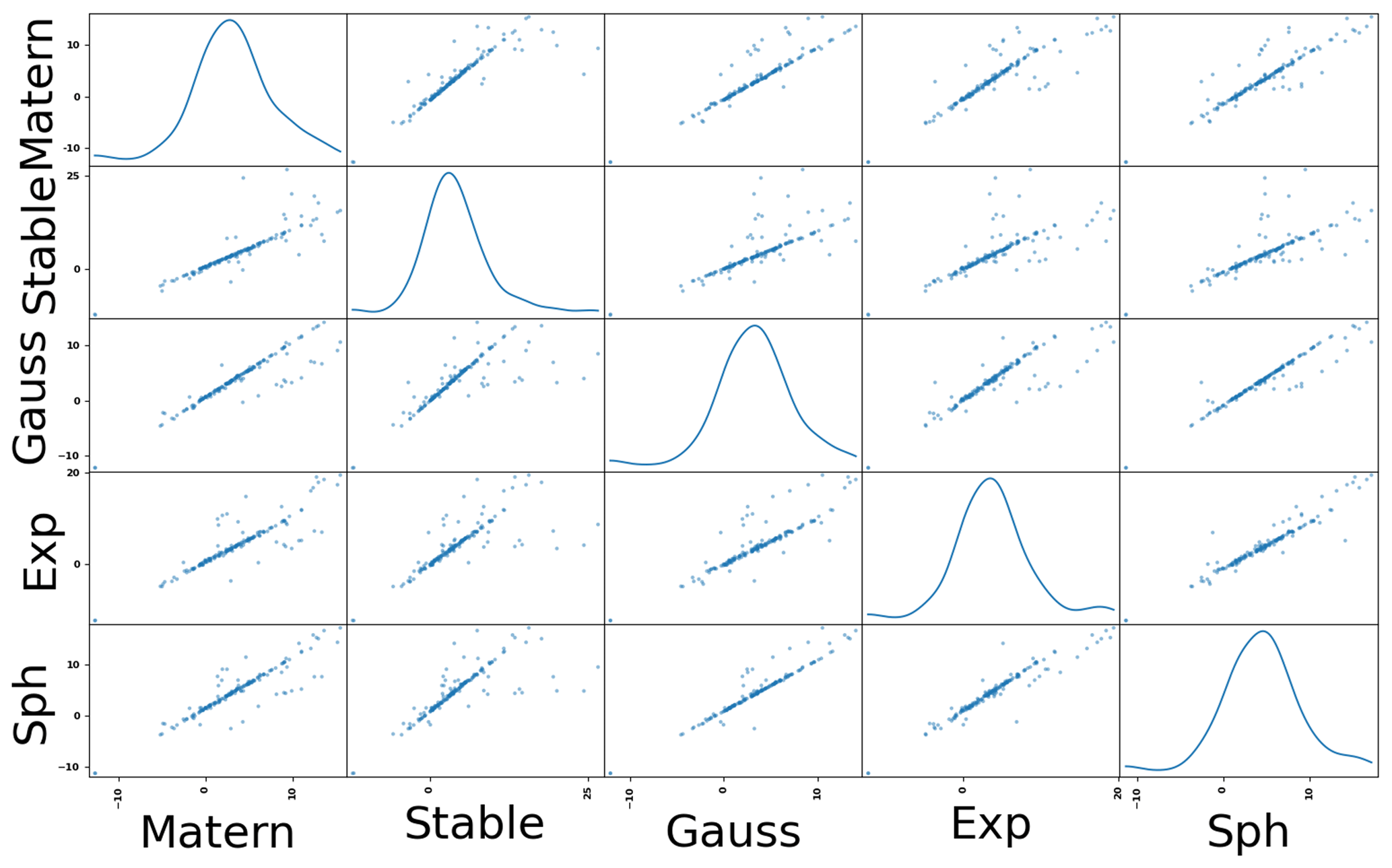
Figure 6 Scatter matrix plot for the estimated log length scales using the Gaussian, the exponential, the spherical, the Matérn and the stable model function.

To analyze the behavior of the scale dependency in more detail, we performed a kernel-density estimation for the residuals around the linear regression line presented in Fig. 5. The results showed a similar behavior for both aquifers and soils (see Fig. 7). In both situations, we saw that most estimated length scales were concentrated at around $\mathrm{1}/\mathrm{10}$th of the maximum length scale with a noticeable uncertainty around that estimate. This value coincides well with an empirical rule of thumb provided, e.g., by Neuman et al. (2007). Apart from this, both aquifers and soils showed estimated length scales that were larger than the maximum length scale present in the data set, a finding that is not explainable by a simple truncating process. These length-scale estimates which exceed the maximum length scale are not only substantially less common, their estimated value is also much less certain. This is due to the fact mentioned already that only a portion of the overall empirical behavior could be used for the fitting process, making the fitting procedure less stable.

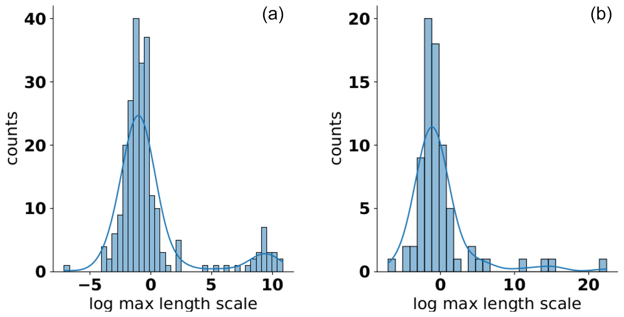
Figure 7 Histogram and kernel-density estimate of the residuals around the regression line of the data presented in Fig. 5 for aquifers (a) and soil (b).

All the above results present the length scale determined by fitting a stable variogram function to the empirical variogram cloud. However as discussed above, the correlation between the estimated length scale was high for all investigated variogram models. Using another model function consequently resulted in a very similar behavior (data not shown).

From a Bayesian perspective, the distributions of the residuals shown in Fig. 7 represent the uncertainty of a length scale estimate given a maximum length scale as a predictor. They are therefore a natural choice for the prior distribution of a Bayesian approach to variogram parameter estimation. Let us demonstrate this approach using the following steps. First, we perform a regression analysis for all sites in the data set for the variogram model one wants to use. Let us use aquifer sites only and the exponential model function since this is a widely used model. The regression model for the log correlation length given the maximum log length scale then results in

$$\begin{array}{}\text{(10)}& \log \mathit{\lambda }=\mathrm{0.985122}\log {\mathit{\lambda }}_{\max }-\mathrm{0.75734}.\end{array}$$

Here λ_max would be the said maximum length scale, i.e., the predictor of λ. This represents the knowledge one has regarding the expected correlation length. In the next step, we estimate the distribution of the residuals. This represents the uncertainty one has regarding the expected correlation length. In our case, we used a parametric model, namely a mixed model consisting of two independent Gaussian distributions:

$$\begin{array}{}\text{(11)}& \begin{array}{rl}p\left(\log {\mathit{\lambda }}_{\max }\right)& ={\displaystyle \frac{\mathit{\theta }}{{\mathit{\sigma }}_{\mathrm{1}}^{\mathrm{2}}\sqrt{\mathrm{2}\mathit{\pi }}}}{e}^{-{\left(\frac{\log {\mathit{\lambda }}_{\max }-{\mathit{\mu }}_{\mathrm{1}}}{\sqrt{\mathrm{2}}{\mathit{\sigma }}_{\mathrm{1}}}\right)}^{\mathrm{2}}}\\ & +{\displaystyle \frac{\mathrm{1}-\mathit{\theta }}{{\mathit{\sigma }}_{\mathrm{2}}^{\mathrm{2}}\sqrt{\mathrm{2}\mathit{\pi }}}}{e}^{-{\left(\frac{\log {\mathit{\lambda }}_{\max }-{\mathit{\mu }}_{\mathrm{2}}}{\sqrt{\mathrm{2}}{\mathit{\sigma }}_{\mathrm{2}}}\right)}^{\mathrm{2}}}.\end{array}\end{array}$$

Fitting this parametric model yielded the following estimates: ${\mathit{\mu }}_{\mathrm{1}}=-\mathrm{1.024}$, ${\mathit{\sigma }}_{\mathrm{1}}^{\mathrm{2}}=\mathrm{1.035}$, μ₂=9.488, ${\mathit{\sigma }}_{\mathrm{2}}^{\mathrm{2}}=\mathrm{1.318}$ and θ=0.8709. The goodness of the fit using these parameters can be seen in Fig. 8, indicating a very good representation of the estimated density. While a more complex model of, say, three Gaussian distributions may fit the kernel-density estimate even better, we consider the simpler model to be an acceptable parametric model for our case. This model, i.e., the regression and the prior distribution, can be used by a practitioner for the Bayesian geostatistical modeling of an unknown site.

Figure 8 Kernel-density estimate (solid) and fitted parametric model (dotted) of the residuals around the regression line for aquifers using the exponential model.

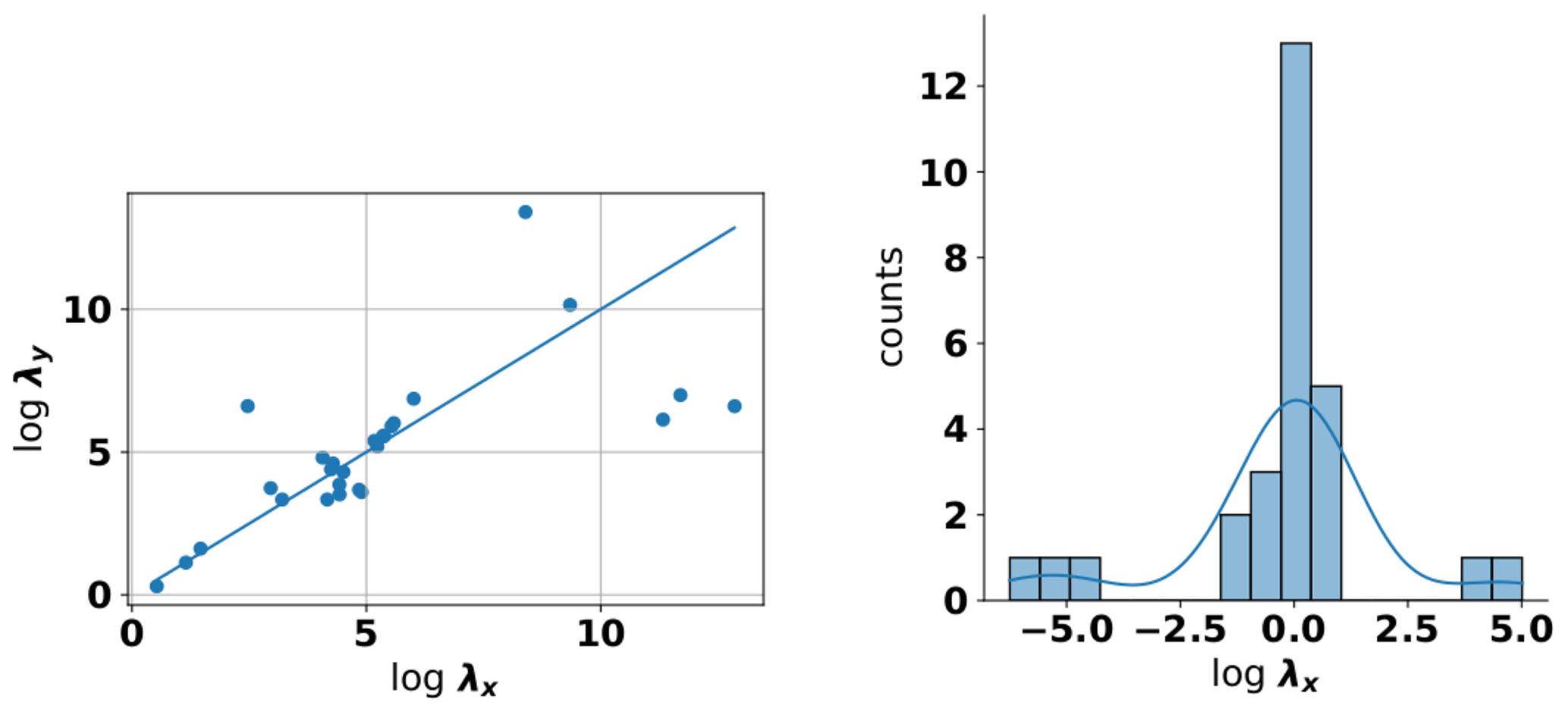
Figure 9 Scatter plot of both main horizontal length scales determined for aquifers using a stable model function (a) and (b) a kernel-density estimate of the residuals around the diagonal.

The above example is, of course, highly contingent on a number of factors. As already mentioned, using a different variogram model may lead to somewhat different estimates and maybe another parametric model may represent the inferred distribution more satisfactorily. In fact, we did follow the above procedure using other variogram models, which did lead to slightly different values for the regression line and the fit around the residuals. In addition, the data set used may change over time, or another type of clustering of the data may lead to different data sets and thus to different prior distributions. Regardless, the above example is a proof of concept on how to make use of the assets provided in this study. Of course all the scripts used to derive above results are available jointly with this paper. Practitioners are therefore free to repeat the analysis, review its results, and adapt it to their needs and applications.

3.3 Anisotropy

Having described the scale dependency of the correlation length, let us now look at the anisotropy of these estimates. As is well known, subsurface anisotropy is strongly pronounced between the vertical and horizontal direction but is often assumed to be negligible between the two horizontal direction.

Let us start with anisotropy in the horizontal direction. Our results showed a strong linear relationship between the estimated log length scales in both directions (labeled λ_x and λ_y in Fig. 9 left). The scatter is centered around the diagonal line, which is to be expected since the x and y directions are arbitrarily chosen and do not reflect any geological properties that could induce a meaningful difference between the two. Using the same procedure as above, we can also estimate the distribution around that center diagonal (see Fig. 9 right). In general, this estimate is based on significantly fewer data points (n=26 in case of the stable model) and is therefore less reliable compared to the density estimates presented above. As a result, a parametric model should be used to estimate the prior uncertainty, by following the above procedure. Given the tailing indicated in Fig. 9, the short-tailed Gaussian distribution, used in above example, may not be an appropriate parametric model for this situation. Instead, the use of a long-tailed distribution like the t distribution would be advisable.

Let us now look at the anisotropy between the vertical and horizontal directions. This anisotropy is known to be strongly pronounced due to the geological processes like sedimentation (Pyrcz and Deutsch, 2014). Our results confirm this anisotropy with some notable exceptions (see Fig. 10a). Overall, the number of sites used for this estimation was larger compared to the above case of horizontal anisotropy (n=48 for the case of the stable model). This number represents only sites in aquifers but could be increased if sites from soil variograms would be included. Since their numbers are small overall (n=4), we performed no dedicated analysis for this group alone.

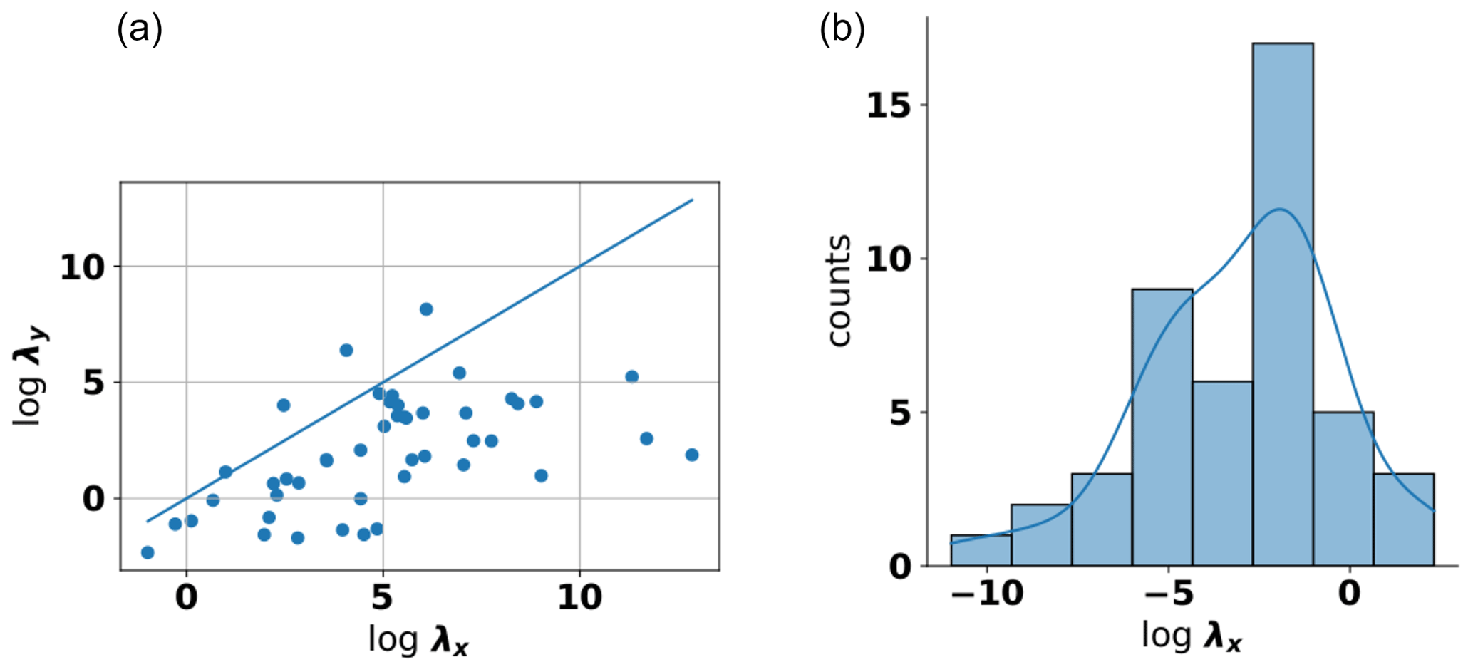
Figure 10 Scatter plot of horizontal and vertical log length scales determined for aquifers using a stable model function (a) and a kernel-density estimate of the residuals around the diagonal (b).

One of the most surprising results was the number of cases where the estimated vertical length scale is larger than the estimated horizontal length scale (see Fig. 10b). They are almost all caused by sites where the estimated length scale was larger than the maximum length scale. This indicates that it may be, at least in part, caused by the resulting uncertainty in the estimation procedure. It is, therefore, not clear whether these results should be used to derive a prior distribution. If they were included, the resulting distribution would again show a long-tailed behavior. Like in the case of the horizontal anisotropy, a parametric fitting procedure using the t distribution could be a good candidate (see Fig. 10b).

3.4 Nugget value

The next variogram parameter we investigated was the nugget parameter. This parameter describes the variance at the lag value of zero, i.e., how much measurements differ that are taken at effectively the same location. Such differences are often interpreted to represent two very different phenomena; first they may refer to measurement errors or second to unresolved variations in the measured variable below the measurement scale (Rubin, 2003; Kitanidis, 2008).

To investigate the behavior of the nugget parameter, we estimated its value using the stable model function and fitted it against our collected data set. For the analysis, we normalized the value of the nugget against the variance, making sure its value was between 0 and 1.

Results showed a somewhat similar behavior for the estimated distribution of nugget values for both aquifers and soils. In general, most nugget values were close to 0 in both cases, indicating a small or negligible measurement error or subscale variabilities. Regardless, a substantial portion of the estimated nugget values were found above the value of 0.5, meaning that large uncertainties are present in many data sets. Such higher values for the nugget were more common for data sets from soils, leading to an effectively bimodal behavior of the resulting density estimates. It should be noted that our soil data set was smaller compared to the aquifer data set (n=71 and n=215 for soil and aquifer sites, respectively). As regards a suitable parametric model for this observed behavior, it is clear that a Gaussian or t distribution is not a viable candidate, due to the potential range of values being bounded between 0 and 1. Any parametric model function that is to be fitted against the sample should, therefore, be chosen to honor both these boundaries as well as the general behavior indicated in the kernel-density estimate. Given the observed behavior in Fig. 11, a mixed model using the beta distribution or a truncated lognormal distribution may be viable candidates.

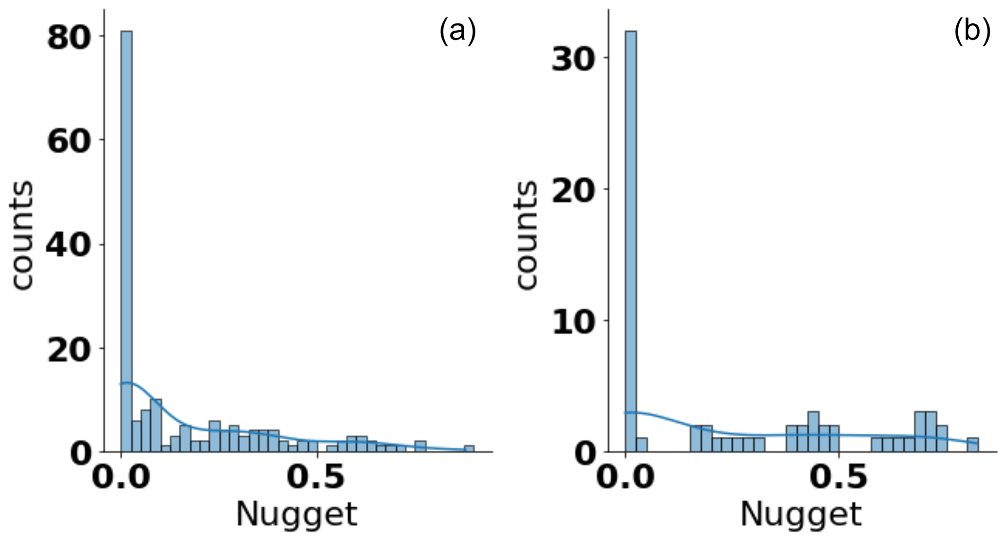
Figure 11 Kernel-density estimate of the estimated nugget values for aquifer (a) and soil (b) sites. The variogram model used was the stable model.

To investigate how the nugget value differed between the variogram model functions, we also compared their respective estimates. Our results showed a strong linear correlation between the estimated nugget of the stable model and the Matérn model (see Fig. 12a), which shows the similarity between both model functions. On the other hand, plotting the estimated nugget of the Gaussian model vs. the exponential model shows substantially larger differences between the two (see Fig. 12b). This is due to the different behavior of these two models for small lag values. Whereas the exponential model exhibits a steep gradient, the Gaussian model is essentially flat in this region. The different nugget values are therefore an artifact of the fitting procedure, which tries to compensate for this difference through adjusting the nugget value. This demonstrates that prior distributions for this value should be considered as model specific and should not simply be transferred between different model functions.

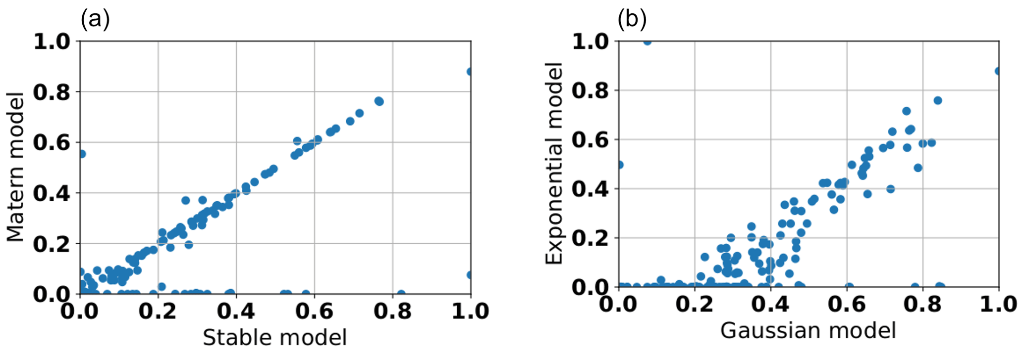
Figure 12 Scatter plot of the estimated nugget values for the stable model vs. the Matérn model (a) and Gaussian model vs. the exponential model (b). All data were drawn from aquifer sites.

The estimated nugget values of the spherical model showed the highest correlation with the nugget values of the exponential model but a lower correlation with the nugget values of all other variogram model functions examined (data not shown). This is due to the similar behavior of the spherical model and the exponential model at small lags, again showing the relationship between this near-origin behavior of the model function and the ability of the nugget model to compensate for possible inconsistencies between the empirical variogram and the behavior of the model function. Although all results shown were derived from aquifer sites only, the use of data from soils also supports these statements.

3.5 Shape parameter

Many common variogram model functions like the exponential and the Gaussian model are fully defined by specifying the length scale, the variance and the nugget value. There is, however, a class of variogram model functions that feature an additional degree of freedom. In the following, we will call this additional parameter the shape parameter.

In the case of the well-known Matérn function, this parameter is known as the roughness parameter ν. This name refers to the fact that its value is directly related to the roughness of the resulting spatial random field (Banerjee and Gelfand, 2003; Diggle and Ribeiro, 2007). The relationship is such that a low value means a high roughness, with the value of ν=1.0 resulting in a random field that has no derivatives whatsoever, i.e., infinite roughness. A Matérn model function with such a low value is mathematically identical to the exponential model function. On the other end of this spectrum, a very high value of ν→∞ results in a field with an infinite number of derivatives, i.e., infinite smoothness. A Matérn model function with such a high value of ν is mathematically identical to the Gaussian model function.

Our results show a somewhat bimodal behavior of the resulting frequency distribution of estimated ν values (see Fig. 13). This behavior is very similar for both aquifers and soils. The first cluster of the estimated shape parameter ν is found for very small values, with most values being at or near ν=0.5. This indicates that an exponential model function would perform with similar accuracy in these cases. On the other hand, a second cluster can be found for ν>20. Although the Matérn function only converges to the Gaussian function in the limit of ν→∞, it should be noted that already for values of ν>10, both functions become virtually indistinguishable. The roughness parameter has little impact beyond such a high value, meaning that it barely changes the behavior of the function anymore. This means that a Gaussian model function would be able to similarly describe cases in this second cluster very well.

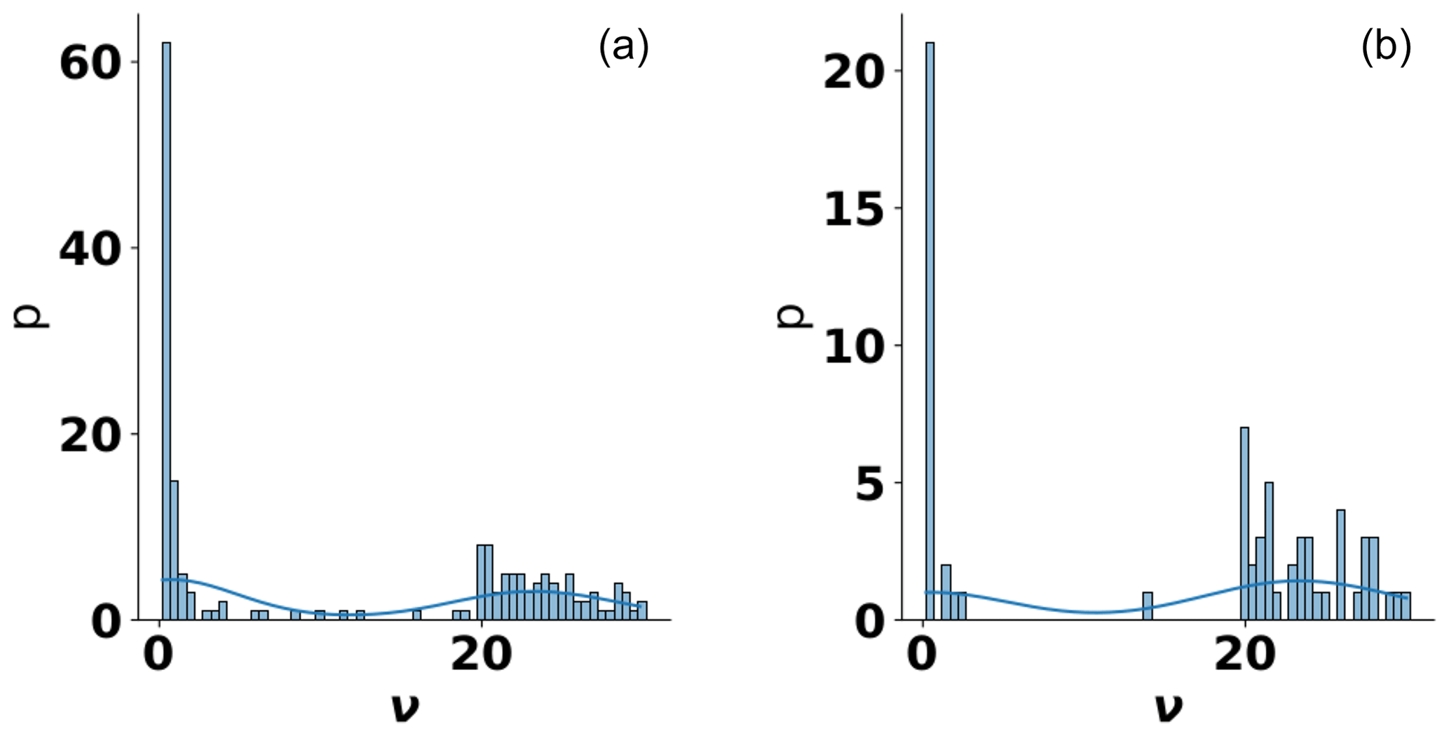
Figure 13 Kernel-density estimate of the estimated roughness parameter ν of the Matérn variogram model function for aquifer (a) and soil (b) sites.

These observations support a number of conclusions. First, despite the roughness parameter spanning a significant range, most of its values fall into two intervals, both of which can be approximated well with a more common model function, namely the exponential and Gaussian function. Second, the number of cases where a Gaussian model function would be a good fit is larger than expected. Due to its high smoothness, the Gaussian model function is sometimes considered unrealistic (Stein, 1999). This assessment is not supported by our findings, at least not from a simple fitting perspective. Finally, the Matérn model function is still a relevant model function since it may not be clear in advance which classic function, i.e., the Gaussian or the exponential, can provide a better performance.

In the next step, we analyzed our data set using the stable variogram model function. The shape parameter of this model function is denoted as α. Our results again show a roughly bimodal behavior of the resulting frequency distribution of α (see Fig. 14). It should be noted that the shape parameter α is defined between 0 and 2, and many values are found for α=2. Still, the overall similarity shows a connection between the two shape parameters of the Matérn and the stable mode functions.

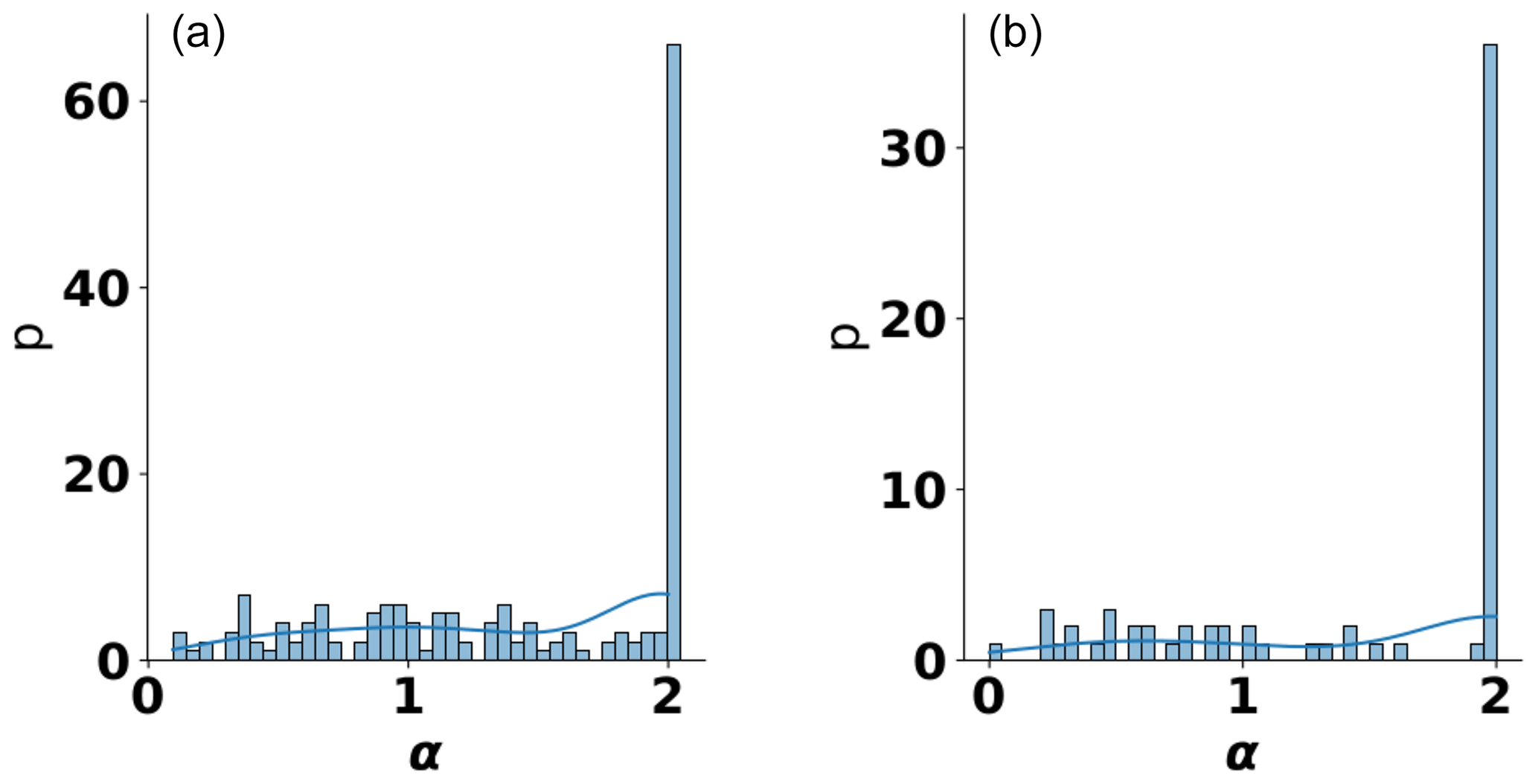
Figure 14 Kernel-density estimate of the estimated shape parameter α of the stable variogram model function for aquifer (a) and soil (b) sites.

To better understand this connection between the shape parameter ν of the Matérn model and the shape parameter α of the stable model function, we performed a regression analysis for those sites where both model functions did result in a fit. Our results showed a very similar behavior for both aquifers and soils (see Fig. 15). As can be seen, the scatter plot reveals that most points in the plot fall into two distinct correlation regimes between ν and α. First, for smaller values of ν, representing an exponential-like behavior of the Matérn function, we see a linear correlation between the two with a very flat slope. This flat slope is caused by the strong clustering of sites where ν≈0.5 For high values of ν, representing a Gaussian-like behavior of the Matérn function, we see a nearly vertical behavior; i.e., a larger range of ν values now corresponds to a very small range of α values. The latter is caused by the truncation behavior of the stable model, which is confined to values between 0 and 2. This means that the range of ν values, representing a Gaussian-like behavior, gets mapped into a very small interval of α values close to 2 (see behavior in Fig. 15).

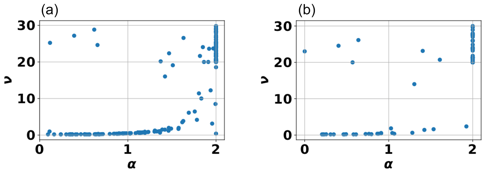
Figure 15 Scatter plot of the estimated shape parameter values for aquifers (a) and soils (b). Here, ν is the shape parameter of the Matérn model, and α is the shape parameter of the stable model.

We can draw two conclusions from these observations. First, the shape parameter α of the stable model is indeed related to the shape parameter ν of the Matérn model since both are directly connected to their respective roughness information as described above. Second, the confined parameter range of the stable model is not a drawback from a practical point of view since the sensitivity of the Matérn model becomes extremely low for larger values of ν. In fact, from a numerical perspective, this limitation of the parameter range is an asset since it improves the performance of an optimization algorithm necessary for the fitting procedure. Although this study does not aim to investigate this issue in detail, we did indeed observe a much higher numerical stability of the stable model compared to the Matérn model. This stability was observed both in terms of the number of steps necessary to find an acceptable fit between the model function and the empirical variogram function and in terms of the number of sites for which optimal parameters could be found. Although the name of this model is derived from the stable distribution (Wackernagel, 2003), it, therefore, also describes its numerical behavior, a connection which is no doubt a coincidence.

Finally, we also looked at the Hurst coefficient, which can be interpreted as the shape parameter of the TPL variogram model function. Results for the Hurst coefficient also show a roughly bimodal behavior, with many values being clustered near the boundaries of the values' range (see Fig. 16b). It shows the low sensitivity of the Hurst coefficient for the data sets used. This is not surprising given that the highest sensitivity is with respect to the near-origin behavior, where often fewer data points were available. In addition, the nugget parameter also has its highest sensitivity in this region. Both these facts result in a situation where the overall sensitivity of this parameter is rather low. In addition, we also looked at the overall trend of the Hurst coefficient with respect to the length scale and found no relationship between the two (see Fig. 16a). Given, however, the low sensitivity of the Hurst coefficient toward the available data that has already been established, this result has to be interpreted carefully.

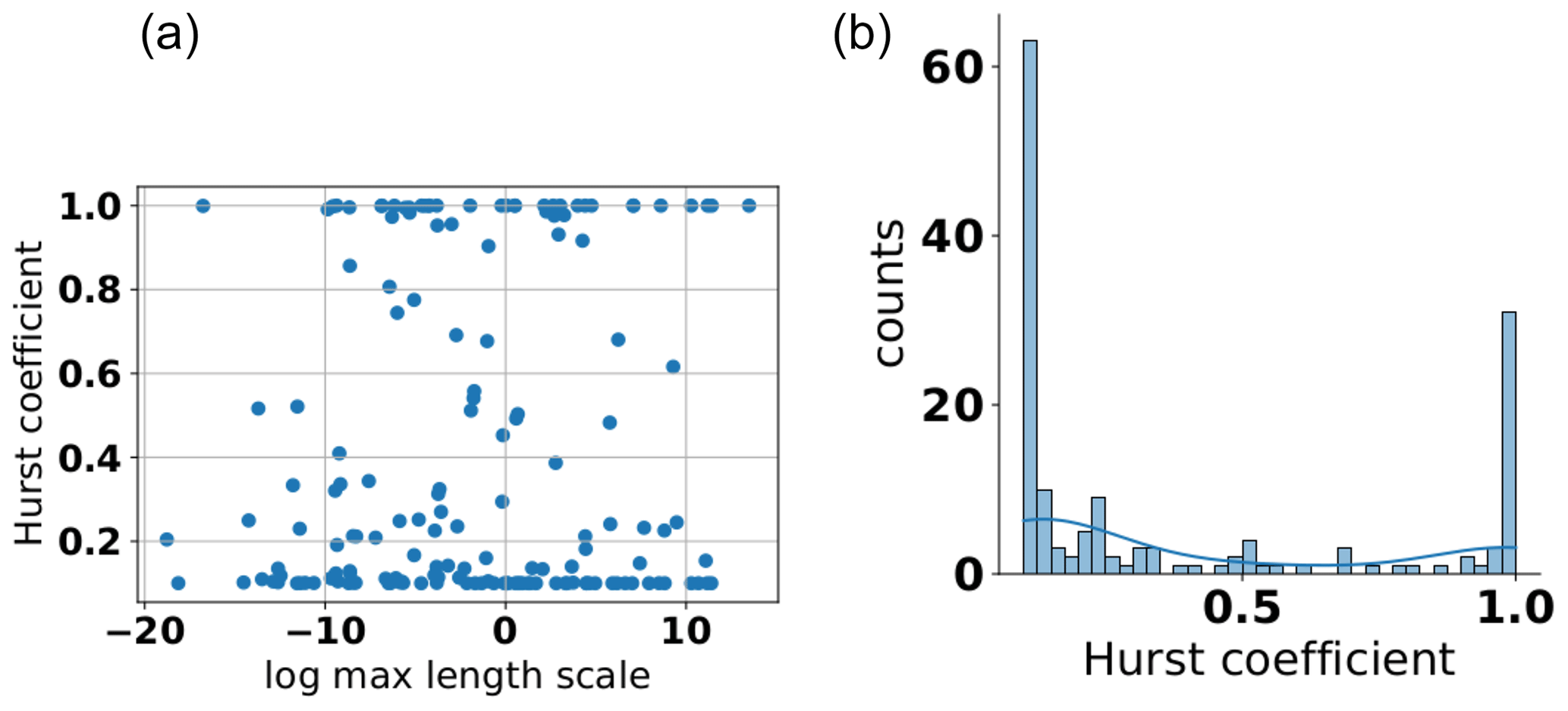
Figure 16 Scatter plot of the estimated Hurst coefficient for aquifer sites (a) and its kernel-density estimate (b).

3.6 Critical assessment of results

In addition to presenting and discussing our results, we would also like to assess our work critically, in the sense of determining both possible weak points as well as limits to their applicability. This will help practitioners to apply our results and use our data more appropriately and avoid misuse.

The first topic that we would like to address concerns the problem of publication bias or survivor bias (Schmitz et al., 2012). This is caused by the fact that our data set is based on published data alone, meaning that only data which both the author(s) and editor(s) deemed suitable for publication could end up in our collection. This notion is for instance substantiated by the fact that all empirical variogram functions we found produced viable variogram parameters when they were analyzed by the respective author(s) of the study. However, when we re-analyzed them, a certain number of sites resulted in a fit where the estimated length scale was larger than the largest length scale in the study. This indicates that authors choose not to publish results that they consider unsatisfactory for various reasons. As a result, our data set is not a random sample of aquifers and soils from all over the world but skewed toward sites where an acceptable variogram analysis was achieved, whereas problematic cases may have been left out. Having a non-random data set is a serious challenge for any statistical investigation. Whether this is a problem, however, depends on the type of application. For a typical geostatistical characterization of a site, it may not be of relevance. After all, practitioners of subsurface geostatistics by definition are only going to use these results for sites which they deem appropriate for a variogram analysis. For such an application, the data sets used for our investigations may, therefore, not be biased in any relevant way. Still, there are applications where the topic of survivor bias should be considered carefully. In any situation where our data set is to be used for inferring general properties of aquifers and soils, proper care in the interpretation of one's results is, therefore, advised.

Another challenge present in the data sets found in the literature was the general lack of data for short lags. Most of these data sets were generated from observation networks that followed a regular grid. This makes sense in practice, as most studies try to maximize the spatial coverage of their measurement campaign but can only use a limited number of observation points due to budget constraints. However, from a variogram estimation perspective, this is problematic. Parameters such as the nugget or shape parameter are most sensitive to behavior near the origin, i.e. at small distances compared to the characteristic length scale. If the data in this important region are sparse or noisy, the estimation procedure becomes more error prone. A good way to balance budget constraints with the need for better information at close distances would be to arrange at least some of the observation points in a logarithmic fashion (Müller et al., 2021).

Another possible challenge concerns the variable number of data points used for the inference of the different density distributions of variogram model parameters. While any density estimation improves with the number of samples being used, there are no widely agreed rules as to how many sample points are necessary for an acceptable estimation procedure (Dell et al., 2002). In addition, different features of a distribution need different numbers of sample points, with higher moments or higher dimensions needing more data (Silverman, 1986). This is particularly problematic for densities having uncommon features like long tails, being highly skewed or being multi-modal. In general, non-parametric estimators can handle the challenge of uncommon distributions well but require a large sample size. On the other hand, parametric approaches require much fewer data but can lead to model errors if the parametric model is far from the true density (Li and Racine, 2006). In order to account for this problem, we presented an approach where we started with a non-parametric method, like kernel-density estimation and subsequently interpreted the results within the context of a suitable parametric model for the inferred behavior of the underlying distribution. We then used the said parametric model for estimating the density. Of course, this is only one possible approach to addressing this challenge, and practitioners may find other approaches more appropriate depending on their circumstances. Since all data and analyses are openly available, they can easily adapt this approach to their needs.

Related to this topic is the problem that any inference based on past observation may miss features that are not represented in the used data set (Billot et al., 2005; Gilboa et al., 2010). For the results presented here, this is not of primary concern since all investigations were performed with respect to properties which are known to be relevant based on prior experience, i.e., the parameters of widely used variogram models. Still, the data set collected for this study can be used to investigate a number of questions, some of which have been alluded to above. In these cases, this challenge should be kept in mind.

Another topic that needs to be addressed is the fact that some of the variogram data we used for the analysis were provided in clustered form such that they were labeled as coming from the same site but representing different categories. In the data set, we marked these variograms by using the same site_id but distinguished them by the label geological_unit. As mentioned in the Methods section above, the reason that the same site label was used for different data sets differed in each situation. In some cases, the authors separated the data according to different geological layers; in some cases the separation represented geological subunits, subdivided by the authors according to their domain knowledge; in some cases it represented several actually different sites that were combined into a single measurement campaign; and in some cases it was not clear according to which criterion the separation was made. The label geological_unit does therefore represent a number of different and disparate situations. Still, the sheer fact that they may be similar can pose a problem from a statistical point of view since variograms from the same site, regardless of what that term meant in that particular study, may be correlated to a certain extent. This problem is known as pseudoreplication in the literature (Hurlbert, 1984). Using only a single data set per site would avoid this problem but reduce the overall amount of data available. On the other hand, using all the data risks giving too much weight to some sites, where several variograms are available. To determine the relevance of this risk, we looked at variograms derived from different subunits and saw moderate correlations in some cases and none in others. Within the scope of this study, we did therefore treat these different subunits as independent sites. To properly account for the possibility of within-site correlations, however, a hierarchical model could be employed (Cucchi et al., 2019). In such a hierarchical model such within-site correlation could be estimated from the data provided enough data points are available. Within the scope of this study, we did not perform such an investigation, but the availability of the data set, where variogram data from the same site are marked as such, makes it possible for future investigations to address this topic, if necessary.

The last topic we should discuss is the fact that the empirical variogram functions do not represent raw data but are already processed to a certain degree. This means that these data implicitly contain modeling assumptions that were used when these empirical variograms were determined and are no longer present. As a result, it makes them somewhat less comparable. From a Bayesian point of view this means that the density estimates contain modeling uncertainty, which may, depending on the need of the practitioner, result in a larger uncertainty. This issue is unproblematic from a cautionary point of view, since the result is simply an increase in uncertainty. On the other hand, it is unsatisfactory due to the said increase in uncertainty, which means a loss of information, compared to the use of the raw data instead. For instance, for the results presented in this paper, we did not use tertiary data of site statistics due to the modeling uncertainty associated with them but only made them available at the online repository. While primary data have the lowest modeling uncertainty, their overall numbers were too small. As a result, secondary data formed the majority of the data providing a compromise between sample size and accuracy.

Finally, we want to emphasize that a purely data-driven analysis is not a substitute for but rather an addition to good domain knowledge and site-specific expertise. First, our analysis does only provide the prior distribution for a number of variogram parameters. As such, this is only the first step for a full characterization, and site-specific data may lead a practitioner to very different conclusions depending on the circumstances. Furthermore, our analysis has also shown how elusive a number of parameters are if only fitting concerns are taken into account. This is particularly true for the near-origin behavior (e.g., nugget value) and parameters that depend on it (e.g., the shape parameter). As such, a critical and careful attitude towards data-driven methods is necessary to prevent overconfidence and misuse of this otherwise important tool of geostatistics.

4 Conclusions

In this study, we have presented two different advances for the field of subsurface geostatistics: first, a data set of empirical variogram functions from a variety of different locations around the world, and, second, a series of geostatistical analyses aimed at examining some of the statistical properties of such variogram functions and their relationship to a number of widely used variogram model functions.

The data set collected for this study is freely available in the online repository associated with this paper (see the “Code and data availability” section below). It can therefore be used by practitioners to replicate our analyses, extend them with additional data and adapt them to their needs. They can also use it to explore new questions not covered here. Finally, we explicitly encourage practitioners to both expand the data set and extend the range of metainformation associated with it. This would allow additional questions to be answered and the scope of the data presented here to be broadened.

As regards our analyses of the said data set, we have derived a set of frequency distributions for the parameters of variogram models that can be used as prior distributions for Bayesian geostatistical applications. Since these prior distributions already contain a considerable amount of information, their use will result in a higher information content in the posterior. Given the overall dearth of subsurface data and the often high exploration cost, such an additional source of information presents a valuable asset for a geostatistical characterization of a soil or aquifer site.

In addition, we investigated the viability of different variogram model functions for modeling the empirical variogram cloud. Our results showed an overall similar accuracy of all investigated variogram models even though some feature 1 additional degree of freedom. This overall similar accuracy supports the notion that variogram models can be primarily chosen by the practitioner based on other considerations like familiarity, applicability and availability.

Finally, our investigation revealed the distribution of some geostatistical features of subsurface sites. First, the widely observed scale effect of many subsurface properties is strongly pronounced for the characteristic length scale of the heterogeneities. This observation supports the conceptualization of the subsurface as a fractal medium, where heterogeneities appear on any scale of observation, and their apparently finite length is, at least in part, a finite-size effect caused by the truncation of the measurement process. Next, the nugget value, a feature representing measurement errors and subscale variability, is widely distribution over its possible range, an observation that is exacerbated by the fact that simpler variogram models may tend to compensate with the nugget parameter for a mismatched model behavior at short distances. Finally, that behavior at short distances is strongly connected to the roughness of said heterogeneities. Our results show that most sites fall into two distinct categories depending on that roughness, i.e., either having very high or very low roughness. If this behavior is to be represented correctly, a more flexible model function, e.g., the Matérn or stable model, is to be used.

To extend the results and data discussed here, a number of options can be considered. First, expanding the number of sites covered and adding more features could reduce the uncertainty in the prior distributions. Using the above workflow, the uncertainty in these distributions represents the uncertainty of the entire data set and thus assumes that a particular site is a random draw from that set. However, it is not mandatory to use such a large and therefore statistically highly variable population. In fact, there is no unique population from which any given site needs to be considered to be randomly drawn from, a notion that is known in statistics as the reference class problem (Hajek, 2007; Hajek and Hitchcock, 2016). As a result, it is advantageous to use the most precise reference class for which a large enough sample is still available, thus striking a balance between precision and accuracy (Wallmann, 2017). In subsurface geostatistics, this would mean only using sites for the transfer of information which are similar to the given site based on some criterion of site similarity (Kawa et al., 2022). Yet, being able to limit one's analysis to a smaller, more appropriate and less variable cluster of similar sites would require a large population of sites, arguably larger than the current data set.

Another possible venue for further study could be to establish a connection between certain variogram properties and varied geological settings (sediments, rocks, porous versus fractured media) as well as the measurement technique used. This would again necessitate the addition of geological features to the database itself, a task that was beyond the scope of the current study. If done, it could, e.g., help practitioners to discern how such features affect variogram behavior.