140-year daily ensemble streamflow reconstructions over 661 catchments in France

The recent development of FYRE (French hYdroclimate REanalysis) Climate, a high-resolution ensemble daily reanalysis of precipitation and temperature covering the 1871–2012 period and the whole of France, offers the opportunity to derive streamflow series over the country from 1871 onwards. The FYRE Climate dataset has been used as input for hydrological modelling over a large sample of 661 near-natural French catchments using the GR6J (Génie Rural à 6 Paramètres Journaliers) lumped conceptual model. This approach led to the creation of the 25-member hydrological reconstructions, HydRE (Hydrological REconstruction), spanning the 1871–2012 period. Two sources of uncertainties have been taken into account: (1) the climate uncertainty using forcings from all 25 ensemble members provided by FYRE Climate and (2) the streamflow measurement error by perturbing observations used during the calibration. Further, the hydrological model error based on the relative discrepancies between observed and simulated streamflow has been added to derive the HydREM (Hydrological REconstruction with Model error) streamflow reconstructions. These two reconstructions are compared to other hydrological reconstructions with different meteorological inputs, hydrological reconstructions from a machine learning algorithm, and independent and dependent observations. Overall, the results show the added value of the HydRE and HydREM reconstructions in terms of quality, uncertainty estimation, and representation of extremes, therefore allowing us to better understand the variability in past hydrology over France.

1 Introduction

Long time series of streamflow observations allow us to better apprehend the effect of current changes on hydrology and to challenge our water management with ancient extreme events such as low flows or floods (Slivinski, 2018). However, even in a data-rich country such as France, the network of observations available before the 1970s is quite sparse (Caillouet et al., 2017). The use of the sole observation-based information can lead to hazardous extrapolation of trends (Giuntoli et al., 2013) or a truncate vision of past extreme events. Furthermore, multidecadal variations have been observed in the few records available of streamflow (Bonnet et al., 2020, 2017; Boé and Habets, 2014) or in variables that are closely related, such as precipitation (Willems, 2013; Slonosky, 2002), showing the importance of long-term reconstructions.

Another way to obtain long time series of streamflow is to make use of a hydrological model (see for example Brigode et al., 2016; Crooks and Kay, 2015; Smith et al., 2019). However, this approach requires long-term climatic information based on observations, downscaled global climate models/reanalysis, regional climate models, or surface reanalyses. Over France, several studies have already used this approach to reconstruct long-term streamflow time series (Caillouet et al., 2017; Kuentz et al., 2015; Dayon et al., 2015; Bonnet et al., 2017, 2020). Those studies mainly use, as forcings for hydrological models, climate reconstructions based on downscaling large-scale reanalyses spanning the entire 20th century, such as the 20th Century Reanalysis (20CR; Compo et al., 2011) and the ECMWF Reanalysis of the 20th Century (Poli et al., 2016). Some of the climate reconstructions also integrate information from long-term observed time series to constrain the statistical downscaling methodology (Kuentz et al., 2015; Bonnet et al., 2017, 2020). However, most of these studies do not provide any uncertainty in the result and/or do not integrate all available in situ observations.

To make up for those shortcomings, the FYRE Climate reanalysis (French hYdroclimate REanalysis; Devers et al., 2020a, 2021), a high-resolution 25-member ensemble daily reanalysis of precipitation (Devers et al., 2020b) and temperature (Devers et al., 2020c) covering the period 1871–2012, has recently been produced. This new dataset originates from an offline data assimilation scheme (Bhend et al., 2012) based on the widely used ensemble Kalman filter (Evensen, 2003). The prior ensemble, called SCOPE Climate (Spatially COherent Probabilistic Extension Climate; Caillouet et al., 2016, 2017, 2019), originates from a statistical downscaling of the 20th Century Reanalysis (20CR; Compo et al., 2011). FYRE Climate assimilates historical daily observations of precipitation and temperature from the Météo-France database.

This study proposes to make use of the new FYRE Climate reanalysis as forcings into the lumped continuous rainfall–runoff GR6J (Génie Rural à 6 Paramètres Journaliers; Pushpalatha, 2013) to create long-term hydrological reconstructions over a large set of near-natural catchments in France. The modeling methodology builds on the work of Caillouet et al. (2017) but additionally takes into account several sources of uncertainties: (1) the climate uncertainty using forcings from all 25 ensemble members provided by FYRE Climate, (2) the streamflow measurement error by perturbing observations used during the calibration, and (3) the hydrological model error by post-processing based on the relative discrepancies between observed and simulated streamflow (Bourgin et al., 2014). The modeling methodology led to the creation of two 25-member reconstructions providing daily streamflow over a set of 661 near-natural French catchments over the 1871–2012 period:

• HydRE (Hydrological REconstruction), including sources of uncertainty (1) and (2), and

• HydREM (Hydrological REconstruction with Model error), additionally including uncertainty (3) related to the hydrological model error.

The paper is organized as follows: Sect. 2 introduces the observed streamflow series and two reconstruction datasets based on the same hydrological model (Safran Hydro and SCOPE Hydro; Caillouet et al., 2017), as well as alternative and larger-scale reconstructions from Ghiggi et al. (2019a). Section 3 describes the hydrological modelling strategy, the calibration methodology, the definition of the model error, and the creation of the HydRE and HydREM hydrological reconstructions. Their validation through different comparisons is presented in Sect. 4, and detailed example uses of the reconstruction – the study of an extreme flood event in 1890 and monthly records of high and low flows – are also shown. Finally, several points are discussed in Sect. 5, and conclusions are drawn in Sect. 6.

2 Hydrological data

2.1 Observed streamflow

For this study, daily observed streamflows for different sets of catchments are extracted from the national HydroPortail (https://www.hydro.eaufrance.fr/, last access: 12 July 2024) database (Leleu et al., 2014); see Fig. 1.

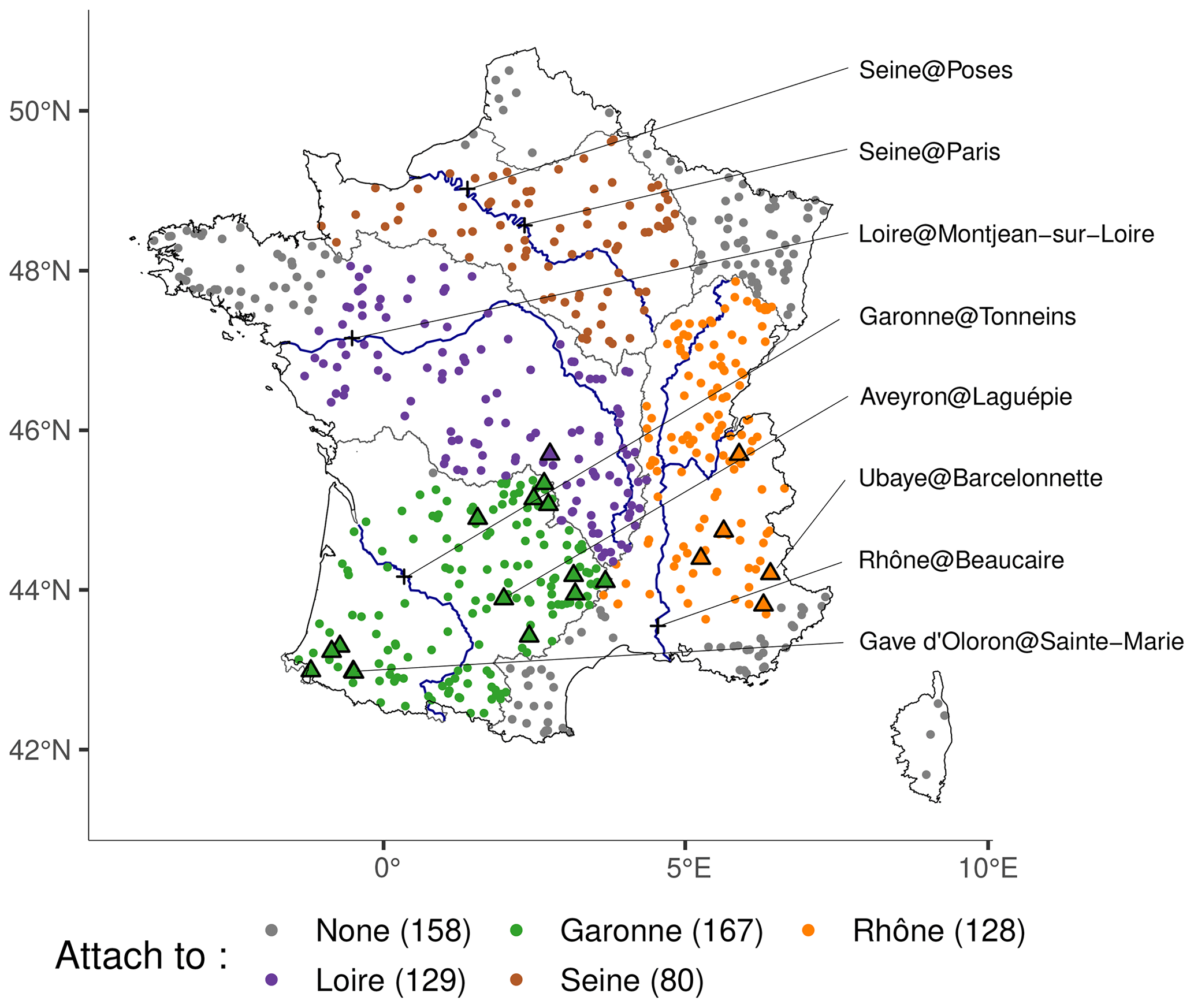
Figure 1 Location of the 661 outlets of the simulated catchments (circles and triangles) and of the four main rivers of France (crosses). Triangles indicate the outlets of the 20 catchments with the longest observational records. The three triangles with names indicate the case study catchments. Colours indicate the association between simulated catchments and the larger catchments of the four main rivers of France based on the outlet location.

661 near-natural catchments

This selection of near-natural streams is taken from Caillouet et al. (2017) and is based on the available long-term observations (> 26 years) and the quality of data during low flows. Observations on these catchments are used for calibration and validation. Among those, 20 stations with long-term data have been selected to further validate the different reconstructions. Finally, three catchments with contrasted hydroclimatic conditions and long-term observations (Ubaye at Barcelonnette, Aveyron at Laguépie, and Gave d'Oloron at Sainte-Marie) have been selected as case study stations.

The four main river catchments over France

The Loire at Montjean-sur-Loire, Rhône at Beaucaire, Seine at Poses, and Garonne at Tonneins catchments are also selected as they represent about 60 % of the French territory. Furthermore, the Seine at Paris is also extracted as the observation time series is longer than in Seine at Poses and has been used to assess multidecadal variability (Bonnet et al., 2020). Even if no modelling is done on these catchments, their observed streamflow time series are used to assess the long-term variability in the hydrological reconstructions.

2.2 Safran Hydro

The previous reconstructions of streamflow over the 661 catchments mentioned in Sect. 2.1 have been produced by Caillouet et al. (2017) using the daily lumped continuous rainfall–runoff model GR6J (Génie Rural à 6 Paramètres Journaliers; Pushpalatha, 2013) and the Safran meteorological reanalysis as input (Quintana-Segui et al., 2008; Vidal et al., 2010). More details about the model is provided in Sect. 3.1. The Safran reanalysis is based on an optimal interpolation scheme merging in situ observations and a background coming from climatology, large-scale reanalysis, or operational analyses. Safran provides hourly gridded meteorological data – on a 8 km grid – over France for the 1958–2021 period and is updated annually. Daily precipitation, temperature and Penman–Monteith reference evapotranspiration (Allen et al., 1998) over the 661 catchments of the study were computed using mean hourly values of Safran over the 1 January 1958–29 December 2012 period. The GR6J model was calibrated over the 1973–2006 period using the Kling–Gupta efficiency (KGE; Gupta et al., 2009) with the squared root of streamflow as the objective function. The hydrological reconstruction obtained through the modelling using Safran and GR6J spans the 1958–2012 period and produces a deterministic simulation of daily streamflow over the 661 stations (Caillouet et al., 2017). This dataset – called Safran Hydro – is used to assess the quality of the hydrological reconstructions produced in this study over the recent past. The Safran Hydro reconstruction is available through the Recherche Data Gouv platform (Caillouet et al., 2023a).

2.3 SCOPE Hydro

The GR6J model calibrated with the Safran reanalysis (see Sect. 2.2) has also been used with the long-term climate reconstruction SCOPE Climate (Caillouet et al., 2019) as input (Caillouet et al., 2017). The SCOPE method (Caillouet et al., 2016, 2017) is based on the analogue downscaling approach, i.e the hypothesis that similar large-scale patterns of atmospheric circulation lead to similar local meteorological conditions (Lorenz, 1969). The SCOPE Climate dataset consists of a daily 25-member ensemble reconstruction of precipitation (Caillouet et al., 2018a), temperature (Caillouet et al., 2018b), and Penman–Monteith reference evapotranspiration (Caillouet et al., 2018c) on the 8 km Safran grid. Data from SCOPE Climate were extracted between 1 January 1871 and 29 December 2012, i.e the entire period of availability of SCOPE Climate, in order to compute catchment-average daily mean values over the 661 catchments. The hydrological reconstruction obtained through the modeling using SCOPE Climate and GR6J spans the 1871–2012 period and produces a 25-member ensemble daily streamflow reconstruction at the 661 stations (Caillouet et al., 2017). This dataset – called SCOPE Hydro – will be compared to the hydrological reconstruction produced in this study over a long period of time (> 100 years). The SCOPE Hydro reconstruction is available through the Recherche Data Gouv platform (Caillouet et al., 2023b).

2.4 GRUN

The GRUN (Global Runoff Reconstruction; Ghiggi et al., 2019a) dataset is a global gridded reconstruction of monthly runoff at 0.5° grid over the 1904–2014 period. It is based on a machine learning algorithm trained during a recent period (Ghiggi et al., 2019b) with in situ streamflow observations of small catchments and uses precipitation and temperature from the Global Soil Wetness Project Phase 3 (Kim et al., 2017) as predictors to reconstruct gridded monthly runoff. In order to account for uncertainty, a random forest algorithm was trained on 50 subsets of data, thus producing a 50-member ensemble in the reconstruction. Considering the coarse resolution of the GRUN data, we can not compare it directly to the hydrological reconstructions at the 661 catchments. Hence, GRUN values over the 1904–2012 period were extracted over the catchments of the four main rivers of France in order to compare long-term variability properties. Note that the Loire at Montjean-sur-Loire, Rhône at Beaucaire, Seine at Poses, and Garonne at Tonneins are composed of 106, 90, 73, and 75 cells in the GRUN dataset, respectively.

3 Methods

3.1 Hydrological model and snow module

The GR (Génie Rural) lumped continuous rainfall–runoff model is developed using a large number of catchments with diverse hydroclimatic contexts and based on the parsimonious principle, leading to a small number of parameters. Among the GR models, GR5J and GR6J have already been used to produce daily long-term hydrological reconstructions (Brigode et al., 2016; Caillouet et al., 2017). The GR6J daily lumped continuous hydrological model (Pushpalatha, 2013) is used here to provide the hydrological reconstruction of this study, along with the snow module CemaNeige (Valéry et al., 2014). GR6J–CemaNeige modelling was done with the airGR package (Coron et al., 2017).

3.2 Meteorological forcings

The FYRE (French hYdroclimate REanalysis; Devers et al., 2021) Climate reanalysis is based on an offline ensemble Kalman filter (Evensen, 2003) called ensemble Kalman fitting (Devers et al., 2021; Bhend et al., 2012; Franke et al., 2017). It assimilates surface observations from Météo-France into the daily SCOPE Climate reconstruction of temperature and precipitation. The data assimilation scheme has led to a daily 25-member ensemble available on the 8 km Safran grid over the 1871–2012 period for precipitation (Devers et al., 2020b) and temperature (Devers et al., 2020c). Data from FYRE Climate were extracted between 1 January 1871 and 29 December 2012, i.e the entire period of availability of the climate reanalysis, in order to compute the catchment-average daily mean over the 661 catchments. Note that since FYRE Climate does not provide any estimation of the evapotranspiration, we used the Penman–Monteith reference evapotranspiration from SCOPE Climate (Caillouet et al., 2018c) to complete the forcing datasets.

3.3 Calibration

3.3.1 Deterministic calibration

The combination of GR6J and CemaNeige requires the calibration of eight parameters in total. In that respect, we follow the work of Brigode et al. (2016) and Caillouet et al. (2017):

• On the 176 catchments where the snow / precipitation ratio – computed using the Safran reanalysis – is higher than 10%, the eight parameters are calibrated freely.

• On the remaining catchments, the two parameters of CemaNeige are fixed to the median values from the previous 176 catchments. Thus, only the six parameters of GR6J are calibrated.

This option has been retained as it allows the impact of a snow event to be simulated even in catchments where estimation of snow parameters was not possible due to a lack of snow events during the calibration period. However, using the median of the 176 snow catchments represents a rough spatial extrapolation that could be improved using a combination of co-variables, such as, for example, the catchment's minimum and maximum elevation.

The criteria chosen for the calibration is the KGE (Gupta et al., 2009), as it allows for the understanding of the quality of the reconstruction through its decomposition in correlation, bias, and variability. The KGE is computed on the square root of streamflow in order to give similar weights to high and low flows. The calibration period is defined between 1 January 1973 and 30 September 2006 – following the work of Caillouet et al. (2017) – in order to maximize the availability of observations. Finally, the period between 1 January 1871 and 31 December 1972 is defined as a warm-up period.

3.3.2 Taking into account uncertainties in calibration

The calibration procedure described above is a deterministic one, i.e a unique time series of meteorological input and observation is provided to the model, and the calibration led to a unique set of parameters. However, as mentioned in Sect. 3.2, the FYRE Climate reanalysis comes with uncertainty – noted as ϵ_meteo – through a 25-member ensemble. The calibration procedure was therefore applied separately for each of the 25 members in order to take that uncertainty into account.

Furthermore, the original calibration procedure considers perfect observations. However, estimating streamflow is not trivial, and uncertainty arises from several sources (measurement devices, hydraulic conditions, and number of gaugings). While some methods exist to evaluate properly this uncertainty (Le Coz et al., 2014), they require a lot of information which is clearly not available for each and every one of the 661 catchments. Hence, for this study, we choose to define the observation error – ϵ_obs – on the daily streamflow through a simple Gaussian distribution:

$$\begin{array}{}\text{(1)}& {\mathit{ϵ}}_{\mathrm{obs}}\sim \mathcal{N}(\mathrm{0},{\mathit{\sigma }}_{\mathrm{obs}}),\end{array}$$

with σ_obs equal to 15 % of the observed streamflow, following the work of Abaza et al. (2014) and Warrach-Sagi and Wulfmeyer (2010) and close to the one used in Clark et al. (2008) and Wongchuig et al. (2019). In order to include additional measurement issues during low flows, a minimum of σ_obs=0.01 mm d⁻¹ is set. Each day, 25 random perturbations were drawn from ϵ_obs to create 25 observational time series.

In order to take into account the uncertainty in both FYRE Climate and streamflow observations, each member of FYRE Climate is randomly associated with a perturbed time series observation. We then applied the calibration procedure as described in Sect. 3.3.1, leading to the creation of 25 sets of parameters for each catchment.

3.4 Simulations

Simulations are conducted between 1 January 1871 and 29 December 2012. The year 1871 is repeated three times to account for the warm-up period of the model, following Caillouet et al. (2017). Given the relatively small size of the catchments, mostly less than 200 km², and the lack of climate information prior to 1871, a 3-year warm-up period seems appropriate. Each of the 25 members of FYRE Climate is then randomly associated with one of the 25 sets of parameters obtained during the calibration step (see Sect. 3.3.2). Associations between a given FYRE Climate member and the parameter set derived from it were avoided. To investigate the reduction in the number of members, two sets of simulations – one with all 625 associations and one with only 25 remaining in the final reconstructions – were compared between the three case study catchments (see Sect. 2.1) over the period 1973–2006. A Kolmogorov–Smirnov two-sample test was applied for each day. It showed that there is no significant difference between the distribution for the two samples at a significance level of 5 % (not shown).

The simulations under FYRE Climate using the sets of parameters provided by the calibration (Sect. 3.3.2) therefore produced a 25-member ensemble daily streamflow series at the 661 stations over the 1871–2012 period called HydRE (Hydrological REconstruction).

3.5 Definition and application of the error model

All the above methodology does not account for the error coming from the hydrological model. Indeed, even if the inputs and observations were perfect, a mismatch would still be present between the simulation and observations, as the model is not a perfect representation of the reality. This section describes the method used to define the error model and how it is then applied on the newly created HydRE reconstruction.

3.5.1 From a deterministic methodology …

The error model – ϵ_model – is defined in a post-processing step using the residuals between the simulated and observed streamflow series, following a method developed in a forecasting context (Andréassian et al., 2007; Berthier, 2005; Bourgin et al., 2014).

In the work of Berthier (2005), residuals (Res) are computed for each catchment over a defined period as follows:

$$\begin{array}{}\text{(2)}& \mathrm{Res}=\log \left({\displaystyle \frac{Q_{\mathrm{obs}}}{Q_{\mathrm{sim}}}}\right),\end{array}$$

with Q_obs being observations and Q_sim a deterministic simulation.

Residuals are then divided into nine classes (index c) based on values of Q_sim, each class having the same number of Res (see Fig. 2). The objective here is to characterize the error model by taking into account the streamflow range (i.e high-flow or low-flow). For each class c, we define the error model as a Gaussian error:

$$\begin{array}{}\text{(3)}& {\mathit{ϵ}}_{\mathrm{model}}\left[c\right]\sim \mathcal{N}\left({\mathit{\mu }}_{\mathrm{res}}\right[c],{\mathit{\sigma }}_{\mathrm{res}}[c\left]\right),\end{array}$$

with μ_res[c] the mean and σ_res[c] the standard deviation of Res belonging to the class c.

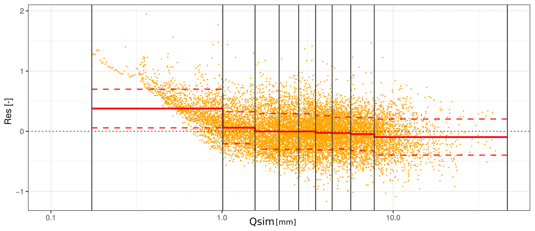
Figure 2 Example of the residual (Res) values computed for Ubaye at Barcelonnette between HydRE and the observations over the calibration period. The vertical lines represent the division of streamflow values in nine classes. The solid (dashed) red lines represent the mean (standard deviation) of all residuals over each class. See Sect. 3.5 for details.

3.5.2 … to a probabilistic methodology

However, the above methodology does account for neither the uncertainty in the observations nor the uncertainty in the simulation. In fact, a part of the ϵ_res[c] could be explained by the uncertainty in observations and in the simulation. As errors in observations and simulations have already been defined (Sect. 3.3.2 and 3.4), their influences can be removed from σ_res[c].

We propose replacing Q_sim by the mean of the simulations, $\stackrel{\mathrm{‾}}{Q_{\mathrm{sim}}}$, in Eq. (2), leading to

$$\begin{array}{}\text{(4)}& \mathit{Res}=\log \left({\displaystyle \frac{Q_{\mathrm{obs}}}{\stackrel{\mathrm{‾}}{Q_{\mathrm{sim}}}}}\right),\end{array}$$

and modifying the error model to account for different uncertainties as follows:

$$\begin{array}{}\text{(5)}& \left\{\begin{array}{l}{\mathit{\mu }}_{\mathrm{model}}\left[c\right]={\mathit{\mu }}_{\mathrm{res}}\left[c\right],\\ {\mathit{\sigma }}_{\mathrm{model}}^{\mathrm{2}}\left[c\right]={\mathit{\sigma }}_{\mathrm{res}}^{\mathrm{2}}\left[c\right]-{\mathit{\sigma }}_{\mathrm{obs}}^{\mathrm{2}}\left[c\right]-{\mathit{\sigma }}_{Q_{\mathrm{sim}}}^{\mathrm{2}}\left[c\right],\end{array}\right.\end{array}$$

with ${\mathit{\sigma }}_{Q_{\mathrm{sim}}}$ being the mean of the standard deviations computed on the ensemble simulated for class c.

3.5.3 Computation

Q_sim simulations in Eqs. (4) and (5) were replaced by the HydRE reconstructions during the calibration period (see Sect. 3.4). If either $\stackrel{\mathrm{‾}}{Q_{\mathrm{HydRE}}}$ or Q_obs is below 0.01 mm d⁻¹, residuals are removed, as Eq. (4) could lead to high values. The definition of σ_obs is similar to the one used in the calibration methodology (see Sect. 3.3.2). Note that since the observation error is only roughly estimated, it is possible to find situations where ${\mathit{\sigma }}_{\mathrm{obs}}\left[c\right]+{\mathit{\sigma }}_{\mathrm{ens}}\left[c\right]>{\mathit{\sigma }}_{\mathrm{res}}\left[c\right]$, but this only happens for 1.9 % of the observations available over the 1973–2006 period. In that case, the value of σ_obs[c] is fixed to 0.01 mm.

3.5.4 Application

The error model defined above is then applied on the HydRE reconstruction. For each day and each member (m) a simulated streamflow, HydRE[m], belongs to class c. Based on the model error, one hundred error values – noted as err – are drawn:

$$\begin{array}{}\text{(6)}& \mathrm{err}\sim \mathcal{N}\left({\mathit{\mu }}_{\mathrm{model}}\right[c],{\mathit{\sigma }}_{\mathrm{model}}[c\left]\right).\end{array}$$

The value of HydRE[m] is then multiplied by the error value:

$$\begin{array}{}\text{(7)}& Q_{{\mathrm{sim}}_{\mathrm{err}}}\left[m\right]=\mathrm{HydRE}\left[m\right]\times \mathrm{err},\end{array}$$

with $Q_{{\mathrm{sim}}_{\mathrm{err}}}\left[m\right]$ being a vector of a length of 100.

Applying this methodology to the 25 members of HydRE leads to an ensemble of 2500 members (25 members × 100 errors). Among those 2500 members, 25 are randomly selected to retrieve a reasonable ensemble size while still characterizing the uncertainty.

To investigate the reduction in the number of members, two sets of simulations – one with all 2500 members and one with only 25 members retained in the final reconstructions – were compared on the three case study catchments (see Sect. 2.1) over the period 1973–2006. A Kolmogorov–Smirnov test was applied to the 25-member and the 2500-member ensembles and confirmed the similarity of the distributions at the 0.05 level for 96.09 % of the time for the Aveyron at Laguépie, 96.17% for the Gave d'Oloron at Sainte-Marie, and 95.22 % for the Ubaye at Barcelonnette.

Finally, the ensemble is reorganized to match the ranks of HydRE in order to preserve the spatio-temporal coherence lost through the random sampling. This method is applied each day over the 1871–2012 period to each of the 661 catchments and leads to a 25-member ensemble daily streamflow reconstruction called HydREM (Hydrological Reconstruction with Error Model).

3.6 Metrics

Several metrics are used to compare the different reconstructions. The continuous ranked probability score (CRPS; Brown, 1974) is a commonly used score for ensemble verification and is defined as follows:

$$\begin{array}{}\text{(8)}& \mathrm{CRPS}[x,y]={\displaystyle \frac{\mathrm{1}}{M}}\sum _{i=\mathrm{1}}^M\underset{-\mathrm{\infty }}{\overset{\mathrm{\infty }}{\int }}\left[F\right(x)-H(y){]}^{\mathrm{2}}\mathrm{d}x,\end{array}$$

with x being the ensemble to be evaluated, y the observation, F the cumulative distribution function, M the number of observations, and H the Heaviside function. The decomposition of the CRPS (Hersbach, 2000) is also computed to study the reliability part and the potential CRPS. As explained in Hersbach (2000), the reliability (Reli) gives an information similar to the rank histogram, and the potential CRPS (Pot) is linked to the spread of the ensemble – the uncertainty – and to the number of outliers.

$$\begin{array}{}\text{(9)}& \mathrm{CRPS}=\mathrm{Reli}+\mathrm{Pot}\end{array}$$

The optimal value of the CRPS and its decomposition is therefore zero. Furthermore, in order to compare between the different catchments, the CRPS and its decomposition are normalized by the average streamflow over the 1973–2006 period. The normalized version of the scores is denoted with an N at the beginning (NCRPS, NPot, NReli) and are expressed in percentages of the average streamflow.

In addition, the KGE (Gupta et al., 2009) and its decomposition were used to provide a more insightful description of the datasets. The KGE is defined as follows:

$$\begin{array}{}\text{(10)}& \mathrm{KGE}[x,y]=\mathrm{1}-\sqrt{(r-\mathrm{1}{)}^{\mathrm{2}}+(\mathit{\alpha }-\mathrm{1}{)}^{\mathrm{2}}+(\mathit{\beta }-\mathrm{1}{)}^{\mathrm{2}}},\end{array}$$

where r is the linear correlation coefficient, α the ratio of variance, and β the ratio of means. Contrary to the CRPS, the optimal value of the KGE is 1 when the two vectors, x and y, match up perfectly. KGE is computed for each ensemble member, and median values over each ensemble are retained.

4 Results

This section presents an intercomparison of the two reconstructions developed here (HydRE and HydREM) and other products referred to in the previous sections: Safran Hydro (Sect. 2.2), SCOPE Hydro (Sect. 2.3), and GRUN (Sect. 2.4). Such an intercomparison is performed regarding various aspects: (1) a daily time series example from three case study catchments; (2) a comprehensive validation against observations over 1960–2012; (3) a validation against the few long-term observations over 1920–2012; (4) an assessment of multidecadal variations over the four main French basins, (5) a long-term evolution of high-flow and low-flow events at the monthly scale; and, lastly, (6) the example of an extreme flood event in 1890.

4.1 Time series example

A first assessment of the reconstructions is conducted through a daily time series analysis of the year 1920 for the three case study stations (Fig. 3). This year is chosen to reflect the behaviour of the hydrological reconstructions in the distant past and because streamflow observations are available over the three stations.

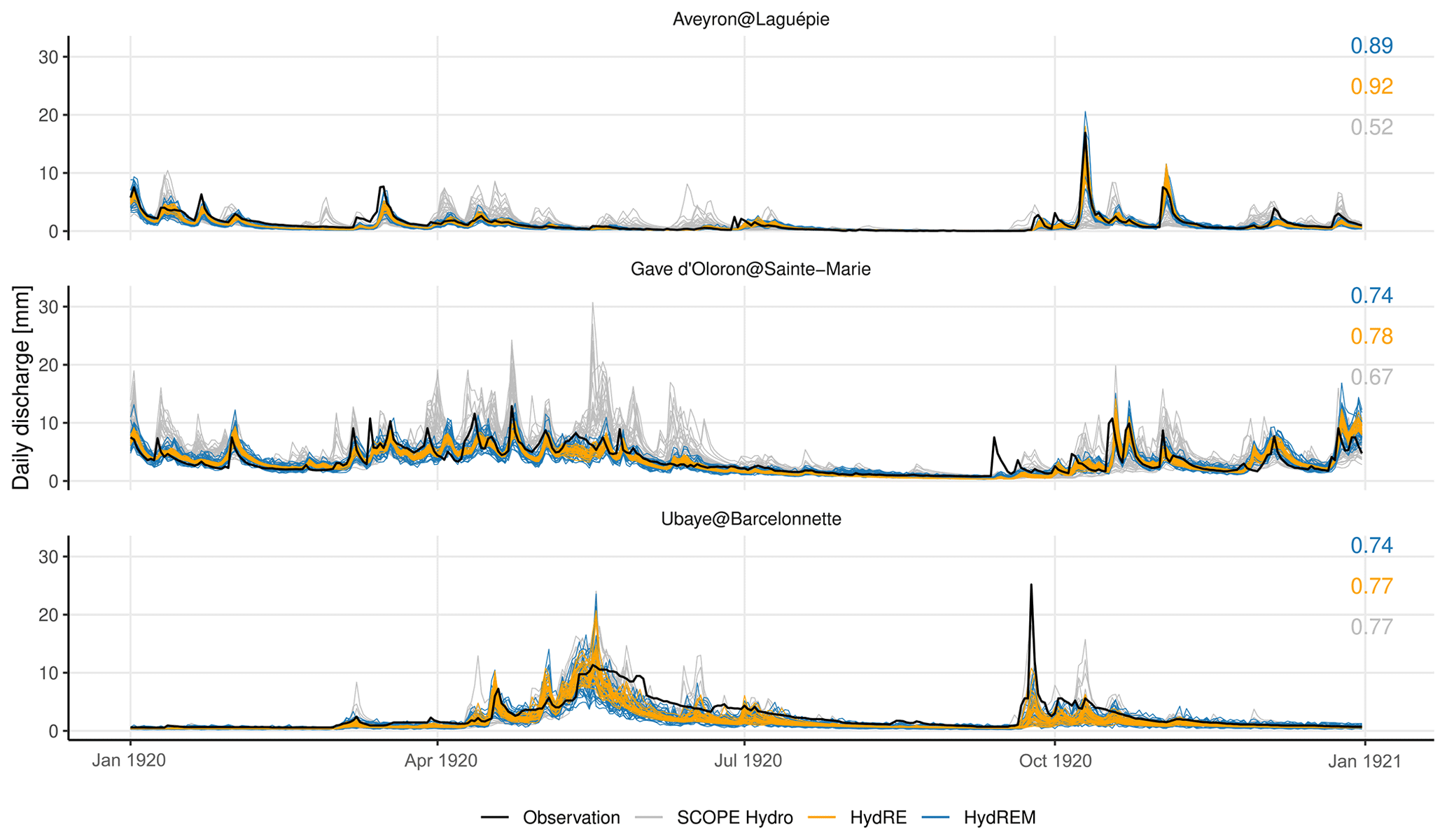
Figure 3 Daily time series over the three case study catchments during the year 1920. The values in the top-right corner indicate the median of the 25 correlations between the observation and the 25-member ensemble.

For SCOPE Hydro, the relatively high uncertainty reflects the high uncertainty in SCOPE Climate – the corresponding meteorological input – as information only comes from a large-scale reanalysis. The uncertainty in HydRE is clearly lower as FYRE Climate used in situ observations to reduce the uncertainty in the reanalysis. Finally, the HydREM uncertainty depends on not only the quality of FYRE Climate but also the ability of GR6J to reproduce the hydrological behaviour of the catchment. For Ubaye, the basin is influenced by snowmelt, which is quite difficult to reproduce, and the quality of the observations in 1920 is possibly flawed due to the management of small upstream dams, as shown by the recession, which seems unrealistic for some days. In any case, even while accounting for the modelling error, HydREM seems to have a lower uncertainty than SCOPE Hydro for Gave d'Oloron at Sainte−Marie and Aveyron at Laguépie. The ensemble of HydRE seems to be underdispersed, but this is not the case once the modelling error from Sect. 3.5 is applied, i.e in HydREM reconstructions. The added values of HydRE and HydREM, in comparison to SCOPE Hydro, in Gave d'Oleron at Sainte−Marie and Aveyron at Laguépie are clearly visible in terms of correlation with the observations. However, for Ubaye at Barcelonnette, it is more difficult to find which of the reconstructions reproduces the observations better.

The time series of the three case study catchments are now investigated at a yearly time step (Fig. 4). Over the 1960–2012 period, HydRE and HydREM show a higher correlation with observations than SCOPE Hydro. Furthermore, the uncertainty is lower in HydRE and HydREM than in SCOPE Hydro. HydRE and HydREM display a behaviour similar to Safran Hydro. However, the absence of uncertainty in Safran Hydro makes it difficult to compare to ensemble reconstructions. Before 1960, HydRE and HydREM still have a higher correlation with the observations than SCOPE Hydro. However, for Aveyron at Laguépie before 1940, a dry bias, which is not present in SCOPE Hydro, seems to appear in HydRE and HydREM. This could reflect a dry bias in the FYRE Climate reanalysis as it affects both HydRE and HydREM.

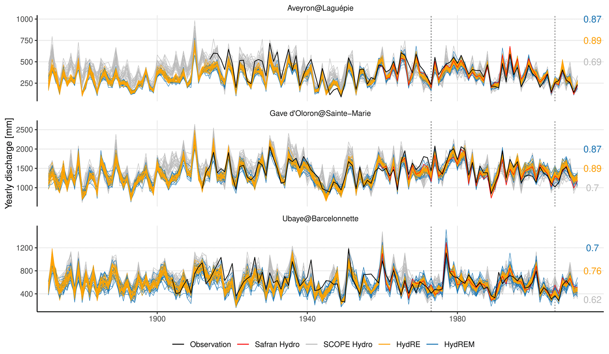
Figure 4 Yearly time series over the three case study catchments between 1871 and 2012. The values in the top-right corner indicate the median of the 25 correlations between the observation and the 25-member ensemble.

4.2 Validation against observations between 1960 and 2012

The performance of the different reconstructions is evaluated with the KGE during the calibration period 1973–2006 (Fig. 5). SCOPE Hydro reconstruction shows the lowest KGE, which could be explained by the fact that (1) the reconstruction uses parameters calibrated with Safran and not SCOPE Climate and (2) the meteorological forcing information comes only from a large-scale reanalysis. KGE values of Safran Hydro and HydRE are quite close, with some catchments showing slightly lower values in HydRE. This could be explained by the fact that HydRE values are median values over all 25 members. For HydREM, KGE values are slightly lower than in Safran and HydRE due to the application of random sampling and the increasing uncertainty when the error model is applied.

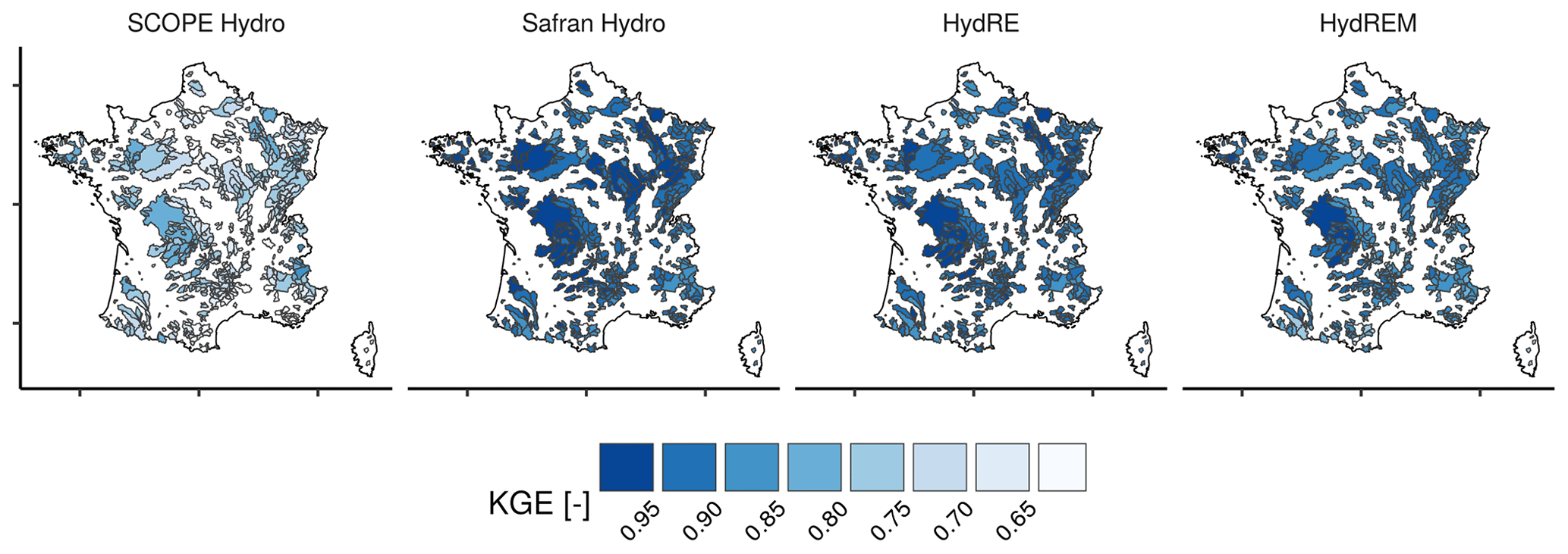
Figure 5 Map of the KGE$\left(\sqrt{Q}\right)$ computed during the calibration period, 1973–2006, for different hydrological reconstructions. For SCOPE Hydro, HydRE, and HydREM, the score is computed as the median of 25 member values.

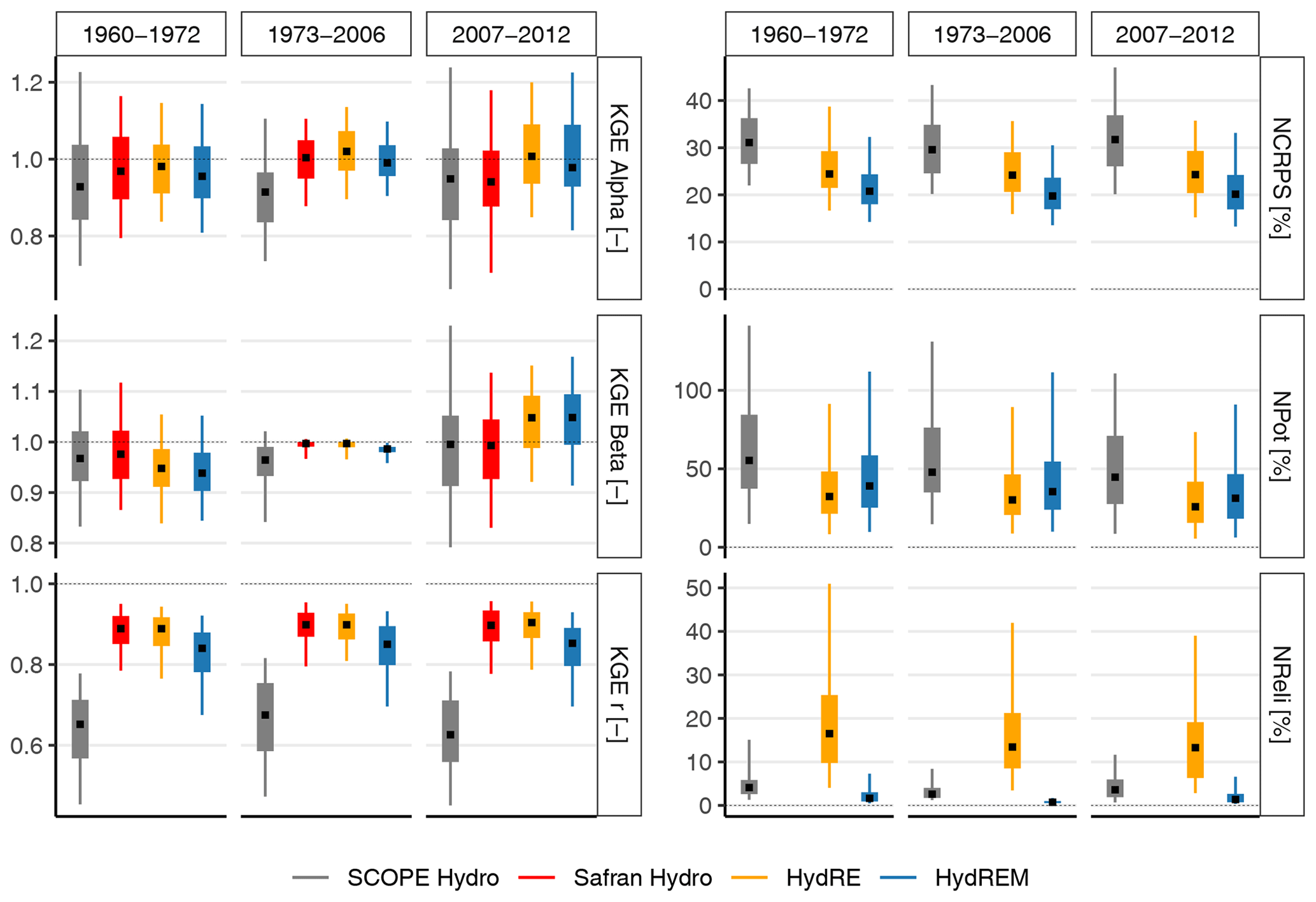
Figure 6 Boxplot of different metrics over three distinct periods using 173 stations. For SCOPE Hydro, HydRE, and HydREM, the score displayed is computed as the median of 25 member metrics. The squares correspond to the median, the thick lines to the 25th and 75th quantiles and the narrow lines to the 5th and 95th quantiles. The dotted black lines represent the optimal values for each metric.

To go further into the comparison over 1960–2012, we compute different metrics over three sub-periods: 1960–1972, 1973–2006, and 2007–2012. Metrics are computed only on 173 stations, i.e. the ones with observations available over the entire 1960–2012 period.

The decomposition of the KGE over the three sub-periods is shown in the left panel of Fig. 6. Globally, the values of the KGE α – the variability component – and KGE r – the correlation component – do not differ largely, and the hierarchy between the different reconstructions is maintained over the different time periods. However, for the KGE β – the bias component – the values are closer to zero during the calibration period, except for SCOPE Hydro, as it uses parameters calibrated with Safran. HydRE and HydREM exhibit a slight bias (±5 %) outside the calibration period contrary to Safran Hydro. Overall, the KGEs of SCOPE Hydro are sub-optimal in comparison to the other reconstructions. Safran Hydro, HydRE and HydREM show almost similar values, except for KGE r, for which HydREM displays slightly lower values.

The decomposition of the CRPS is also explored in the right panel of Fig. 6. Note that it is not possible to compute the CRPS for the deterministic Safran Hydro reconstruction. As for the KGE, the hierarchy between the reconstructions is relatively stable over the three sub-periods for the different metrics. The NCRPS – the total CRPS relative to the mean streamflow over the calibration period – shows the advantage of using FYRE Climate as input, with lower values for HydRE and HydREM than for SCOPE Hydro. Applying the error model also brings an improvement, although smaller, with lower values in HydREM. The NPot – part of the CRPS representing the accuracy – shows similar values between HydRE and HydREM while showing no added value of the error model but lower values than SCOPE Hydro. On the contrary, the NReli – related to the reliability of the ensemble – shows an underdispersion of the HydRE ensemble, with values much larger than for SCOPE Hydro or HydREM. Applying the error model leads to a quite low (< 5 %) NReli of HydREM and below the one of SCOPE Hydro.

The study considering different time periods through the decomposition of KGE and CRPS shows the stability of HydRE and HydREM during the 1960–2012 period, with results (1) close to Safran Hydro, (2) better than SCOPE Hydro, and (3) with a correct definition of the uncertainty for HydREM. However, it also shows a small bias outside the calibration period.

4.3 Validation against long-term observations over 1920–2012

This subsection looks further into the past in order to assess the quality of the hydrological reconstructions over the 1920–2012 period. Unfortunately, before the 1970s, the number of stations with continuous measurements decreases drastically. Therefore, the 20 stations with the longest record of continuous observations, among the 661 near-natural catchments where discharge was simulated, were selected here. While this set of 20 stations does not cover the entire hydroclimatic context in France – they are mainly located in the south and in mountainous area (see Fig. 1) – it allows for a characterization over a long time period. The daily CRPS and its decomposition, as well as the KGE components, were computed for each year of the 1920–2012 period. This is done for each station, and for deterministic metrics, we compute the median values over the ensembles. Finally, the average value over the 20 stations is computed and shown in Fig. 7.

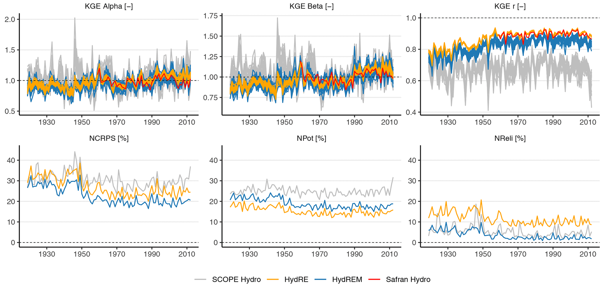
Figure 7 Evolution of metrics averaged over a set of 20 stations for the 1920–2012 period. For SCOPE Hydro, HydRE, and HydREM, the score is computed as the median of 25 member values. The dotted black lines represent the optimal values for each metric. The NCRPS, NPot and NReli correspond, respectively, to the CRPS, Pot, and Reli normalized by the average discharge at each station.

As in Sect. 4.2, the CRPS decomposition shows the importance of HydRE and HydREM in terms of CRPS (NCRPS) and potential CRPS (NPot) in comparison to SCOPE Hydro. However, the reliability (NReli) of HydRE is higher than the ones in SCOPE Hydro and HydREM. Over time, both the potential CRPS and the reliability first show a plateau between 1920 and 1950, then a decrease over the 1950s and 1960s, and a new plateau until 2012. The transition period matches a strong increase in the number of weather stations used in FYRE Climate (Devers et al., 2021). However, as this is also visible (although much less) in SCOPE Hydro, this could be linked to another origin; see Sect. 5.

SCOPE Hydro displays the KGE β as being close to zero over the entire period but with a high dispersion. The KGE β of HydRE and HydREM is highly similar, with a small bias [±5 %] during the 1960–2012 period and a dry bias centred around −10 % over the 1920–1950 period. Note that this is also the period identified in Sect. 4.1 at Aveyron at Laguépie. The KGE α shows a behaviour similar to KGE β, with a high dispersion in SCOPE Hydro and good results for HydRE and HydREM but a variability that is lower in HydRE and HydREM than in the observations over 1920–1950. This could possibly explain the bias appearing at the same time, as underestimating variability could lead to an underestimation of peak streamflow playing an important role in yearly-averaged streamflow. For KGE r, even if HydREM displays slightly lower correlations than HydRE, their values are always above the ones in SCOPE Hydro, even at the beginning of the period. For HydRE and HydREM, a strong evolution is linked to the number of observation assimilated in FYRE Climate (Devers et al., 2021).

As a summary, even if a small dry bias seems to appear before the 1950s, the HydREM reconstruction shows the added values of both using a reanalysis as meteorological input and a model error.

4.4 Multidecadal variations over large catchments

In order to further describe HydRE and HydREM, multidecadal variations in the reconstruction are compared to the ones in SCOPE Hydro, in the observations over the four main rivers of France (see Sect. 2.1), and in the GRUN dataset (see Sect. 2.4). As those products have different spatial and temporal resolutions, the following transformations are first applied:

• For SCOPE Hydro, HydRE, and HydREM, yearly anomalies are first computed over 1871–2012 with respect to the 1970–2000 period for each of the 25 members and for the 661 catchments. Each simulated catchment is then assigned to one of the main rivers (see Fig. 1). Finally, for each member and main river, the mean of all catchment anomalies is computed.

• For GRUN, yearly anomalies over 1871–2012 with respect to the 1970–2000 period are computed for each grid cell over France for each of the 50 members. Each cell is then assigned to a main river based on its location (see Sect. 2.4 for the number of cells by catchment). As previously, for each member and main river, the average of grid cell anomalies is computed.

• For the observations, yearly anomalies over 1871–2012 with respect to the 1970–2000 period are simply computed for the four main rivers.

Finally, a 30-year centred rolling mean is applied to each time series of anomalies to highlight multidecadal variations.

Results are presented in Fig. 8. First, applying the error model does not affect multidecadal variations as HydRE and HydREM display similar ones, even if the dispersion is different. Overall, the GRUN dataset is closer to the HydRE and HydREM reconstructions than to SCOPE Hydro, especially before 1940, except for Loire at Montjean. Indeed, during the 1900–1940 period, SCOPE Hydro shows strong positive anomalies which are not shown by HydRE, HydREM, or GRUN.

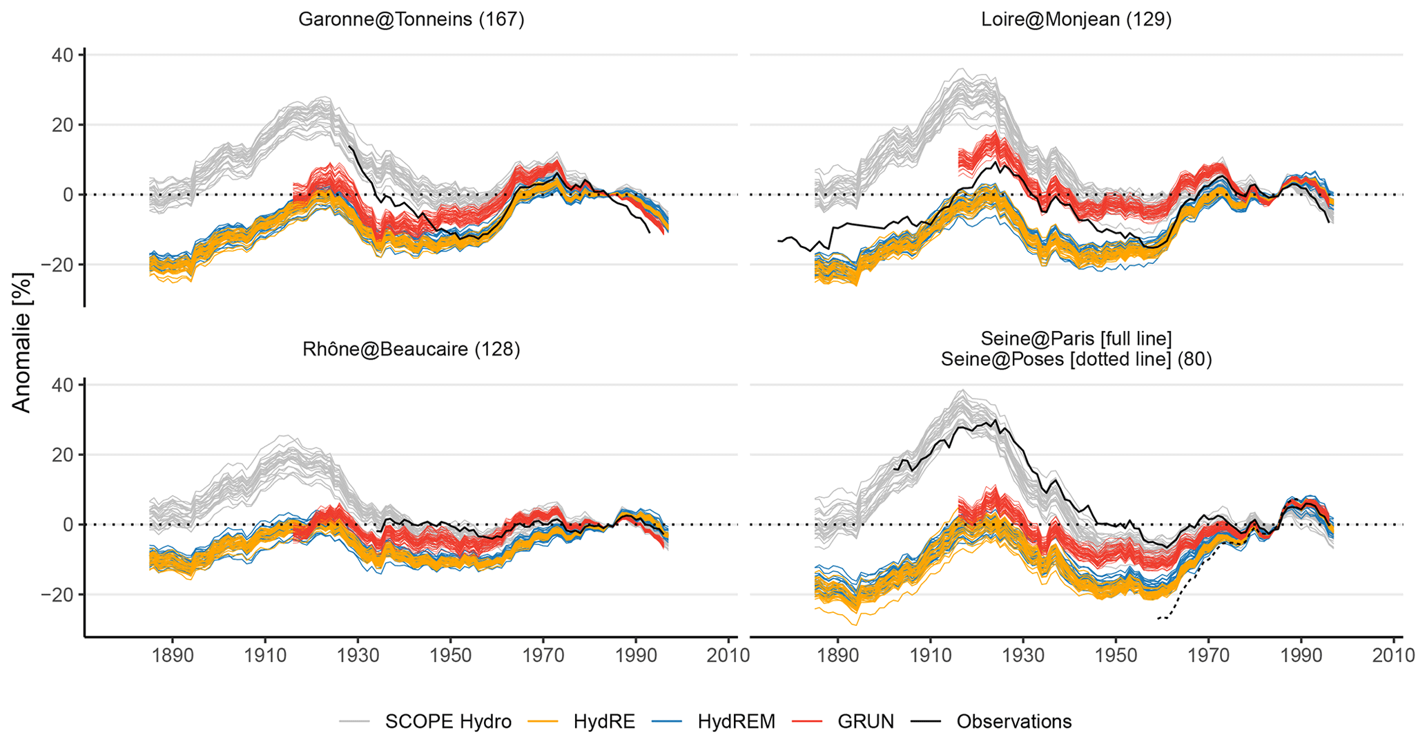
Figure 8 Multidecadal variations in different reconstructions over the four main catchments of France and comparison with available observation records. The number in brackets indicates the number of stations modelled in this catchment. See text for details.

Concerning Garonne at Tonneins, the observations are closer to SCOPE Hydro than HydRE, HydREM, or GRUN before 1950. For Rhône at Beaucaire, multidecadal variations in the observations are lower than in the different reconstructions, with GRUN included. This could reflect the strong anthropogenic modifications of the Rhône catchment. For Seine at Poses, HydRE and HydREM are closer to the observations than SCOPE Hydro or GRUN over 1950–2012, but the time series is rather short. For Seine at Paris, the observations are quite coherent with SCOPE Hydro over the whole period. The other reconstructions do not provide coherent multidecadal variations. However, the catchments used to compare the variations in the reconstructions cover a larger area than that of the Seine at Paris catchment. Lastly, for Loire at Montjean, the GRUN dataset seems to better represent observed variations. Indeed, over the 1920–1940 period, a overestimation is seen in SCOPE Hydro, whereas HydRE and HydREM underestimate anomalies. However, this tendency is almost null over 1890–1920, whereas it still present in SCOPE Hydro.

Globally, all hydrological reconstructions have difficulties in representing the multidecadal variations present in the discharge observations. There are probably multiple sources of these discrepancies, and they are difficult to quantify, but several have been identified: (1) observations from the distant past could be erroneous, and the change in the system measurement could lead to strong inhomogeneities (Kuentz et al., 2015); (2) the hydrological model could have difficulties in simulating the multidecadal variability, but the discrepancies appear both in the reconstructions GRUN produced by a random forest algorithm and those SCOPE Hydro/HydRE/HydREM produced by a conceptual hydrological model; (3) the hydrological models do not provide a discharge simulation at the hydrological station of the four main rivers, and the time series are aggregated over a large catchment and the anomalies are calculated subsequently; and (4) HydRE and HydREM, as suggested by Fig. 7, are affected by a dry bias before the 1940s that leads to a rising trend in the anomalies (for SCOPE Hydro, the inverse is visible).

4.5 Evolution of monthly high-flow and low-flow events over the 1871–2012 period

Figure 9 allows us to grasp the evolution of the number of stations with at least one monthly streamflow above (below) the 99.9 % (0.1 %) monthly quantile during a year.

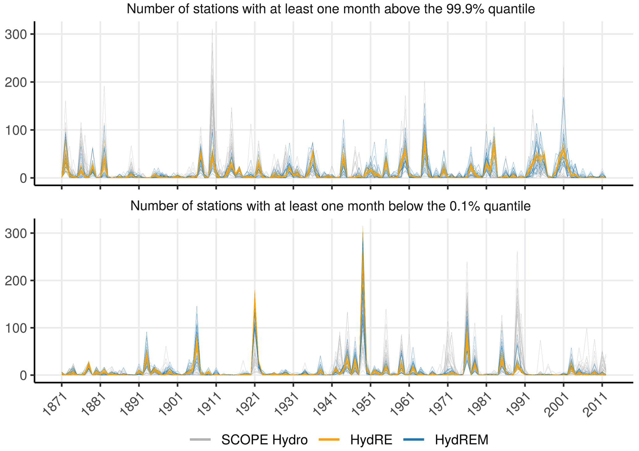
Figure 9 Evolution of the number of stations with at least one monthly streamflow above (below) the 99.9 % (0.1 %) monthly quantile during a year. This is applied separately for each of the 25 members, and the period of reference used to compute the quantiles is 1871–2012.

For high flows (Fig. 9, top panel), the methodology highlights different years with a large number of stations that have monthly values above the 99.9 % quantile, among them 1872, 1876, 1882, 1907, 1910, 1935–1936, 1944–1945, 1954–1955, 1960–1961, 1966, 1993–1994, and 2001. The frequency of events does not seem to follow a clear trend, but the 1885–1905 period shows quite a low number of stations. It is important to note that all the years mentioned above are consistent with the ones available in Les inondations remarquables en France (Lang and Coeur, 2014, Remarkable Floods in France), which provides a thorough review of floods over the 1770–2011 period based on archive evidence.

Furthermore, one can also find some interesting references to those years in other literature sources and even paintings:

• winter 1872–1873 with the Seine flood, as testified in Alfred Sisley's painting Le Bac de l'île de la loge, inondation (The ferry of loge island, flooding);

• the first months of 1910 are also largely documented in Lang and Coeur (2014), with flood occurring in the northern half of France;

• the end of 1935 is also mentioned (Pardé, 1937; Lang and Coeur, 2014), with flooding of the Seine and the Rhône rivers;

• winter 1954–1955 is also present, with several instances of flooding of not only the Rhône River (Pardé, 1958) but also the Seine River (Lang and Coeur, 2014). Furthermore, a slow flood also hit the Saône River, leading to a up to 6 km wide river in some places (Dubrion, 2008).

Among the years with a relatively high number of stations with low-flows (Fig. 9, bottom panel), the year 1893 was already identified in Ireland and in the UK by Cook et al. (2015). The year 1906 allows us to identify the well-known meteorological drought identified by Plumandon (1907). The 1921 drought event (Duband, 2010) is also well seen in the HydREM dataset, with a large temporal extent. Another long drought is seen around the year 1949, which is also mentioned for the Loire catchment (Moreau, 2004). Finally, the droughts of 1976; 1985; 1990; and, more recently, 2003 are consistent with observation time series, showing record-breaking minimums for these years.

It is interesting to note that most of the events are captured in both SCOPE Hydro and HydRE/HydREM. This is actually not surprising given the monthly time step. Indeed, the added value of HydRE and HydREM comes from the assimilation of daily meteorological values in their input, i.e. with FYRE Climate. Still, some events seem more or less important when looking at SCOPE Hydro or HydRE/HydREM, e.g. high flows in 1910 and low flows in 1971 and 1990.

The study of the high-flow and low-flow records in HydRE and HydREM reconstructions shows the importance of such datasets to better apprehend extremes of the past and a good coherence with other indirect data sources.

4.6 Example of an extreme flood event

At the end of September 1890, an extreme rainfall event in the Cévennes area in southern France (http://pluiesextremes.meteo.fr/france-metropole/Inondations-en-Cevennes-Crue-historique-de-l-Ardeche.html, last access: 21 February 2022) led to a record flood over the Ardèche River between 21 and 23 September 1890 (Sheffer et al., 2003; Naulet et al., 2005). Daily streamflow between 20 and 25 September was transformed into quantiles with respect to the entire 1871–2012 period independently for each reconstruction dataset (SCOPE Hydro, HydRE, and HydREM) and each member. The means of the 25 quantiles – one for each member – are displayed in Fig. 10. Only a few observations are available in the Cévennes, and the stations are located in the east part of the region, where the event was less important. We choose not to display those observations because the short period of observation does not allow us to compute long-term quantiles such as those used in the reconstructions.

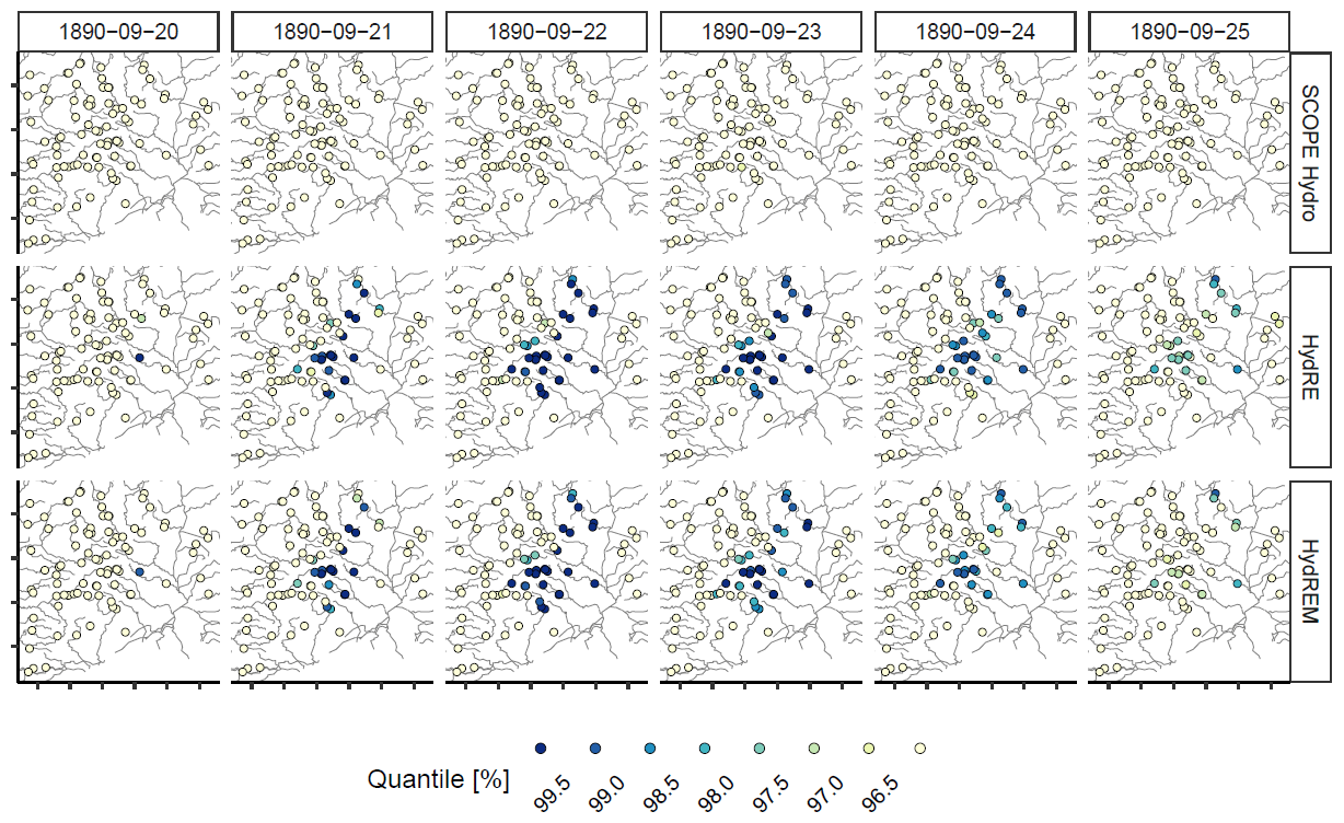
Figure 10 Map of the mean quantiles relative to daily streamflow in the reconstructions over the Cévennes area over 5 d in September 1980.

SCOPE Hydro first demonstrates low-quantile values over all catchments compared to HydRE/HydREM. Indeed, only a few members in SCOPE Hydro display high values (not shown), but this does not affect the mean of the ensemble. The mean values in HydRE and HydREM are more consistent with the studies mentioned above than the one in SCOPE Hydro given the exceptional nature of the event. Furthermore, HydRE and HydREM show a spatial structure consistent with the events usually observed in the Cévennes area, with very high values on a small number of catchments. Finally, the difference between HydRE and HydREM on some catchments shows the sensitivity of the model error regarding the high-range streamflow simulated.

5 Discussion

5.1 Stability over time

The modelling framework used to produce both HydRE and HydREM is subject to strong assumptions in terms of stability over time.

First, the calibration of the hydrological model on a long but still limited period follows the hypothesis that the link between meteorological and hydrological variables is well captured – even in extrapolation with different hydroclimatic conditions – and that this link is stable over time through a temporal transferability of parameters. Over long periods, such as the one considered here, this assumption could be questionable, especially if the calibration is made during a wet or dry period. In our case, even if the calibration is made over 26 years, it seems that, at least for the Seine catchment, a wet phase is present during the whole calibration period (see Fig. 8; Boé and Habets, 2014; Bonnet et al., 2020). A longer calibration period could lead to several hydrological differences, and a solution could be to use the whole period of availability of the observation instead of being limited to 1973–2006. In this regard, some methods could have been used to quantify not only the sensitivity of the calibration to the period, such as the classic split-sample test (Klemeš, 1986), but also new methods testing the validity of these assumptions. Two examples are the generalized split-sample test (Coron et al., 2012), which uses calibration–validation periods with a 10-year sliding window, and the robustness assessment test (Nicolle et al., 2021), which assesses potential undesirable dependencies of hydrological model performance on climate variables.

Secondly, the stability of the reconstructions also depends on the stability of the input data. For HydRE and HydREM, FYRE Climate is used to force the GR6J model. This reanalysis is a combination of SCOPE Climate and in situ measurements of precipitation and temperature. Then, some sources of instability can potentially be present: (1) the SCOPE Climate dataset is driven by the 20th Century Reanalysis, which may include some trend inconsistencies (Krueger et al., 2013); (2) the SCOPE climate used a bias correction of precipitation based on the 1958–2008 period as reference (Caillouet et al., 2019) that could not be stable over time; and (3) the assimilation of station measurements in FYRE Climate could also lead to temporal inconsistencies due to the evolution of the observation network and of its quality.

5.2 Uncertainty in the modelling/calibration framework

The modelling framework of this study includes several types of uncertainty: (1) the measurement uncertainty during calibration and model error definition; (2) the uncertainty in the input meteorological variables during calibration, simulation, and model error definition; and (3) the modelling uncertainty in HydREM. In order to characterize and account for these uncertainties, we used both a Monte Carlo approach – with the hypothesis that the uncertainty in these variables can be represented by an ensemble – during the calibration and simulation and a representation of the errors by a distribution during the application and definition of the error model.

To account for these uncertainties, there are several methods, including the GLUE methodology (Smith et al., 2019) and the Bayesian approach (Renard et al., 2010). The first one tries to capture all the uncertainty using a large number of parameter sets, and only a few are retained based on the quality of the reconstruction during a recent period. The second also attempts to quantify the total forecast uncertainty but by defining input and structural components. While our approach is closer to the Bayesian approach, it clearly differs because no inference is defined between the input and structural components.

Hence, a logical path for improving the modelling framework proposed here would be to apply a proper Bayesian methodology, such as the one proposed by Renard et al. (2010).

5.3 Definition of the error model

Concerning the error model, a previously developed postprocessing approach has been applied, with some modifications, to match the ensemble context (see Sect. 3.5). In this updated version as well as in the original one, some hypotheses need to be discussed. First, the original approach relies on the assumption that residuals errors (i.e. the ratio of observed streamflow over simulated streamflow) follow a log-normal distribution inside each class defined. This hypothesis allows us to transform residuals through a log transformation to obtain a Gaussian distribution defined only by the mean and standard deviation of the residuals. This hypothesis was verified here through histogram checks (not shown here), but this hypothesis could be confirmed using the Shapiro–Wilk test (Shapiro and Wilk, 1965). Secondly, errors in the HydRE ensemble and measurements are here assumed to follow a Gaussian distribution, which is a strong assumption, especially for the observations. It could therefore not be that appropriate to remove the uncertainty in HydRE or the observations from the error model (see Eq. 5). Finally, the definition of the model error over a given period (here equal to the calibration period) contains the same assumptions as mentioned in Sect. 5.1. It should be noted that a multi-model approach could have been implemented to define the model error (Arsenault et al., 2015; Thébault et al., 2024).

5.4 On the validation of hydrological and climate data

The validation of HydRE and HydREM was done here through different periods, timescales, and spatial scales and using both observations and other available reconstructions. Still, in the distant past – in our case before 1920 – the validation of the reconstructions is made difficult by the lack of data over a large number of catchments. Finally, a further validation of the HydRE and HydREM could use other hydrological reconstructions covering the 1900–2005 period (Bonnet et al., 2017, 2020). However, those reconstructions provide only streamflow over catchments larger that the ones considered here.

Besides, the reconstructions produced here allow us to learn more about the strengths and weaknesses of the FYRE Climate reanalysis used as input. Indeed, as the quality of the hydrological reconstruction strongly depends on the quality of the input (Caillouet et al., 2017; Raimonet et al., 2017; Smith et al., 2019), the hydrological modelling provides an independent validation of FYRE Climate. Thus, this paper shows that FYRE Climate provides a good representation of dry/wet extreme events over the entire 1871–2012 period. Furthermore, the reconstruction of precipitation appears to be better than in previous products – such as SCOPE Climate – leading to a better correlation in terms of discharge. However, the results also suggest a probable dry bias in the FYRE Climate precipitation before 1940.

6 Conclusions

The present study provides long-term reconstructions of daily streamflow over a set of 661 near-natural catchments. Their creation is based on the new FYRE Climate reanalysis (Devers et al., 2021) for temperature and precipitation, the SCOPE Climate reconstruction (Caillouet et al., 2019) for evapotranspiration, and the GR6J lumped continuous rainfall–runoff model (Pushpalatha, 2013). Furthermore, an effort has been made to take various sources of uncertainty into account in the calibration and simulation framework, including uncertainties in the input, streamflow measurement, and hydrological model. The two resulting 25-member ensemble reconstructions, namely HydRE and HydREM, span the 1871–2012 period at a daily timescale.

In Sect. 4.2, HydrRE and HydREM were first compared to existing hydrological reconstructions, SCOPE Hydro and Safran Hydro (Caillouet et al., 2017), using dependent and independent streamflow measurements over the recent period. The newly produced reconstructions show a stronger correspondence with observations than SCOPE Hydro and a similar one with respect to Safran Hydro. Safran Hydro, however, spans only the 1958–2012 period and does not provide any information about the associated uncertainty. Overall, the quality of the HydRE and HydREM reconstructions are close to one another, but applying the error model leads to a higher reliability. Section 4.3 pushes the validation further using a set of 20 stations with observations available over the 1920–2012 period. HydRE and HydREM reproduce observed streamflow over the entire period better than SCOPE Hydro. Once again, HydREM shows a better reliability than HydRE. Finally, the variability at the annual timescale of HydRE and HydREM is closer to the observations than SCOPE Hydro, but before 1950, a slight dry bias seems to be present.

The study of multidecadal variations in Sect. 4.4 over the four main rivers of France has put forward the large differences between SCOPE Hydro and HydRE/HydREM. The latter two show a better agreement with the GRUN reconstructions over the 1915–2000 period but with rather large differences from one basin to another. Lastly, the reconstructions were compared over a small set of catchments located in the Cévennes area during a well-documented flood event in 1890. HydRE and HydREM provide higher streamflow values than SCOPE Hydro, showing the importance of those two datasets for studying extreme events.

The varying results of these study have put forward the importance of both HydRE and HydREM when comparing them to other existing datasets. Those two 25-member reconstructions make daily streamflow over 661 near-natural catchments of France between 1 January 1871 and 29 December 2012 available. For both, the 25-member ensemble spread reflects the uncertainty in the reconstructed streamflow. A preference should be given to HydREM, as results have put forward its higher reliability. However, as the two products show good results in reproducing observations, long-term variations, and flood events, we choose to provide both through two joined datasets: HydRE (Devers et al., 2023a) and HydREM (Devers et al., 2023b).