the Creative Commons Attribution 4.0 License.
the Creative Commons Attribution 4.0 License.
 | 04 Jul 2024
A national-scale hybrid model for enhanced streamflow estimation – consolidating a physically based hydrological model with long short-term memory (LSTM) networks
Julian Koch
Simon Stisen
Lars Troldborg
Raphael J. M. Schneider
Accurate streamflow estimation is essential for effective water resource management and adapting to extreme events in the face of changing climate conditions. Hydrological models have been the conventional approach for streamflow interpolation and extrapolation in time and space for the past few decades. However, their large-scale applications have encountered challenges, including issues related to efficiency, complex parameterization, and constrained performance. Deep learning methods, such as long short-term memory (LSTM) networks, have emerged as a promising and efficient approach for large-scale streamflow estimation. In this study, we have conducted a series of experiments to identify optimal hybrid modeling schemes to consolidate physically based models with LSTM aimed at enhancing streamflow estimation in Denmark.
The results show that the hybrid modeling schemes outperformed the Danish National Water Resources Model (DKM) in both gauged and ungauged basins. While the standalone LSTM rainfall–runoff model outperformed DKM in many basins, it faced challenges when predicting the streamflow in groundwater-dependent catchments. A serial hybrid modeling scheme (LSTM-q), which used DKM outputs and climate forcings as dynamic inputs for LSTM training, demonstrated higher performance. LSTM-q improved the mean Nash–Sutcliffe efficiency (NSE) by 0.22 in gauged basins and 0.12 in ungauged basins compared to DKM. Similar accuracy improvements were achieved with alternative hybrid schemes, i.e., by predicting the residuals between DKM-simulated streamflow and observations using LSTM. Moreover, the developed hybrid models enhanced the accuracy of extreme events, which encourages the integration of hybrid models within an operational forecasting framework. This study highlights the advantages of synergizing existing physically based hydrological models (PBMs) with LSTM models, and the proposed hybrid schemes hold the potential to achieve high-quality large-scale streamflow estimations.
- Article
(8960 KB) - Full-text XML
- BibTeX
- EndNote


Accurate streamflow estimates are essential for sustainable water resource management, prediction of extreme events, energy production, decision-making, and the protection of both human populations and natural ecosystems (Devitt et al., 2023; Hoy, 2017; Satoh et al., 2022). Collecting spatiotemporally adequate streamflow data through observations can be challenging. Therefore, various conceptual and process-based hydrological models have been developed and applied for streamflow interpolation and extrapolation in time and space, such as supplementing the missing streamflow at stations, transferring the parameters to basins showing high hydrological similarities, and predicting the streamflow under future conditions (Beven, 1996, 2020; Devia et al., 2015). These models are based on a priori knowledge and physical principles to simulate critical hydrological processes, e.g., infiltration, evapotranspiration (ET), runoff routing, and groundwater movement, and have been widely and successfully used across domains and scales.
Physically based hydrological models (PBMs) stand out among those diverse hydrological models and have been widely used in recent decades due to their sophisticated structures and advanced parameterizations (Devia et al., 2015; Fatichi et al., 2016; Pakoksung and Takagi, 2021; Refsgaard et al., 2022). These features enable PBMs to simulate complex hydrological processes and facilitate a detailed analysis at high spatiotemporal resolutions. However, PBMs are susceptible to biases arising from inadequate inputs, suboptimal structural design, or improper parameterization schemes (Herrera et al., 2022; Dembélé et al., 2020; Silvestro et al., 2015; Koch et al., 2016). Therefore, the streamflow performance of PBMs is not always satisfactory for practical applications and may not consistently outperform simpler lumped and conceptual hydrological models. For example, some studies have pointed out that PBMs encounter difficulties in capturing peak flows (Baroni et al., 2019; Kumari et al., 2021; Moges et al., 2021; Sahraei et al., 2020).
The Danish Water Resources Model (DKM) is an example of a PBM (Højberg et al., 2009) and is based on the distributed, integrated model code MIKE SHE (DHI, 2020). The DKM has been calibrated against a large dataset of groundwater head observations and streamflow measurements utilizing dense national monitoring networks (Henriksen et al., 2021; Stisen et al., 2020). Streamflow performance is considered satisfactory, with an average Kling–Gupta efficiency (KGE) of 0.75, though performance varies both temporally and spatially. Overall, the DKM tends to exhibit better performance in basins with larger drainage areas compared to smaller ones (Henriksen et al., 2021). In recent years, several projects related to hydrological monitoring, national flood warning, and nitrate modeling have emerged that rely on DKM-simulated streamflow time series (Henriksen et al., 2023). Therefore, enhancing the accuracy of DKM simulations using advanced methods, such as deep learning (DL) algorithms, is deemed necessary and will have far-reaching implications for a range of applications.
Data-driven techniques are well suited for capturing patterns and relationships within the data without relying on prior assumptions or models (Kawaguchi et al., 2022; Ke et al., 2017; Wu et al., 2022). The runoff process is intricately connected to climate records and other processes in the water cycle. These relationships can be learned through data-driven methods, such as LSTM (Wi and Steinschneider, 2024; Wang et al., 2023; Kratzert et al., 2018). LSTM is a type of recurrent neural network proficient in handling time series data and has proven to effectively capture the variations and dependencies within sequential data (Hochreiter and Schmidhuber, 1997; Greff et al., 2017). It has found successful applications in hydrology for estimating streamflow in numerous catchments in particular, with encouraging performance (Arsenault et al., 2023; Hunt et al., 2022; Cheng et al., 2020; Zhang et al., 2022; Hashemi et al., 2022; Lees et al., 2021; Wilbrand et al., 2023; Frame et al., 2022). Nonetheless, concerns exist regarding DL methods, such as their inherently complex internal structures (Ghorbani and Zou, 2019; Goldstein et al., 2015). While these models often demonstrate higher performance, accuracy may decrease when attempting to transfer them from gauged basins to ungauged ones, which is a common concern in the context of physical models as well (Winsemius et al., 2009; Ma et al., 2021). Therefore, the integration of DL methods with PBMs and the development of hybrid systems have been recognized as a promising approach to robustly enhance streamflow predictions (Slater et al., 2023). In such hybrid modeling schemes, PBMs provide a substantial amount of sequential data containing consolidated hydrological knowledge within the simulation domain, while deep learning algorithms have the potential to exploit multiple data types and uncover information that may be overlooked or ignored by PBMs.
A straightforward approach to developing hybrid models is to set up a serial system that uses the outputs of existing PBMs as inputs for LSTM modeling (Amendola et al., 2020; Slater et al., 2023). This approach offers several benefits. For instance, they are efficient and require fewer modifications to the existing PBMs, which may have undergone decades of development and contain valuable physical knowledge. Attempts have been made in various regions where DL methods were employed to post-process imperfect PBM simulations (Cho and Kim, 2022; Frame et al., 2021; Konapala et al., 2020; Liu et al., 2022; Shen et al., 2022). While earlier studies have explored different hybrid systems, there remain the following scientific aspects that warrant further investigation:
-
What are the optimal hybrid schemes for combining PBMs and LSTM in Denmark?
While earlier studies have explored a limited number of alternative hybrid modeling schemes, the full potential of intercomparing different hybrid modeling schemes and a systematic comparison and evaluation of the alternative approaches remain untapped. Frame et al. (2021), Tang et al. (2023), and Liu et al. (2022) evaluated the potential benefits of PBM outputs and climate forcings as LSTM inputs, with streamflow as the target variable for prediction. Their results indicated a significant improvement in the performance of streamflow estimation by hybrid models compared to benchmark models, i.e., the National Water Model, global hydrological models, and WRF-Hydro. Cho and Kim (2022) and Konapala et al. (2020) investigated the performance of an LSTM model, which predicts the residuals between WRF-Hydro-simulated discharge and observations. Koch and Schneider (2022) proposed that an LSTM model pre-trained with DKM-simulated discharge as the target variable followed by fine-tuning with observed discharge yielded superior results. These studies offer intriguing approaches to consolidating PBMs with LSTM in hybrid modeling schemes. It is imperative to evaluate these approaches to identify the optimal methods.
-
How can we expand the scope of studies on LSTM models to encompass national scales and groundwater-dependent systems? To date, research on LSTM models has focused on rainfall–runoff processes in gauged basins, such as the Catchment Attributes and Meteorology for Large-sample Studies US (CAMELS-US) dataset (Addor et al., 2017), CAMELS-UK dataset (Coxon et al., 2020), and Global Runoff Data Centre (Tang et al., 2023). Many studies have investigated local basins with limited data coverage (Cho and Kim, 2022; Hunt et al., 2022; Liu et al., 2022). However, there is a notable absence of studies that expand simulations to a national scale, i.e., making predictions for all catchments gauged and ungauged, and provide a comprehensive map of biases between DL and PBMs. In our study, Denmark, delineated in 2830 catchments, serves as the study area, potentially enriching the geographical scope of this topic.
-
What is the impact of physical processes on LSTM performance in groundwater-dependent areas, and how can we bridge the gap between LSTM and physical knowledge?
Connecting LSTM with physical knowledge is an active area of research. Investigating the influence of physical processes on LSTM performance in complex hydrological settings, such as groundwater-dependent flow regimes, is crucial. While previous studies have explored the effects of snow melting on LSTM modeling, limited attention has been given to the impacts of groundwater variations on LSTM rainfall–runoff modeling (Frame et al., 2021; De La Fuente et al., 2023; Kratzert et al., 2019a; Wang et al., 2022). This gap may be due to the scarcity of observations or the absence of well-established groundwater modeling systems like DKM to support such analyses (Koch et al., 2021; Schneider et al., 2022b; Henriksen et al., 2023). Therefore, DKM serves as a valuable test bed for investigating the enhancement of physically informed data-driven models in groundwater-dependent regions.
-
What is the potential of LSTM hybrid models for streamflow estimation in operational frameworks, especially for extreme events?
As the frequency of extreme events is projected to increase in the coming decades, there is growing demand for real-time modeling and forecasting (Curceac et al., 2020; Devitt et al., 2023; Hauswirth et al., 2021). Operational real-time modeling and forecasting frameworks are thus under development, with the primary objective of delivering timely warnings, usually based on a short simulation period of hindcasting, nowcasting, and forecasting (Nevo et al., 2022). In this context, only a few studies have investigated the potential applicability of LSTM hybrid schemes to short simulation periods with a focus on extreme events. Hunt et al. (2022) examined the performance of LSTM models trained to ingest catchment-mean meteorological and hydrological variables from the Global Flood Awareness System (GloFAS)–ERA5 reanalysis and output streamflow at 10 hydrological stations in the western US. They utilized the European Centre for Medium-Range Weather Forecasts (ECMWF) Integrated Forecasting System (IFS) to feed the models, predicting streamflow with a lead time of 10 d. Their study demonstrated the potential of hybrid LSTM models in the context of operational forecast. The developed LSTM hybrid schemes from this study are expected to support the initiative towards operational modeling in Denmark. Thus, the developed models are specifically assessed during extreme events.
The aim of this study is to test various hybrid systems combining LSTM and DKM and identify optimal LSTM hybrid schemes tailored to streamflow modeling, with applicability in generating continuous streamflow predictions across Denmark with a daily time step.
This section begins with a description of the datasets (Sect. 2.1) used in this study and the definition of two benchmark models, i.e., DKM and LSTM rainfall–runoff models (Sect. 2.2). Subsequently, Sect. 2.3 outlines various candidate LSTM hybrid modeling schemes. Details regarding the experiment designs are provided in Sect. 2.4, and Sect. 2.5 presents the description of evaluation metrics for assessing model performance.
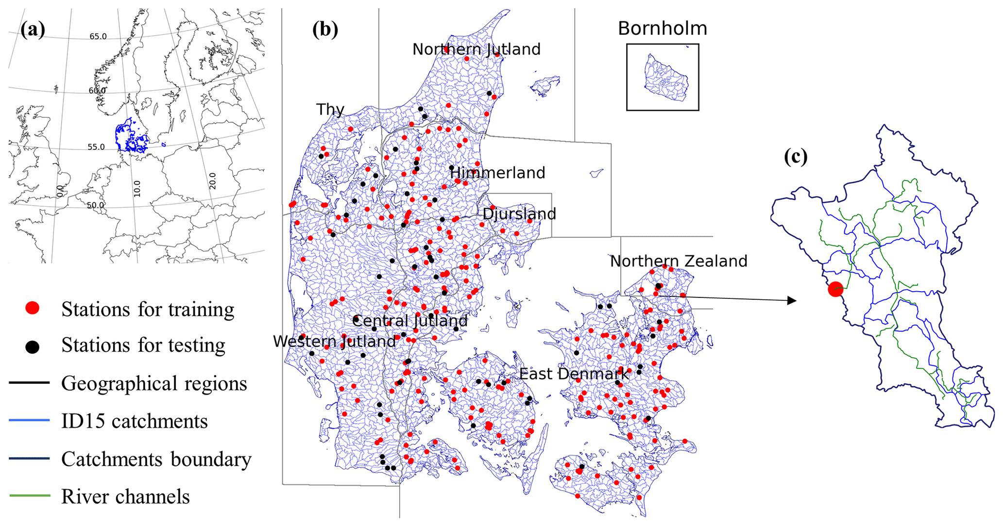
Figure 1Study area. (a) Geographic location of Denmark. (b) Subregions; ID15 catchments; and the locations of gauging stations, which have been randomly divided into training (254 stations) and testing groups (64 stations) for LSTM model development. (c) An outline of a gauged ID15 catchment (ID no. 32211117) located in northern Zealand.
2.1 Dataset
2.1.1 ID15 catchments
For various water management tasks, all of Denmark is subdivided into so-called ID15 catchments (Fig. 1). Each ID15 catchment represents a topographic basin with an average area of about 15 km2, and the total number of ID15 catchments is 3351. Out of these, 521 catchments lack a representation of the stream network in the DKM (mostly because they are small catchments draining directly to the sea) or are located on small islands and have been excluded in this study. With the selected 2830 ID15 catchments, we cover 90.60 % of the land area of Denmark. Figure 1b shows different scales of ID15 catchments, and each of the shapefiles represents a catchment unit, has data on flow direction, and connects with the upstream routing area, allowing us to obtain the total aggregated upstream area for all basins; see an example in Fig. 1c. The catchment boundary to any required points on river networks is defined by the identity index of the catchment unit. The ID15 catchments have been adjusted to connect with DKM discharge points (Q points), which are the grid points of the MIKE HYDRO River setup where simulated discharge time series are available (DHI, 2020), and hydrological stations.
Based on the ID15 catchment dataset, we prepared a dataset of catchment attributes and hydrometeorological time series for the 2830 catchments, like the widely used CAMELS series dataset (Addor et al., 2017; Alvarez-Garreton et al., 2018; Chagas et al., 2020; Coxon et al., 2020; Fowler et al., 2021; Höge et al., 2023). The dataset includes static catchment attributes, dynamic variables of climate forcings, streamflow observations, and DKM simulations. Climate forcings include precipitation, temperature, and potential ET. DKM-simulated streamflow for each ID15 catchment was extracted from the Q points at the catchment outlets. The other simulations are grid-based spatiotemporally distributed variables originating from DKM at 500 m resolution, including actual evapotranspiration, average soil water content, and phreatic depth. They were all spatially aggregated into a time series for each ID15 catchment, including the entire upstream area.
2.1.2 Climate forcings and basin attributes
The climate data used in this study include precipitation, mean temperature, and potential ET, which were obtained from the Danish Meteorological Institute (Scharling, 1999a, b). The temporal resolution of the climate data is daily, and the spatial resolution of precipitation is 10 and 20 km for both temperature and potential ET. Precipitation was corrected based on daily wind speed and temperature to correct for precipitation sensor undercatch (Stisen et al., 2011). The climate forcings are used as inputs for both the DKM and LSTM model.
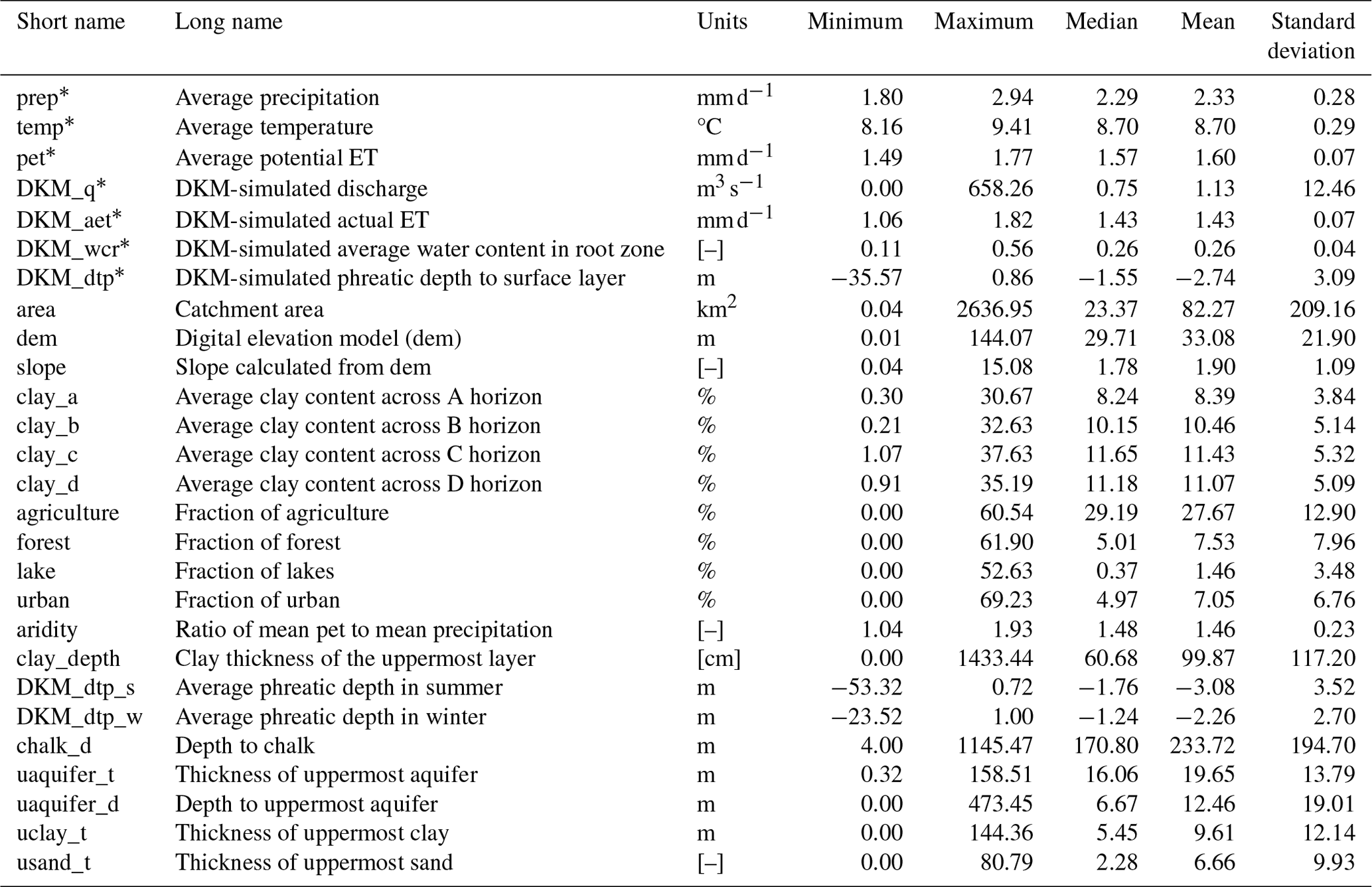
Catchment attributes, such as land use, soil type, topography, geology, and climate, play a pivotal role in hydrological modeling, as variations contribute significantly to the hydrological processes taking place in the basin. We selected 27 static catchments attributes which we consider impact the hydrological processes in Denmark (Table 1). The spatial distribution of these attributes is shown in Appendix A. The average elevation of all the catchments ranges from 0.01 to 144.07 m, with a median elevation of 29.71 m. The median slope is 1.78 % of all the catchments. The average clay content is higher in east than in west Jutland. The static catchment attributes include simulation outputs from the DKM: discharge, actual ET, water content in the root zone, and phreatic depth (Schneider et al., 2022b; Koch et al., 2021). The spatial distribution of phreatic depth shows it is low in north and middle Jutland. The median value of phreatic depth is −1.76 m in summer and high in winter, with a median value of −1.24 m. Agriculture is the main land use type occupying 28 % on average. Southern and central Jutland have higher chalk aquifer depth and clay thickness above the chalk aquifer.
Table 1Static catchment attributes.
∗ These variables include both catchment attributes and daily time series.
2.2 Benchmark models
2.2.1 Danish National Water Resources Model (DKM)
The DKM has been developed at the Geological Survey of Denmark and Greenland (GEUS) over the course of several decades (Henriksen et al., 2021, 2003; Højberg et al., 2013; Soltani et al., 2021; Stisen et al., 2020). It is built on the MIKE SHE hydrological modeling framework using a transient, fully distributed, physics-based description of the terrestrial hydrological cycle (Højberg et al., 2013; Stisen et al., 2020; Abbott et al., 1986; DHI, 2020); 3D subsurface flow is coupled with processes in the unsaturated zone, 2D overland flow, and surface water routing in streams. The model is run with daily climate forcings (Sect. 2.2.2) and is calibrated against daily streamflow observations from ∼300 stations across Denmark (stations shown in Fig. 1c) as well as groundwater head observations. It currently exists at two horizontal resolutions, 100 and 500 m. For our case, we use the 500 m version due to its reduced computational demand and the limited effect of enhanced grid resolution on streamflow simulations. For simulation of streamflow, MIKE SHE is coupled with the surface water model code MIKE HYDRO River. In the case of the DKM, simple streamflow routing is applied as the focus is on streamflow simulation (DHI, 2020). The MIKE SHE and MIKE HYDRO River models are coupled through river links, where water is exchanged between the river channel and land surface and subsurface. In the 500 m version of the DKM, approximately 20 000 km of water courses is represented in this manner.
2.2.2 LSTM rainfall–runoff model (LSTM-rr)
LSTM is a type of recurrent neural network (RNN) specifically developed to address the shortcomings of traditional RNNs when confronted with sequences featuring long-term dependencies (Hochreiter and Schmidhuber, 1997; Sutskever et al., 2014; Rahmani et al., 2020; Gers et al., 2000; Greff et al., 2017; Kratzert et al., 2018). These networks possess the remarkable ability to selectively retain or discard information over extended sequences. They achieve this using specialized memory cells that store and update information as it traverses the networks (Gers et al., 2000). LSTM networks are equipped with multiple hidden neurons and incorporate essential information-processing instants, namely the input, forget, and output gates. These gates play the main roles in regulating the flow of sequential information, enabling the network to determine what information should be preserved and what should be discarded at each time step. While a comprehensive understanding of LSTM networks can be found in numerous studies, readers with a background in hydrology are encouraged to explore the works of Kratzert et al. (2018) for more detailed insights.
LSTM-rr uses meteorological inputs, including precipitation, temperature, and potential ET, as dynamic variables, alongside catchment attributes as embedded static inputs, with the discharge observed at basin outlets as the target variable (De La Fuente et al., 2023; Hashemi et al., 2022; Koch and Schneider, 2022; Kratzert et al., 2021b, 2018). The networks are usually trained and tested using historical data from a group of gauged basins and applied to extrapolate streamflow for unmonitored periods or ungauged basins. LSTM-rr has gained popularity due to its ability to capture complex temporal dependencies and nonlinear relationships, and the predicted streamflow has often been found to outperform traditional hydrological models (Hauswirth et al., 2021; Frame et al., 2022; Lees et al., 2021; Wilbrand et al., 2023; Feng et al., 2020).
2.3 LSTM hybrid schemes
We created four LSTM models distinguished by input sequences and target variables as candidate hybrid models for streamflow simulations on a national scale (see Fig. 2). The tested models include (1) pre-training fine-tuning rainfall–runoff model, (2) dynamic input model with DKM simulations and climate forcing, (3) residual error prediction model, and (4) error factor prediction model. The first serves as a benchmark to assess the accuracy that can be obtained by a standalone LSTM model without a hybrid scheme. The remaining four models represent different implementations of hybrid models. The following subsections describe the details of these models.

Figure 2Input data, target variables, and abbreviated names of different LSTM hybrid models.
2.3.1 Pre-training and fine-tuning the LSTM rainfall–runoff model (LSTM-pf)
Pre-training and fine-tuning are techniques used to improve the performance of neural networks on specific tasks (MacNeil and Eliasmith, 2011; Käding et al., 2017; Cai and Peng, 2021). These techniques are commonly employed in transfer learning, where knowledge learned from one task or dataset is transferred to another related task or dataset (Li and Zhang, 2021; Tan et al., 2018). Pre-training involves training a neural network on a large dataset or a related task before fine-tuning it for the target task. This helps the model learn useful features and representations from the large dataset and grasp general patterns of the data. Fine-tuning means that a pre-trained neural network is taken and further trained on a smaller dataset specific to the target task, updating its weights accordingly. In this study, we pre-trained an LSTM-rr model based on all ID15 catchments, climate forcings as dynamic inputs, basin attributes as static inputs, and DKM-simulated streamflow as the target variable. This process enables the LSTM model to learn major features between climate data and the simulated discharge. Fine-tuning is then conducted on basins of observed discharge; i.e., the target variable is changed from DKM-simulated discharge to observations. The hyperparameters are the same for both pre-training and fine-tuning. The total number of epochs is equivalent to that of LSTM-rr, with the first half being allocated for pre-training and the second half dedicated to fine-tuning.
2.3.2 Hybrid dynamic inputs to the LSTM model (LSTM-q)
In this configuration, the dynamic inputs are expanded with DKM simulations that impact river streamflow, including the depth of the phreatic surface, average soil water content, actual ET, and DKM-simulated streamflow itself. The depth to phreatic surface varies among basins with different hydrogeological properties, like permeability of the subsurface materials, aquifers, and confining layers. Groundwater pumping for irrigation, industrial use, or drinking water supply can significantly alter the interaction between phreatic surface depth and river discharge. Pumping can lead to a lower groundwater table, reducing the groundwater contribution to river flow. DKM includes water extraction for drinking water supply and irrigation; thus, the variation in phreatic depth reflects the impacts of climate conditions and human activities.
2.3.3 LSTM residual error model (LSTM-qr)
Often, the streamflow of a river exhibits strong seasonality due to changes in precipitation and temperature throughout the year. Simulated streamflow and their associated errors often exhibit systematic patterns, such as overestimating baseflow or underestimating high flow during specific periods and rates. This occurs because of the limitations in model structures and parameters. The misfitting follows certain regular patterns that can potentially be identified through data-driven algorithms. Some studies attempted to predict the residuals between PBM-simulated streamflow and observations (Cho and Kim, 2022; Konapala et al., 2020). They argue that the variabilities in residuals are lower in comparison to the variabilities in the streamflow itself, and their results showed that the streamflow simulations could be improved after applying the predicted residuals to PBM-simulated streamflow.
However, special attention should be paid to the residual time series because data-driven methods cannot effectively learn or predict them when residuals consistently manifest as random noise. To test the whiteness of residuals between DKM simulations and observations, we analyze the autocorrelation to ensure that the time series of residuals are not simply related to noise. Figure 3 illustrates an example of the residuals between simulated and observed streamflow on a daily scale at a station. The residuals were calculated by observed streamflow with the DKM simulations subtracted, so a positive residual indicates that the DKM simulations are lower than observations. It can be observed in Fig. 3a that the simulated streamflow is typically underestimated in winter (high-flow seasons) and overestimated in the warm seasons (low-flow seasons), which consistently occurred every year in the example. The autocorrelation figure reveals several spikes outside the 99 % bounds, indicating that the time series of residuals are not white noise and could potentially be predicted by LSTM networks.
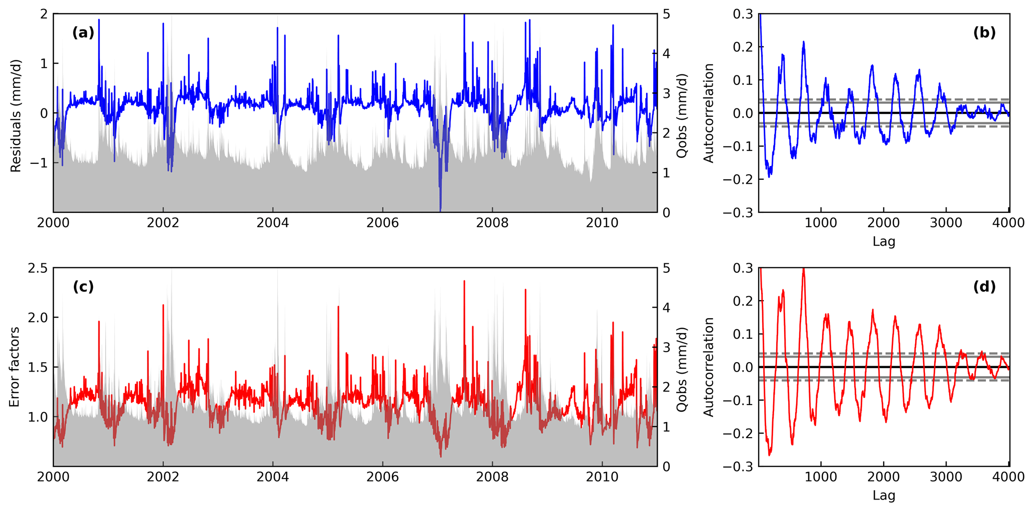
Figure 3Daily time series of streamflow residuals (a) and error factors (c) between DKM-simulated streamflow and observations at a hydrological station (ID no. 51350461); the grey area shows observed streamflow time series. Autocorrelation of the time series is displayed in (b) and (d) to test white noise of residuals and error factors. The horizontal grey lines in (b) and (d) correspond to 95 % (dash) and 99 % (solid) confidence bands.
2.3.4 LSTM error factor model (LSTM-qf)
The configurations of LSTM-qf are similar to those of LSTM-qr, but the target variables are relative error factors between observed streamflow and DKM simulations instead of absolute residuals. The error factors were calculated by dividing observations by DKM simulations, so a value of 1 means that DKM simulations are equal to observations. For example (Fig. 3), we can see that DKM underestimates the streamflow in winter and overestimates the streamflow in summer. Compared to streamflow residuals, error factors exhibit more variability and outliers (Fig. 3c). The results of the simulations are over 2 times lower than the observations during high-flow events, which could be due to a mismatch in the peak-flow dates. For instance, the error factors are extremely high on one date and drop to values of less than 1 on the following day, indicating a mismatch in the peak-flow times. The plot shows that the error factors in time series are correlated and can be predicted by data-driven algorithms.
2.4 Experiment settings
To assess the potential of various LSTM hybrid modeling schemes within both gauged and ungauged basins, we conducted a series of validation experiments. There are 318 gauged basins (Fig. 1), which were randomly partitioned into training basins consisting of 254 stations (80 %) and test basins comprising 64 stations (20 %). Streamflow was divided into a training period from 2000 to 2010, a testing period from 1990 to 1999, and a validation period from 2011 to 2019. The training and testing periods are the same as in DKM to ensure the comparability of LSTM models and DKM simulations. We followed the design by Koch and Schneider (2022) and created temporal split experiments and spatiotemporal split experiments to evaluate the performance of LSTM models in gauged and ungauged basins. The temporal split experiment used the 254 training stations for training during the period from 2000 to 2010, and the same stations were used for testing during the test period from 1990 to 1999. The spatiotemporal split-sample experiment uses 254 stations for training during 2000 to 2010, and the trained model was tested on 64 testing stations during 1990 to 1999.
The NeuralHydrology Python package is used to train and test all LSTM networks. The package is developed by Kratzert et al. (2022) and has been widely used in research after it was made open-source (Frame et al., 2021; Klotz et al., 2022; Koch and Schneider, 2022; Nearing et al., 2022; Wilbrand et al., 2023). All the LSTM hybrid schemes are trained with the NeuralHydrology package based on PyTorch on a server equipped with an NVIDIA A40 GPU (Paszke et al., 2019). The standard PyTorch implementation in the NeuralHydrology package, CudaLSTM, is used for LSTM training due to its efficiency. Dynamic inputs and static attributes are passed through embedding networks. The optimizer is Adam, and the loss function is the RMSE for all models.
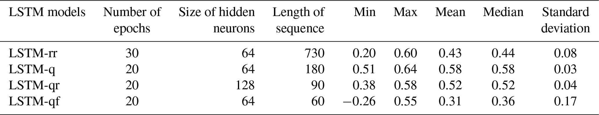
Before using LSTM networks for specific tasks, it is necessary to determine the values of critical hyperparameters. Since there is no standard method of finding an optimal set of hyperparameters for our case, we selected relevant hyperparameters based on previous studies and assessed their sensitivity (Cho and Kim, 2022; Hashemi et al., 2022; Kratzert et al., 2018). The selected hyperparameters include the number of training epochs, size of hidden neurons, and lookback length (LL) of the sequence. The other hyperparameters have fixed values, such as the dropout rate (0.4), batch size (128), and learning rate (10−3). The tested values for these hyperparameters are defined in Table 2. To assess the performance of all candidate hyperparameter combinations, a total of 96 () possible combinations were generated. The combination demonstrating the highest performance in terms of the mean Nash–Sutcliffe efficiency (NSE) values in the spatiotemporal split-sample experiment is chosen to configure the final LSTM models. Table 3 shows the optimal hyperparameters for LSTM models. LSTM-rr has a higher number of epochs and a greater sequence length compared to the hybrid scheme, and LSTM-qr has a greater size of hidden neurons. The standard deviation shows how dispersed the results are in relation to the mean, and LSTM-q has the lowest standard deviation, indicating that changes in hyperparameters have less effect on model performance.
Table 2The potential values of hyperparameters for LSTM models.

Table 3Optimal hyperparameters for LSTM models and the statistics of mean NSE in the spatiotemporal split experiment.
2.5 Model evaluations
The model performance is evaluated by the model NSE coefficient, which compares simulations to the average observations, quantifying the proportion of observed variance that the model can explain (Gupta and Kling, 2011). NSE ranges from negative infinity to 1, with 1 indicating a perfect match between model predictions and observations. We follow the model evaluation guidelines suggested by Moriasi et al. (2007) to determine if the model performance is very good (), good (), satisfactory (), or unsatisfactory (NSE≤0.5).
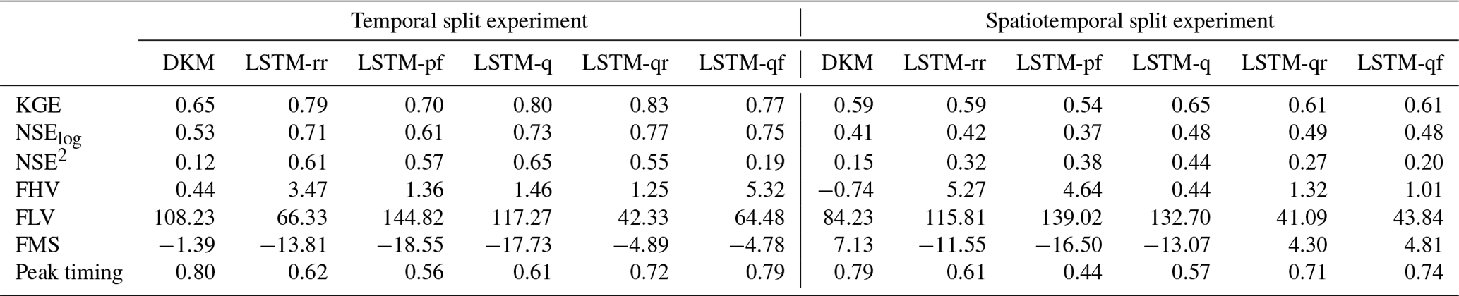
Additional metrics, including Kling–Gupta efficiency (KGE), logarithmic NSE (NSElog), squared NSE (NSE2), root mean square error (RMSE), high-segment volume (FHV), low-segment volume (FLV), mid-segment slope (FMS), and peak timing, are also calculated, and the results are presented in the Appendix. Details about these signature measures are explained in the literature (see, for example, Schneider et al., 2022a; Roy et al., 2023; Yilmaz et al., 2008; Gupta et al., 2009; and Kratzert et al., 2021a).
3.1 Long-term performance of LSTM hybrid schemes
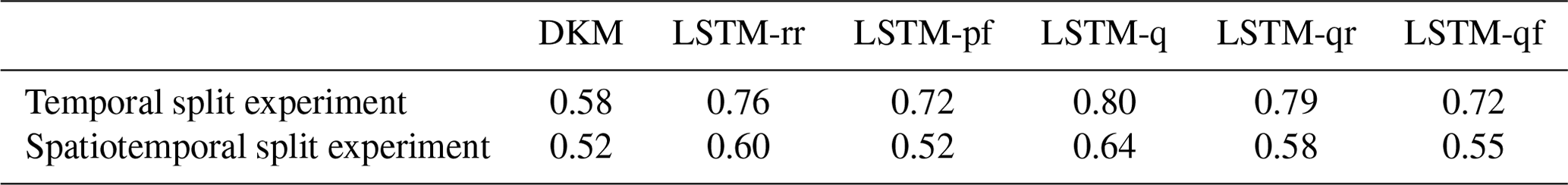
The cumulative distribution function (CDF) of NSE for the temporal split experiment and the spatiotemporal split experiment is shown in Fig. 4. Mean values of NSE of all the stations, which were used for ranking model performance, are listed in Table 4. In general, all LSTM models outperformed the DKM (Fig. 4a), underlining the potential of utilizing LSTM models for streamflow estimation. LSTM-q (mean NSE is 0.80) exhibits the best model performance, closely followed by LSTM-qr (mean NSE is 0.79), LSTM-rr (0.76), LSTM-pf (0.72), and LSTM-qf (mean NSE is 0.72) in the temporal split experiment. LSTM-qr has the highest KGE (0.83) and NSElog (0.77), indicating that the scheme is better for low-flow modeling. LSTM hybrid models show higher performance but did not alter the performance significantly compared with the benchmark model LSTM-rr.
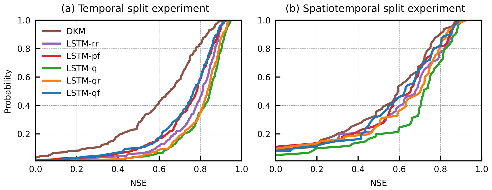
Table 4Mean NSE of DKM and the LSTM hybrid models in the temporal split experiment and the spatiotemporal split experiment.
The performance of all LSTM models decreased when applied to ungauged basins (Fig. 4b), as revealed by the spatiotemporal split experiment. LSTM-q outperforms LSTM-qr according to NSE in the spatiotemporal split experiments, indicating that LSTM-q is more effective for high-flow modeling. This is further supported by FHV, which measures the bias of peak flow where LSTM-q shows a lower error compared to LSTM-qr (see Appendix B1). In contrast, LSTM-qr demonstrates higher performance in low-flow conditions with lower FLV bias (41 %). The DKM exhibits a higher peak-timing error, while LSTM-rr and LSTM-q show the lower peak-timing error, and the other two hybrid models, i.e., LSTM-qr and LSTM-qf, rely on DKM-simulated discharge and also show a higher peak-timing error.
Figure 5 shows the spatial distribution of NSE of DKM at all stations and the enhancements in NSE achieved by LSTM hybrid modeling. DKM exhibits satisfactory performance (NSE>0.5) in 73 % of basins from the temporal split experiment and 64 % from the spatiotemporal split experiment. There are seven stations from the temporal split experiment and five stations from the spatiotemporal split experiment that have negative NSE values. DKM has difficulties in modeling the streamflow in basins covered by large lake areas, such as stations situated in Himmerland and northeast Zealand (Fig. 5a). LSTM hybrid models have improved the NSE at many stations, as illustrated in Fig. 5b–f. Stations in Himmerland, western Jutland, and eastern Denmark exhibit unsatisfactory performance of DKM (colored blue), while showing improved performance with LSTM models (colored red). Figure 5a shows the improvements of LSTM-rr compared to DKM. Many blue points in central Jutland, Himmerland, and Djursland can be seen, and such basins are located in areas with deeper groundwater levels (see Appendix A). Similar patterns are also shown in Fig. 5b, which displays the results of LSTM-pf. Figure 6d demonstrates that LSTM-q improved the performance of many stations in both temporal split and spatiotemporal split experiments, with fewer blue points compared to Fig. 5a and b. However, some stations that initially showed very good performance with DKM demonstrate degraded performance with LSTM models, indicating the difficulty in further improving streamflow estimation for already well-performing stations and maintaining their performance. Statistically, LSTM-rr improved discharge estimation at 89 % of stations in the temporal split experiment, while the improvement ratio is 56 % in the spatiotemporal split experiment. LSTM-q has improved NSE by 98 % and 74 % in spatial split/non-split experiments. The results of LSTM-qr are comparable to LSTM-q, while LSTM-qf shows limited improvement for ungauged basins, as seen by the numerous blue points in Fig. 5f. Although LSTM-q demonstrates the best overall performance, it still fails to enhance NSE at some stations, especially in the spatiotemporal split experiments.
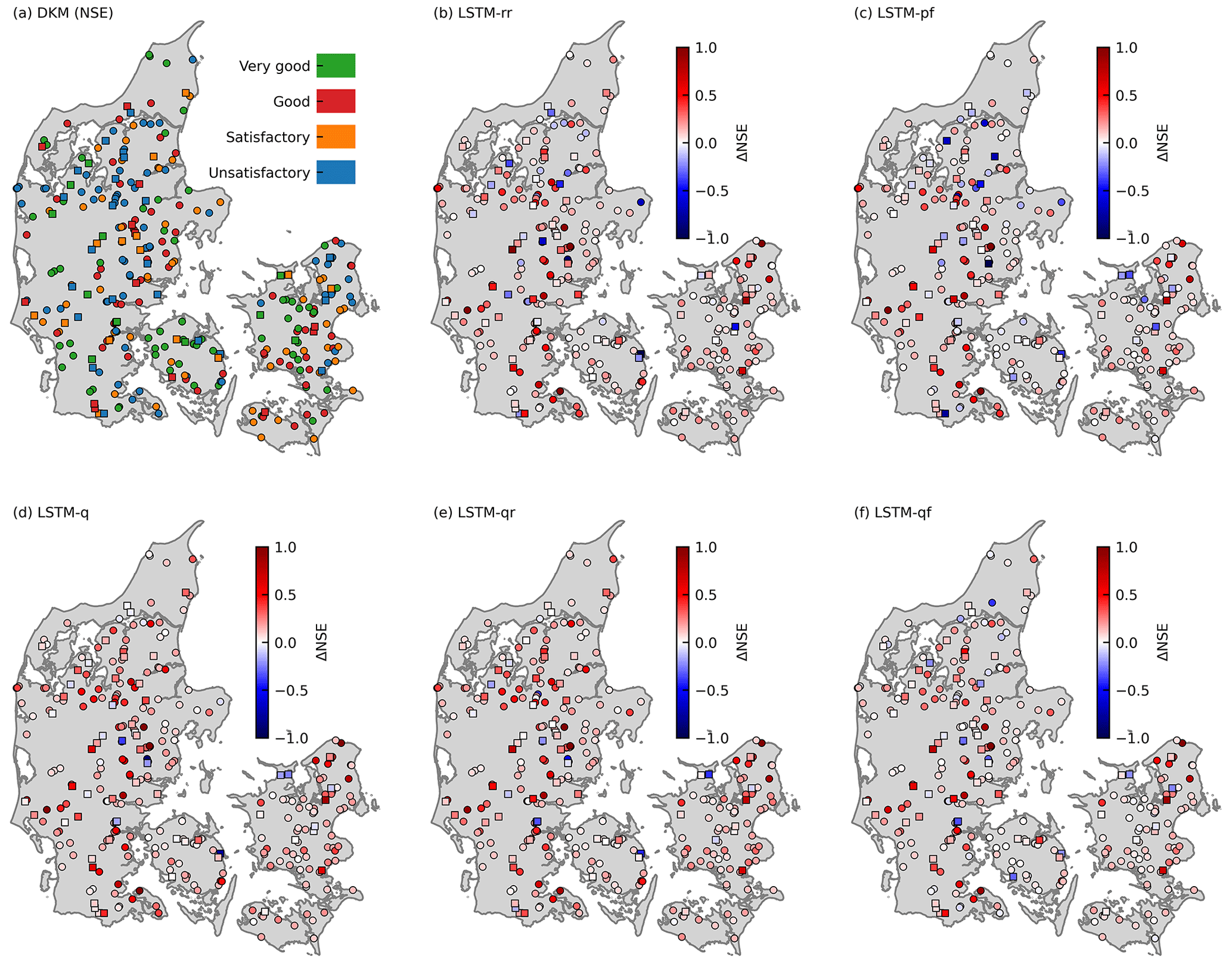
Figure 5Performance of DKM and LSTM model during the testing period (1990–1999) of the temporal split experiment (marked by circles) and the spatiotemporal split experiments (marked by squares). (a) The NSE of DKM. Panels (b)–(f) show the differences in NSE between DKM and LSTM ().
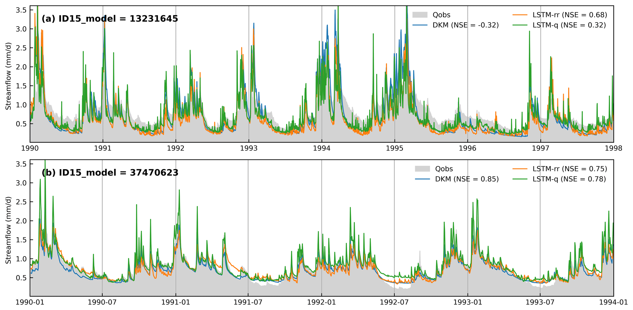
Figure 6Time series of the streamflow at two hydrological stations which were involved in the spatiotemporal split experiment.
Figure 6 presents the time series of the streamflow for two example stations from the spatiotemporal split experiment located in the western Jutland, which we have named basin A (ID no. 12430739; DKM has satisfactory results) and basin B (ID no. 37470623; DKM has very good results). DKM underestimates the low flow and overestimates the high flow in basin A, resulting in a negative NSE (). LSTM-rr and LSTM-q agree well with observations during high-flow seasons but tend to underestimate streamflow during low-flow periods. The simulated hydrograph of the LSTM hybrid models, though the performance is incomparable to LSTM-rr, improves the estimations during low-flow seasons. The hydrography shows that the simulated streamflow by models drops too early in low-flow seasons, while the observed discharge does not, which could be due to the influence of groundwater. However, the findings differ in basin B, where the DKM-simulated streamflow aligns well with observations but overestimates the discharge in some low-flow seasons and the NSE is 0.85. LSTM overestimated high flow, LSTM-rr underestimated it, and their performance is not as good as that of DKM. Basin B is spatially close to basin A, and the climate forcings are equivalent. We then compared the basin attributes of basins A and B with those of the basins used for LSTM training. The slope of basin B (5.03) is significantly higher than that of basin A (1.14) and most training basins (ranging from 0.258 to 4.580). The forest ratio of basin B is 27.61 %, whereas it is 5.98 % for basin A. These distinct differences between basin A and the training dataset result in the inferior performance of LSTM models. These results demonstrate the challenges of extrapolating streamflow to ungauged basins and the importance of selecting training datasets with diverse catchment attributes.
Figure 7 presents a heatmap of correlation coefficients between model performance (NSE and ΔNSE) of the different models and static basin attributes. Unsurprisingly, basin area positively correlates with all models' performance; i.e., performance generally is better for larger basins (Henriksen et al., 2021). DKM-simulated groundwater levels (dtp, dtp_s, and dtp_w) positively correlate with the NSE for all models, indicating that the models generally struggle to accurately simulate streamflow in basins with deeper groundwater levels (see the areas with groundwater levels lower than −5 m in Appendix A1). In Denmark, much of the streamflow is generated as baseflow and thus controlled by groundwater levels. With deeper groundwater levels, accurate representation of groundwater level dynamics becomes more challenging. The negative correlation between model performance and the share of lake area can be explained by the complex interactions in lake water balances, something both the DKM and the LSTM model struggle with. Similarly, increased urban share decreases model performance; again, this is likely due to complexities and heterogeneities in urban hydrology being inadequately represented in the models. Geological features such as the depth to the chalk, thickness of upper uppermost aquifer, and thickness of uppermost sand negatively correlate with the performance of both DKM and LSTM model. The reasons for this require further investigation. The changes in performance of the LSTM models compared to the DKM (ΔNSE) exhibit a negative correlation with basin area, suggesting that LSTM model improvements decrease with increasing basin size (Fig. 7b). This might be related to all basin information being aggregated across each basin for the LSTM models, whereas the distributed nature of the DKM allows for the representation of more complex streamflow generation processes (and routing) within basins. LSTM models show performance improvements for catchments with a higher share of lake areas. The representation of lake water balances and streamflow through lakes is one of the weaknesses of the DKM, which can be improved by LSTM.

Figure 7Correlations between the performance (NSE) and changes in performance () of different LSTM models and catchment static attributes. The black points indicate the correlations that pass the 95 % significance tests.
3.2 Event performance of LSTM hybrid schemes
The objective of developing different LSTM models is to identify an optimal hybrid scheme to support the operational modeling and forecasting framework, which the DKM is already a part of. A real-time module has been established to collect daily observations of climate forcings, including precipitation, temperature, and potential ET, which serve as inputs for a real-time DKM. Within the operational real-time framework, emphasis is placed on modeling extreme events. Therefore, in this section, we investigate the performance of LSTM hybrid schemes in modeling extremely high and low flows. Furthermore, based on the conclusions drawn from previous sections, LSTM-q outperforms the other hybrid models. We exclusively present the results of LSTM-q in this section. The hybrid model was retrained with additional data to obtain more accurate results. We set the training period to be from 1990 to 2010 and evaluated model performance on specific extreme events during the latest decade.
We selected four distinct wet periods (Fig. 8a–d) characterized by high peak flows across many regions of Denmark as well as two dry periods (Fig. 8e and f) marked by severe drought conditions. Figure 8 displays the observed streamflow and simulations from the DKM and LSTM-q averaged across all stations as well as the line chart of RMSE for all stations. LSTM-q (chosen based on its superior performance) shows improved RMSE compared to the DKM at most stations but fails at a few stations, as indicated by the tail of the fitted frequency density curve (Fig. 8a–d). The average RMSE decreased from 0.68 mm d−1 for DKM to 0.45 mm d−1 for LSTM-q for the flood events that occurred on 20 December 2011 (Fig. 8a). Similar improvements can also be observed for the rest of the flood events, with the RMSE decreasing from 0.73 to 0.52 mm d−1 (Fig. 8b), from 1.05 to 0.78 mm d−1 (Fig. 8c), and from 0.66 to 0.48 mm d−1 (Fig. 8d). Capturing peak flows accurately proves challenging for both DKM and the LSTM hybrid schemes, as the simulated streamflow values tend to be lower than those of observations during the four flooding events. The time of peak flow is consistently earlier in DKM compared to observations, as demonstrated in all selected events, which are improved by LSTM-q. The issue of miscapturing the peak time by the physically based DKM requires further investigation of precipitation time series. Two drought events that occurred in July 2018 and July 2019 exhibited a very low streamflow. LSTM-q demonstrates better performance compared with DKM, as depicted in Fig. 8e and f. The average RMSE decreased from 0.12 mm d−1 for DKM to 0.06 mm d−1 for LSTM-q during these events.
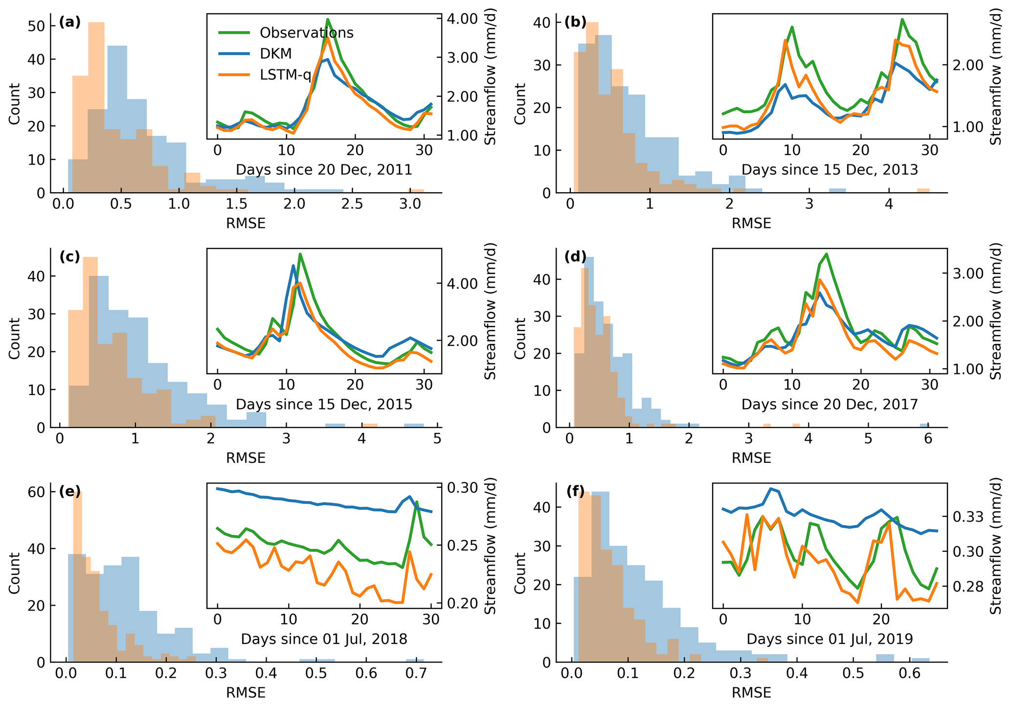
Figure 8Performance of DKM and LSTM-q during extreme events. (a–d) Four flooding events and (e, f) two drought events. In each subplot, the main figure shows the RMSE calculated across all stations and the fitted probability density function; an additional graph in the top right shows the averaged time series of the streamflow.
3.3 Comparison of LSTM models and DKM at a national level
After developing and identifying the optimal LSTM hybrid schemes, we extended their application from predicting streamflow in gauged basins to ungauged basins, such as the outlets of all ID15 catchments across Denmark. Figure 9 illustrates the high/median/low flow of DKM in all ID15 catchments from 2010 to 2020 and the residuals between LSTM-q and DKM in all ID15 catchments. Streamflow is high in western and central Jutland (Fig. 9a–c), which is consistent with the spatial distribution of precipitation (Appendix A1). DKM and LSTM model generally agree well with each other in most basins, with percentage differences close to 0. This further underlines the robustness of the LSTM models, in spatial extrapolation as well, as they manage to follow the simulated streamflow patterns from the DKM which is based on a spatially consistent setup, jointly calibrated for all of Denmark. However, discrepancies arise in certain basins, as indicated by deep-red and deep-blue colors in Fig. 9d–f, particularly during high- and low-flow conditions. In Jutland, the LSTM models tend to simulate higher low flows compared to DKM, while in eastern Denmark, the opposite pattern is observable (Fig. 9d). In western Jutland, where precipitation is higher and the DKM-simulated streamflow is larger than in other regions, the LSTM models predict lower high flows (Fig. 9e). The spatial patterns here are inconsistent with the averaged time series in Fig. 8, where DKM underestimated high flow in gauged basins (Fig. 8a–d) and overestimated low-flow events compared to LSTM-q (Fig. 8e and f).

Figure 9A comparison of simulated streamflow differences between DKM and LSTM model (LSTM-q). The first row depicts DKM-simulated streamflow during low-flow, high-flow, and mean-flow conditions; the second row shows the differences between DKM simulations and the LSTM-q predictions. The percent difference in the figure is defined as the difference between the LSTM model and DKM, calculated as percent diff = .
In this study, a series of experiments was conducted to enhance the performance of streamflow estimation on a national scale in Denmark. The main objective was to assess various configurations of LSTM models to identify the optimal configuration to serve as a hybrid model for streamflow prediction. The results revealed that utilizing LSTM models, especially the hybrid schemes that were coupled with physically based simulations, exhibited superior performance for both long-term periods (spanning a decade) and short-term extreme events (30 d); see results in Sect. 3.1 and 3.2.
Overall, we found that the trained LSTM models were robust, and their performance was relatively consistent across the tested hyperparameters. Figure 10 underlines that the variations in the NSE across the sensitivity analysis of 96 hyperparameter combinations are small. Previous studies often applied default hyperparameters for LSTM development, a practice that remains justifiable due to the generally limited impact of hyperparameter adjustments. However, it is necessary to mention that the robustness of LSTM models can be further enhanced through the incorporation of physical knowledge into the selection of hyperparameters. For instance, the selection of a lookback length for sequential time series data traditionally adheres to 365 d for LSTM rainfall–runoff models, a choice made to account for the seasonal dynamics in hydrological processes. Nevertheless, the lookback length can be reduced to under 3 months in the hybrid modeling schemes, as model performance remains reliably consistent across these diverse temporal scales. This suggests that in this case, the longer-term hydrological information is contained in the PBM outputs such as groundwater levels. Conversely, we find that the LSTM-rr model, without the DKM as input, benefits from a prolonged lookback length.

Figure 10The relationship between NSE and sequential lookback length (LL) of the spatiotemporal split experiment.
The design of the applied temporal split experiment and the spatiotemporal split experiment aimed at illustrating the potential performance of LSTM models in gauged and ungauged basins. In this study, the performance of LSTM models (NSE>0.8) in gauged basins is comparable to previous studies (Cho and Kim, 2022; Lees et al., 2021; Konapala et al., 2020; Frame et al., 2021). The performance dropped for ungauged basins (spatiotemporal split experiment in Fig. 4) and aligned well with Koch and Schneider (2022). Few studies conducted a comparable spatiotemporal holdout experiment (Koch and Schneider, 2022); thus, special attention should be paid to validating the performance of LSTM models over ungauged basins. Kratzert et al. (2019b) applied a 12-fold cross-validation experiment over the contiguous United States and found a limited drop in performance for the predictions in ungauged basins. However, the applied 8.3 % spatial holdout may not pose the most challenging validation test. In our study, we applied a larger, 20 % spatial holdout, and a more systematic k-fold validation test was hampered by the inconsistent length of observations across the Danish discharge stations.
The intricate interactions between groundwater and surface water have posed challenges for simulating streamflow using rainfall–runoff models in many basins in Denmark (Danapour et al., 2019; Duque et al., 2023). We tested LSTM-rr for streamflow estimation, and the results were encouraging, with the mean NSE improving from 0.58 (DKM) to 0.76 (Table 4). These improvements indicate the large potential of the LSTM-rr model for streamflow modeling. However, it is important to note that LSTM-rr may not perform well everywhere, as evidenced by its limitations in strongly groundwater-dependent regions, such as northern Jutland. LSTM-rr simulates quick responses to the variations in precipitation well but can fail to predict reduced baseflows due to depleted groundwater storage (Fig. 6a). Also, the performance drop between temporal and spatiotemporal holdout is most pronounced for LSTM-rr (NSE is reduced from 0.76 to 0.59). Therefore, it is important to emphasize the advantages of integrating physical data into the LSTM framework, and the adoption of hybrid schemes, such as LSTM-q and LSTM-qr, yielded improvements in the estimation of streamflow. These results align with the findings of previous studies (Feng et al., 2022; Frame et al., 2021; Hunt et al., 2022; Zhang et al., 2023; Cho and Kim, 2022; Konapala et al., 2020; Tang et al., 2023) that assessed the potential of hybrid modeling.
We tested four different hybrid systems: LSTM-pf, LSTM-q, LSTM-qr, and LSTM-qf. They all exhibited improved performance for streamflow estimation according to the evaluation metrics (mean NSE calculated in spatiotemporal split experiment), with the order of priority (from high to low) being . The better performance of LSTM-q is consistent with previous studies; for instance, Cho and Kim (2022) proved that WRF-Hydro-LSTM has a lower-percent bias than LSTM-rr. Tang et al. (2023), Frame et al. (2021), and Hunt et al. (2022) showed that LSTM models with additional datasets of hydrological signals as inputs as well as simulations of global hydrological models outperformed LSTM-rr. Our results further confirmed that LSTM models can be further enhanced by providing information from hydrological models.
There is an interesting point claiming that LSTM-qr is slightly better than LSTM-q according to KGE (Appendix B1). Konapala et al. (2020) pointed out that the LSTM-qr model was inferior to LSTM-q across the conterminous US, which is in line with our study. In their work, LSTM-qr showed comparable performance with LSTM-q when the NSE of PBM was larger than 0.75, and the improvement of LSTM-qr then decreased as the NSE of PBM decreased. Thus, the performance of LSTM-qr was overly constrained by the performance of the underlying PBM, whereas LSTM-q was found to be more flexible. In our study, DKM performs better than the PBM in Konapala et al. (2020) and 27 % of the stations have an NSE higher than 0.75, whereas the percentage is 18 % in their study. Thus, this can explain the slightly increased performance of LSTM-qr in our case, because the underlying PBM, the DKM, performs generally very well. Cho and Kim (2022) used a well-calibrated model, WRF-Hydro (NSE=0.72 and R=0.88), to predict residuals, and they share our conclusion that the residual model performs better. Therefore, a well-established PBM is important for the performance of hybrid schemes. The performance of LSTM-pf is not comparable to the other LSTM hybrid schemes, which differs from the conclusion of Koch and Schneider (2022). This can be explained by the fact that in the pre-training, the model is pre-trained on DKM-simulated streamflow from all 2830 ID15 catchments as the target variable, whereas the fine-tuning is performed on only the observation station data. This may introduce more complexity and noise for LSTM to learn. Koch and Schneider (2022) only pre-trained using simulated DKM-based streamflow at the same basin where observations were available. We also implemented an experiment that pre-trained a model on gauged basins only with DKM-simulated streamflow as target variables, fine-tuned the model with observations, and made the performance comparable to that of LSTM-rr. To our knowledge, LSTM-qf is a novel hybrid modeling scheme, tested for the first time in the present study. The performance of LSTM-qf is lower than LSTM-qr. This is likely related to the use of DKM-simulated streamflow as the denominator when calculating the error factors, which can be problematic if simulated streamflow is close to zero, resulting in large and instable factors. Figure 3 shows that the variability in error factors is larger, with more outliers than residual time series. Thereby, we recommend focusing on the residual approach instead of the factor approach in future work.
We intended to train a skillful LSTM model to be used to forecast discharge across Denmark in an operational real-time framework currently under development. However, the LSTM networks presented in this study were trained using a limited number of gauged basins, potentially failing to encompass the full spectrum of hydrological regimes, which decreased their capacity to capture certain features effectively. The catchments have a large variety of static attributes spatially, and the hydrological regimes change significantly across Denmark. While the hybrid schemes offer enhanced information and mitigate the issue of limited input data, such as LSTM-q and LSTM-qr, they fall short in distinguishing stations requiring further improvement or those already meeting requirements from the physical model. Consequently, this deficiency may explain why LSTM models exhibit inferior performance at fewer stations when compared to DKM. Enhancing the neural networks with a multi-representation approach, with data assimilation, or by developing specific DL models for different regions distinguished by regime information could be alternative solutions in the future (Hashemi et al., 2022; Feng et al., 2020).
Spatially, we predicted the streamflow at a large number of catchments, namely 2830 outlets, covering most of Denmark. The comparison between LSTM and PBM performance across the entire region gives some insights into the effect of controlling factors on the different models' performance, potentially guiding further model improvement (especially of the PBM). Another question that arises in this case of nested catchments is how LSTM models can be developed that produce consistent streamflow simulations along river courses, with as many Q points as there are distributed hydrological models. This is particularly useful, as many PBMs currently provide streamflow simulations at explicit grids or points within the catchment (Harrigan et al., 2023). Correcting the streamflow at each PBM simulation point offers advantages, such as improving the prediction of the extent of local flooding, assessing drought hazards, and estimating nitrate transport, all of which require a refined resolution of streamflow at local scales. This is why LSTM-qr and LSTM-qf hybrid schemes, which can be predicted at the basin outlets and, potentially, can be applied to all Q points within a subbasin, were considered in this study. Ideally, discharge routing in the river channel involves linear accumulation from upstream to downstream, and, therefore, we can use relative residuals or error factors not only at basin outlets but also for upstream locations. However, implementing such an idea is challenging, given that river-routing processes do not change linearly from up the stream to down the stream due to additional water from small tributaries, groundwater contributions, and river regulation. Further information on river routing and the relationship of streamflow between upstream Q points and outlets should be considered, and advanced methods should be investigated for distributing residuals and error factors to all the Q points upstream. On the other hand, the development of advanced DL methods, such as distributed LSTM schemes (Yu et al., 2024), or graph neural networks could be the solutions to this topic in the future (Sun et al., 2022).
This study aimed at identifying optimal LSTM hybrid schemes based on the Danish National Water Resources Model (DKM) to enhance streamflow estimation on a national scale. To achieve this, we developed different LSTM hybrid models with varying dynamic inputs and target variables and evaluated them under different scenarios, including temporal and spatiotemporal split experiments. The optimal LSTM model, i.e., LSTM-q, was further assessed for its performance in extreme events. Lastly, we compared the disparities between DKM and the optimal LSTM models, seeking insights into hydrological modeling from both perspectives. The key conclusions of this study are as follows:
-
LSTM models excel at modeling streamflow in Denmark, demonstrating superior performance compared to DKM. The LSTM-rr model performs satisfactorily in numerous basins, with a mean NSE of 0.76 in the temporal split experiment and 0.60 in the spatiotemporal split experiment. However, it faces challenges in simulating streamflow in groundwater-dominant regions as well as spatial transferability, which can be mitigated by employing hybrid LSTM models.
-
The best-performing hybrid model is LSTM-q, achieving mean NSE values of 0.80 in temporal split experiments. Also, in ungauged basins, hybrid schemes surpass the DKM performance, with a mean NSE of 0.64, compared to that of 0.52 of the DKM. In the spatiotemporal split experiment, LSTM-qr improved the accuracy compared to the DKM for 73 % of stations, while LSTM-q improved 67 %. Basin attributes such as catchment area, average clay content, and phreatic depth correlate positively with model performance, whereas factors like slope, DEM, lake ratio, urban ratio, and thickness of uppermost aquifers correlate negatively with model performance.
-
LSTM hybrid models also contribute to improving the modeling of extreme events. LSTM-qr and LSTM-q effectively reduce errors in DKM-simulated values during high- and low-flow periods in Denmark. But still, more efforts should be made to improve the modeling accuracy toward extreme values in the hydrographs, as LSTM models underestimate the peak flow of flooding events. Future considerations may include employing alternative objective functions like NSE2 or manually augmenting the occurrence of peak flow during model training.
The utilization of LSTM in river streamflow modeling heralds a promising perspective for hydrological predictions. Previous studies focused more on gauged basins, while this study contributes to the topic with a national-scale analysis. We found that the conventional LSTM-rr model has limited performance in regions with complex hydrological processes. Information from physical hydrological models is helpful, as indicated by the benefits across several hybrid schemes. Our future plans include evaluating the hybrid schemes in a real-time forecasting framework forced by forecasted climate data and developing distributed LSTM hybrid schemes.
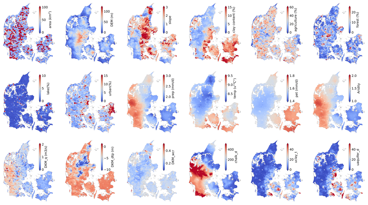
Figure A1Distribution of some catchment attributes.
B1 Additional model performance metrics
Table B1Additional metrics demonstrating model performance in both the temporal split experiment and the spatiotemporal split experiment.
B2 Overall model performance
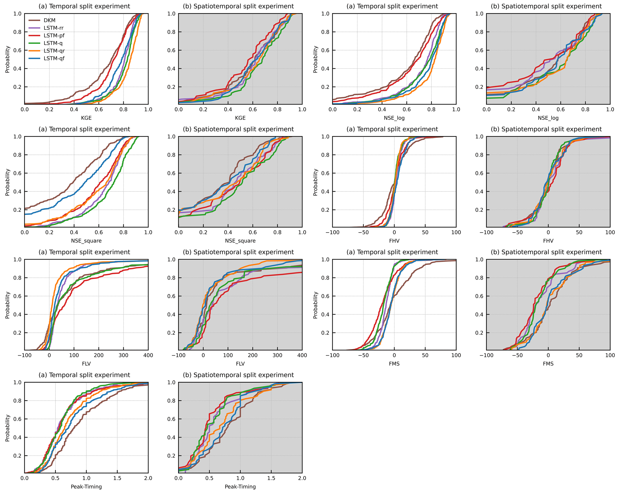
Figure B1Performance of benchmark models and LSTM hybrid models in the temporal split experiment (subplots with a white background) and the spatiotemporal split experiment (subplots with a grey background).
The LSTM code used in this study is based on the NeuralHydrology Python package, which can be accessed via https://neuralhydrology.github.io (Neural Hydrology, 2024). Upon request, the corresponding author will provide scripts for data pre-processing, post-processing, and visualization. The climate forcings and DKM simulations, as well as the in situ observations used in this study, are available upon request prior to the publication of the data paper.
All authors contributed to develop the original idea and design experiments. JL conducted the experiments in close cooperation with RJMS and JK and received further inputs from SS and LT. The code for data pre-processing, LSTM training and testing, data post-processing, and visualization were prepared by JL with support by RJMS and JK. JL and RJMS prepared the paper with contributions from JK, SS, and LT. All authors were involved in writing the paper.
The contact author has declared that none of the authors has any competing interests.
Publisher's note: Copernicus Publications remains neutral with regard to jurisdictional claims made in the text, published maps, institutional affiliations, or any other geographical representation in this paper. While Copernicus Publications makes every effort to include appropriate place names, the final responsibility lies with the authors.
The work presented in this paper was performed to enhance flood warnings for Denmark as part of the establishment of the Danish flood warning system (varslingssystem for oversvømmelser) from 2023 to 2026. The project is being led by the Danish Meteorological Institute (DMI) in cooperation with the Geological Survey of Denmark and Greenland (GEUS), the Danish Agency for Data Supply and Infrastructure (SDFI), the Danish Environmental Protection Agency (MST), the Danish Coastal Authority (KDI), and the Danish Environmental Portal (DMP). Special thanks are due to Hans Thodsen and Anker Lajer Højberg for providing the shapefile of the ID15 catchments and to Mark F. T. Hansen for verifying the connection between the ID15 catchments and DKM.
This paper was edited by Albrecht Weerts and reviewed by three anonymous referees.
Abbott, M. B., Bathurst, J. C., Cunge, J. A., O'Connell, P. E., and Rasmussen, J.: An introduction to the European Hydrological System – Systeme Hydrologique Europeen, “SHE”, 1: History and philosophy of a physically-based, distributed modelling system, J. Hydrol., 87, 45–59, https://doi.org/10.1016/0022-1694(86)90114-9, 1986.
Addor, N., Newman, A. J., Mizukami, N., and Clark, M. P.: The CAMELS data set: catchment attributes and meteorology for large-sample studies, Hydrol. Earth Syst. Sci., 21, 5293–5313, https://doi.org/10.5194/hess-21-5293-2017, 2017.
Alvarez-Garreton, C., Mendoza, P. A., Boisier, J. P., Addor, N., Galleguillos, M., Zambrano-Bigiarini, M., Lara, A., Puelma, C., Cortes, G., Garreaud, R., McPhee, J., and Ayala, A.: The CAMELS-CL dataset: catchment attributes and meteorology for large sample studies – Chile dataset, Hydrol. Earth Syst. Sci., 22, 5817–5846, https://doi.org/10.5194/hess-22-5817-2018, 2018.
Amendola, M., Arcucci, R., Mottet, L., Casas, C. Q., Fan, S., Pain, C., Linden, P., and Guo, Y.-K.: Data Assimilation in the Latent Space of a Neural Network, arXiv [preprint], https://doi.org/10.48550/arXiv.2012.12056, 2020.
Arsenault, R., Martel, J.-L., Brunet, F., Brissette, F., and Mai, J.: Continuous streamflow prediction in ungauged basins: long short-term memory neural networks clearly outperform traditional hydrological models, Hydrol. Earth Syst. Sci., 27, 139–157, https://doi.org/10.5194/hess-27-139-2023, 2023.
Baroni, G., Schalge, B., Rakovec, O., Kumar, R., Schüler, L., Samaniego, L., Simmer, C., and Attinger, S.: A Comprehensive Distributed Hydrological Modeling Intercomparison to Support Process Representation and Data Collection Strategies, Water Resour. Res., 55, 990–1010, https://doi.org/10.1029/2018WR023941, 2019.
Beven, K.: How to make advances in hydrological modelling, Hydrol. Adv. Theory Pract., 1969, 19–32, https://doi.org/10.2166/nh.2019.134, 2020.
Beven, K. J.: A discussion of distributed hydrological modelling, in: Distributed hydrological modelling, Springer, 255–278, https://doi.org/10.1007/978-94-009-0257-2_13, 1996.
Cai, Z. and Peng, C.: A study on training fine-tuning of convolutional neural networks, in: 2021 13th International Conference on Knowledge and Smart Technology (KST), 21–24 January 2021, Bangsaen, Chonburi, Thailand, 84–89, https://doi.org/10.1109/KST51265.2021.9415793, 2021.
Chagas, V. B. P., Chaffe, P. L. B., Addor, N., Fan, F. M., Fleischmann, A. S., Paiva, R. C. D., and Siqueira, V. A.: CAMELS-BR: hydrometeorological time series and landscape attributes for 897 catchments in Brazil, Earth Syst. Sci. Data, 12, 2075–2096, https://doi.org/10.5194/essd-12-2075-2020, 2020.
Cheng, M., Fang, F., Kinouchi, T., Navon, I. M., and Pain, C. C.: Long lead-time daily and monthly streamflow forecasting using machine learning methods, J. Hydrol., 590, 125376, https://doi.org/10.1016/j.jhydrol.2020.125376, 2020.
Cho, K. and Kim, Y.: Improving streamflow prediction in the WRF-Hydro model with LSTM networks, J. Hydrol., 605, 127297, https://doi.org/10.1016/j.jhydrol.2021.127297, 2022.
Coxon, G., Addor, N., Bloomfield, J. P., Freer, J., Fry, M., Hannaford, J., Howden, N. J. K., Lane, R., Lewis, M., Robinson, E. L., Wagener, T., and Woods, R.: CAMELS-GB: hydrometeorological time series and landscape attributes for 671 catchments in Great Britain, Earth Syst. Sci. Data, 12, 2459–2483, https://doi.org/10.5194/essd-12-2459-2020, 2020.
Curceac, S., Atkinson, P. M., Milne, A., Wu, L., and Harris, P.: Adjusting for Conditional Bias in Process Model Simulations of Hydrological Extremes: An Experiment Using the North Wyke Farm Platform, Front. Artif. Intell., 3, 1–16, https://doi.org/10.3389/frai.2020.565859, 2020.
Danapour, M., Højberg, A. L., Jensen, K. H., and Stisen, S.: Assessment of regional inter-basin groundwater flow using both simple and highly parameterized optimization schemes, Hydrogeol. J., 27, 1929–1947, https://doi.org/10.1007/s10040-019-01984-3, 2019.
De la Fuente, L. A., Ehsani, M. R., Gupta, H. V., and Condon, L. E.: Towards Interpretable LSTM-based Modelling of Hydrological Systems, EGUsphere [preprint], https://doi.org/10.5194/egusphere-2023-666, 2023.
Dembélé, M., Hrachowitz, M., Savenije, H. H. G., Mariéthoz, G., and Schaefli, B.: Improving the Predictive Skill of a Distributed Hydrological Model by Calibration on Spatial Patterns With Multiple Satellite Data Sets, Water Resour. Res., 56, 1–26, https://doi.org/10.1029/2019WR026085, 2020.
Devia, G. K., Ganasri, B. P., and Dwarakish, G. S.: A Review on Hydrological Models, Aquat. Pr., 4, 1001–1007, https://doi.org/10.1016/j.aqpro.2015.02.126, 2015.
Devitt, L., Neal, J., Coxon, G., Savage, J., and Wagener, T.: Flood hazard potential reveals global floodplain settlement patterns, Nat. Commun., 14, 2801, https://doi.org/10.1038/s41467-023-38297-9, 2023.
DHI: MIKE SHE User Guide and Reference Manual, https://manuals.mikepoweredbydhi.help/latest/Water_Resources/MIKE_SHE_Print.pdf (last access: 1 November 2022), 2020.
Duque, C., Nilsson, B., and Engesgaard, P.: Groundwater–surface water interaction in Denmark, WIRes Water, 10, 1–23, https://doi.org/10.1002/wat2.1664, 2023.
Fatichi, S., Vivoni, E. R., Ogden, F. L., Ivanov, V. Y., Mirus, B., Gochis, D., Downer, C. W., Camporese, M., Davison, J. H., and Ebel, B.: An overview of current applications, challenges, and future trends in distributed process-based models in hydrology, J. Hydrol., 537, 45–60, 2016.
Feng, D., Fang, K., and Shen, C.: Enhancing Streamflow Forecast and Extracting Insights Using Long-Short Term Memory Networks With Data Integration at Continental Scales, Water Resour. Res., 56, 1–24, https://doi.org/10.1029/2019WR026793, 2020.
Feng, D., Liu, J., Lawson, K., and Shen, C.: Differentiable, Learnable, Regionalized Process-Based Models With Multiphysical Outputs can Approach State-Of-The-Art Hydrologic Prediction Accuracy, Water Resour. Res., 58, e2022WR032404, https://doi.org/10.1029/2022WR032404, 2022.
Fowler, K. J. A., Acharya, S. C., Addor, N., Chou, C., and Peel, M. C.: CAMELS-AUS: hydrometeorological time series and landscape attributes for 222 catchments in Australia, Earth Syst. Sci. Data, 13, 3847–3867, https://doi.org/10.5194/essd-13-3847-2021, 2021.
Frame, J. M., Kratzert, F., Raney, A., Rahman, M., Salas, F. R., and Nearing, G. S.: Post-Processing the National Water Model with Long Short-Term Memory Networks for Streamflow Predictions and Model Diagnostics, J. Am. Water Resour. As., 57, 885–905, https://doi.org/10.1111/1752-1688.12964, 2021.
Frame, J. M., Kratzert, F., Klotz, D., Gauch, M., Shalev, G., Gilon, O., Qualls, L. M., Gupta, H. V., and Nearing, G. S.: Deep learning rainfall–runoff predictions of extreme events, Hydrol. Earth Syst. Sci., 26, 3377–3392, https://doi.org/10.5194/hess-26-3377-2022, 2022.
Gers, F. A., Schmidhuber, J., and Cummins, F.: Learning to forget: Continual prediction with LSTM, Neural Comput., 12, 2451–2471, 2000.
Ghorbani, A. and Zou, J.: Data shapley: Equitable valuation of data for machine learning, in: 36th Int. Conf. Mach. Learn. ICML 2019, 10–15 June 2019, Long Beach Convention Center, Long Beach, USA, 4053–4065, ISBN 9781510886988, 2019.
Goldstein, A., Kapelner, A., Bleich, J., and Pitkin, E.: Peeking Inside the Black Box: Visualizing Statistical Learning With Plots of Individual Conditional Expectation, J. Comput. Graph. Stat., 24, 44–65, https://doi.org/10.1080/10618600.2014.907095, 2015.
Greff, K., Srivastava, R. K., Koutnik, J., Steunebrink, B. R., and Schmidhuber, J.: LSTM: A Search Space Odyssey, IEEE T. Neur. Net. Lear., 28, 2222–2232, https://doi.org/10.1109/TNNLS.2016.2582924, 2017.
Gupta, H. V. and Kling, H.: On typical range, sensitivity, and normalization of Mean Squared Error and Nash-Sutcliffe Efficiency type metrics, Water Resour. Res., 47, 2–4, https://doi.org/10.1029/2011WR010962, 2011.
Gupta, H. V, Kling, H., Yilmaz, K. K., and Martinez, G. F.: Decomposition of the mean squared error and NSE performance criteria: Implications for improving hydrological modelling, J. Hydrol., 377, 80–91, 2009.
Harrigan, S., Zsoter, E., Cloke, H., Salamon, P., and Prudhomme, C.: Daily ensemble river discharge reforecasts and real-time forecasts from the operational Global Flood Awareness System, Hydrol. Earth Syst. Sci., 27, 1–19, https://doi.org/10.5194/hess-27-1-2023, 2023.
Hashemi, R., Brigode, P., Garambois, P.-A., and Javelle, P.: How can we benefit from regime information to make more effective use of long short-term memory (LSTM) runoff models?, Hydrol. Earth Syst. Sci., 26, 5793–5816, https://doi.org/10.5194/hess-26-5793-2022, 2022.
Hauswirth, S. M., Bierkens, M. F. P., Beijk, V., and Wanders, N.: The potential of data driven approaches for quantifying hydrological extremes, Adv. Water Resour., 155, 104017, https://doi.org/10.1016/j.advwatres.2021.104017, 2021.
Henriksen, H. J., Troldborg, L., Nyegaard, P., Sonnenborg, T. O., Refsgaard, J. C., and Madsen, B.: Methodology for construction, calibration and validation of a national hydrological model for Denmark, J. Hydrol., 280, 52–71, https://doi.org/10.1016/S0022-1694(03)00186-0, 2003.
Henriksen, H. J., Kragh, S. J., Gotfredsen, J., Ondracek, M., van Til, M., Jakobsen, A., Schneider, R. J. M., Koch, J., Troldborg, L., Rasmussen, P., Pasten-Zapata, E., and Stisen, S.: Udvikling af landsdækkende modelberegninger af terrænnære hydrologiske forhold i 100 m grid ved anvendelse af DK-modellen: Dokumentationsrapport vedr. modelleverancer til Hydrologisk Informations- og Prognosesystem. Udarbejdet som en del af Den Fællesoffen, GEUS, https://doi.org/10.22008/gpub/38113, 2021.
Henriksen, H. J., Schneider, R., Koch, J., Ondracek, M., Troldborg, L., Seidenfaden, I. K., Kragh, S. J., Bøgh, E., and Stisen, S.: A New Digital Twin for Climate Change Adaptation, Water Management, and Disaster Risk Reduction (HIP Digital Twin), Water-Sui, 15, 25, https://doi.org/10.3390/w15010025, 2023.
Herrera, P. A., Marazuela, M. A., and Hofmann, T.: Parameter estimation and uncertainty analysis in hydrological modeling, WIRes Water, 9, 1–23, https://doi.org/10.1002/wat2.1569, 2022.
Hochreiter, S. and Schmidhuber, J.: Long Short-Term Memory, Neural Comput., 9, 1735–1780, https://doi.org/10.1162/neco.1997.9.8.1735, 1997.
Höge, M., Kauzlaric, M., Siber, R., Schönenberger, U., Horton, P., Schwanbeck, J., Floriancic, M. G., Viviroli, D., Wilhelm, S., Sikorska-Senoner, A. E., Addor, N., Brunner, M., Pool, S., Zappa, M., and Fenicia, F.: CAMELS-CH: hydro-meteorological time series and landscape attributes for 331 catchments in hydrologic Switzerland, Earth Syst. Sci. Data, 15, 5755–5784, https://doi.org/10.5194/essd-15-5755-2023, 2023.
Højberg, A. L., Troldborg, L., Nyegaard, P., Ondracek, M., and Stisen, S.: Handling and linking data and hydrological models – experiences from the Danish national water resources model (DK-model), Modelcare2010, 141–144, ISBN 9787562524175, 2009.
Højberg, A. L., Troldborg, L., Stisen, S., Christensen, B. B. S. S., and Henriksen, H. J.: Stakeholder driven update and improvement of a national water resources model, Environ. Modell. Softw., 40, 202–213, https://doi.org/10.1016/j.envsoft.2012.09.010, 2013.
Hoy, A. Q.: Protecting water resources calls for international efforts, Science, 356, 814–815, https://doi.org/10.1126/science.356.6340.814, 2017.
Hunt, K. M. R., Matthews, G. R., Pappenberger, F., and Prudhomme, C.: Using a long short-term memory (LSTM) neural network to boost river streamflow forecasts over the western United States, Hydrol. Earth Syst. Sci., 26, 5449–5472, https://doi.org/10.5194/hess-26-5449-2022, 2022.
Käding, C., Rodner, E., Freytag, A., and Denzler, J.: Fine-tuning deep neural networks in continuous learning scenarios, Lect. Notes Comput. Sc. (including Subser. Lect. Notes Artif. Intell. Lect. Notes Bioinformatics), 10118 LNCS, 588–605, https://doi.org/10.1007/978-3-319-54526-4_43, 2017.
Kawaguchi, K., Bengio, Y., and Kaelbling, L.: Generalization in Deep Learning, in: Mathmatical Aspects of Deep Learning, Cambridge University Press, 112–148, https://doi.org/10.1017/9781009025096.003, 2022.
Ke, G., Meng, Q., Finley, T., Wang, T., Chen, W., Ma, W., Ye, Q., and Liu, T. Y.: LightGBM: A highly efficient gradient boosting decision tree, Adv. Neur. In., 3147–3155, ISBN 9781510860964, 2017.
Klotz, D., Kratzert, F., Gauch, M., Keefe Sampson, A., Brandstetter, J., Klambauer, G., Hochreiter, S., and Nearing, G.: Uncertainty estimation with deep learning for rainfall–runoff modeling, Hydrol. Earth Syst. Sci., 26, 1673–1693, https://doi.org/10.5194/hess-26-1673-2022, 2022.
Koch, J. and Schneider, R.: Long short-term memory networks enhance rainfall-runoff modelling at the national scale of Denmark, GEUS Bull., 49, 1–7, https://doi.org/10.34194/geusb.v49.8292, 2022.
Koch, J., Cornelissen, T., Fang, Z., Bogena, H., Diekkrüger, B., Kollet, S., and Stisen, S.: Inter-comparison of three distributed hydrological models with respect to seasonal variability of soil moisture patterns at a small forested catchment, J. Hydrol., 533, 234–249, 2016.
Koch, J., Gotfredsen, J., Schneider, R., Troldborg, L., Stisen, S., and Henriksen, H. J.: High Resolution Water Table Modeling of the Shallow Groundwater Using a Knowledge-Guided Gradient Boosting Decision Tree Model, Front. Water, 3, 1–14, https://doi.org/10.3389/frwa.2021.701726, 2021.
Konapala, G., Kao, S. C., Painter, S. L., and Lu, D.: Machine learning assisted hybrid models can improve streamflow simulation in diverse catchments across the conterminous US, Environ. Res. Lett., 15, 104022, https://doi.org/10.1088/1748-9326/aba927, 2020.
Kratzert, F., Klotz, D., Brenner, C., Schulz, K., and Herrnegger, M.: Rainfall–runoff modelling using Long Short-Term Memory (LSTM) networks, Hydrol. Earth Syst. Sci., 22, 6005–6022, https://doi.org/10.5194/hess-22-6005-2018, 2018.
Kratzert, F., Herrnegger, M., Klotz, D., Hochreiter, S., and Klambauer, G.: NeuralHydrology – Interpreting LSTMs in Hydrology, Lect. Notes Comput. Sc. (including Subser. Lect. Notes Artif. Intell. Lect. Notes Bioinformatics), 11700 LNCS, 347–362, https://doi.org/10.1007/978-3-030-28954-6_19, 2019a.
Kratzert, F., Klotz, D., Herrnegger, M., Sampson, A. K., Hochreiter, S., and Nearing, G. S.: Toward Improved Predictions in Ungauged Basins: Exploiting the Power of Machine Learning, Water Resour. Res., 55, 11344–11354, https://doi.org/10.1029/2019WR026065, 2019b.
Kratzert, F., Gauch, M., Nearing, G., Hochreiter, S., and Klotz, D.: Niederschlags-Abfluss-Modellierung mit Long Short-Term Memory (LSTM), Österreichische Wasser- und Abfallwirtschaft, 73, 270–280, https://doi.org/10.1007/s00506-021-00767-z, 2021a.
Kratzert, F., Klotz, D., Hochreiter, S., and Nearing, G. S.: A note on leveraging synergy in multiple meteorological data sets with deep learning for rainfall–runoff modeling, Hydrol. Earth Syst. Sci., 25, 2685–2703, https://doi.org/10.5194/hess-25-2685-2021, 2021b.
Kratzert, F., Gauch, M., Nearing, G., and Klotz, D.: NeuralHydrology – A Python library for Deep Learning research in hydrology, J. Open Source Softw., 7, 4050, https://doi.org/10.21105/joss.04050, 2022.
Kumari, N., Srivastava, A., Sahoo, B., Raghuwanshi, N. S., and Bretreger, D.: Identification of Suitable Hydrological Models for Streamflow Assessment in the Kangsabati River Basin, India, by Using Different Model Selection Scores, Nat. Resour. Res., 30, 4187–4205, https://doi.org/10.1007/s11053-021-09919-0, 2021.
Lees, T., Buechel, M., Anderson, B., Slater, L., Reece, S., Coxon, G., and Dadson, S. J.: Benchmarking data-driven rainfall–runoff models in Great Britain: a comparison of long short-term memory (LSTM)-based models with four lumped conceptual models, Hydrol. Earth Syst. Sci., 25, 5517–5534, https://doi.org/10.5194/hess-25-5517-2021, 2021.
Li, D. and Zhang, H. R.: Improved Regularization and Robustness for Fine-tuning in Neural Networks, Adv. Neur. In., 33, 27249–27262, 2021.
Liu, S., Wang, J., Wang, H., and Wu, Y.: Post-processing of hydrological model simulations using the convolutional neural network and support vector regression, Hydrol. Res., 53, 605–621, https://doi.org/10.2166/nh.2022.004, 2022.
Ma, K., Feng, D., Lawson, K., Tsai, W., Liang, C., Huang, X., Sharma, A., and Shen, C.: Transferring Hydrologic Data Across Continents – Leveraging Data-Rich Regions to Improve Hydrologic Prediction in Data-Sparse Regions, Water Resour. Res., 57, e2020WR028600, https://doi.org/10.1029/2020WR028600, 2021.
MacNeil, D. and Eliasmith, C.: Fine-tuning and the stability of recurrent neural networks, PLoS One, 6, e22885, https://doi.org/10.1371/journal.pone.0022885, 2011.
Moges, E., Demissie, Y., Larsen, L., and Yassin, F.: Review: Sources of hydrological model uncertainties and advances in their analysis, Water-Sui, 13, 1–23, https://doi.org/10.3390/w13010028, 2021.
Moriasi, D. N., Arnold, J. G., Van Liew, M. W., Bingner, R. L., Harmel, R. D., and Veith, T. L.: Model evaluation guidelines for systematic quantification of accuracy in watershed simulations, T. ASABE, 50, 885–900, 2007.
Nearing, G. S., Klotz, D., Frame, J. M., Gauch, M., Gilon, O., Kratzert, F., Sampson, A. K., Shalev, G., and Nevo, S.: Technical note: Data assimilation and autoregression for using near-real-time streamflow observations in long short-term memory networks, Hydrol. Earth Syst. Sci., 26, 5493–5513, https://doi.org/10.5194/hess-26-5493-2022, 2022.
Neural Hydrology: Using Neural Networks in Hydrology, GitHub, https://neuralhydrology.github.io (last access: 20 March 2023), 2024.
Nevo, S., Morin, E., Gerzi Rosenthal, A., Metzger, A., Barshai, C., Weitzner, D., Voloshin, D., Kratzert, F., Elidan, G., Dror, G., Begelman, G., Nearing, G., Shalev, G., Noga, H., Shavitt, I., Yuklea, L., Royz, M., Giladi, N., Peled Levi, N., Reich, O., Gilon, O., Maor, R., Timnat, S., Shechter, T., Anisimov, V., Gigi, Y., Levin, Y., Moshe, Z., Ben-Haim, Z., Hassidim, A., and Matias, Y.: Flood forecasting with machine learning models in an operational framework, Hydrol. Earth Syst. Sci., 26, 4013–4032, https://doi.org/10.5194/hess-26-4013-2022, 2022.
Pakoksung, K. and Takagi, M.: Effect of DEM sources on distributed hydrological model to results of runoff and inundation area, Model. Earth Syst. Environ., 7, 1891–1905, https://doi.org/10.1007/s40808-020-00914-7, 2021.
Paszke, A., Gross, S., Massa, F., Lerer, A., Bradbury, J., Chanan, G., Killeen, T., Lin, Z., Gimelshein, N., Antiga, L., Desmaison, A., Kopf, A., Yang, E., DeVito, Z., Raison, M., Tejani, A., Chilamkurthy, S., Steiner, B., Fang, L., Bai, J., and Chintala, S.: PyTorch: An Imperative Style, High-Performance Deep Learning Library, Adv. Neural Info. Proc. Syst., 32, ISBN 9781713807933, 2019.
Rahmani, F., Lawson, K., Ouyang, W., Appling, A., Oliver, S., and Shen, C.: Exploring the exceptional performance of a deep learning stream temperature model and the value of streamflow data, Environ. Res. Lett., 16, 024025, https://doi.org/10.1088/1748-9326/abd501, 2020.
Refsgaard, J. C., Stisen, S., and Koch, J.: Hydrological process knowledge in catchment modelling – Lessons and perspectives from 60 years development, Hydrol. Process., 36, 1–20, https://doi.org/10.1002/hyp.14463, 2022.
Roy, A., Kasiviswanathan, K. S., Patidar, S., Adeloye, A. J., Soundharajan, B. S., and Ojha, C. S. P.: A Novel Physics-Aware Machine Learning-Based Dynamic Error Correction Model for Improving Streamflow Forecast Accuracy, Water Resour. Res., 59, e2022WR033318, https://doi.org/10.1029/2022WR033318, 2023.
Sahraei, S., Asadzadeh, M., and Unduche, F.: Signature-based multi-modelling and multi-objective calibration of hydrologic models: Application in flood forecasting for Canadian Prairies, J. Hydrol., 588, 125095, https://doi.org/10.1016/j.jhydrol.2020.125095, 2020.
Satoh, Y., Yoshimura, K., Pokhrel, Y., Kim, H., Shiogama, H., Yokohata, T., Hanasaki, N., Wada, Y., Burek, P., Byers, E., Schmied, H. M., Gerten, D., Ostberg, S., Gosling, S. N., Boulange, J. E. S., and Oki, T.: The timing of unprecedented hydrological drought under climate change, Nat. Commun., 13, 3287, https://doi.org/10.1038/s41467-022-30729-2, 2022.
Scharling, M.: Klimagrid Danmark – Nedbør, lufttemperatur og potentiel fordampning 20×20 & 40×40 km – Metodebeskrivelse, Danish Meteorol. Inst., https://www.dmi.dk/fileadmin/user_upload/Rapporter/TR/1999/tr99-12.pdf (last access: 2 July 2024), 1999a.
Scharling, M.: Klimagrid Danmark Nedbør 10×10 km (ver. 2) – Metodebeskrivelse, Danish Meteorol. Inst., 15–17, https://www.dmi.dk/fileadmin/user_upload/Rapporter/TR/1999/tr99-15.pdf (last access: 2 July 2024), 1999b.
Schneider, R., Henriksen, H. J., and Stisen, S.: A robust objective function for calibration of groundwater models in light of deficiencies of model structure and observations, J. Hydrol., 613, 128339, https://doi.org/10.1016/j.jhydrol.2022.128339, 2022a.
Schneider, R., Koch, J., Troldborg, L., Henriksen, H. J., and Stisen, S.: Machine-learning-based downscaling of modelled climate change impacts on groundwater table depth, Hydrol. Earth Syst. Sci., 26, 5859–5877, https://doi.org/10.5194/hess-26-5859-2022, 2022b.
Shen, Y., Ruijsch, J., Lu, M., Sutanudjaja, E. H., and Karssenberg, D.: Random forests-based error-correction of streamflow from a large-scale hydrological model: Using model state variables to estimate error terms, Comput. Geosci., 159, 105019, https://doi.org/10.1016/j.cageo.2021.105019, 2022.
Silvestro, F., Gabellani, S., Rudari, R., Delogu, F., Laiolo, P., and Boni, G.: Uncertainty reduction and parameter estimation of a distributed hydrological model with ground and remote-sensing data, Hydrol. Earth Syst. Sci., 19, 1727–1751, https://doi.org/10.5194/hess-19-1727-2015, 2015.
Slater, L. J., Arnal, L., Boucher, M.-A., Chang, A. Y.-Y., Moulds, S., Murphy, C., Nearing, G., Shalev, G., Shen, C., Speight, L., Villarini, G., Wilby, R. L., Wood, A., and Zappa, M.: Hybrid forecasting: blending climate predictions with AI models, Hydrol. Earth Syst. Sci., 27, 1865–1889, https://doi.org/10.5194/hess-27-1865-2023, 2023.
Soltani, M., Bjerre, E., Koch, J., and Stisen, S.: Integrating remote sensing data in optimization of a national water resources model to improve the spatial pattern performance of evapotranspiration, J. Hydrol., 603, 127026, https://doi.org/10.1016/j.jhydrol.2021.127026, 2021.
Stisen, S., Sonnenborg, T. O., Højberg, A. L., Troldborg, L., and Refsgaard, J. C.: Evaluation of Climate Input Biases and Water Balance Issues Using a Coupled Surface-Subsurface Model, Vadose Zone J., 10, 37–53, https://doi.org/10.2136/vzj2010.0001, 2011.
Stisen, S., Ondracek, M., Troldborg, L., Schneider, R. J. M., and van Til, M. J.: National Vandressource Model. Modelopstilling og kalibrering af DK-model 2019, GEUS, Copenhagen, https://doi.org/10.22008/gpub/32631, 2020.
Sun, A. Y., Jiang, P., Yang, Z.-L., Xie, Y., and Chen, X.: A graph neural network (GNN) approach to basin-scale river network learning: the role of physics-based connectivity and data fusion, Hydrol. Earth Syst. Sci., 26, 5163–5184, https://doi.org/10.5194/hess-26-5163-2022, 2022.
Sutskever, I., Vinyals, O., and Le, Q. V.: Sequence to sequence learning with neural networks, Adv. Neur. In., 4, 3104–3112, 2014.
Tan, C., Sun, F., Kong, T., Zhang, W., Yang, C., and Liu, C.: A survey on deep transfer learning, Lect. Notes Comput. Sc. (including Subser. Lect. Notes Artif. Intell. Lect. Notes Bioinformatics), 11141 LNCS, 270–279, https://doi.org/10.1007/978-3-030-01424-7_27, 2018.
Tang, S., Sun, F., Liu, W., Wang, H., Feng, Y., and Li, Z.: Optimal Postprocessing Strategies With LSTM for Global Streamflow Prediction in Ungauged Basins, Water Resour. Res., 59, 1–16, https://doi.org/10.1029/2022WR034352, 2023.
Wang, Y., Liu, J., Li, C., Liu, Y., Xu, L., and Yu, F.: A data-driven approach for flood prediction using grid-based meteorological data, Hydrol. Process., 37, e14837, https://doi.org/10.1002/hyp.14837, 2023.
Wang, Y. H., Gupta, H. V., Zeng, X., and Niu, G. Y.: Exploring the Potential of Long Short-Term Memory Networks for Improving Understanding of Continental- and Regional-Scale Snowpack Dynamics, Water Resour. Res., 58, e2021WR031033, https://doi.org/10.1029/2021WR031033, 2022.
Wi, S. and Steinschneider, S.: On the need for physical constraints in deep learning rainfall–runoff projections under climate change: a sensitivity analysis to warming and shifts in potential evapotranspiration, Hydrol. Earth Syst. Sci., 28, 479–503, https://doi.org/10.5194/hess-28-479-2024, 2024.
Wilbrand, K., Taormina, R., ten Veldhuis, M., Visser, M., Hrachowitz, M., Nuttall, J., and Dahm, R.: Predicting streamflow with LSTM networks using global datasets, Front. Water, 5, 116612, https://doi.org/10.3389/frwa.2023.1166124, 2023.
Winsemius, H. C., Schaefli, B., Montanari, A., and Savenije, H. H. G.: On the calibration of hydrological models in ungauged basins: A framework for integrating hard and soft hydrological information, Water Resour. Res., 45, 1–15, https://doi.org/10.1029/2009WR007706, 2009.
Wu, H., Hu, T., Liu, Y., Zhou, H., Wang, J., and Long, M.: TimesNet: Temporal 2D-Variation Modeling for General Time Series Analysis, arXiv [preprint], https://doi.org/10.48550/arXiv.2210.02186, 2022.
Yilmaz, K. K., Gupta, H. V., and Wagener, T.: A process-based diagnostic approach to model evaluation: Application to the NWS distributed hydrologic model, Water Resour. Res., 44, 1–18, https://doi.org/10.1029/2007WR006716, 2008.
Yu, Q., Tolson, B. A., Shen, H., Han, M., Mai, J., and Lin, J.: Enhancing long short-term memory (LSTM)-based streamflow prediction with a spatially distributed approach, Hydrol. Earth Syst. Sci., 28, 2107–2122, https://doi.org/10.5194/hess-28-2107-2024, 2024.
Zhang, T., Liang, Z., Li, W., Wang, J., Hu, Y., and Li, B.: Statistical post-processing of precipitation forecasts using circulation classifications and spatiotemporal deep neural networks, Hydrol. Earth Syst. Sci., 27, 1945–1960, https://doi.org/10.5194/hess-27-1945-2023, 2023.
Zhang, Y., Ragettli, S., Molnar, P., Fink, O., and Peleg, N.: Generalization of an Encoder-Decoder LSTM model for flood prediction in ungauged catchments, J. Hydrol., 614, 128577, https://doi.org/10.1016/j.jhydrol.2022.128577, 2022.