Soil moisture modeling with ERA5-Land retrievals, topographic indices, and in situ measurements and its use for predicting ruts

Spatiotemporal modeling is an innovative way of predicting soil moisture and has promising applications that support sustainable forest operations. One such application is the prediction of rutting, since rutting can cause severe damage to forest soils and ecological functions.

In this work, we used ERA5-Land soil moisture retrievals and several topographic indices to model variations in the in situ soil water content by means of a random forest model. We then correlated the predicted soil moisture with rut depth from different trials.

Our spatiotemporal modeling approach successfully predicted soil moisture with Kendall's rank correlation coefficient of 0.62 (R² of 64 %). The final model included the spatial depth-to-water index, topographic wetness index, stream power index, as well as temporal components such as month and season, and ERA5-Land soil moisture retrievals. These retrievals were shown to be the most important predictor in the model, indicating a large temporal variation. The prediction of rut depth was also successful, resulting in Kendall's correlation coefficient of 0.61.

Our results demonstrate that by using data from several sources, we can accurately predict soil moisture and use this information to predict rut depth. This has practical applications in reducing the impact of heavy machinery on forest soils and avoiding wet areas during forest operations.

1 Introduction

For decades, forestry research has sought solutions to accurately predict the trafficability of forest soils (Mattila and Tokola, 2019; White et al., 2012; Murphy et al., 2007). In order to further sustainable forest management, efficient protection of forest soils is mandatory (Vega-Nieva et al., 2009; Picchio et al., 2020; Uusitalo et al., 2019). Heavy harvesting and forwarding machines have been frequently associated with severe soil damage, particularly when operating on soils with low bearing capacity (Horn et al., 2007; Allman et al., 2017). Soil compaction is a common consequence of harvesting operations (Ampoorter et al., 2010; Eliasson, 2005; DeArmond et al., 2021) and has been shown to be detrimental to a number of ecological functions, including soil biota (Beylich et al., 2010), hydrological patterns, and nutrient supply, with potential drawbacks on plant growth and site productivity (Curzon et al., 2022). In addition to soil compaction, machine traffic can also result in deep ruts (Horn et al., 2007; Ala-Ilomäki et al., 2021; Poltorak et al., 2018), which affect site hydrology and increase anaerobic conditions at the rut's base, where air-filled porosity is reduced, leading to minimized soil aeration (Hansson et al., 2019).

The risk of causing high degrees of soil compaction and rutting is mainly attributed to soil properties such as initial soil bulk density and texture, as well as the current soil water content (Cambi et al., 2015; Crawford et al., 2021). Moist soils show a higher susceptibility to damage since the internal friction is decreased through water embracing soil particles (Hillel, 1998), reducing the soil bearing capacity and the ability for elastic responses to machine-induced impacts (McNabb et al., 2001).

To support forestry management and machine operators, accurate cartographic information on soils with low bearing capacity is essential (Jones and Arp, 2017; Sirén et al., 2019; Campbell et al., 2013). However, existing models that rely on detailed soil maps to retrieve soil mechanical parameters (e.g., Grüll, 2011; Heubaum, 2015) require a high level of input data, and high-resolution soil maps are only available for selected areas, hindering their large-scale application (Vega-Nieva et al., 2009; Kristensen et al., 2019). Therefore, researchers have turned to topographic modeling as a more promising approach (Lidberg et al., 2020; White et al., 2012), as it requires only digital elevation models (DEMs), which are increasingly available for most parts of Europe (Hoffmann et al., 2022; Guo et al., 2017). One topographic index that has been extensively studied is the “depth-to-water” (DTW) concept, originally developed and tested at the University of New Brunswick by Meng, Ogilvie, and Arp, as described by Murphy et al. (2007, 2009). The DTW concept calculates flow lines across areas of interest by determining a flow accumulation and selecting lines that originate at a set threshold of accumulated upstream contributing areas. Using a cost function that considers the cell-to-cell slopes, the vertical distances from each cell within a raster to the nearest simulated flow line are ascertained. DTW is well documented (e.g., White et al., 2012; Vega-Nieva et al., 2009; Murphy et al., 2011).

Previous research has shown that the DTW index performs relatively well in predicting wet areas in forested formerly glaciated landscapes compared to other indices (Ågren et al., 2014; Larson et al., 2022). Recent studies have explored further developments in moisture prediction by utilizing machine learning algorithms applied to a variety of freely available data and diverse retrieved information, including different topographic indices calculated on DEMs. Ågren et al. (2021) used 28 topographic predictor variables in the XGBoost (eXtreme Gradient Boosting) model (Chen et al., 2021) to predict soil moisture across the entire Swedish forest landscape at high resolution (2 × 2 m). Although topographic modeling approaches are widely used, they often fail to adjust for seasonal changes in soil water regimes. Static maps may not adequately represent temporal occurrences of flow lines, wet fields, or water-saturated soils. Earlier, the DTW concept was designed to offer a potential solution by enabling the calculation of different scenarios ranging from “very dry” or “frozen” to “wet” soil conditions. However, selecting the most accurate DTW scenario requires high expertise (Leach et al., 2017: p. 5434; Lidberg et al., 2020), and mistakes can lead to reduced accuracy and result in potential soil damages that could be avoided.

Therefore, we believe that the next crucial step in soil moisture modeling is to incorporate a temporal component that enables the prediction of rasters for any given time and area. One approach to achieve this was designed by Schönauer et al. (2022), who developed a spatiotemporal prediction model. Dynamic satellite-based retrievals of soil moisture with coarse spatial resolution (Soil Moisture Active Passive mission) were combined with high-resolution but static topographic maps. This resulted in improved performance in predicting moisture values across time series conducted on sites in Finland, Germany, and Poland. The incorporation of a dynamic component into the prediction model enabled reflection of the current overall moisture conditions on the study sites. This allowed us to calculate daily prediction grids that could support forestry practice and enable the guidance of machine operators on sites to avoid traffic on wet areas susceptible to damages. However, a validation of predicting rut depth by models of this kind has not been facilitated yet.

The effectiveness of soil moisture modeling, whether based on static or dynamic independent variables, is ultimately constrained by the quality of the dependent variable, which in this case is in situ soil moisture. Manual measurements of soil moisture have been conducted in numerous studies using different devices, such as handheld time domain reflectometry sensors (Kemppinen et al., 2018; Uusitalo et al., 2019) or impedance measuring techniques (e.g., Schönauer et al., 2021b). Despite the potential inaccuracies associated with these techniques (Walker et al., 2004; Francesca et al., 2010), they offer significant advantages in terms of flexibility, scalability, low investment costs, and minimal maintenance. Another option is the use of continuously measuring sensor networks (e.g., Oliveira et al., 2021), which can provide relatively reliable measurements but with limited spatial coverage due to the high costs of installation and maintenance.

In this study, we built upon the approach developed by Schönauer et al. (2022) by incorporating additional data sources, including additional topographic indices, soil maps, and soil moisture retrievals from ERA5-Land for two soil depths. The study also used two types of data sources for soil moisture measurements: manual measurements using a handheld moisture meter and data from two continuously measuring sensor networks. We argue that manual measurements are simpler and can be applied to larger areas, while sensor networks are more expensive and limited to chosen locations.

The study had two main objectives: (1) to train soil moisture models using the two individual data sets (manual measurements and sensor networks) and evaluate their prediction performance and (2) to select the best combination of predictor variables (e.g., topographic indices and ERA5-Land values) using a repeated cross-validation approach and compare the best models with rut depth data obtained during four trials using a forwarder.

2 Material and methods

To model soil water content (SWC), random forest models were trained using two separate data sets: manual in situ measurements using an impedance measuring technique (IMT) and continuously measuring soil sensor networks (SSNs). To both data sets we added predictor variables derived from topographic indices (e.g., depth-to-water and topographic wetness index), soil maps, SWC estimates from the ERA5-Land campaign (SWC_ERA), and numerical values for date (month and season). We performed cross-validation and reduced features stepwise to choose the best-performing model. Subsequently, the two final models (for IMT and SSNs) were used to predict SWC for the positions and dates of different field trials with a forwarder. During these field trials, rut depth data were captured and compared to the predictions from the final SWC models (Fig. 1).

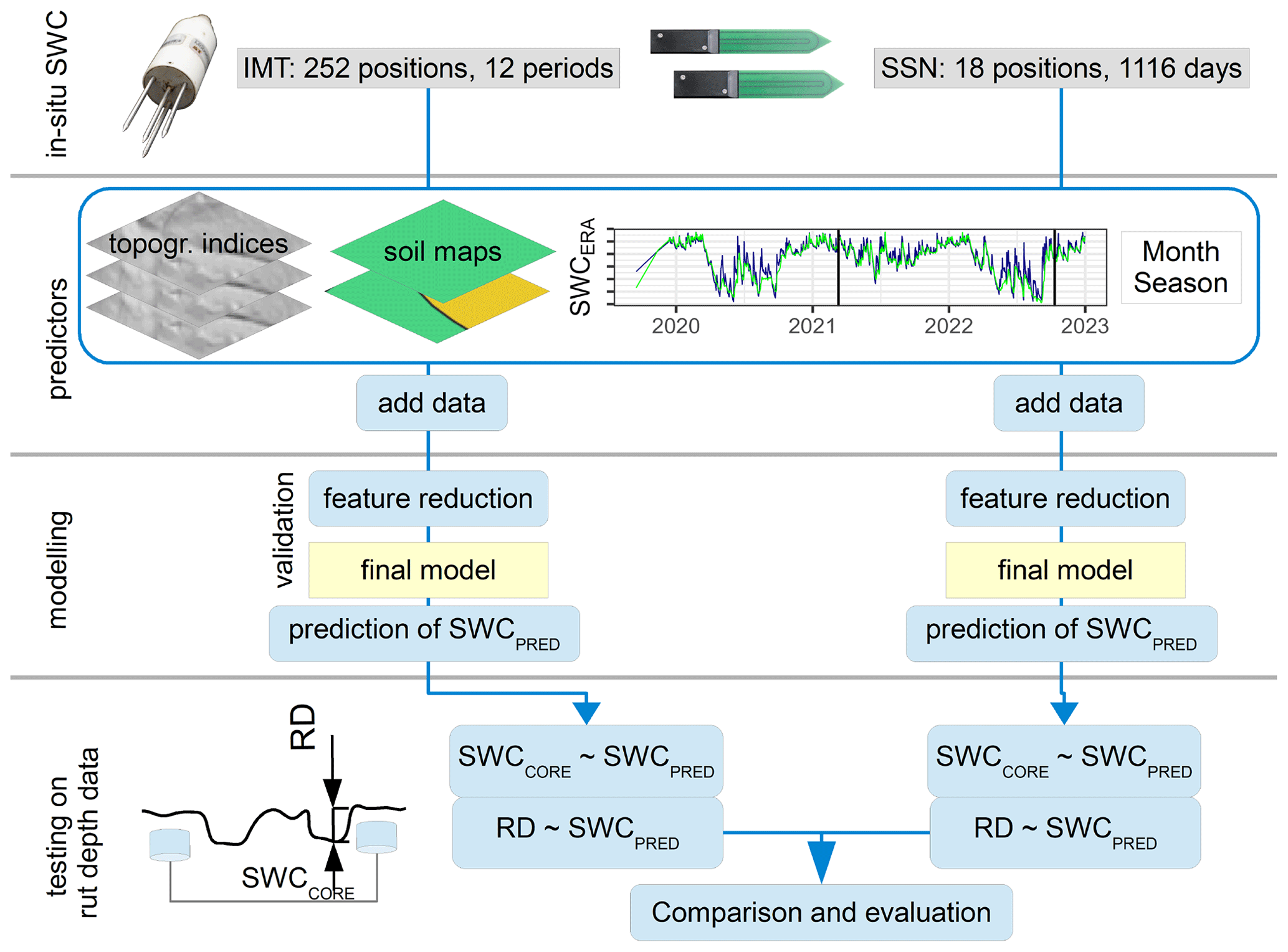
Figure 1 Soil water content (SWC; [%]) was predicted using models trained on two data sets: in situ measurements (IMT) and soil sensor networks (SSNs). Input variables included topographic indices, soil type data, SWC estimates from ERA5-Land (SWC_ERA), and date values. Through cross-validation, we selected the final models used to predict SWC_PRED for various positions and dates during trials with a forwarder. Model estimates were compared with in situ SWC_CORE and rut depth (RD; [cm]).

2.1 Study sites

The data acquisition of volumetric SWC [%] and the trials with a forwarder were conducted in two forest stands located near the city of Arnsberg in North Rhine-Westphalia, Germany (Fig. 2). The forest stands were situated at an altitude of approximately 250 m on common soil types such as Cambisol and Stagnosol on claystone and sandstone from the Devonian and the Carboniferous period (Table 1).

Table 1 Characteristics of the study sites where soil water content was captured and field trials with a forwarder were performed.

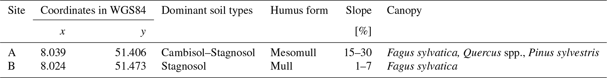
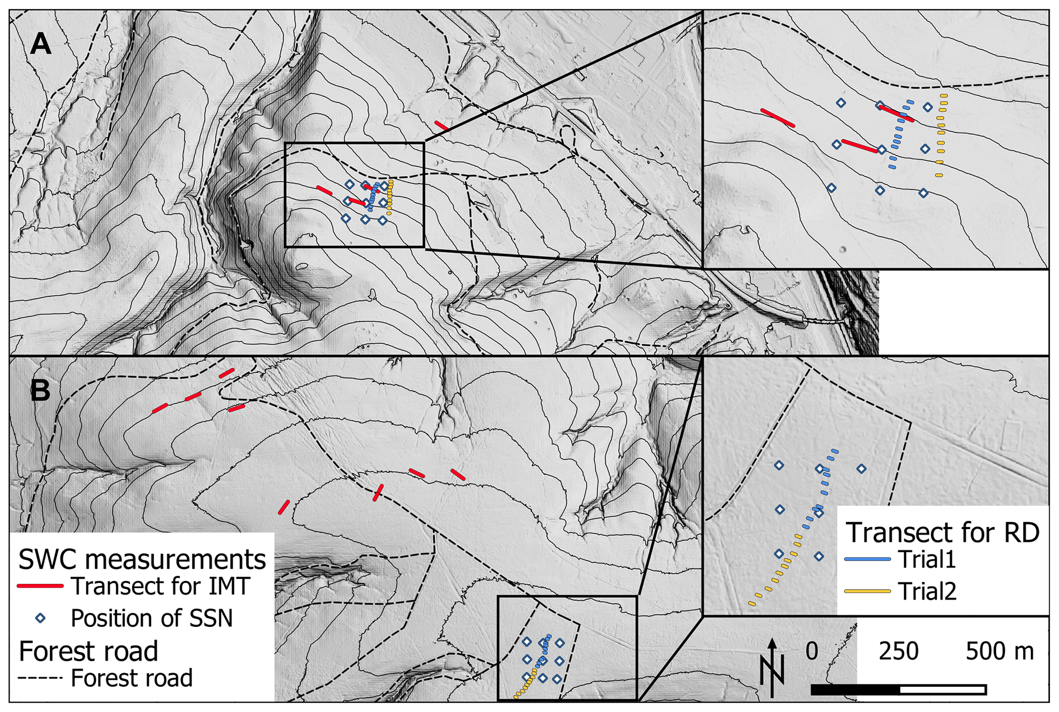
Figure 2 The map indicates the locations of two experimental areas on a hill-shaded digital elevation model with 10 m contour lines. Site A (A; coordinates x, y in WGS84 at 8.039, 51.406) and Site B (B; coordinates 8.024, 51.473) were used for collecting time series data on soil water content (SWC). SWC was measured using a handheld soil moisture meter (impedance measuring technique, IMT) along transects (red lines), each containing 21 measuring positions (2 m spacing). In addition, a soil sensor network (SSN) was used to continuously capture SWC at 18 positions (white rhombus). The map also indicates the locations of 40 transects (in crop-outs) used for measuring rut depth (RD) during relatively wet conditions (Trial_WET; blue lines) and drier conditions (Trial_DRY; orange lines).

2.2 Soil moisture models

2.2.1 In situ soil moisture

Two sets of in situ data of soil moisture were used: (1) manual measurements of SWC were performed using a HH2 Moisture Meter (Delta-T Devices Ltd, England), which applies an impedance measuring technique (i.e., IMT) (Eijkelkamp Agrisearch Equipment, 2013), and (2) data from a continuously measuring soil sensor network (i.e., SSN).

The IMT data used for this study were previously used for the validation by Schönauer et al. (2022) and consisted of 12 measuring transects. The transects were placed in various positions in broadleaved forests, known to be temporarily wet or sensitive for machine traffic, with each transect having a length of 40 m. SWC was measured with a spacing of 2 m along the transects. To measure SWC, measuring rods of 60 mm length were vertically inserted into the soil after removing the humus layer. The measurements were taken almost monthly between September 2019 and October 2020 (Fig. 3b). The IMT data consisted of 2184 observations. Overall, this data set offers a relatively high level of spatial granularity with 252 measuring positions. However, the temporal resolution of the data is relatively low with only monthly measuring campaigns conducted.

The SSN was launched in December 2019 and the data were obtained from continuously measuring SMT100 sensors (TRUEBNER GmbH, Germany), placed on two sites, each having nine positions with a spacing of 50 × 50 m. At each position, two sensors were placed at a depth of 10 cm in the mineral soil and with a temporal resolution of 15 min. The data from these sensors were averaged for each position and each of the 1116 d captured (data until 31 December 2022 were included), resulting in a total of 16 351 observations after omitting all missing values. While this data set provides a high level of temporal granularity, it suffers from a low level of spatial granularity due to the limited number of positions sampled.

To enable the incorporation of seasonal effects in the modeling approaches, we transformed the date of each measurement into numeric vectors, resulting in the variables of the month and season. The coding used for the seasons was as follows: 1 for March, April, and May; 2 for June, July, and August; 3 for September, October, and November; and 4 for December, January, and February.

To enable the creation of spatiotemporal data, the positions of all measuring locations were captured using post-processed signals from a GNSS (global navigation satellite system) device (Trimble R2 RTK rover, Trimble, Colorado, USA). These data were then fused with a range of topographic indices. To achieve this, values of several topographic indices were extracted at each measuring position of IMT and SSN.

2.2.2 Topographic indices

For calculating topographic indices, we used a freely available digital elevation model (DEM), as provided by the Bezirksregierung Köln (2020). The resolution of this model was 1 × 1 m with a vertical accuracy of ±0.2 m. Using the free programming language R (version 4.0.2; R Core Team, 2023) and RStudio (version 2022.07.2; Posit Software, PBC (formerly RStudio), Massachusetts, USA), along with the package “rgrass” (Bivand et al., 2023) to utilize GRASS GIS (Awaida and Westervelt, 2020) commands in the R interface, the command “r.hydrodem” was used to “remove all sinks” (flags −a) from the DEM. Thereafter, we calculated depth-to-water (DTW) maps. To generate these maps, we followed the script by Schönauer and Maack (2021) and used flow initiation areas (FIA) of the sizes 0.25 ha (DTW025), 1.00 ha (DTW1), and 4.00 ha (DTW4), which account for different overall soil moisture conditions. A smaller FIA results in a DTW map of wetter conditions as the network of simulated flow lines expands, while a larger FIA represents drier conditions. For further details, refer to Murphy et al. (2009, 2011).

The topographic wetness index (TWI) represents the tendency for water to accumulate at any point in the catchment (Quinn et al., 1991), while the stream power index (SPI) represents the power of water flow at any point in the catchment and the gravitational forces that move water downslope (Moore et al., 1991). To compute TWI, we used the “r.watershed” command in GRASS GIS, as conceived by Sørensen and Seibert (2007). TWI was calculated as ln($\mathit{\alpha }/\tan \left(\mathit{\beta }\right))$, where α is the cumulative upslope area draining through a point per unit contour length, and tan(β) is the local slope angle. SPI was calculated as α ⋅ tan(β) (Moore et al., 1991). Flow accumulation, representing the absolute amount of overland flow passing through each cell, was also included as a variable. TWI, SPI, and flow accumulation were calculated on an aggregated DEM with a spatial resolution of 15 × 15 m. This resolution has been shown to exhibit a stronger correlation with SWC, as observed in prior work where resolutions ranging from 1 to 20 m were tested (data not shown), and can be assumed to be more robust (Ågren et al., 2014). In addition, we calculated the variable slope [°] using the R package “raster” (Hijmans, 2020).

2.2.3 Soil maps

Soil maps of North Rhine-Westphalia were originally generated at a scale of 1:5000 from forest site surveys. We included soil type information (Soil05) for the analysis. While these maps are not available across the entire region of North Rhine-Westphalia, they were provided for the study sites by the Geological Survey of North Rhine-Westphalia. By contrast, soil maps with a scale of 1:50 000 are available for the entirety of North Rhine-Westphalia (Soil50).

2.2.4 Temporal soil water content from ERA5-Land

ERA5-Land is a global reanalysis data set providing hourly estimates of meteorological variables at a spatial resolution of 9 × 9 km, including soil moisture [m³ m⁻³] at the top soil layer (0–7 cm (“layer 1”, L1) and at a depth of 7–28 cm (“layer 2”, L2). ERA5-Land data are retrieved by assimilating satellite and atmospheric forcing (Muñoz-Sabater et al., 2021).

We opted for ERA5-Land retrievals to address the temporal component of SWC, as this data set offers a dependable representation of soil moisture values and their variations across global regions, rendering it suitable for various geophysical applications (Lal et al., 2022). Additionally, this decision is grounded on two key assumptions: (1) the spatial variability in the SWC is relatively low compared to its temporal variability. (2) The spatial extent of our measurement locations is small and cannot be adequately captured by satellite-based Earth observation data. Even Sentinel-1, a mission within the Copernicus Programme by the European Space Agency renowned for supporting high-resolution (1 × 1 km) surface soil moisture product generation (Peng et al., 2021), would have limited utility in providing spatial information for our study sites. For instance, the maximum distance between rut depth transects (Sect. 2.3.2) was 200 m. Furthermore, since Sentinel-1 focuses on surface soil moisture using the C band, we assume that ERA5-Land's soil moisture estimates for deeper layers might offer a better fit for our data, as suggested by similar findings presented by Fjeld et al. (2024).

We utilized the API provided by Climate Data Store (CDS) (Copernicus Climate Change Service, 2019) and the R package “ecmwfr” (Hufkens et al., 2019) to download daily grids (at 14:00 UTC) of layers 1 and 2. The downloaded data covered both the whole time span of our data and the two measuring sites. Both sites were situated in one 9 × 9 km raster cell of ERA5-Land. The land cover for this cell was derived from Bezirksregierung Köln (2023), showing that open land (e.g., grassland and crops) dominated with 52 % of the total cover, whereas forests occurred on approximately 31 % of the cell size, followed by 12 % coverage from infrastructure, 3 % loose material, and 2 % waterbodies.

After downloading the data, we stacked the daily grids and extracted the corresponding values at each measuring position, giving SWC_ERAL1 and SWC_ERAL2.

All data, the topographic information, soil types, numerical values of date and the dynamic variables from ERA5-Land were merged with in situ data, either IMT or SSN.

2.2.5 Modeling

The modeling approach described here was applied separately for both data sets of IMT and SSN (and for both data sets combined).

Initially, we fitted a linear model with SWC as the dependent variable and SWC_ERAL1, SWC_ERAL2, month, season, DTW025, DTW1, DTW2, DTW4, slope, TWI, SPI, accumulation, Soil05, and Soil50 as the independent variables. We then used this linear model to check the data for autocorrelations and subsequently eliminated variables with a variance inflation factor > 10 through an iterative process, reducing one variable at a time. Also, the feature selection according to the Boruta algorithm (package “Boruta”; Kursa and Rudnicki, 2010) was applied.

We then trained random forest models (Breiman, 2001), repeatedly reported as efficient in predicting complex data (Cavalli et al., 2023; Carranza et al., 2021; Kemppinen et al., 2018), using the “ranger” package (Wright and Ziegler, 2017) with a 10-fold cross-validation with five repetitions. For each of the 50 models in the validation of one configuration, we noted the mean of Kendall's coefficient of correlation τ (since different sample sizes occurred) of the random forests and the representative standard deviation. In addition, the least important variable according to impurity and its frequency within the 50 validation sets were traced. The variable noted most frequently as least important was then removed, and a new cross-validation was performed on SWC ∼ (n−1) variables, with n being the number of predictors in the model trained previously. This process was repeated until only one predictor variable remained.

To avoid temporal autocorrelations at the measuring positions, position IDs were used to select the folds of the cross-validations.

2.2.6 Selection of the final model

To select the final random forest model for each data partition, we examined the maximum τ values obtained and multiplied them by 0.99 (according to Hauglin et al., 2021). This was done to penalize the use of an unnecessarily high number of predictor variables. We selected the model with the least number of predictor variables within this 1 % range as the final model. The final models (built on IMT and SSN data) were then used to predict rasters of SWC_PRED, which were visually evaluated. Subsequently, the outputs of the final models were compared to rut depths and in situ SWC at the machine-operating trails.

2.3 Data from field trials with a forwarder

2.3.1 Rut depth (RD)

During the field trials conducted in two forest stands at two seasons, a fully loaded forwarder (John Deere 1210G, eight-wheel model, total mass of 28 Mg (18 Mg machine weight + 10 Mg loading)) was used. The first trial was conducted on section 1 of an existing machine-operating trail on 11 March 2021 during generally wet conditions (Trial_WET). The second trial was conducted on subsequent section 2 of the same machine trail on 11 October 2022 during drier conditions (Trial_DRY) (Fig. 2; Site B) or in close proximity of section 1 (Site A), as the machine trail there was not long enough for both sections.

The four trials were positioned near the sensors of the SSN (Fig. 2) and, in the case of Site A, near the IMT measuring transects. On Site B, the IMT transects were located at a distance of 530 to 1300 m. Moreover, there is a temporal lag between the IMT measuring campaigns and the field trials (Fig. 3). This discrepancy stems from the IMT data being collected as part of a separate research project.

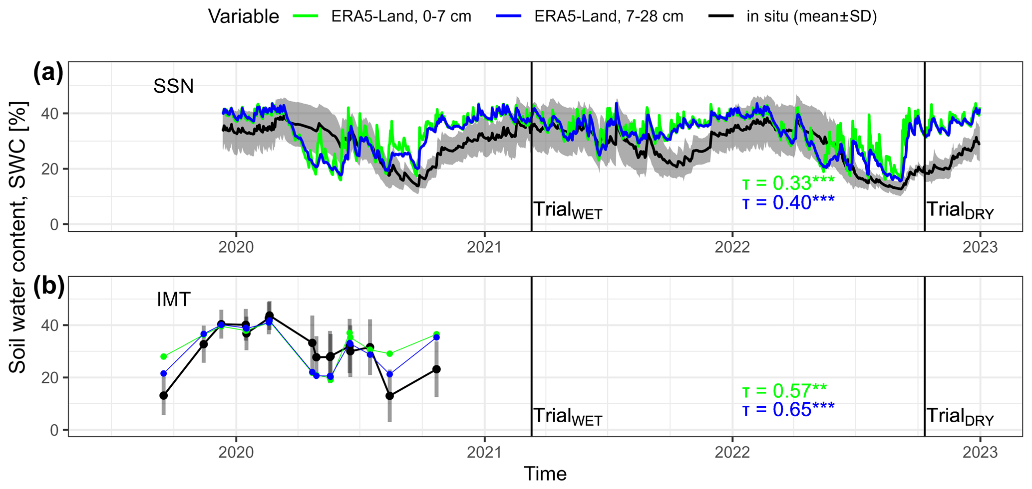
Figure 3 Time series of soil water content (SWC) measured using a soil sensor network SSN (a) with 18 measuring positions on two sites and manual measurements, using the impedance measuring technique IMT, (b) conducted on 252 positions (black lines/points show daily mean values; grey shading/bars show the standard deviation for each day). SWC retrievals from ERA5-Land are shown as a blue line/point (0–7 cm vertical resolution; as available from Copernicus Climate Change Service, 2019) and a green line/point (7–28 cm vertical resolution). The goodness of fit between daily means of measured SWC and ERA5-Land retrievals is reported using Kendall's rank correlation coefficient (τ). Vertical lines indicate the dates of the trials when a forwarder conducted four passes at existing machine-operating trails.

The eight-wheel machine trafficked sections 1 and 2 of both machine-operating trails and made four passes. Before the first machine pass, the initial surface was captured along 10 perpendicular transects on each of the four sections. These 4 m wide transects were placed and marked permanently with inserted wooden pegs. The same pegs were used to position the beam which served as the reference height to measure profiles along each transect. Metric scales were inserted into this beam with a spacing of 10 cm in between to note the distance between the surface and the beam to the nearest centimeter. These measured distances (D0; [cm]) describe the surface along the transect on already existing machine-operating trails prior to the trial conducted in this study. The same procedure was repeated after the fourth consecutive machine pass, giving D4 [cm].

Next, the differences between D0 and D4 were calculated at each of the 41 measurements (10 cm spacing over 4 m) along a transect. The maximum value of these differences, measured at the left or right machine track, was used to determine rut depth (RD; [cm]). We used average values of both tracks to prevent pseudo-replicates, since the intraclass correlation coefficient was high (0.83) when the left and right tracks were integrated separately. Moreover, mean and maximum values of rut depth were highly correlated (adj. R² = 0.96).

In total, 4 of the 40 transects for measuring RD were not ascertainable as the forwarder destroyed the wooden pegs that positioned the reference beam. In Trial_WET, conducted in March 2021, SWC_ERAL1 and SWC_ERAL2 showed a soil moisture level of 39 %. At Site A, the measured RD was 10.3 ± 1.9 cm, while at Site B, the RD was 12.7 ± 5.5 cm, with the highest value of RD recorded after four passes reaching a depth of 21.5 cm. In Trial_DRY, conducted in October 2022, the soil water content from ERA5-Land was 32 %. At Site A, the measured RD was 3.5 ± 1.7 cm, and at Site B, the RD was 4.3 ± 1.2 cm. Comparisons of RD with DTW and TWI are given in Fig. C1.

2.3.2 Soil water content at the rut depth transects (SWC_CORE)

Volumetric soil moisture content was captured outside the 1st, 4th, 7th, and 10th transect of each section, with a distance of 1 m to the left and right track at a depth of 10–15 cm. This water content was determined using 100 cm³ cores taken with an undisturbed core sampler with three replicates at each measurement. SWC_CORE was calculated according to Eq. (1):

$$\begin{array}{}\text{(1)}& {\mathrm{SWC}}_{\mathrm{CORE}}\left[\mathit{\%}\right]={\displaystyle \frac{\mathrm{M}\mathrm{2}-\mathrm{M}\mathrm{1}}{\mathrm{M}\mathrm{1}}}\cdot \mathrm{100},\end{array}$$

with M2 being the fresh mass of the soil taken with undisturbed cores, and M1 being the mass after drying the samples in oven at 105 °C until mass constancy was reached.

Measurements of RD and SWC_CORE were georeferenced using the GNSS device and complemented with all the predictor variables as described above.

2.4 Comparisons between model predictions and RD or SWC_CORE

For the “testing on rut depth data” (Fig. 1), values of SWC_PRED were compared to RD or SWC_CORE. The predictor variables from the rut depth data set were used to predict SWC_PRED by means of the final random forest models created in the soil moisture modeling. Since the goodness of fit between in situ values of RD or SWC_CORE and SWC_PRED was to some degree sensitive to the seed set during modeling, we repeated the predictions 10 times and used average values to receive robust estimates of SWC_PRED. To test the correlations between paired samples of SWC_CORE or RD and SWC_PRED, Kendall's rank correlation was used. We illustrated the corresponding p values with asterisks as follows: “${}^{***}$” for p<0.001, “${}^{**}$” for 0.001–0.01, “^*” for 0.01–0.05, “(^*)” for 0.05–0.10, and “ns” for p values higher than 0.10. The root mean squared error (RMSE) and mean squared error (MSE) were calculated according to Hamner and Frasco (2018). Values are given as mean ± standard deviation.

3 Results

3.1 Soil water content

The mean value of SWC, measured using a handheld moisture meter (IMT), varied between 13.0 ± 10.0 % in August 2020 and 43.2 ± 5.95 % in February 2020 (Fig. 3). Daily mean values obtained from soil sensor networks (SSNs) were similar to those obtained from IMT, ranging from 13.8 ± 2.90 % in September 2020 to 39.1 ± 6.66 % in March 2020, in the period that corresponds to the one covered by IMT. The driest conditions were observed in September 2022 with a daily mean SWC of 12.7 ± 2.55 %. Overall, the results suggest that IMT and SSN provide comparable estimates of SWC, with the latter providing higher temporal resolution at a low spatial granularity.

3.2 Soil moisture models

The position IDs were used to select the 10 folds for cross-validation. However, the data set SSN had only 18 measuring positions (where SWC was measured on 1116 d), resulting in relatively high deviations of Kendall's τ of the random forests. The most important feature for this data set was given by DTW025, although the resulting quality was low with τ of 0.363 ± 0.198. By adding the temporal component month, the τ improved to 0.637 ± 0.065, which had the lowest standard deviation for the repeated folds. The final model for this data set included the temporal variable month and SWC_ERAL2, as well as the topographic predictor variables TWI and DTW025 (Fig. 4). The resulting τ was 0.710 ± 0.095, which was revealed through the cross-validation.

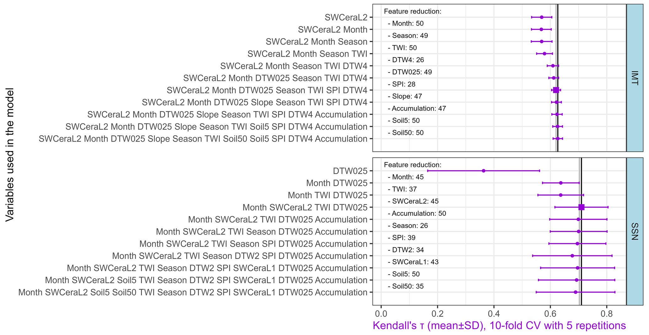
Figure 4 Soil water content (SWC) was modeled by random forests (RFs) and evaluated by a repeated 10-fold cross-validation (CV). Mean values and the standard deviation of the resulting values of the Kendall rank correlation coefficient τ during the CV are shown. A stepwise elimination of the least important variable was performed, and the frequency of this variable over all models is provided (“feature reduction”). The vertical lines indicate the maximum value of τ (black) and the 99 % value of the maximum (grey) used to select final models (squares). Variables used are described in Sect. 2.

For the IMT partition, which had a low temporal but high spatial resolution, the most important feature was the temporal information SWC_ERAL2, leading to τ of 0.569 ± 0.036. The final model had τ of 0.620 ± 0.016, including the predictor variables of SWC_ERAL2, month, season, DTW025, TWI, SPI, and DTW4.

The main outputs when both data sets were combined can be seen in Appendix A.

3.2.1 Comparisons of SWC_CORE with SWC_PRED

The final random forest models of both the IMT and SSN data set were used to calculate SWC_PRED on the predictor variables of the rut depth data. The comparison between SWC_CORE and SWC_PRED values predicted by the final random forest models of both data sets (SSN and IMT) revealed a significant association (Fig. 5).

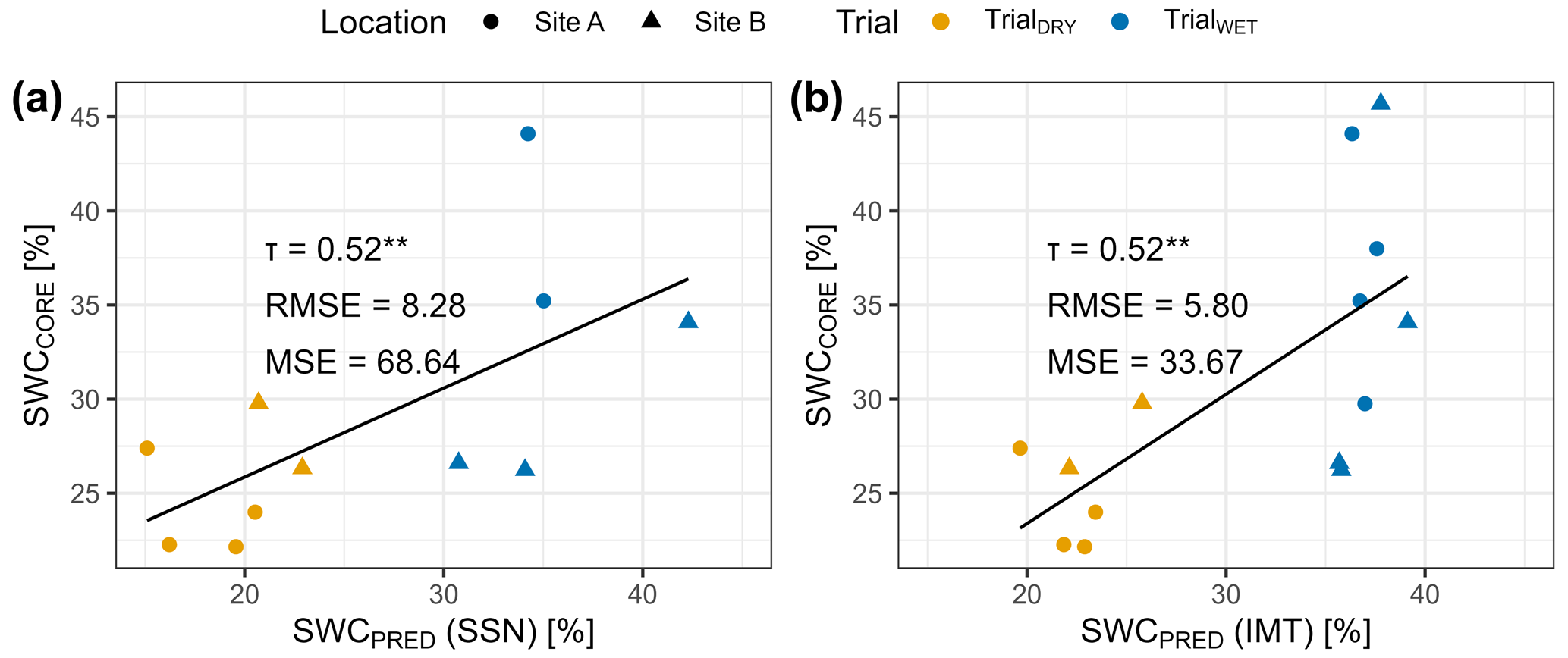
Figure 5 Soil water content was measured during two trials with a forwarder along a machine-operating trail (n=14), using 100 cm³ undisturbed cores (SWC_CORE), and compared to values predicted (SWC_PRED) by a model trained data from a continuously measuring soil sensor network (SSN; a) or manual measurements with a handheld moisture meter (IMT; b). Correlations were evaluated using Kendall's τ and significance levels are indicated by asterisks, with ${}^{***}$ for p<0.001, ${}^{**}$ for 0.001–0.01, ^* for 0.01–0.05, (^*) for 0.05–0.10, and “ns” for p>0.10.

3.3 Comparisons of RD with SWC_CORE and SWC_PRED

RD was positively correlated with SWC_CORE when both trials with different moisture conditions were included in testing (Fig. 6a). However, when each trial was tested separately, no correlation between RD and SWC_CORE was observed. Compared to the correlation between RD and SWC_CORE, modeling outputs SWC_PRED proved to be a better predictor of rut depth, particularly for Trial_WET. The final models that were selected for both data sets produced Kendall's τ of 0.61 (for IMT in Fig. 6b and SSN in Fig. 6c) when comparing RD of the four trials with the corresponding SWC_PRED. Although the R² values for these models were in a similar range (0.620 for IMT and 0.549 for SSN), we chose to use Kendall's τ since different sample sizes were involved in the analysis. This was particularly relevant for comparing RD with SWC_PRED for each trial separately. While no correlation could be found for Trial_DRY, correlations were found for Trial_WET, with Kendall's τ of 0.344 (p=0.037) and 0.281 (p=0.090), and for the final models trained on IMT and SSN, respectively (Fig. 6b, c). Yet, these correlations seem fragile as a difference of a few percent of predicted SWC_PRED (IMT) is associated with the range of RD between 6.5 and 21.5 cm. Moreover, when analyzing the sites separately, a vague trend between SWC_PRED and RD could be observed but without showing significant correlations (Fig. B1).

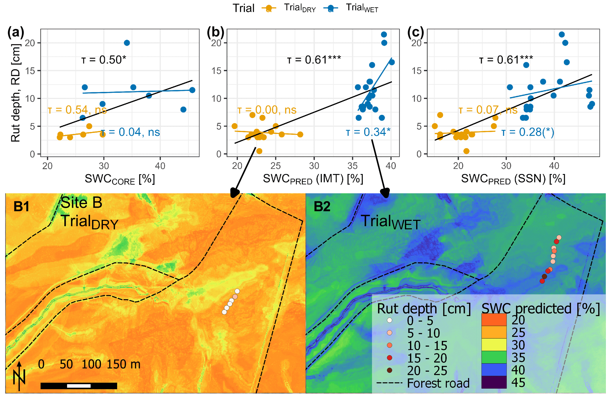
Figure 6 Rut depth (RD) was determined after four passes of a forwarder driving on two sites during two conditions (WET and DRY). RD was compared to SWC values determined for undisturbed soil cores (a) and SWC values predicted by a random forest model trained on manually obtained IMT measurements (b; see Fig. 1) and predicted by a model trained on data from a continuously measuring soil sensor network (SSN; c). Correlations were evaluated using Kendall's τ. The correlation of all values is given in black; blue and yellow show the trials during wet and dry conditions. Significance levels are indicated by asterisks, with ${}^{***}$ for p<0.001, ${}^{**}$ for 0.001–0.01, ^* for 0.01–0.05, (^*) for 0.05–0.10, and “ns” for p>0.10. The model based on IMT data (b) was used to calculate prediction rasters for the days of the field trials (B1 and B2).

Since the final model trained on IMT data performed slightly better in Trial_WET compared to the model trained on SSN data (Fig. 6), we chose the IMT model for the generation of prediction rasters for the days of interest (Fig. 6B1, B2).

4 Discussion

4.1 Importance of predictive systems

Wet soils are prone to soil disturbances like the formation of deep ruts (Poltorak et al., 2018; McNabb et al., 2001), since water implies a reduction in the particle-to-particle bonding within the soil (Hillel, 1998), decreasing the resistance to external forces. Consequently, accurate predictions of soil water content (SWC) and soil trafficability are essential for sustainable forest management and cost-effective, environmentally friendly harvesting operations (Vega-Nieva et al., 2009; Mattila and Tokola, 2019; Picchio et al., 2020; White et al., 2012; Murphy et al., 2007; Mohtashami et al., 2017; Uusitalo et al., 2020). Topographic modeling requires minimal input, and the temporal variables used in the final model presented here are freely available (Copernicus Climate Change Service, 2019). A spatiotemporal model predicting SWC could improve the guidance for machine operators in forest sites during harvesting operations, for example, by the effective positioning of brush mats (Labelle et al., 2019; Labelle and Jaeger, 2018). Practical use of static topographic maps has already been observed in Canada and Scandinavian countries (Ring et al., 2022). By incorporating a temporal aspect, the accuracy of these tools could be further improved. This has the potential to enhance sustainable forest management by protecting soil and mitigating harmful sediment transport (Ågren et al., 2015; Lidberg et al., 2020; Kuglerová et al., 2017; White et al., 2012).

4.2 Comparison to previous work on predictions of SWC

Since soil moisture predictions are crucial for a variety of forestry aspects, several publications have focused on this topic before. For example, Lidberg et al. (2020) predicted soil moisture classes using spatial models built on topographic indices, correctly classifying 73 % of wet areas in a Swedish case study. Ågren et al. (2014) reported accurate predictions for 87 %–92 % of observations by comparing soil moisture classes to DTW maps. Larson et al. (2022) used data from the Krycklan catchment and found an accuracy of 84 % when comparing moisture classes to the recently developed “SLU soil moisture map” (Ågren et al., 2021). However, these validations were based on static topographic maps. One attempt to make such static maps dynamic was realized within the DTW concept which can be customized to calculate various scenarios to adjust to general moisture conditions (e.g., flow initiation areas of 0.25, 1, and 4 ha for wet, moist, and dry conditions, respectively), but selecting the most appropriate scenario during practical use can be a challenging task that requires significant expertise (White et al., 2012; Lidberg et al., 2020; Leach et al., 2017). To overcome this challenge, we aimed for the improvement of soil moisture prediction and refined the spatiotemporal approach conceived by Schönauer et al. (2022). During the cross-validation of IMT data from sites in Finland, Poland, and parts of the data used in this work, they reported an R² of 0.80. The models for the present study showed an R² of 0.759 ± 0.136 (SSN) or 0.636 ± 0.040 (IMT), corresponding to Kendall's τ of 0.710 ± 0.095 or 0.620 ± 0.016, respectively. Although this may not seem like an improvement, it should be noted that the data from German sites had less explanatory power for the topography when predicting SWC. For example, DTW4 alone explained SWC to a very limited extent (R² = 0.037${}^{***}$).

4.3 Prediction of rutting

Besides the comparisons of SWC with DTW maps, various studies have also investigated the capability of topographic indices to predict rutting – with conflicting outcomes. For example, Vega-Nieva et al. (2009) found that 65 % of ruts deeper than 25 cm were located in areas with a DTW value smaller than 1 m, and 93 % of these ruts occurred in areas with DTW values smaller than 10 m. Similarly, Heppelmann et al. (2022) observed a high frequency of severe rut depth in areas with DTW values smaller than 1 m in Norway. However, Mohtashami et al. (2017) did not find evidence of such patterns in a field trial where the inclusion of DTW values did not improve the accuracy of a linear model to describe the extents and degrees of rut depth on machine-operating trails. In agreement, Schönauer et al. (2021a) found no evidence that DTW or TWI could predict rut depth in a field trial conducted in a temperate broadleaved stand. In this study, we found a significant correlation between RD and DTW025 with Kendall's correlation coefficient (τ) of −0.52${}^{***}$. Yet, this correlation has to be viewed with caution. It is mainly driven by differing ranges of RD between the two trials, as can be seen in Fig. C1a. We observed that the temporal adjustments of the model based on current moisture conditions improved predictions of rutting by up-to-date SWC predictions, leading to τ of 0.61${}^{***}$ (Fig. 6b, c). While a strong association between RD and predicted values of SWC was observed, the influence of the differences between the trials is evident. However, the ranges of RD for each trial were consistent with the SWC predictions. In Trial_WET, a significant correlation between RD and SWC_PRED was observed (Fig. 6b). We hypothesize that the wetter conditions during this trial, which lead to soil destabilization (Hillel, 1998; McNabb et al., 2001), enhanced the predictive power of topographic indices representing soil water distributions. For instance, DTW025 overlapped with surface water in depressions, as observed in the field campaigns for Trial_WET.

In contrast, during Trial_DRY, no correlation was found between RD and SWC_PRED. SWC along the measuring sections was likely below the threshold for soils to become susceptible to deformation. For example, Poltorak et al. (2018) stated that ruts only occurred on soils with SWC above 50 %, whereas SWC_CORE at Trial_DRY was below 30 % (Fig. 5).

4.4 Description of the model

The best-performing model for predicting RD incorporated temporal information from SWC_ERAL2, month, and season, as well as spatial information from DTW025, TWI, SPI, and DTW4 and was based on data from the manual measurements (IMT). The IMT data were collected in close proximity to the rut depth measurements at Site A (Fig. 2) or with a distance of up to 1.3 km at Site B. However, the spatial distance between the IMT training data and the rut depth data did not seem to be crucial for the accuracy of predicting rut depth (Fig. B1), since Kendall's τ between RD and SWC_PRED was similar for both sites. Surprisingly, in situ SWC_CORE, sampled directly at the machine-operating trails, showed a lower explanatory power in predicting RD than SWC_PRED. Although an overall association was confirmed, no correlation could be found when trials were analyzed individually.

4.4.1 Temporal variation was more important than spatial variation

The lacking association between RD and SWC_CORE on individual trials indicates that the temporal variability in soil moisture between the trials was more important in this study than the spatial variability within the relatively small areas where each trial was conducted. The spatial distribution of the rut depth measurements might have been limiting in the present work. The semivariogram indicates the spatial covariation of rut depth and SWC (Fig. 7). While the covariation of RD in Site A is indicated to be high within a range of 10 m (RD transects were at this distance), on Site B, during wet conditions, the sill of the semivariogram reaches almost 40 m, which covered a high number of transects. Similarly, excluding soil information in the initial stages of feature reduction suggests homogeneous soil properties in the relatively small study area.

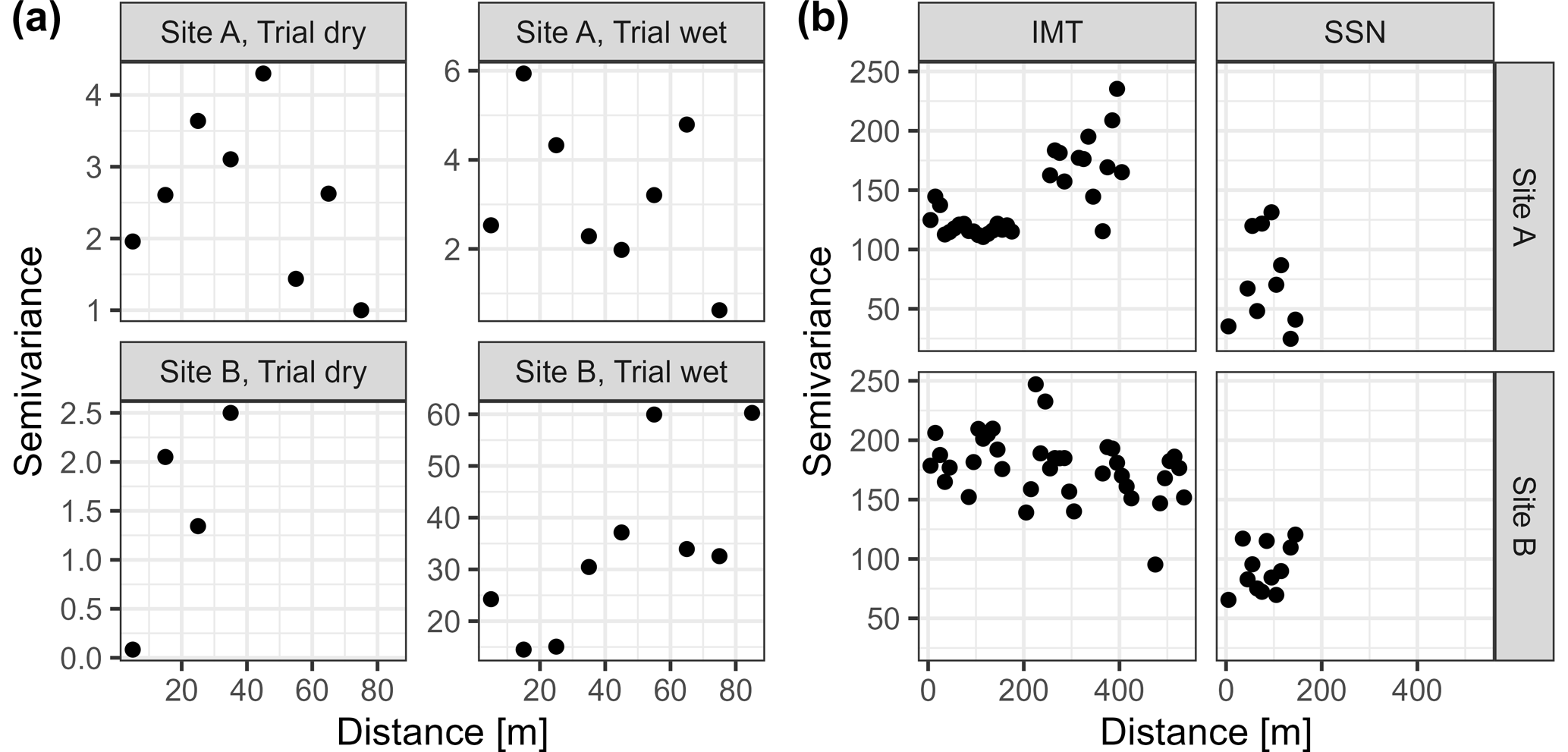
Figure 7 Semivariogram illustrating spatial autocorrelation of (a) rut depth (cm) and (b) soil water content (SWC) across the study area. Rut depth was measured during two moisture conditions at four machine-operating trail sections allocated on two sites. The measuring transects had a spacing of 10 m. SWC was measured with handled measuring techniques (IMT) or a soil sensor network (SSN) (Fig. 2).

Therefore, we have to admit that the study design was not ideal for assessing the ability to predict rutting with a spatiotemporal model of SWC, and the results have to be considered with caution.

The spatiotemporal model (IMT), also supports the conclusion that spatial variations were either underrepresented by the study design or very low compared to temporal variation by nature, as the temporal feature SWC_ERAL2 was selected as the most important variable, and the difference between the model with one predictor variable vs. the final model was small (Fig. 4).

Still, this slight increase in the models' quality allowed the integration of spatial patterns and resulted in the significant but vague prediction of RD in Trial_WET (τ= 0.344^*; Fig. 6). Another indication of the integration of spatial patterns can be interpreted from the segregation of the temporal range of the IMT data (2019–2020) and the actual trials (March 2021 and October 2022; Fig. 3) which indicate a generalization of spatial and temporal patterns.

4.4.2 Most important variables

In the final model (IMT), SWC_ERAL2 has been identified as the most important variable, followed by the month and season. It is noteworthy that in the data with broader spatial coverage (i.e., IMT), in contrast to the SSN data, dynamic variables took precedence over predictor variables. Surprisingly, when modeling SSN data characterized by a high temporal resolution and low spatial resolution, DTW025 remained the most influential variable. One might have anticipated the opposite, expecting a topographic index to play a central role in modeling IMT data and dynamic SWC_ERA variables to dominate the modeling of SSN data.

We presume that the low spatial variations in the SWC in comparison to temporal variations, inadequately represented by the provided topographic information, may have contributed to this unexpected outcome. Furthermore, the wider spatial coverage in the IMT data likely resulted in more robust averages of SWC, leading to a stronger correlation with the coarse spatial data of ERA5-Land (9 × 9 km). On the contrary, the spatial distribution of the SSN data, originating from areas with a size of 100 × 100 m and known for their temporal wetness, could explain the heightened importance of DTW025. Some sensors might have measured constant water saturation, thereby inflating the explanatory power of topographic information. These assumptions are speculative, and further research in this direction is warranted.

In the feature reductions in the IMT and SSN data (Fig. 4), SWC_ERAL2 (7–28 cm soil depth) dominated over SWC_ERAL1 (0–7 cm). This aligns with in situ measurements of SWC by the SSNs conducted at soil depths of approximately 10 cm (Fig. 3a). Even for the IMT data, where SWC was measured in the top 6 cm of soil, SWC_ERAL2 yielded a better goodness of fit compared to SWC_ERAL1 (Fig. 3b). We hypothesize that the prevalence of open lands as the dominant land cover form in the ERA5-Land raster cell (Sect. 2.2.4) contributed to the superior fit of SWC_ERAL2. Grasslands typically exhibit higher temporal heterogeneity of soil moisture compared to forests (James et al., 2003). This temporal heterogeneity tends to decrease with deeper soil layers (Tromp-van Meerveld and McDonnell, 2006). Therefore, the stronger correlation between SWC_ERAL2 and SWC, as well as its higher importance within the random forests, seems reasonable. The disparity between SWC_ERA and in situ SWC can be attributed to the high transpiration rates in forests as opposed to grasslands (Kelliher et al., 1993).

4.5 Further developments

The terrain data were derived from a digital elevation model, which is increasingly available for the entire Europe (Hoffmann et al., 2022), while the dynamic variables are based on date and retrievals from ERA5-Land, which are freely available up to a few days ago. These inputs would allow automated mapping of current soil water content, which could be made accessible to forestry stakeholders. Recent developments also show a pathway to integrate medium- and long-range weather forecasts into trafficability predictions, as conceived by the Finnish Meteorological Institute (2023). Both recent and forecasting predictions can lead to improved soil protection, higher efficiency of timber harvesting (Suvinen and Saarilahti, 2006), and a new stage of sustainable forest management (Campbell et al., 2013; D'Acqui et al., 2020; Uusitalo et al., 2019; Jones and Arp, 2019). However, it should be noted that the in situ data of SWC originated from manual measurements, and it was relatively labor-intensive to gather this amount of data. There is the potential to reach appropriate accuracy, even with a reduced data set; further investigation would be necessary to determine the essential input data criteria. The alternative to manual measurements is given by sensor networks which led to comparable results but are expensive to establish and maintain. Nonetheless, initiatives for installing sensors are emerging, and additional manual measurements could be conducted. In the future, forestry stakeholders who require accurate raster predictions could potentially facilitate manual measurements or install sensors and provide the captured data to scientific organizations which could deliver spatiotemporal soil moisture predictions in return. The captured data could be made available for creating spatiotemporal models of SWC, allowing additional training data and daily raster predictions for new areas of interest and with various scientific insights and practical applications.

5 Conclusion

In this study, we developed a spatiotemporal model that used multiple topographic indices, temporal variables, soil moisture retrievals from ERA5-Land, and data from manual measurements to predict soil water content (SWC). Predicted values of SWC were compared to rut depth data collected during four forwarder trials. Overall, the model performed well in predicting rut depth, with Kendall's τ of 0.61 for all trials. Yet, this result has to be considered with caution, since spatial covariation was detected in parts. We hope that this experience helps for future research in which more attention to spatial covariation on soils should be paid. Still, we believe that a dynamic prediction of SWC will help forest managers and machine operators avoid wet areas, leading to more sustainable forest operations. Using freely available temporal information is a significant improvement, as it enables more accurate and up-to-date predictions which allow us to make more informed decisions and avoid potential hazards. Future work should focus on developing automated pathways for generating daily raster predictions of SWC and on generating reliable and comprehensive in situ data. There is a need for more data on rutting and SWC that are measured with a sufficient spatial coverage, whether by manual measurements, the establishment of additional sensor networks, or by automatic ways of capturing rut depth data through machines driving off-road to cover more areas and different sites and regions.

Appendix A

To model the data set consisting of both IMT and SSN data, the procedure described in Sect. 2 was followed. The IMT data set was merged with a subsample of the SSN data set, where the sample size of the SSN part was twice that of the IMT data set. This was done to prevent the overweighting of the SSN data set. The resulting combination of IMT and SSN data was called the “Mix” data set.

The final model using the Mix data set included the input variables SWC_ERAL2, month, TWI, SWC_ERAL1, DTW025, season, DTW1 and DTW4, and achieved τ of 0.655 ± 0.081 (which corresponded to R² values of 0.639 ± 0.108). Figure A1 shows that the correlation between the model outputs (SWC_PRED) and rut depth (RD) was significant.

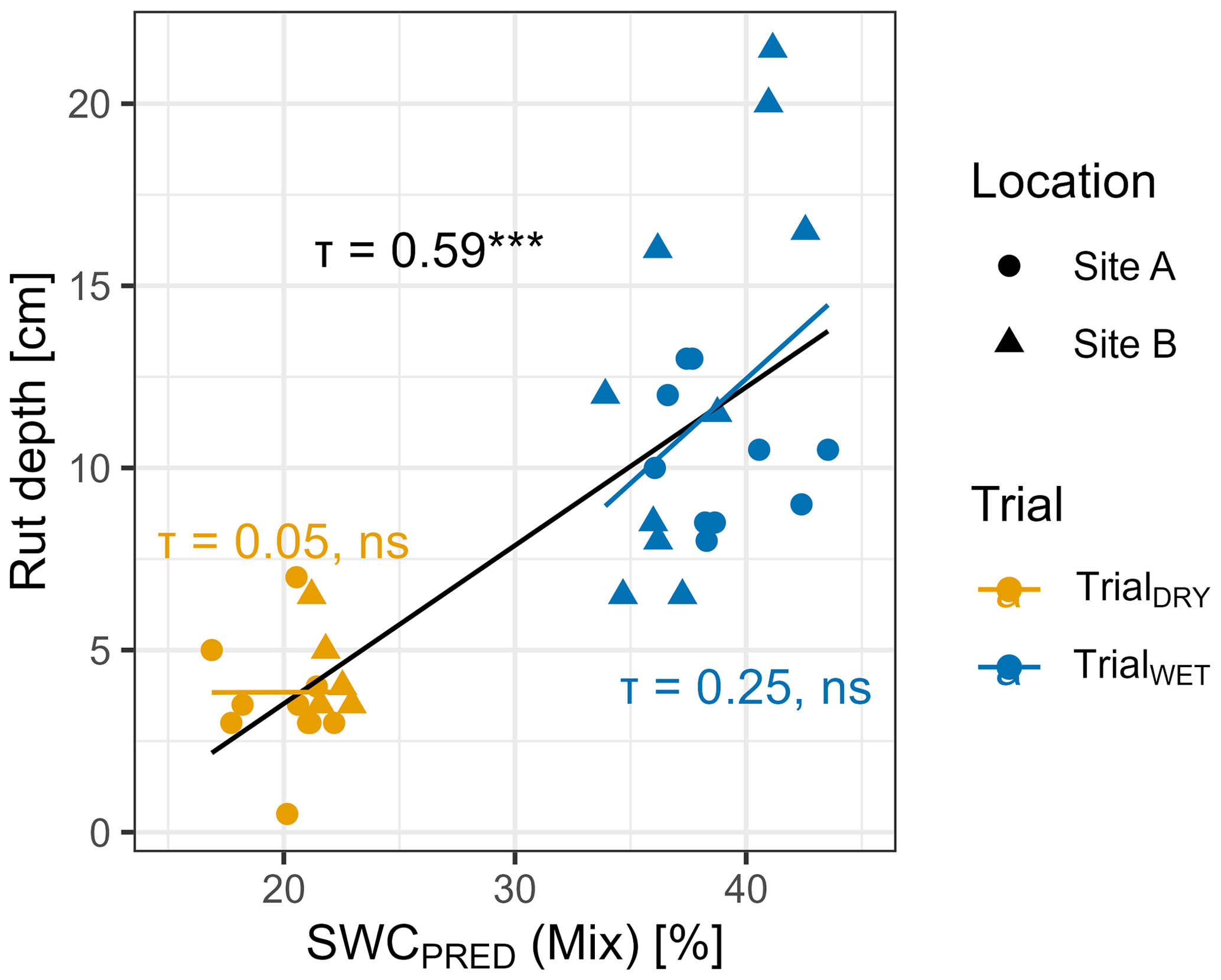
Figure A1 Rut depth (RD) was determined after four passes of a forwarder, driving on two Sites (A and B), during two seasons (Trial_WET and Trial_DRY). RD was compared to SWC values predicted by a random forest model trained on data from manual measurements or captured through a continuously measuring soil sensor network (“Mix”). Correlations were evaluated using Kendall's τ, and significance levels are indicated by asterisks, with ${}^{***}$ for p<0.001, ${}^{**}$ for 0.001–0.01, ^* for 0.01–0.05, (^*) for 0.05–0.10, and “ns” for p>0.10.

Since the models trained on the Mix data set did not perform better than those trained on the IMT or SSN data sets, we did not investigate the fused data partition any further, as one research question addressed the use of different data origins. For future work, however, the fused data would provide additional information compared to the individual data sets.

Appendix B

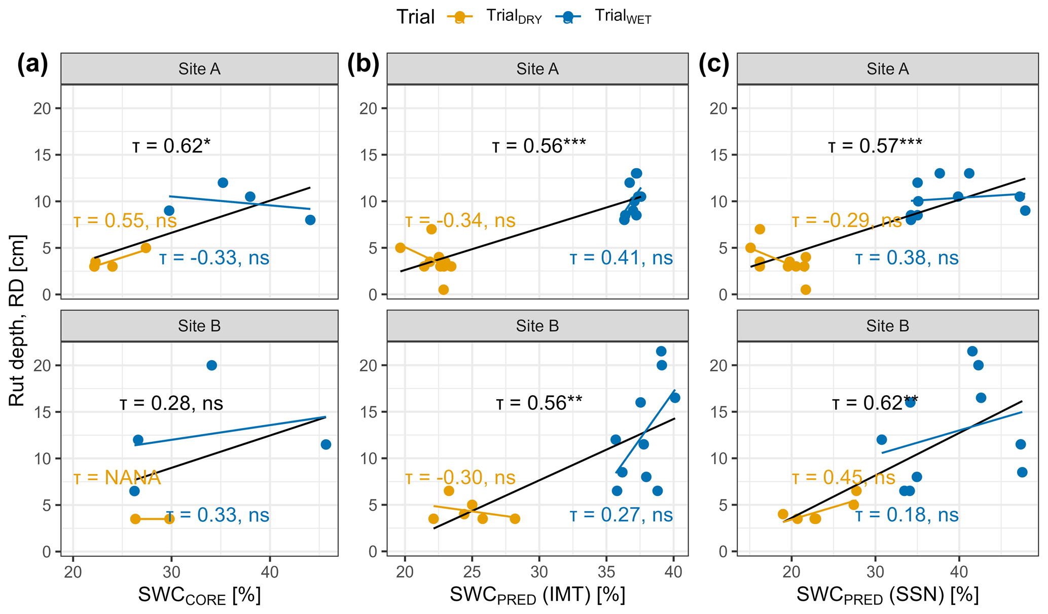
Figure B1 Rut depth (RD) was determined after four passes of a forwarder driving on two Sites (A and B; Fig. 2) during two seasons (Trial_WET and Trial_DRY; conducted under different moisture conditions). RD was compared to SWC values determined for undisturbed soil cores (a) and SWC values predicted by a random forest model trained on manually obtained IMT measurements (b; see Fig. 1) and predicted by a model trained data from a continuously measuring soil sensor network (SSN; c). Correlations were evaluated using Kendall's τ. The correlation of all values is given in black; blue and yellow show the trials during wet and dry conditions. Significance levels are indicated by asterisks, with ${}^{***}$ for p<0.001, ${}^{**}$ for 0.001–0.01, ^* for 0.01–0.05, (^*) for 0.05–0.10, and “ns” for p>0.10.

Appendix C

Considering the significance of the topographic indices DTW and TWI in the development of the SWC models (Fig. 4), we aimed to compare RD with both indices. Notably, RD exhibited a clear correlation with DTW025, the most conservative DTW scenario (Fig. C1). TWI also demonstrated a correlation with RD.

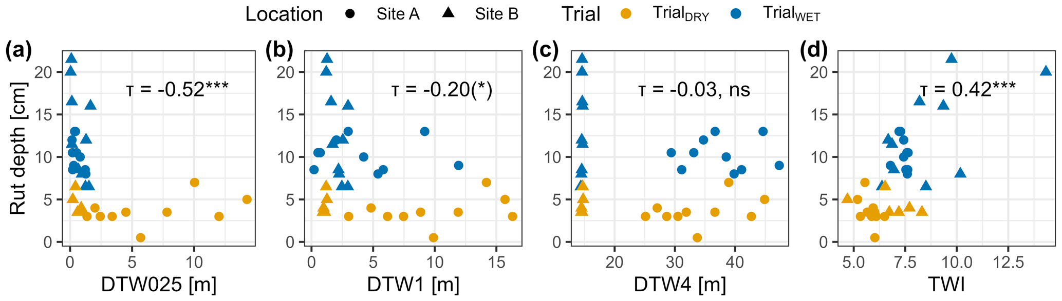
Figure C1 Rut depth (RD) was determined after four passes of a forwarder driving on two Sites (A and B) during two conditions (Trial_WET and Trial_DRY). RD was compared to the topographic indices depth-to-water (DTW), calculated with different flow initiation areas (0.25–4.00 ha), and the topographic wetness index. Correlations were evaluated using Kendall's τ, and significance levels are indicated by asterisks, with ${}^{***}$ for p<0.001, ${}^{**}$ for 0.001–0.01, ^* for 0.01–0.05, (^*) for 0.05–0.10, and “ns” for p>0.10.

While showing significant correlations, the nature of these static maps does not allow for the representation of current moisture conditions. This limitation was overcome when using the predicted (or observed) values of SWC.