Technical note: Isotopic fractionation of evaporating waters: effect of sub-daily atmospheric variations and eventual depletion of heavy isotopes

Isotopic fractionation of evaporating waters has been studied constantly in recent decades, particularly because it enables calculation of both the volume of water evaporated from a water body and the isotopic composition of its source water. We studied the stable water isotopic composition of an artificial pan filled with water and subject to total evaporation in a sub-humid environment, in order to put into practice an operational method for estimating the time since disconnection of riverine pools when these are sampled for the quality of aquatic life.

Results indicate that (i) when about 70 % of pan water had evaporated and its isotopic composition had become enriched in heavy isotopes, some subsequent periods of depletion instead of enrichment happened; and (ii) the customary application of isotopic fractionation equations to determine the isotopic composition of the water in the pan using weekly averaged atmospheric conditions (temperature and relative humidity) strongly underestimated the changes observed but predicted an early depletion of heavy isotopes. The first result, rarely reported in the literature, was found to be fully consistent with the early studies of the isotopic composition of evaporating waters. The second one could be attributed to the fact that weekly averages of temperature and relative humidity strongly overestimated air relative humidity during daylight periods of active evaporation. However, when the fractionation equations were parameterized using temperature and relative humidity weighted by potential evapotranspiration at sub-hourly time steps, they adequately reproduced the observed isotopic composition of the water in the pan, including the late periods of heavy isotope depletion.

We demonstrate how weekly increases in air relative humidity when the pan water was already enriched in heavy isotopes led to their depletion. We also analyse the errors that can be incurred if time averages are used instead of flux-weighted meteorological data for model parameterization and if unidentified periods of heavy isotope depletion occur. Our results should be taken into account when applying fractionation equations, particularly in conditions or areas with high air relative humidity.

1 Introduction

There is increasing interest in the use of stable isotopes in open, soil, and xylem waters to study either the volume of evaporated water or the original composition of the source water. The following articles synthesized published studies of open water (Skrzypek et al., 2015), of soil and vegetation (Benettin et al., 2018), and of rainfall interception processes (Allen et al., 2017). Several authors recommended using temperature and relative humidity weighted by the evaporation flux for fractionation studies (e.g. Allison and Leaney, 1982; Gibson, 2002; Gibson et al., 2008, 2016). However, in practice this recommendation is not usually followed (except, for example, Mayr et al., 2007), particularly where air humidity is low (e.g. Hamilton et al., 2005; Skrzypek et al., 2015) or when monthly or seasonal periods are investigated (e.g. Benettin et al., 2018).

During evaporation of water in a natural environment, lighter water molecules usually vaporize more quickly than heavier ones, so that the remaining water body becomes enriched in heavier isotopes (Craig et al., 1963). However, heavy isotope concentrations in water evaporating into open air with moderate or high relative humidity increase asymptotically to a stationary isotopic state, establishing a dynamic equilibrium as the mass of water decreases to zero. This effect is attributed to a rapid molecular exchange of isotopes between the water body and the atmospheric vapour, which predominates over the net isotopic effect of a simple evaporation process (Craig et al., 1963). Isotopic exchange that induces depletion rather than enrichment in heavy isotopes of the evaporating water has been identified, for example, in canopy interception processes, when air humidity is near saturation (Saxena, 1968; Allen et al., 2017).

Gonfiantini (1986) showed that stationary or limiting isotopic composition (δ^*) depends mainly on air relative humidity to the extent that, when air relative humidity is low, δ^* concentrations are practically unreachable, whereas, when it approaches 95 %, these can be reached when only about 20 % of water has evaporated.

Most temporary rivers, from the cessation of flow to the total desiccation of the river bed, undergo a disconnected pool phase (Gallart et al., 2017). As the aquatic life in these pools naturally changes after the flow cessation (Bonada et al., 2020), the time between disconnection of these pools and sampling is information needed for assessing their biological quality. To implement an operational procedure to estimate the time since disconnection of river pools, based on the study of water stable isotopes, an artificial pan was set up and subjected to evaporation to complete dryness in a location with a sub-humid climate, as a counterweight to the more frequent studies in dry climates.

The purpose of this technical note is to describe and analyse the occurrence of periods of heavy isotope depletion instead of enrichment during evaporation of water in an artificial pan and the validation of the Gonfiantini (1986) equation in predicting both the enrichment and depletion in heavy isotopes of evaporating waters. In addition, we describe the environmental conditions that induced depletion instead of enrichment in heavy isotopes of the evaporating water, and we also analyse the likely errors that can be incurred in studies of the isotopic composition of evaporating water if the meteorological data are time-averaged instead of flux-weighted, as well as when periods of heavy isotope depletion occur during water evaporation.

2 Data and methods

The experiment was performed in the Vallcebre research catchments (eastern Pyrenees, Iberian Peninsula). The climate is sub-humid Mediterranean, the mean temperature is 9.1 ^∘C, the mean annual precipitation is 880 mm, and the mean annual potential evapotranspiration is 818 mm (Llorens et al., 2018).

A round steel pan (Fig. 1) was filled with 70 L of water from a nearby spring, partly buried in the ground and protected against precipitation by a lid of clear methacrylate installed 0.5 m above the pan's surface, to allow air circulation. A net stopped animals from drinking. Bulk rainfall was sampled with a 180 mm diameter funnel connected to a 1 L plastic bottle with a pipe with a loop to prevent evaporation.

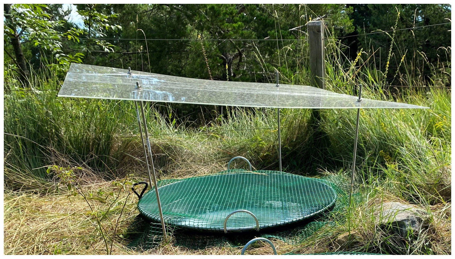
Figure 1 View of the steel experimental pan. The pan was partly buried in the ground and protected against precipitation by a lid of clear methacrylate installed 0.5 m above the pan's surface, to allow air circulation, and against large animals drinking by a net.

Every week from June to October 2020, until the pan had practically dried out (19 weeks), the volume of water in the pan was recorded and water samples were taken from the pan and bulk rain for isotopic analyses.

Air temperature (T) and relative humidity (h) (Vaisala, Finland), net radiation (Kipp and Zonen, the Netherlands), and wind speed (Thies Clima, Germany) were measured every 10 s and recorded at 5 min intervals by a data logger (Data Taker, Australia) in a meteorological station adjacent to the sampled pan.

Water samples were analysed for their stable isotope ratios (¹⁸O and ²H) via cavity ring-down spectroscopy (Picarro L2120-i, Picarro Inc., USA) at the laboratory of the Centre of Hydrogeology, University of Málaga. The precision of the isotope ratio measurements was reported as <0.1 ‰ for δ¹⁸O and <0.4 ‰ for δ²H. The data were expressed in δ notation as parts per mil (‰) relative to Vienna Standard Mean Ocean Water (VSMOW).

The isotopic composition (δ_L, ‰) of the residual water in the pan was modelled weekly for ¹⁸O and ²H, as in Gonfiantini (1986):

$$\begin{array}{}\text{(1)}& {\mathit{\delta }}_{\mathrm{L}}=\left({\mathit{\delta }}_{\mathrm{0}}-{\mathit{\delta }}^{*}\right)(\mathrm{1}-x{)}^m+{\mathit{\delta }}^{*},\end{array}$$

where δ₀ is the initial or modelled isotopic composition for the end of the previous week, δ^* is the stationary or limiting isotopic composition reached when the remaining water in a pool tends to 0, m is the slope of the temporal enrichment (Gibson et al., 2016), and x is the fraction of the water volume that evaporated. Thus, 1−x is the residual volume fraction. It is worth emphasizing that this equation does not require that evaporation induces an increase in δ_L with respect to δ₀ (enrichment) but that δ_L approaches δ^* in either direction (enrichment or depletion).

The coefficients of Eq. (1) were calculated as follows:

$$\begin{array}{}\text{(2)}& {\displaystyle }& {\displaystyle }{\mathit{\delta }}^{*}={\displaystyle \frac{\left(h{\mathit{\delta }}_{\mathrm{A}}+{\mathit{\epsilon }}_{\mathrm{k}}+{\mathit{\epsilon }}^{+}/{\mathit{\alpha }}^{+}\right)}{\left(h-{\mathrm{10}}^{-\mathrm{3}}\cdot \left({\mathit{\epsilon }}_{\mathrm{k}}+{\mathit{\epsilon }}^{+}/{\mathit{\alpha }}^{+}\right)\right)}},\text{(3)}& {\displaystyle }& {\displaystyle }m={\displaystyle \frac{\left(h-{\mathrm{10}}^{-\mathrm{3}}\cdot \left({\mathit{\epsilon }}_{\mathrm{k}}+{\mathit{\epsilon }}^{+}/{\mathit{\alpha }}^{+}\right)\right)}{\left(\mathrm{1}-h+{\mathrm{10}}^{-\mathrm{3}}\cdot {\mathit{\epsilon }}_{\mathrm{k}}\right)}},\end{array}$$

where h (–) is the relative humidity, δ_A (‰) is the isotopic composition of the atmospheric moisture, ε_k (‰) is the kinetic fractionation factor, ε⁺ (‰) is the isotopic separation between liquid and vapour, and α⁺ (‰) is the equilibrium fractionation factor.

δ_A was assumed to be in equilibrium with the isotopic composition of precipitation δ_P and was calculated as in Gibson et al. (2008):

$$\begin{array}{}\text{(4)}& {\mathit{\delta }}_{\mathrm{A}}=\left({\mathit{\delta }}_{\mathrm{P}}-{\mathit{\epsilon }}^{+}\right)/{\mathit{\alpha }}^{+}.\end{array}$$

ε_k was calculated as in Gat (1996) and Horita et al. (2008):

$$\begin{array}{}\text{(5)}& {\mathit{\epsilon }}_{\mathrm{k}}=\mathit{\theta }n(\mathrm{1}-h)\left(\mathrm{1}-D_{\mathrm{i}}/D\right){\mathrm{10}}^{\mathrm{3}},\end{array}$$

where θ is a weighting term that can be assumed to be equal to 1 for a small body of water whose evaporation flux does not perturb the ambient moisture significantly (Gat, 1996). The factor n, which accounts for the aerodynamic regime above the evaporating liquid–vapour interface, was assumed to be 0.5 (turbulent) as for an open water body. $D_{\mathrm{i}}/D$ is the diffusivity ratio between light and heavy isotopes. Following Merlivat (1978), $D_{\mathrm{i}}/D$ is 0.9755 and 0.9723 for ²H and ¹⁸O, respectively.

ε⁺ was obtained from

$$\begin{array}{}\text{(6)}& {\mathit{\epsilon }}^{+}=\left({\mathit{\alpha }}^{+}-\mathrm{1}\right){\mathrm{10}}^{\mathrm{3}},\end{array}$$

where α⁺ is calculated from the absolute temperature T (K), as in Horita and Wesolowski (1994):

$$\begin{array}{}\text{(7)}& \begin{array}{rl}{\mathrm{10}}^{\mathrm{3}}\ln & \left({\mathit{\alpha }}^{+}\right)=\mathrm{1158.8}\left(T^{\mathrm{3}}/{\mathrm{10}}^{\mathrm{9}}\right)-\mathrm{1620.1}\left(T^{\mathrm{2}}/{\mathrm{10}}^{\mathrm{6}}\right)\\ & +\mathrm{794.84}\left(T/{\mathrm{10}}^{\mathrm{3}}\right)-\mathrm{161.04}+\mathrm{2.9992}\left({\mathrm{10}}^{\mathrm{9}}/T^{\mathrm{3}}\right)\end{array}\end{array}$$

for ²H, and

$$\begin{array}{}\text{(8)}& \begin{array}{rl}{\mathrm{10}}^{\mathrm{3}}\ln \left({\mathit{\alpha }}^{+}\right)& =-\mathrm{7.685}+\mathrm{6.7123}\left({\mathrm{10}}^{\mathrm{3}}/T\right)\\ & -\mathrm{1.6664}\left({\mathrm{10}}^{\mathrm{6}}/T^{\mathrm{2}}\right)+\mathrm{0.3504}\left({\mathrm{10}}^{\mathrm{9}}/T^{\mathrm{3}}\right)\end{array}\end{array}$$

for ¹⁸O.

As we observed some significant periods of heavy isotope depletion in the pan water, we analysed the light isotope balance to investigate the net mass fluxes, i.e. to verify whether these isotopes had evaporated rather than condensed throughout the event. For this purpose, the mass of water in moles M_w was obtained for every visit from its volume using a density of 0.9976 kg L⁻¹ and a molar mass of 18.015 g per mole. Small changes in these values due to the variation in heavy isotope concentrations were not taken into account because they are mutually cancelled out.

Then, R_sa sample isotope ratios were obtained for each of the two heavy isotopes from the corresponding δ values:

$$\begin{array}{}\text{(9)}& R_{\mathrm{sa}}=(\partial /\mathrm{1000}+\mathrm{1})\cdot R_{\mathrm{st}},\end{array}$$

where R_st are the isotopic ratios of the VSMOW standards, which were taken as $\mathrm{1}/\mathrm{6420}$ for ²H and $\mathrm{1}/\mathrm{498.7}$ for ¹⁸O. Finally, the mass in moles of the light isotopes M_l were obtained for every sample and isotope using

$$\begin{array}{}\text{(10)}& M_{\mathrm{l}}=M_{\mathrm{w}}\cdot \mathrm{na}/\left(\mathrm{1}+R_{\mathrm{sa}}\right),\end{array}$$

where “na” is the number of atoms in each water molecule: one for oxygen and two for hydrogen.

As time-averaged meteorological variables were largely biased due to the diel variations (lower temperature and higher relative humidity during the night, when evaporation is lowest), flux-weighted daily and weekly T and h values were obtained by weighting sub-hourly readings with the corresponding evaporative flux calculated using the Penman–Monteith equation parameterized as for the reference evapotranspiration (Allen et al., 1998). A pan coefficient was not necessary because it cancelled out during weighting. Subsequently, the results obtained with time-averaged meteorological variables are labelled “unweighted” and those obtained by potential evapotranspiration (PET) weighting are labelled “weighted” or are unlabelled.

We first applied the Gonfiantini (1986) Eq. (1) to simulate pan water isotopic composition from observed volume changes, using unweighted and weighted meteorological conditions and allowing analysis of errors in both parameterizations. Furthermore, we analysed the errors in the inverse calculation of the volume of evaporated water from its isotopic composition, which is the most frequent target, as stated in the Introduction. For this purpose, we applied an inversion of Eq. (1):

$$\begin{array}{}\text{(11)}& (\mathrm{1}-x)={\left({\displaystyle \frac{{\partial }_{\mathrm{L}}-{\partial }^{*}}{{\partial }_{\mathrm{O}}-{\partial }^{*}}}\right)}^{(\mathrm{1}/m)},\end{array}$$

where δ_O represents the isotopic composition of the pool water at the beginning of the experiment, i.e. the “original” water in usual applications that can be obtained by the intersection of the local evaporation line (LEL) and the local meteoric water line (LMWL) (e.g. Benettin et al., 2018), and δ_L represents the isotopic composition of the water obtained at every sampling visit. The other variables and parameters are the same as for Eq. (1).

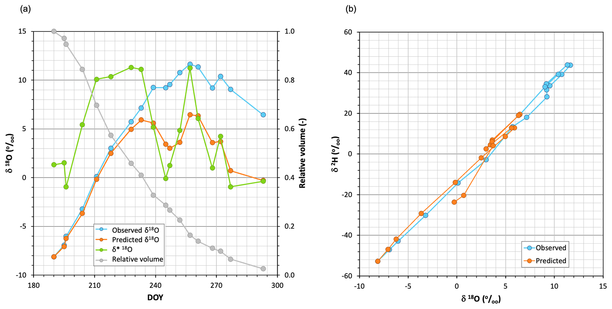
Figure 2 (a) Time series of δ¹⁸O observed in the pan water together with (unweighted) predicted and limiting δ^*18O values when Eq. (1) was applied, using the weekly averaged air temperature and relative humidity of the period studied. The relative residual volume curve is also indicated. (b) Dual plot of the δ¹⁸O observed and predicted during the period studied.

3 Results and discussion

The blue line in Fig. 2a shows the chronicle of the isotopic composition (δ¹⁸O) of the water sampled in the pan. During the first weeks the water became rapidly enriched in ¹⁸O, but after about 2.5 months (71 d), when the relative volume of water in the pan was below 20 %, it underwent alternating periods of enrichment and depletion. At the end of the experiment, the isotopic composition of the pan water was similar to that observed 10 weeks earlier. Figure A1 shows that both light isotopes evaporated rather than condensed during the experiment, including late periods of heavy isotope depletion.

Figure 2a shows that the limiting compositions δ^* obtained with Eq. (2) using unweighted T and h conditions were higher than the compositions observed for the pan water during the first 8 weeks but were lower during the rest of the experiment. The pan water isotopic compositions were adequately predicted during the first 5–6 weeks but were clearly underestimated thereafter, when the depletion periods were exaggerated.

Figure 2b demonstrates that both the observed and simulated isotopic compositions of the pan water were located near the same LEL, regardless of whether the water became enriched or depleted.

Given the high dependence of the δ^* limiting values on air relative humidity (Fig. 3), an incorrect assessment of the effective value of h was deemed the most likely cause of its underestimation using Eq. (2) and the propagation of the error to the pan water isotopic composition using Eq. (1).

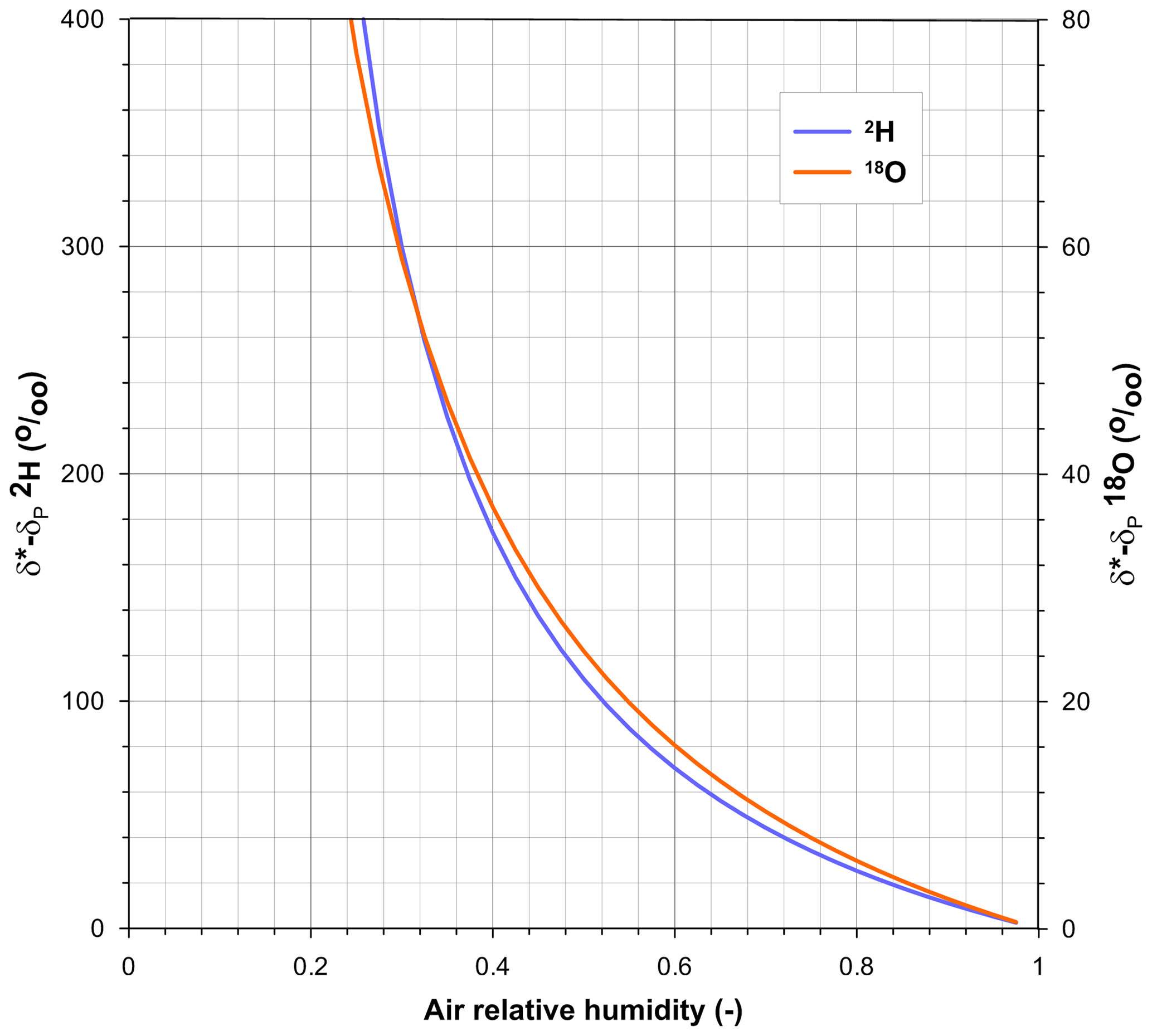
Figure 3 Relationship between air relative humidity and the differences between the limiting isotopic compositions (δ^*) and the isotopic composition of precipitation (δ_P) for ²H and ¹⁸O calculated using Eq. (2). Temperature is set at 20 ^∘C.

The difference between time-averaged and flux-weighted relative humidity is shown for 4 September, a late-summer day, in Fig. 4. For this day, the average daily h was 74 %, whereas when h was weighted with potential evaporation the mean value was 52 %. With Eq. (2) these h values correspond to δ^*18O concentrations of 5.94 ‰ and 22.15 ‰, respectively. Figures A2 and A3 show, for all the sampling dates, the differences in the daily values of T and h when obtained by either time-averaging or evaporation flux-weighting and the corresponding differences in the estimates of δ^* concentrations. Temperatures became similarly higher when flux-averaged, regardless of their magnitude. In a different way, relative humidity was habitually lower when flux-averaged but did not change when it was very high or very low.

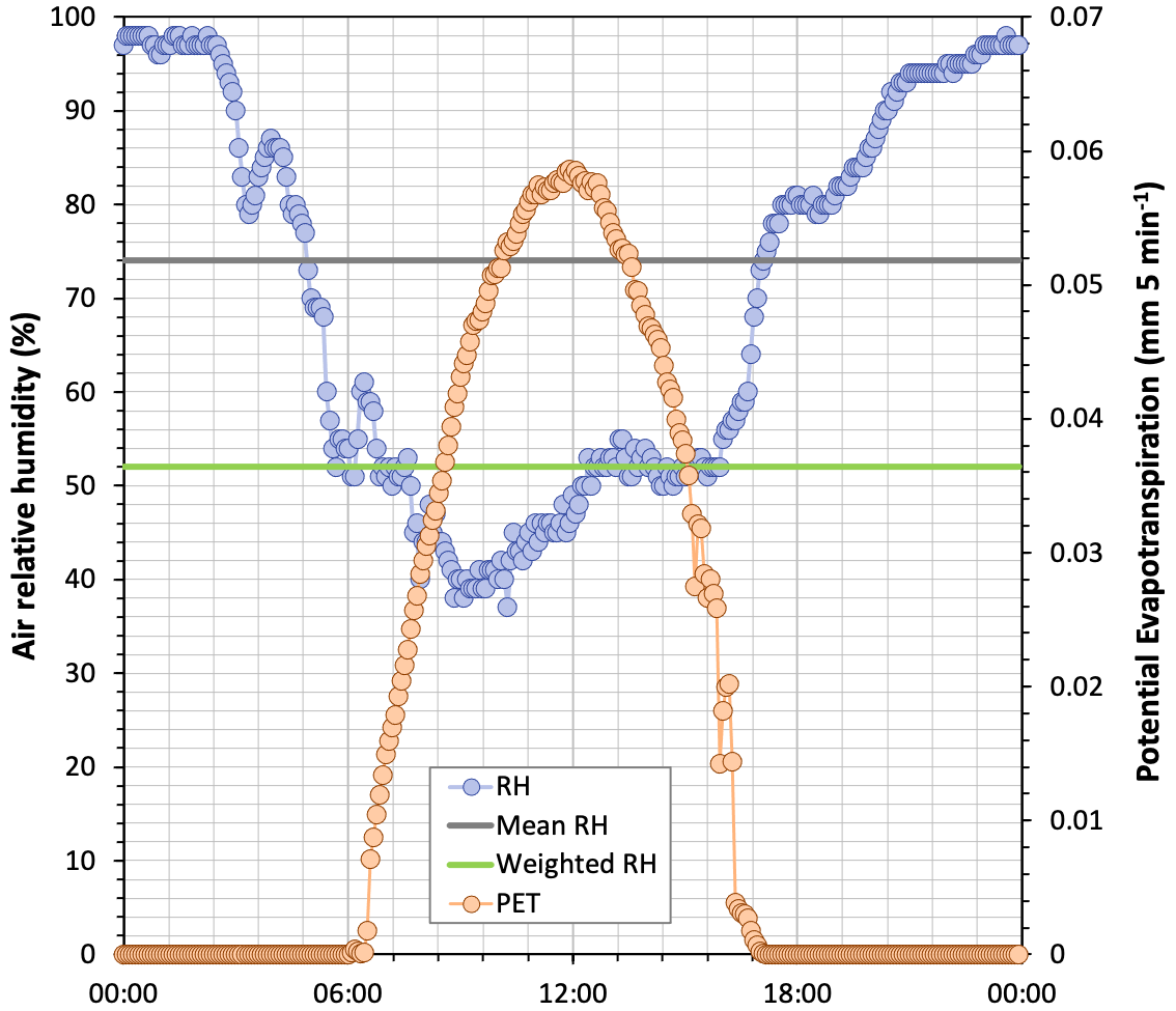
Figure 4 Time series of air relative humidity and potential evaporation for 4 September 2020 (5 min time steps). The mean relative humidity and relative humidity weighted by evaporation flux are also shown.

Subsequently, following the recommendation made by some authors (e.g. Allison and Leaney, 1982; Gibson, 2002; Gibson et al., 2008), we used T and h weighted with potential evaporation for parameterizing Eq. (1). Differences between weighted and unweighted daily values of δ^* were independent of the daily amplitudes of h (Fig. A4a) but were null when h was close to saturation and significantly increased as h decreased (Fig. A4b).

Figure 5a (chronicles) and 5b (dual plot) show the series of δ¹⁸O observed and simulated and δ^* for the studied period, showing that results clearly improved here where Eq. (1) was applied with T and h weighted, to the point of adequate simulation. Differences between unweighted and weighted δ^* values were not propagated to those of δ_L (r=0.04) due to large differences in initial δ₀ values. Figure A5 compares simulated versus observed compositions for both isotopes and parameterizations; as mentioned before, the errors associated with the unweighted T and h parameterization were evident after the eighth week. When the weighted parameterization was applied, mean absolute errors decreased by a quotient of 4, from 19.31 ‰ and 3.78 ‰ for δ²H and δ¹⁸O, respectively, to 4.88 ‰ and 0.87 ‰.

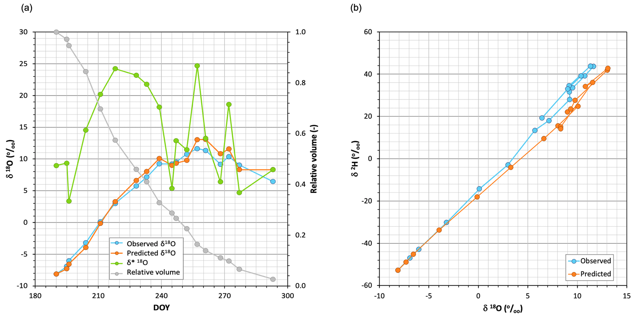
Figure 5 (a) Time series of δ¹⁸O observed in the pan water together with (weighted) simulated and limiting δ^*18O values when Eq. (1) was applied, using evaporation flux-averaged air temperature and relative humidity conditions. (b) Dual plot of the δ¹⁸O observed and predicted during the period studied.

In order to understand the environmental conditions that led to the depletion of heavy isotopes during evaporation, we analysed the dependence of the limiting δ^* values on their main drivers h and δ_A along the experiment. Figure 6 shows that, during the experiment, h ranged between 0.45 and 0.74 and δ_A between −20.5 and −13.6, whereas δ^* had a much larger range between 3.34 and 24.7. This graph demonstrates that the large variability in δ^* during the experiment shown in Fig. 4 essentially originated in the variations in h, whereas variations in δ_A had a much smaller influence (R²=0.25) that was still significant at the 5 % level (p=0.035).

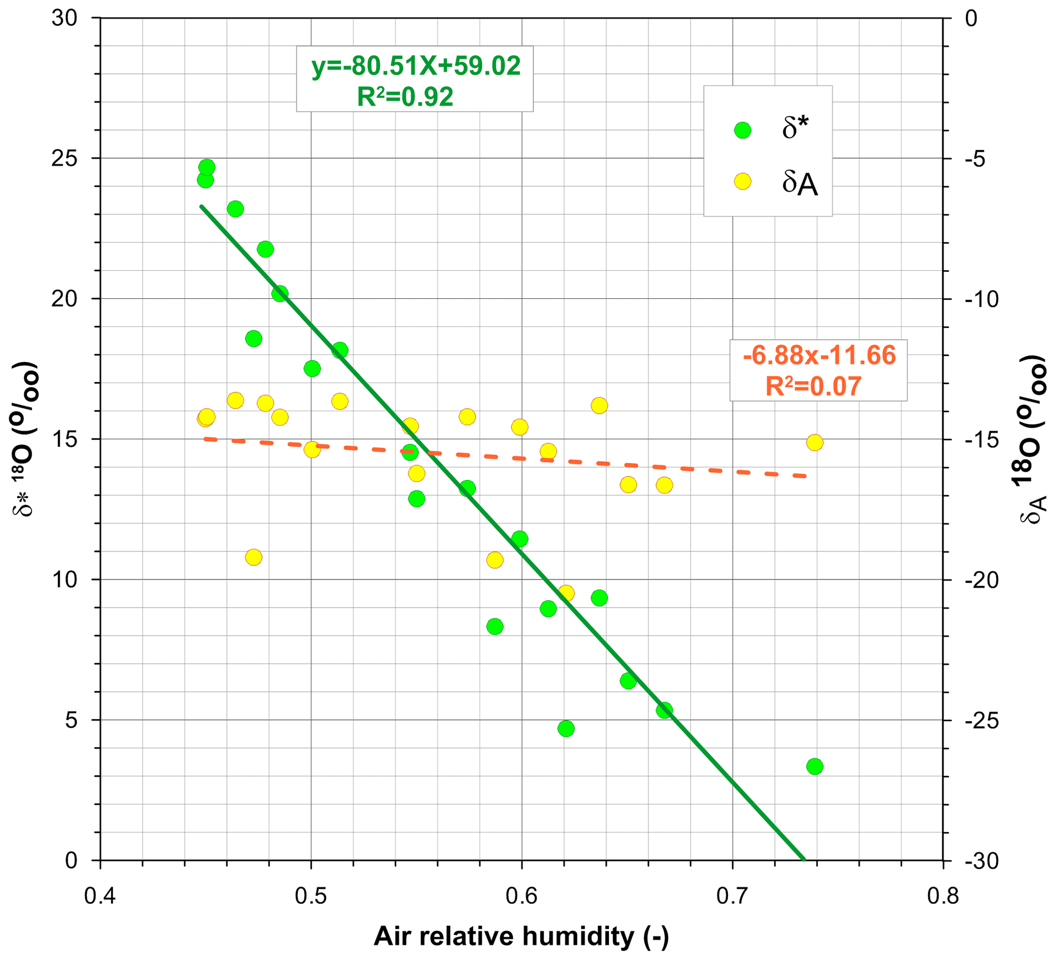
Figure 6 Weekly estimates of ¹⁸O isotopic composition, limiting (δ^*) and in air moisture (δ_A), in relation to relative humidity. Vertical scales are offset 30 ‰ from each other.

Additionally, Fig. 7, a diagram designed by Allan Rodhe to analyse the isotopic fractionation in forest throughfall (in Saxena, 1986), summarizes the role of h, δ_A, δ^*, and the isotopic composition of the pan water in the ¹⁸O enrichment and depletion events during the experiment. According to Eq. (1), evaporation will approximate the isotopic compositions of the pan water towards δ^* by enriching point values that lie below the δ^* line and depleting those above it. From bottom to top, at the beginning of the experiment, the isotopic composition of the pan water was so depleted that it became enriched in spite of high-h conditions and the lowest limiting δ^* values. After week 10, the pan water was so enriched that successive large variations in h forced alternating periods of enrichment and depletion. This analysis supports the validity of this graph for qualitatively predicting whether evaporation will determine isotope depletion or enrichment under given conditions, as proposed by Saxena (1986).

Figure 7 Evolution of the weekly differences between the isotopic composition of water and air, plotted in relation to air relative humidity (from bottom to top). The green line that connects the δ^*–δ_A points is a second-order polynomial, shown only as a visual reference.

Finally, the errors that can be committed using Eqs. (1) and (2) when parametrized with time-averaged T and h for simulating the relative volumes of water evaporated from the isotopic change are shown in Fig. 8. When time-averaged meteorological data were used, Eq. (11) predicted slightly smaller residual relative water volumes than observed for the first seven observations, but it was in mathematical error for the remaining observations. These errors are due to the fact that the limiting water isotopic composition δ^* had values between the original δ_O and the terminal δ_L ones, an impossible arrangement because, following Eq. (1), evaporation will approximate the isotopic composition of water towards δ^* by increasing or decreasing its value, but it cannot modify the isotopic composition of water by crossing the δ^* value. Figure 2a shows indeed that (unweighted) δ^* values were smaller than the observed δ values for the latter two-thirds of the experiment.

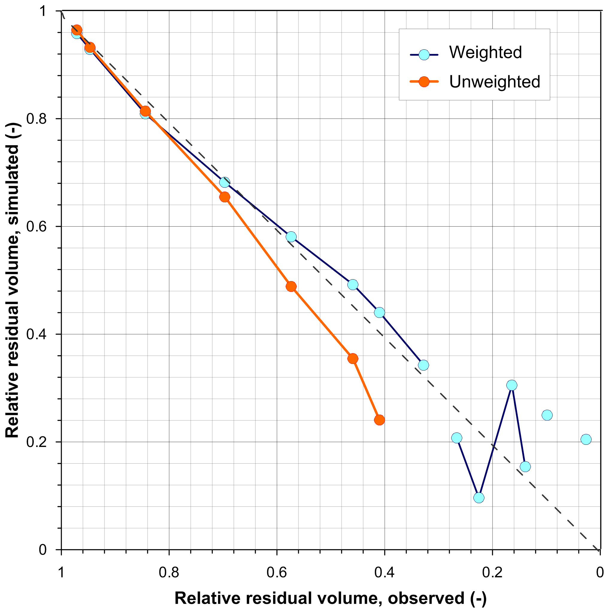
Figure 8 Simulated versus observed residual volumes of evaporating water applying Eq. (11) and comparing the use of both unweighted and PET-weighted meteorological parameters. Gaps in the lines correspond to lacking points due to mathematical errors (non-real number results) of Eq. (11).

When Eq. (11) was applied with PET-weighted meteorological data, the results were much better for most of the observations, although some mathematical errors also occurred (line discontinuities). These errors do occur because the actual δ_O of the evaporating process at every step is not the value at the start of the experiment, but the δ_L value of the former step. In Fig. 5a, these samples correspond to those that underwent ¹⁸O depletion instead of enrichment: the corresponding observed δ values were smaller than the preceding ones but larger than the corresponding limiting δ^* values, so the application of Eq. (11) yields adequate results at the weekly step scale (depletion). The analysis at the weekly step scale is not feasible when time-averaged (unweighted) meteorological data were used, because the limiting δ^* values were strongly underestimated.

In fact, Figs. 5a and 8 recall the limitations of the isotopic method for assessing the residual water volume in a pool from its isotopic composition or vice versa. This method would require a monotonic change in the pool water isotopic composition for decreasing water volume but, as already shown by Gonfiantini (1968), this requirement fails if the pool water isotopic composition approaches the limiting δ^* value due to a low residual volume associated with high relative air humidity. When this occurs, evaporation may continue with enrichment, stability, or depletion in heavy isotopes (Fig. 7).

4 Final remarks

Current knowledge establishes that water that evaporates in the open air tends to reach limiting or stationary heavy isotopic compositions (δ^*), which approach those of precipitation (δ_P) when it is in equilibrium with air humidity near saturation. In drier conditions, these δ^* values increase rapidly with decreasing air humidity and become poorly sensitive to atmospheric moisture isotopic composition.

Evaporation of water does not always induce heavy isotope enrichment but may progress without isotopic change in a steady-state process when the composition of evaporating water is equal to the limiting δ^* value. When this limiting value is exceeded, back-equilibration overwhelms the evaporative distillation and the evaporating water becomes depleted.

In this experiment, we observed several alternating weeks of heavy isotope enrichment and depletion during evaporation of pan water. These events were successfully simulated using classical equations and attributed to temporal increases in air relative humidity and corresponding decreases in the limiting δ^* values, below the composition reached by the evaporating water.

It was also possible to make qualitative graphical predictions of enrichment or depletion in heavy isotopes during periods of evaporation without the need to know the volumes of water involved.

The success of the isotopic fractionation equations needed the use of flux-weighted temperature and relative humidity conditions during the weekly periods of the experiment. When time-averaged meteorological conditions were used, the errors in the simulation of water isotopic composition were small at the beginning of the experiment when pan water was rather depleted, but they became very significant when more than half the volume of the water had evaporated; this may be attributed to both the cumulative effect of underestimated limiting compositions on the already underestimated pan water isotopic composition and more strongly propagated errors when water volumes are low.

When using the isotopic composition of evaporating waters to calculate the volume of water evaporated, the susceptibility to periods of heavy isotope depletion must be taken into account. Fortunately, when the target is to calculate the isotopic composition of the source waters, these depletion periods follow the same LEL slope as enrichment periods.

Appendix A

Some complementary figures included in this Appendix give further details on the experiment.

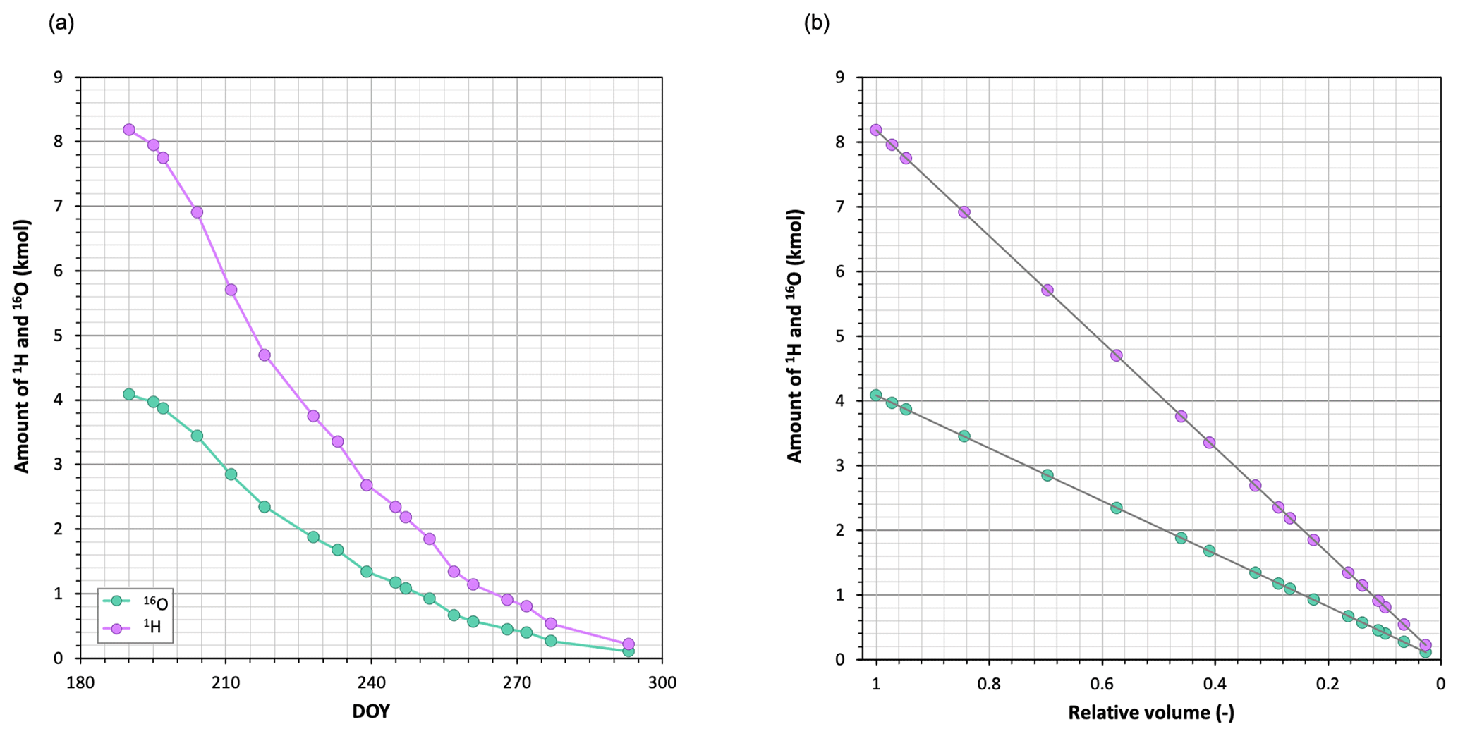
Figure A1 Quantity of light isotopes in the water during the experiment, (a) for the date and (b) for the relative residual volume and calculated using Eq. (10). Evaporation rates always exceeded condensation ones, even during the late periods of heavy isotope depletion.

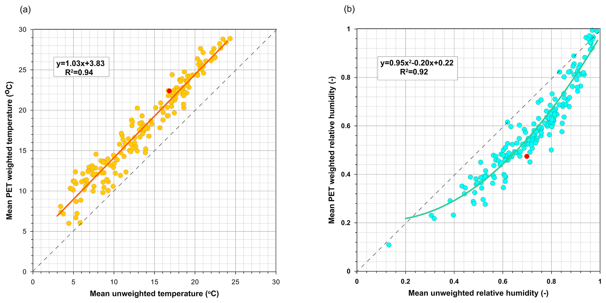
Figure A2 Comparison of the differences in daily (a) temperature and (b) relative humidity when 5 min readings were time-averaged (unweighted) or weighted with potential evapotranspiration. The red dots represent the conditions on the date shown in Fig. 5. The dashed line shows the 1:1 relationship.

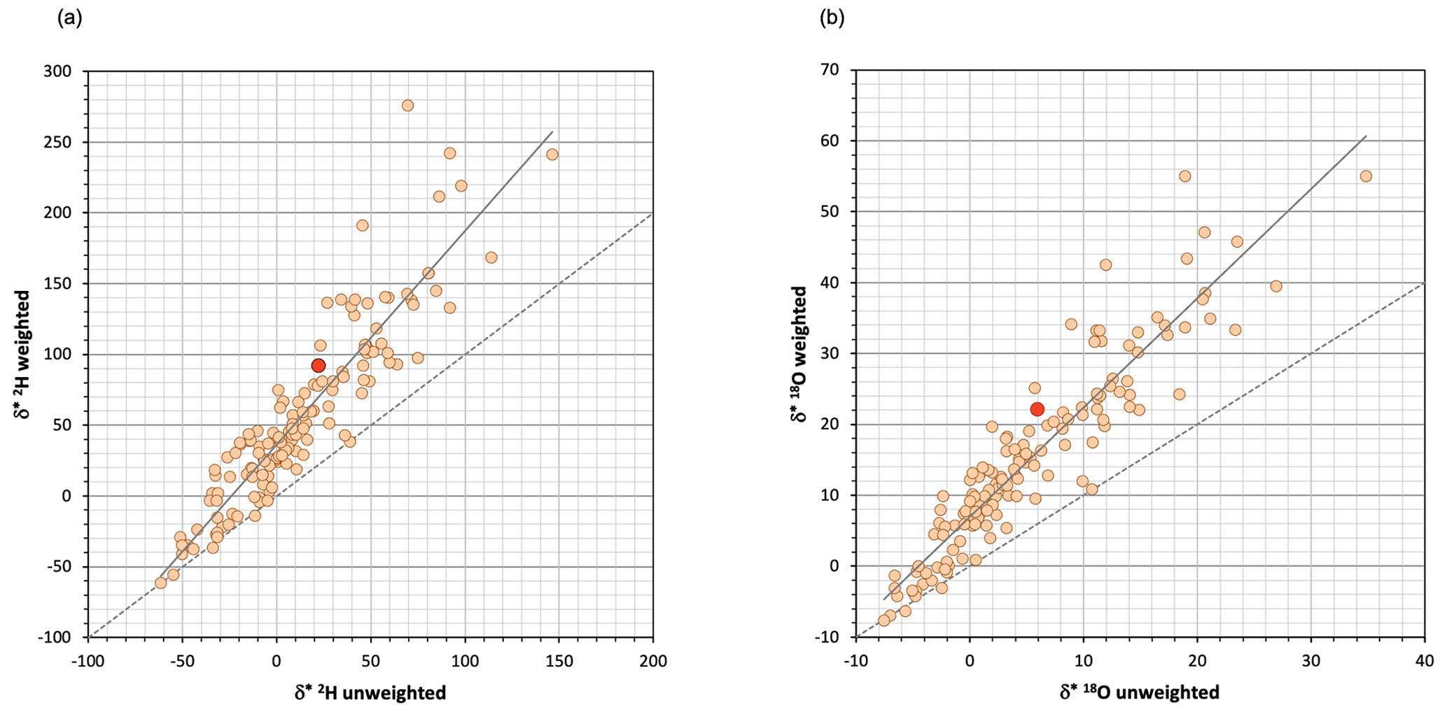
Figure A3 Comparison of the daily limiting compositions δ^* for (a) ²H and (b) ¹⁸O when 5 min readings were time-averaged (unweighted) or weighted with potential evapotranspiration. Low δ^* values show the least differences because these correspond to days with high relative humidity, as shown in Figs. 3 and A4. The red dots represent the conditions on the date shown in Fig. 5. The dashed line shows the 1:1 relationship.

Figure A4 Dependence of the differences between the daily limiting δ^* values obtained with time-averaged meteorological conditions (unweighted) and those weighted by PET (weighted) on (a) the daily amplitudes of relative humidity and (b) the weighted daily relative humidity. Equations are shown only to demonstrate the dependences.

Figure A5 Simulated versus observed heavy isotope concentrations when air temperature and relative humidity are time-averaged or weighted with potential evapotranspiration.