the Creative Commons Attribution 4.0 License.
the Creative Commons Attribution 4.0 License.
 | 30 May 2024
Leveraging multi-variable observations to reduce and quantify the output uncertainty of a global hydrological model: evaluation of three ensemble-based approaches for the Mississippi River basin
Howlader Mohammad Mehedi Hasan
Kerstin Schulze
Helena Gerdener
Lara Börger
Somayeh Shadkam
Sebastian Ackermann
Seyed-Mohammad Hosseini-Moghari
Hannes Müller Schmied
Andreas Güntner
Jürgen Kusche
Global hydrological models enhance our understanding of the Earth system and support the sustainable management of water, food and energy in a globalized world. They integrate process knowledge with a multitude of model input data (e.g., precipitation, soil properties, and the location and extent of surface waterbodies) to describe the state of the Earth. However, they do not fully utilize observations of model output variables (e.g., streamflow and water storage) to reduce and quantify model output uncertainty through processes like parameter estimation. For a pilot region, the Mississippi River basin, we assessed the suitability of three ensemble-based multi-variable approaches to amend this: Pareto-optimal calibration (POC); the generalized likelihood uncertainty estimation (GLUE); and the ensemble Kalman filter, here modified for joint calibration and data assimilation (EnCDA). The paper shows how observations of streamflow (Q) and terrestrial water storage anomaly (TWSA) can be utilized to reduce and quantify the uncertainty of model output by identifying optimal and behavioral parameter sets for individual drainage basins. The common first steps in all approaches are (1) the definition of drainage basins for which calibration parameters are uniformly adjusted (CDA units), combined with the selection of observational data; (2) the identification of potential calibration parameters and their a priori probability distributions; and (3) sensitivity analyses to select the most influential model parameters per CDA unit that will be adjusted by calibration. Data assimilation with the ensemble Kalman filter was modified, to our knowledge, for the first time for a global hydrological model to assimilate both TWSA and Q with simultaneous parameter adjustment. In the estimation of model output uncertainty, we considered the uncertainties of the Q and TWSA observations. Applying the global hydrological model WaterGAP, we found that the POC approach is best suited for identifying a single “optimal” parameter set for each CDA unit. This parameter set leads to an improved fit to the monthly time series of both Q and TWSA as compared to the standard WaterGAP variant, which is only calibrated against mean annual Q, and can be used to compute the best estimate of WaterGAP output. The GLUE approach is almost as successful as POC in increasing WaterGAP performance and also allows, with a comparable computational effort, the estimation of model output uncertainties that are due to the equifinality of parameter sets given the observation uncertainties. Our experiment reveals that the EnCDA approach performs similarly to POC and GLUE in most CDA units during the assimilation phase but is not yet competitive for calibrating global hydrological models; its potential advantages remain unrealized, likely due to its high computational burden, which severely limits the ensemble size, and the intrinsic nonlinearity in simulating Q. Partitioning the whole Mississippi River basin into five CDA units (sub-basins) instead of only one improved model performance in terms of the Nash–Sutcliffe efficiency during the calibration and validation periods. Diverse parameter sets achieved comparable fits to observations, narrowing the range for at least three parameters. Low coverage of observation uncertainty bands by GLUE-derived model output bands is attributed to model structure uncertainties, especially regarding artificial reservoir operations, the location and extent of small wetlands, and the lack of representation of rivers that may lose water to the subsurface. These uncertainties are also likely to be responsible for significant trade-offs between optimal fits to Q and TWSA. Calibration performed exclusively against TWSA in regions without Q observations may worsen the Q simulation as compared to the uncalibrated model variant. We recommend that modelers improve the realism of the output of global hydrological models by calibrating them against observations of multiple output variables, including at least Q and TWSA. Further work on improving the numerical efficiency of the EnCDA approach is necessary.
- Article
(5889 KB) - Full-text XML
-
Supplement
(2708 KB) - BibTeX
- EndNote


By quantifying water flows and storages on the Earth's continents, global hydrological models (GHMs) contribute to our understanding of the functioning of the Earth system. GHMs (including land surface models) are indispensable in the assessment of the past and future impacts of human activities on the global freshwater system in the Anthropocene, including water abstractions, dam construction and greenhouse gas emissions. In our globalized world, where local decisions affect freshwater systems worldwide, GHMs support sustainable water use by enabling the globally consistent computation of indicators of water availability and water stress.
To generate informative model outputs such a streamflow, groundwater recharge and soil water content, GHMs integrate a large amount of spatially distributed climatic and physiographic input data (including data on land cover, soil characteristics, surface waterbodies and human water use). However, they draw insufficient benefit from in situ and remote-sensing observations of model output variables to improve the quality of their output or to determine its uncertainty.
Like all hydrological models, GHMs suffer from uncertainty due to model structure, model input (in particular, climate forcing) and model parameters (Döll et al., 2016). To reduce the uncertainty of model output, models can be calibrated by adjusting the model in a way that simulated values of a model output variable optimally match observations of this variable. In basin-scale hydrological modeling, the estimation of model parameters by calibration against time series of observed streamflow is standard. This is not the case for GHMs, which is due to the limited availability of streamflow observations for many regions and the large effort required to exploit them, among other things. In global-scale hydrological modeling, model structure and input are more uncertain than in typical basin-scale modeling for large parts of the global model domain, and the density of available streamflow observations is lower. In particular, due to equifinality (Beven, 1993), uncertainty reduction by parameter estimation for GHMs is best done by utilizing observations not only of streamflow but also of other model output variables (multi-variable parameter estimation: Yassin et al., 2017; Stisen et al., 2018; Dembélé et al., 2020).
Equifinality – or its synonym, non-uniqueness – means that different combinations of model parameters (and also of model structures and inputs) may lead to a similarly good agreement between simulated and observed values of a model output variable so that it is not possible to determine an optimal (unique) parameter set (Beven, 1993). Equifinality implies that multiple model simulations, generated by, e.g., running the model with multiple parameter sets, are acceptable and informative for the model user if they (1) cannot be easily rejected as infeasible representations of the system given, in particular, the uncertainty of the observations and (2) support the specific modeling purpose, e.g., to project either low flows or floods (Beven and Smith, 2015). The ensemble of such model runs or parameter sets is referred to as “behavioral” (Beven and Binley, 1992). The concept of behavioral parameters can be applied to quantify the uncertainty of the model output that stems from the uncertainty of the observations of model output variables. However, methodological knowledge on how to best reduce and quantify model output uncertainty by multi-variable parameter estimation is lacking, in particular in global-scale hydrological modeling.
To do a multi-variable parameter estimation and related uncertainty quantification with GHMs, observations of both streamflow (Q) and terrestrial water storage anomaly (TWSA) should be used. TWSA from GRACE (The Gravity Recovery and Climate Experiment) has offered spatially uninterrupted global coverage and almost continuous monthly time series since 2003. TWSA observations integrate over all water storage compartments on the continents (glacier, snow, soil, groundwater and surface waterbodies) and thus also depend on all water flows on the continents. This is similar to Q, which is the integrative result of upstream flow and storage processes. Thus, TWSA observations complement Q observations. The coarse spatial resolution of TWSA observations of about 100 000 km2 (Vishwakarma et al., 2021) is less problematic for GHMs than for basin-scale hydrological models.
Currently, most GHMs do not use observed Q (or any other observations) to estimate parameters in the upstream basin, i.e., GHMs are not calibrated in a basin-specific manner (Bierkens, 2015). One exception is the GHM WaterGAP (Alcamo et al., 2003; Döll et al., 2003), which is calibrated in a simple manner by adjusting one to three parameters in each of the 1319 large drainage basins (Müller Schmied et al., 2014, 2021) such that simulated long-term average annual Q is close to observations. For the standard version of WaterGAP, adjustment of a larger set of model parameters is currently not done due to the equifinality problem and computational simplicity. While this limited calibration leads to a reduction in the Q bias and thus more realistic estimates of renewable water resources as compared to the uncalibrated version (and the results of other GHMs that are not calibrated in a basin-specific manner), it does not significantly improve the simulated seasonality and interannual variability of Q (Hunger and Döll, 2008). Discrepancies compared with time series of observed monthly Q (Müller Schmied et al., 2014) or TWSA (Döll et al., 2014; Scanlon et al., 2019) can be high even after the standard WaterGAP calibration. It is therefore desirable to adjust parameters that affect the seasonality of simulated Q or TWSA, as well as their interannual variability and potential trends.
Multi-variable parameter estimation can be done by various ensemble-based approaches such as (1) Pareto-optimal calibration (POC) using an optimization algorithm (Werth and Güntner, 2010); (2) the generalized likelihood uncertainty estimation (GLUE) approach for identifying behavioral parameter sets (Beven and Binley, 1992); and (3) data assimilation with the ensemble Kalman filter, in which model states and parameters are jointly updated, as suggested in Eicker et al. (2014) (hereafter, we refer to this as EnCDA). With each of these approaches, an ensemble of parameter sets is generated. While parameter estimation using an optimization algorithm (POC) is expected to be more efficient in finding (Pareto-) optimal parameter sets than a GLUE approach using a random sampling of the parameter space (Blasone et al., 2008), the GLUE approach is required to determine behavioral parameter sets that enable a quantification of the model output uncertainty given the observation uncertainty. With EnCDA, we explore here, for the first time, whether the ensemble Kalman Filter approach, which is well established for data assimilation (adjustment of model states), can also estimate model parameters simultaneously when Q and TWSA observations are assimilated.
Werth and Güntner (2010) developed a multi-variable POC scheme for WaterGAP and applied it to adjust six to eight parameters homogeneously in 28 large river basins (e.g., the Amazon, Mississippi and Lena) using both Q and TWSA observations. A similar approach was applied by Xie et al. (2012) to calibrate the SWAT model for 10 large basins in sub-Sahara Africa using observed TWSA time series and monthly mean Q values. The GLUE approach has not yet been applied with WaterGAP or other GHMs. The first successful EnCDA efforts to assimilate GRACE TWSA into WaterGAP while simultaneously estimating model parameters were made for the Mississippi River basin in the US and the Murray–Darling Basin in Australia by Eicker et al. (2014) and Schumacher et al. (2016a, b, 2018). While EnCDA with more than one observation variable (Q and remotely sensed soil moisture) has already been applied in large-scale hydrological modeling of the upper Danube basin (Wanders et al., 2014), joint EnCDA of Q and TWSA has not yet been reported. In summary, while the EnKF has been modified for parameter estimation in hydrology models in the past, no such efforts have been undertaken when assimilating both Q and TWSA observations.
The objective of this paper is to analyze how the uncertainty of the output of GHMs can be reduced and quantified by parameter estimation that utilizes observations of multiple output variables and their uncertainties. For the example of the Mississippi River basin (MRB), the paper shows how Q and TWSA observations can be utilized to obtain one optimal parameter set (the “compromise solution”), as well as ensembles of Pareto-optimal and behavioral parameter sets for the GHM WaterGAP, by evaluating the applicability of the multi-variable calibration approaches POC and GLUE and of the newly modified ensemble Kalman filter (EnCDA). It presents a method for defining performance thresholds for behavioral parameter sets based on observations and their uncertainties, as well as the initial GLUE ensemble. It should be cautioned that “performance” in this paper is mainly defined in terms of the Nash–Sutcliffe efficiency (NSE) metrics, following the custom in the hydrological modeling community, which is different from the RMSE metric, which is routinely optimized in the data assimilation community. In each approach, model parameters of all grid cells within so-called calibration data assimilation (CDA) units, either the whole MRB or five sub-basin CDAs, were uniformly adjusted. We derive conclusions for multi-variable parameter estimation and quantification of model output uncertainty in global-scale hydrological modeling, answering the following research questions:
-
What are the advantages and disadvantages of the three approaches? Is the ensemble Kalman filter, which aims at state estimation in the first place, able to compete with the dedicated model calibration approaches despite its very different ensemble generation and objective functions?
-
What is the added value of the multi-variable parameter estimation as compared to the standard WaterGAP calibration for identifying one optimal parameter set?
-
How and to what extent can WaterGAP model output uncertainty be quantified?
-
How large are the trade-offs between the optimal simulation of Q and TWSA? To what extent is Q simulation improved by calibration against TWSA only?
-
What is the added value of individually calibrating sub-basin CDAs instead of one basin CDA?
-
What are the characteristics of the optimal and behavioral parameter sets?
The paper is structured as follows. Section 2 describes the three approaches. Section 3 provides a short description of the GHM WaterGAP and explains the setup of the study, including the selection of the parameters by an initial sensitivity analysis. In Sect. 4, we present the results of our study. In Sect. 5, we discuss the research questions, and we draw conclusions in Sect. 6.
While model calibration can encompass adjustments of model structure, initial conditions, input variables and parameters, model calibration in hydrology focuses on the identification of optimal or suitable parameter sets. The focus on parameter adjustment in hydrological modeling is justified by the necessity of using many parameters that cannot be measured independently or derived from first principles. Water flows in the hydrology domain are largely dominated by the local geometry and local boundary resistances of the individual flow pathways, which is different from the water flows in the meteorology and oceanography domains (Beven, 2002). In hydrological models, water flows are expressed as a function of water storage or potential gradients, as well as of parameters that represent the highly uncertain average effects of local geometries and boundary resistances. In comprehensive hydrological models that distinguish various compartments, about 10–50 model parameters result per spatial unit. In the case of distributed models in which the spatial heterogeneity of land and water is accounted for by distinguishing a large number of spatial units such as sub-basins or grid cells, each computational unit is described by its parameters set, leading to a very large number of model parameters. GHMs covering the whole land area of the globe typically represent spatial heterogeneity on the continents by distinguishing more than 60 000 0.5° grid cells, with more than 1 million model parameters whose values need to be set to enable computation.
In the GLUE approach, an ensemble of behavioral parameter sets is derived, each of which leads to an acceptable model performance given uncertainties and model purpose; the ensemble is, in most studies, defined by model simulations exceeding certain performance thresholds. In the POC approach, an ensemble of Pareto-optimal parameter sets is generated; this ensemble does not take into account model or observation uncertainties but does consider the trade-off that occurs between the fit to various performance metrics. A parameter set is called Pareto-optimal or non-dominated if it results in a better simulation performance than any other Pareto parameter set for at least one of the objectives; none of the objective functions can be further improved without degradation of some of the other objective functions (Khu and Madsen, 2005; Werth and Güntner, 2010). In EnCDA, model parameters must be integrated into the state vector. An initial ensemble of parameter sets is then updated at each intake of observations next to the model states, and parameters ideally converge with increasing intake of observations; there is a single objective function, in which multiple objectives are implicitly weighted by considering model and observation uncertainties as given.
It is computationally challenging to work with an ensemble of parameter sets, e.g., in the context of climate impact studies or seasonal forecasting. Therefore, we also identified (pseudo-) optimal parameter sets for each CDA unit. In this section, the three multi-variable calibration approaches POC, GLUE and EnCDA are described, while a comparison between them can be found in Appendix A.
2.1 POC
POC aims to identify Pareto-optimal parameter sets. While the ensemble of Pareto-optimal parameter sets determined by POC is optimal only under the assumption that there are no observation, input and model structure uncertainties, they take into account the fact that there is rarely a parameter set that leads to a simulation of different output variable that is equally optimal with respect to all observational variables. POC as applied in this study implements an optimization algorithm such as the Borg multi-objective evolutionary search algorithm (Hadka and Reed, 2013). Based on an initial small ensemble of parameter sets derived from a priori parameter distributions, the parameter sets are updated according to the value of the objective functions (performance metrics) to achieve improved performance. Then, the model is re-run; based on the new values of the objective function, parameter sets are updated again in an iterative fashion for a pre-selected number of iterations and, thus, model runs to identify Pareto-optimal parameter sets. Due to model, input and observation errors, it is unlikely that any parameter set will lead to the highest values of all objective functions. Without additional subjective preference information on what objective function is most important, all Pareto-optimal parameter sets are considered to be equally good. From the often large number of Pareto-optimal parameter sets, a “preferred” set can be selected using a variety of approaches (Khu and Madsen, 2005). The so-called “compromise parameter set” leads to values of the applied objective functions (OFs) (or performance metrics) such that the overall performance deficit Dp regarding all OFs is minimized (Yu, 1973). Dp is the distance between the utopia point, where all OF values are at their optimal values OF*, and the OF values of the Pareto-optimal parameter sets x. According to Yu (1973),
where n is the number of objective functions, and p is a parameter that is larger than or equal to 1 and that needs to be selected. By minimizing Dp with p=2, the Euclidean distance is selected to determine the compromise parameter set.
2.2 GLUE
In the GLUE approach, a large number of different model parameter sets are generated first based on assumed a priori distributions of parameter values. In the next step, a subset of so-called behavioral parameter sets is identified from this initial set. This is done by running the model alternatively with each parameter set and then computing the values of a model performance metric using observations of model output variables, which is called the likelihood measure in GLUE (Beven and Binley, 2014). In the next step, a threshold for the performance metric is identified, below which model performance is so low that these parameter sets are considered to have a likelihood of zero. Likelihood measures and thresholds for behavioral parameter sets are subjectively selected based on the expertise of the modeler and should take into account the uncertainty of model structure, climate forcing and observations, as well as the specific modeling purpose.
Multiple observation variables can be combined for determining behavioral parameter sets by selecting the subset of parameter sets for which all performance metrics are better than their different thresholds. The selection of the metric-specific thresholds implies a type of weighting between fits to the different variables. As a subset of all behavioral parameter sets, Pareto-optimal parameter sets can be identified; the pseudo-optimal parameter set can be determined using Eq. (1). Furthermore, the likelihood of each behavioral parameter set can be derived from the performance metric such that a probability distribution of model output can be quantified.
2.3 EnCDA
In the EnCDA approach that we propose here, parameter sets of each CDA unit are optimized together with water storages in the various storage compartments and grid cells (i.e., the model states) by data assimilation with the ensemble Kalman filter (EnKF; Evensen, 1994). To this end, next to the water storages, as in all earlier EnKF implementations, we add the model parameters to the state vector. The basic idea of data assimilation with the Kalman filter approach is to optimally combine observations with simulation results at the time of the observations according to estimates of model and observation errors (Clark et al., 2008). In EnCDA, an ensemble of model runs with different parameter sets and perturbed climate inputs serves to estimate the model error, which is different from POC and GLUE. EnCDA aims to minimize a weighted RMSE; the higher the ratio of model error to observation error is, the more weight is given to the observations and the larger the adjustment of water storages and model parameters is. Water volumes and parameters, all of which are state variables, are updated in each ensemble member whenever observations are available (e.g., once per month). State update depends on the information contained in the covariance matrices of simulated states (water storages and parameters), simulated Q and observations. Covariance matrices of states and simulated Q are derived from differences between the estimates of each ensemble member and the ensemble mean. The ensemble mean of all updated water storages and Q is assumed to be the best estimator (Evensen, 2003) in the case of linear models, which is certainly not true for the simulation of streamflow, and a bias might thus be expected. In the case of models with many grid cells and various storage compartments (10 in WaterGAP), the number of updated states strongly exceeds the number of observations. To achieve plausible and stable EnCDA results regarding parameters and model output variables in complex distributed hydrological models in which the number of states exceeds by far the number of observations, the degrees of freedom may have to be reduced, and rapid changes in parameters from one time step to the next need to be avoided (Xie and Zhang, 2013). Schumacher et al. (2018) found that EnCDA with only TWSA observations is limited in constraining individual model parameters, even if the number of calibration parameters is very small, as the calibration or data assimilation system is highly underdetermined. This is why adding Q observations is promising.
The output of EnCDA regarding parameters can be viewed as a time series of recursive estimates for the parameter sets for each ensemble member, even if these parameters are modeled as stationary in time (as in this study). Here, we test the hypothesis that the parameter sets of each ensemble member at the end of the calibration/data assimilation (CDA) period can be further used, without a smoother step, to generate ensemble predictions during the validation period (in which no further assimilation is done) that fit better to observations than predictions with parameters that have not been altered by the data assimilation. The study of Eicker et al. (2014), in which only TWSA was assimilated, showed that, by applying such an approach, the ensemble means of model output values during the validation period fit better to observations of Q and TWSA than uncalibrated model output.
3.1 The global water resources and use of model WaterGAP
In this study, we applied WaterGAP 2.2d, which is comprehensively described in Müller Schmied et al. (2021). With a spatial resolution of 0.5° latitude by 0.5° longitude (55 km × 55 km at the Equator), WaterGAP computes both water resources, i.e., water flows and storages, and human water use for all land areas of the globe, except Antarctica. Water withdrawals and consumptive water use in the sectors of households, manufacturing, cooling of thermal power plants, livestock and irrigation are computed by five water use models. From the output of the water use models, the linking model GWSWUSE computes potential net water abstractions from groundwater (NAg) and surface water (NAs) as the difference between all withdrawals from and all return flows to groundwater and surface water, respectively. Time series of monthly NAg and NAs are inputs of the WaterGAP Global Hydrology Model (WGHM), together with time series of daily climate variables (Müller Schmied et al., 2021). WGHM computes various water flows (e.g., evapotranspiration, groundwater recharge and Q) and water storage variations in 10 compartments: canopy, snow, soil, groundwater and the surface waterbodies of local and global wetlands, local and global lakes, global artificial reservoirs, and rivers (boxes in Fig. 1). The term “local” means that the surface waterbodies are fed only by the runoff produced in the same 0.5° cell, while “global” wetlands, lakes and reservoirs are also fed by inflows from the upstream cells. The runoff generated in a cell from the “vertical” water balance (Fig. 1) is transported through the groundwater and, if existing, through the various types of surface waterbodies before reaching the river. Outflow from the river compartment is Q. Glaciers are not simulated in this WaterGAP version; while there are some glaciers in the most upstream parts of the Arkansas and Missouri river basins, these are not expected to strongly impact the mean TWSA of the large CDA units or the streamflow at the outlet of the CDA units (Fig. 2). To calculate TWSA time series, the sum of all 10 compartmental water storages is computed and normalized by its mean value over a reference period.
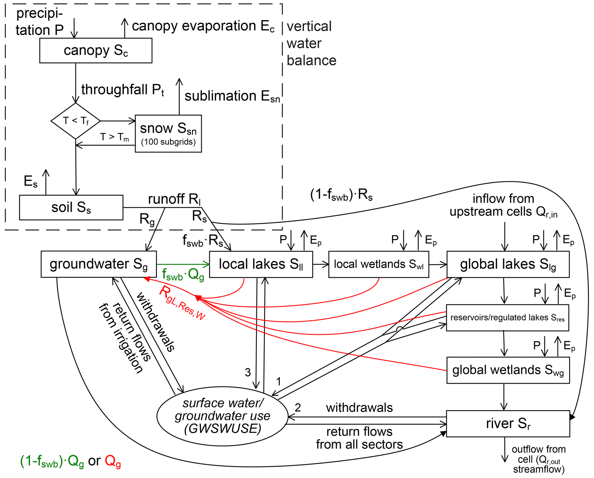
Figure 1Schematic of WGHM in WaterGAP2.2d. For each 0.5° grid cell, daily water balances of a maximum of 10 water storage compartments (boxes) are computed from their respective inflows and outflows (arrows) (Fig. 2 of Müller Schmied et al., 2021). Green and red colors indicate processes that occur only in grid cells with humid and (semi-) arid climate, respectively. Es: soil evapotranspiration, Ep: potential evapotranspiration, Rg: groundwater recharge from soil, Rs: fast surface runoff and subsurface runoff, : groundwater recharge from surface waterbodies, Qg: groundwater discharge to surface waterbodies and the river, Fswb: area fraction of surface waterbodies. Net groundwater abstracts are taken from the groundwater storage compartment, while net surface water abstractions are taken from global lakes or reservoirs in the cell (priority 1), the river (priority 2) or local lakes (priority 3).
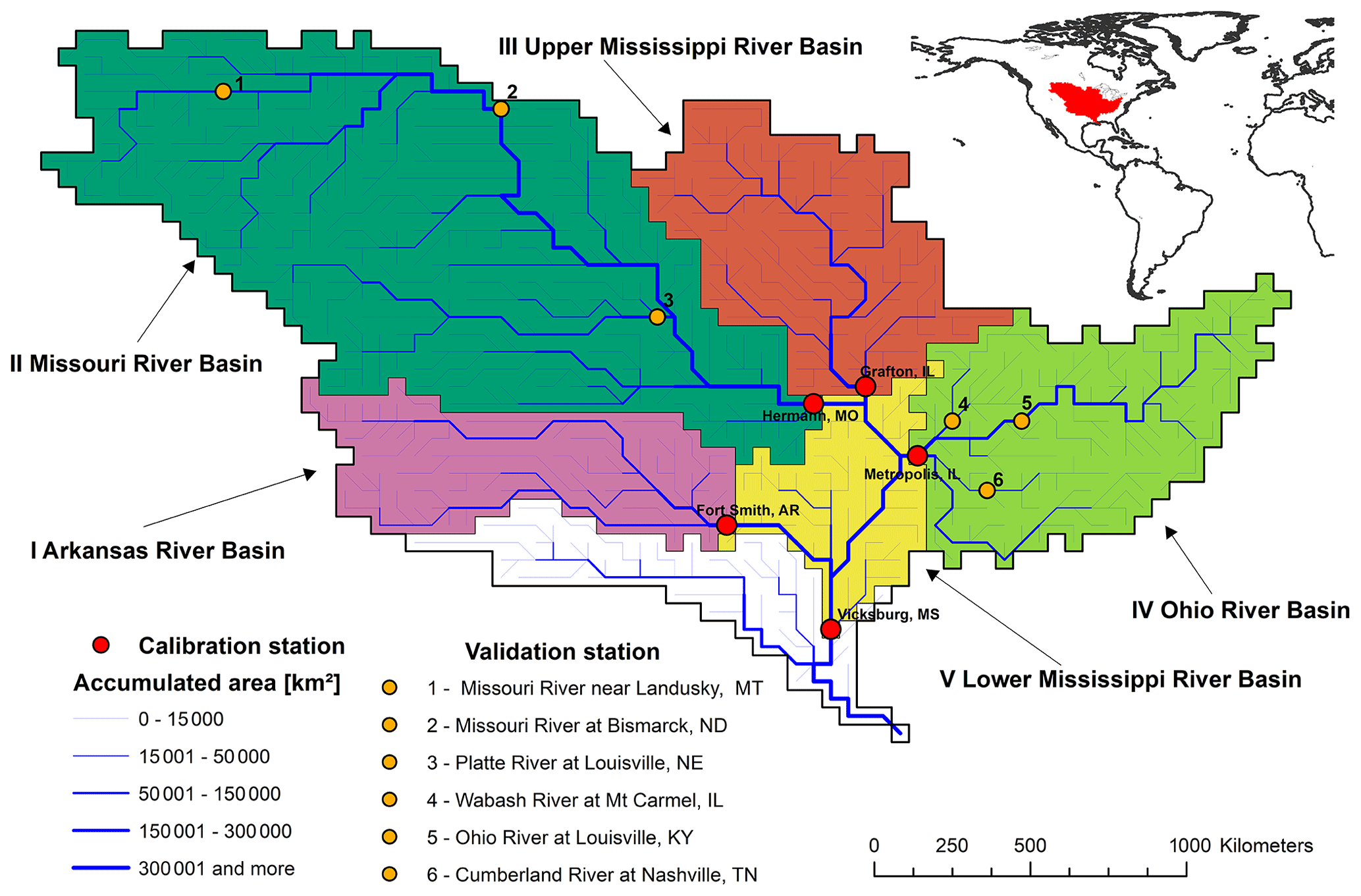
Figure 2The Mississippi River basin as represented by the 0.5° × 0.5° grid cells in WaterGAP, with delineation of the five CDA units. The CDA units were defined as the upstream cells of the five indicated calibration stations (streamflow gauging stations, shown in red). The stream network implemented in WaterGAP is shown, indicating the upstream areas of each grid cell by the line width. In addition, the locations of the six streamflow validation stations are plotted, shown in orange.
In the ordinary differential equations describing the dynamics of the individual water storage compartment, outflows are parameterized as a function of compartmental water storage (Müller Schmied et al., 2021). Other important model parameters determine the maximum values of compartmental water storage, such as the maximum soil water storage in the effective rooting zone (soil compartment) or the active lake depth, which defines the maximum height of the water table of local and global lakes above the outflow level. Parameters affecting potential evapotranspiration govern the simulated atmospheric demand for water. Temperature-related parameters are important for snow processes.
As a standard, WGHM is calibrated against observed mean annual Q by adjusting one model parameter, the runoff coefficient, and, if necessary, two correction factors (Müller Schmied et al., 2021). In the equation that describes the soil water dynamics, the runoff coefficient determines, together with soil water saturation, the amount of runoff from the land RL; it varies between 0.1 and 5. The larger the runoff coefficient is, the smaller the runoff becomes. If the adjustment of the runoff coefficient is not sufficient to not exceed a maximum discrepancy between simulated and observed mean annual Q of 10 %, a multiplicative areal correction factor for runoff from land is introduced that also corrects evapotranspiration (range of 0.5 to 1.5). If this is still not sufficient to match observed Q within 10 %, the Q in the grid cell where the gauging station is located is multiplied by a station correction factor. This violates the mass balance but is done to avoid error propagation to the downstream basins. In the standard WaterGAP, the calibration period was 1980–2009 if stream data were available for the station; otherwise, it was the most recent earlier period. The runoff coefficient in basins without Q observations is determined by a regression approach, where calibrated runoff coefficients are related to various characteristics of the drainage basins (Müller Schmied et al., 2021). With this calibration and regionalization approach, a median Nash–Sutcliffe efficiency of 0.52 and a median Kling–Gupta efficiency of 0.61 are achieved for the fit of the time series of monthly Q at the 1319 calibration stations. The median correlation coefficient of 0.79 indicates an often poor simulation of the timing of monthly Q both seasonally and interannually. WaterGAP 2.2d tends to underestimate the variability of monthly Q in northern snow-dominated river basins (Müller Schmied et al., 2021). It underestimates the mean annual TWSA amplitude in 66% of the 143 investigated river basins by more than 10 %. TWSA trends – in particular, positive trends – are often underestimated (Müller Schmied et al., 2021; Scanlon et al., 2018).
3.2 Calibration setup for the Mississippi River basin
3.2.1 Study period and CDA units
Due to TWSA and climate input data availability, the study period was limited to January 2003 to December 2016. The study area excludes the most downstream part of the Mississippi River basin (MRB) due to a lack of Q observations. The Q gauging station at Vicksburg in the lower MRB is the most downstream station with a long-term record (Fig. 2). Hereafter, we refer to the upstream area of Vicksburg as the whole MRB. We study two variants of the spatial configuration of CDA units, in which calibrated parameters were uniformly adjusted. Either the whole MRB is treated as one CDA unit or the MRB is subdivided into five CDA units. In the latter variant, four of the five CDA units (Arkansas River basin, Missouri River basin, upper MRB and Ohio River basin) are upstream river basins that are defined as the drainage basin of four gauging stations for which data for the study period 2003–2016 are available (Fig. 2). The fifth CDA unit is the lower MRB, which receives inflow from the four upstream CDA units. We divided our study period into a calibration period for parameter estimation from 2003 to 2012 and a validation period, in which the model is run with the estimated parameters, from 2013 to 2016. Q is additionally validated at six gauging stations that were not used for calibration (Fig. 2).
3.2.2 Observational data
Q data were obtained from the Global Runoff Data Centre (https://www.bafg.de/GRDC/, last access: 31 May 2019) and the US Geological Survey (https://maps.waterdata.usgs.gov/mapper/, last access: 15 July 2019). For monthly Q observations, a random error of 10 % is assumed based on the review of McMillan et al. (2012) and the study of Westerberg et al. (2016) for the UK; the latter determined a median error for the mean flow of 12 %. Actual percent errors are extremely variable depending on temporal aggregation, the Q value itself and various local conditions (Di Baldassarre and Montanari, 2009). In the EnCDA approach, an additional error of 10 % of the temporal average of the Q observation time series was applied as this led to more stable EnCDA results.
To obtain TWSA observations for this study, level-2 GRACE data (spherical harmonic coefficients, SHCs) from TU Graz (ITSG Grace2018; Mayer-Gürr et al., 2018) were evaluated over the CDA units. These data represent the Earth's time-variable gravity field as observed by the GRACE satellites via K-band ranging (KBR) and GNSS tracking. We derived TWSA from SHCs up to degree and order 96, applying the DDK3 filter (Kusche et al., 2009) and corrections for low-degree terms and effects, such as glacial isostatic adjustment, following Gerdener et al. (2020). As the temporal mean value of GRACE-derived terrestrial water storage is unknown, it is a widely followed approach to normalize the monthly TWSA values relative to a constant mean over a certain reference period, here taken to be from 2003 to 2012. Uncertainties (1σ errors) were propagated to TWSA maps based on the full variance–covariance matrix of the TU Graz data; this accounts for orbital effects and the generally meridional behavior of errors. To investigate the influence of different level-2 GRACE products, we compared the unit-averaged TWSA time series from ITSG-Grace2018 with TWSA derived from the Release-06 version of the Center for Space Research (CSR) and the Geoforschungszentrum (GFZ). For the whole MRB, 42 % of the CSR and 35 % of the GFZ monthly values were found to be within 1 standard deviation of the TU Graz solution, and 76 % of the CSR and 61 % of the GFZ monthly values were within 2 standard deviations of the TU Graz solution. Unexpectedly, the values are even higher for all sub-basin CDA units. Therefore, we decided to use ±2 standard deviations of the propagated GRACE uncertainties for quantifying the TWSA observation error in this study. Information on the uncertainty of GRACE TWSA data is provided in Sect. S1 in the Supplement.
3.2.3 Climate forcing
Climate forcing required for both the irrigation water use model and WGHM encompasses time series of daily near-surface air temperature, total precipitation, downward shortwave radiation and downward longwave radiation. In this study, we applied the 0.5° GPCC-WFDEI data set, where ERA-Interim reanalysis data of ECMWF have been bias-corrected by monthly precipitation time series of the Global Precipitation Climatology Centre and by other observations (Weedon et al., 2014). Monthly precipitation was corrected for wind-induced undercatch (Weedon et al., 2014).
3.2.4 Calibration parameters
Experience suggests that no more than five to six parameters can be estimated for each calibration objective (Efstratiadis and Koutsoyiannis, 2010). Many parameters in WaterGAP are spatially distributed, such as the parameter maximum soil water storage in the effective root zone Smax, which is computed as the product of soil water storage between field capacity and wilting point from a data set that provides a different value for each 0.5° cell and a rooting depth that is a fixed assigned value for each class of land cover, with one dominant land cover per cell. Other parameters are set globally to the same value, e.g., the groundwater discharge coefficient. To enable an adjustment of the cell-specific value of a distributed parameter like Smax, one may choose to either adjust the land-cover-specific rooting depth in each CDA unit or introduce a multiplier of cell-specific Smax as a calibration parameter. As the number of free (calibration) parameters should be limited given limited observations and equifinality, the second approach was chosen. For all spatially distributed parameters, multipliers were introduced that serve as calibration parameters, while globally uniform parameters are directly calibrated.
In Table 1, information about the 24 potential calibration parameters that were investigated in this study is provided, including their estimated a priori uncertainty range. They are ordered mainly according to the water storage compartment (Fig. 1) that they immediately impact due to inclusion in the respective water balance equation. In addition, multipliers for precipitation and net radiation are included as calibration parameters, which were found to be the parameters that the TWSAs of the 33 largest river basins worldwide are most sensitive to (Schumacher et al., 2016b). The two multipliers for the net abstraction of groundwater and surface water are allowed to become negative as, e.g., an initially simulated positive net abstraction from groundwater (where water is removed from the ground due to pumping) may, in reality, be negative. The latter is the case if infiltration of irrigation water that was taken from surface water sources dominates groundwater abstractions in the grid cell. For some parameters, the selected range was influenced by previous analyses of the WaterGAP model performance. Uniform distributions were assumed for all parameters.
Table 1WGHM parameters, the range of assumed uniform a priori distributions used for sensitivity analysis and calibration, and as the CDA units in which parameters were adjusted in this study. The parameters are categorized according to the processes or water storage compartments that they directly affect. P: precipitation, EP: potential evapotranspiration, CA: canopy, SN: snow, SL: soil, GW: groundwater, SW: surface water, NA: net abstraction of water by humans.
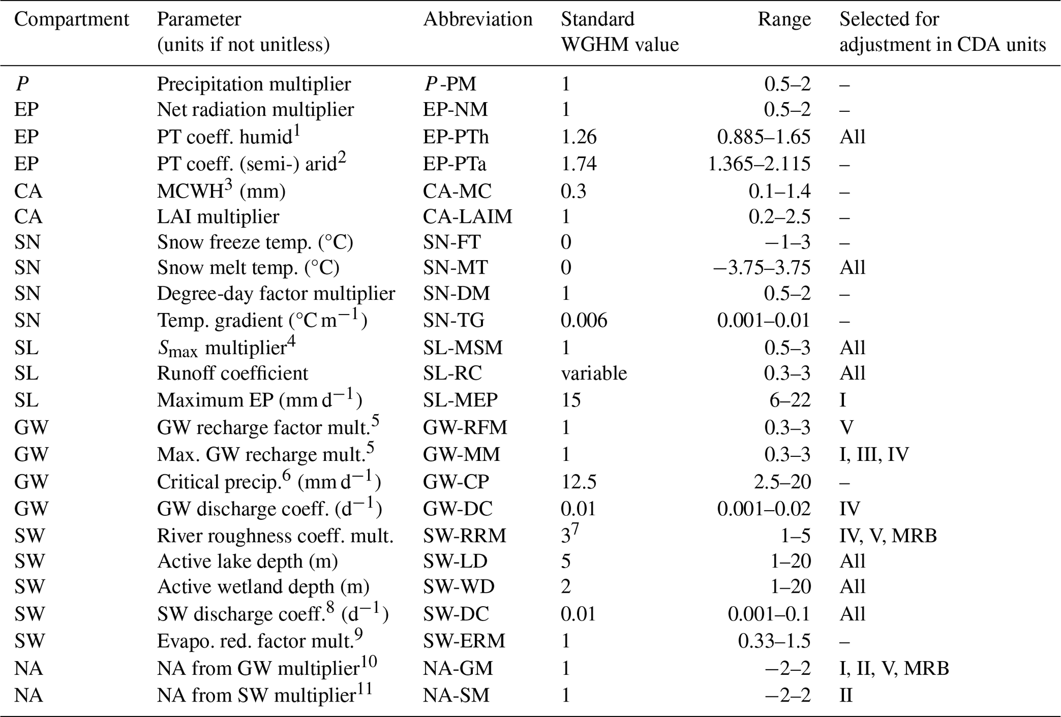
1 Priestley–Taylor coefficient in humid grid cells. 2 Priestley–Taylor coefficient in (semi-) arid grid cells. 3 Maximum water storage on canopy per leaf area index (LAI). 4 Multiplier for maximum soil water storage in the effective root zone. 5 Groundwater recharge is capped at 95 % of total runoff from land Rl. 6 In (semi-) arid grid cells, there is only GW recharge if daily precipitation exceeds the value of the parameter critical precipitation. Otherwise, the potential GW recharge remains in the soil. 7 For most river basins, including MRB. 8 For lakes and wetlands. 9 To take into account the impact of temporally varying areas of lakes, reservoirs and wetlands on evaporation. 10 Multiplier for net abstraction from groundwater. 11 Multiplier for net abstraction from surface water (reservoirs, lakes and rivers).
The Q of larger rivers in the MRB is strongly impacted by the management of the many artificial reservoirs. The water balance of large (i.e., global) reservoirs is simulated in WGHM with an algorithm that distinguishes reservoirs with the main purpose of irrigation from others; different equations are used for reservoirs with a large ratio of storage capacity to mean annual Q compared to those with a small ratio. With any globally applied algorithm, human decisions on reservoir management are very difficult to simulate, and adaptation of some parameters is not likely to lead to better simulation results unless each reservoir is dealt with individually. Therefore, no parameter of the reservoir algorithm was adjusted in this study. This limits the ability of the calibrated model to achieve a good fit to observations in river basins with many reservoirs, such as the Missouri River basin (Fig. B1a in the Appendix).
From the potential calibration parameters, a small number of calibration parameters were selected for each CDA unit by a sensitivity analysis to limit equifinality. The sensitivities of four output variables (simulated Q, TWSA, snow storage and water storage in local lakes) to all 24 parameters were analyzed separately for each of the six CDA units using the standard version of WGHM. For the sensitivity analysis, the elementary effect test (EET) method of Morris (1991) was applied, where the average of the elementary effects, i.e., the amount of change in the simulated variable due to a change in a parameter value, is used as the sensitivity measure or sensitivity index. The change in the variable is computed as the root mean square difference between a reference simulation and the simulation of the variable after deviating the parameter from its reference value. The EET method is computationally inexpensive and recommended for parameter ranking and screening (Pianosi et al., 2016). A total of 1000 random parameter sets were generated by Latin hypercube sampling and were used as the reference parameter values. Then, one at a time, each reference parameter set was perturbed for each of the 24 parameters following a radial design proposed by Campolongo et al. (2011), which resulted in a total number of 25 000 (i.e., 1000 × (1 + 24)) parameter sets. Parameters were ranked separately for each of the four output variables.
The precipitation multiplier (P-PM) and the net radiation multiplier (EP-NM) can correct biases of the climate forcing. P-PM was excluded from calibration, even though it ranked first in all six CDA units for almost all four test variables, for two main reasons. First, the precipitation input is perturbed in EnCDA, and an additional multiplier would lead to a double-counting of precipitation uncertainty. Second, mean annual precipitation in the CDA units of WaterGAP climate forcing does not differ much from the values derived from the high-resolution (4 km) PRISM data set for the USA (Table S1). Potential evapotranspiration is a function of both net radiation and the Priestley–Taylor coefficient. Even though EP-NM ranked somewhat higher in all CDA units than the Priestley–Taylor coefficient for humid areas (EP-PTh), we decided to adjust only EP-PTh (Table 1) as it is an actual model parameter and not a climate forcing correction factor (the MRB is mainly humid).
Then, we selected, for each variable, those top-ranking parameters among the remaining 22 parameters that, together, contribute at least 50 % of the combined total effect, i.e., the sum of the elementary effect for all parameters. Application of this threshold ensures that only the most influential parameters of a given variable are selected and that the total number of selected parameters remains rather small. We found that, in each of the six CDA units, the snow melt temperature (SN-MT) accounts for more than half of the total effect for the variable snow storage, and the variable local lake storage is most sensitive to the parameters of active lake depth (SW-LD) and discharge coefficient for surface waterbodies (SW-DC) (Table S2). SN-MT is also much more important than the other three snow parameters for Q and TWSA. TWSA and Q are strongly influenced by more parameters than snow and local lake storage; three to five parameters cover at least 50 % of the total effect in the case of TWSA, and this increases to four to five parameters in the case of Q. The three most influential parameters for both TWSA and Q are, in almost all CDA units, the runoff coefficient (SL-RC), the Smax multiplier (SL-MSM) and the PT coefficient for humid areas (EP-PTh). Exceptions are the downstream lower MRB (EP-PTh and SL-RC not influential for TWSA), where the inflow into the CDA unit, which is prescribed based on the POC compromise solution parameter sets, dominates streamflow, and the driest basin of Arkansas (EP-PTh is not influential for TWSA) (Table S2). For each CDA unit, 8–10 calibration parameters were selected (Table 1). As a result, all together, 47 parameters were adjusted if the five sub-basin CDA units were used for model calibration.
Seven parameters were selected as calibration parameters in all CDA units (Table 1). For each CDA unit, an additional one to three calibration parameters were selected as they had a particularly high sensitivity rank due to the specific characteristics of the CDA unit. For example, the multiplier for net abstractions from groundwater (NA-GM) was selected in four CDA units where these abstractions are high (Fig. B1d) and lead to groundwater depletion, which strongly affects TWSA. The multiplier for net abstractions from surface water (NA-SM) was only selected for the Missouri River basin, with the highest net abstractions from surface water (Fig. B1e). The maximum groundwater recharge multiplier (GW-MM), which affects the soil-texture-specific maximum amount of daily groundwater recharge, was selected in three CDA units, while the multiplier for the fraction of groundwater recharge (GW-RFM) was selected for one other CDA unit. The calibration parameter of maximum potential evapotranspiration (SL-MEP), which limits actual evapotranspiration, was found to be influential in the driest CDA unit of the Arkansas River basin. Altogether, 14 out of the 24 parameters in Table 1 were selected as calibration parameters in the study on MRB.
3.3 Performance and uncertainty metrics
In this study, we only consider performance metrics for the simulated monthly time series of Q and TWSA as they form the basis for calculating hydrological signatures, such as drought or flow indicators, that are used in global-scale water resource assessments. While the mean is an important characteristic in the case of Q, this is not true for TWSA, which is an anomaly with zero temporal mean during the reference period. The Nash–Sutcliffe efficiency is a traditional performance metric in hydrological modeling. It provides an integrated measure of model performance concerning mean values and variability and is computed as
where μobs is the mean of observations, and sim(t) and obs(t) refer to the simulated and observed values, respectively, at time step t of a total number of time steps n. The Kling–Gupta efficiency, together with its three components, enables one to distinguish model performance regarding correlation, bias and variability (Kling et al., 2012), with
where CC is the correlation coefficient, and
where σ is the standard deviation, and μ is the mean; the subscripts sim and obs refer to the simulated variate and observations of that variate, respectively. Expressing variability as the ratio of the coefficients of variation (Eq. 5a) ensures that bias and variability are not cross-correlated (Kling et al., 2012). In the case of TWSA, the bias is set to 1 in the computation of the Kling–Gupta efficiency (KGE), and
The optimal value of all the above performance metrics is 1.
The uncertainty of model output, as derived from the model output ensemble, can be quantified by two uncertainty metrics. In the case of Q, the average uncertainty bandwidth (AUBW) is expressed as a fraction of the ensemble mean (modified from Jin et al., 2010), with
where t refers to the month, and n is the total number of months. In the case of TWSA,
AUBWQ can be expressed in percent (%), while the unit of AUBWTWSA is in millimeters (mm). Here, the highest and lowest values among all ensemble members are used as upper and lower limits in each month and make up the uncertainty bounds of the simulation. The metric “coverage of observations by model output” (CO) is calculated as the percentage of monthly observations, including their uncertainty bounds (derived from observation errors described in Sect. 3.2.2), that are contained within the uncertainty bands of the model output. A large CO value and a small AUBW value indicate a low model output uncertainty.
3.4 Implementation of calibration approaches in this study
3.4.1 POC
The state-of-the-art optimization algorithm Borg MOEA (Borg multi-objective evolutionary algorithm; Hadka and Reed, 2013) was applied to search the parameter space to find Pareto-optimal parameter sets. Borg MOEA not only amalgamates search operators (i.e., algorithms to generate a new generation of solutions from their parents) and strategies from benchmark optimization algorithms like NSGA-II, ε-NSGA-II, ε-MOEA and GDE3; it also has the capability to exploit these operators based on their performance in producing better offspring for the optimization problem at hand. Apart from the auto-adaptive operator recombination strategy, Borg MOEA includes a restart mechanism upon the occurrence of a search stagnation and strategies like population resizing and adaptive archive sizing. The NSEs of monthly time series of Q and TWSA in the calibration period, NSEQ and NSETWSA, were chosen as the two objective functions. For all CDA units, the initial population size was 400, and the improvement threshold ε (i.e., the side length of the ε box) was set to 0.005 for all objectives. All other parameters of the algorithm were set to their recommended values (Hadka and Reed, 2013).
All WHGM model runs for the six CDA units started in 1991. Calibration of the five sub-basin CDA units was done sequentially as follows. First, the four upstream CDA units (Fig. 2) were calibrated independently from each other. Q and TWSA in the downstream CDA unit V, the lower MRB, depend on inflow from the four upstream CDA units. For each upstream CDA unit, the parameter set resulting in the highest NSEQ at the respective calibration station was selected to transfer the best estimate of monthly Q to the downstream CDA unit. These parameter sets were then used in the calibration of the downstream CDA unit, which required running the model for the whole MRB. Due to the high computational demand of WHGM, we restricted each calibration to a maximum of 20 000 model runs. The POC application was run in parallel using openmpi-4.0.1 on 401 nodes of a Linux cluster machine with a Scientific Linux 7 environment. The total runtime for the six CDA units was 72 h.
3.4.2 GLUE
For each of the six CDA units, a random ensemble of 20 000 parameter sets was generated by Latin hypercube sampling (Campolongo et al., 2011), only varying the 8–10 influential parameters indicated in Table 1. Then, individual WGHM model runs were performed for the MRB and the four upstream CDA units (Fig. 2). Similarly to the POC approach, all ensemble runs for the downstream CDA unit V, the lower MRB, were performed using, for each of the four upstream CDA units, the GLUE parameter sets that resulted in the highest NSEQ at the upstream calibration station. All GLUE runs started in 1991 and were done on the same Linux cluster machine as the POC runs. The total runtime for the six CDA units was 53 h, 26 % less than for POC with the same number of model runs.
Monthly time series of spatially averaged TWSA and Q at the calibration and validation stations during both the calibration and validation periods were written as output, and the performance metrics (Sect. 3.3) were computed. To identify behavioral and Pareto-optimal parameter sets, as well as the compromise parameter sets (Eq. 1), NSEQ and NSETWSA were used as likelihood measures.
To assess the impact of observation errors of Q and TWSA on model performance, the monthly time series of observed Q and TWSA were perturbed based on the observation errors described in Sect. 3.2.2. A uniform distribution of errors with a range of ±10 % was assumed for Q, and ±2 standard deviations of the computed GRACE error distribution was assumed for TWSA (see Sect. 3.2.2). A total of 1000 realizations of observations of Q and TWSA were generated. Then, NSEQ and NSETWSA values for each of the 1000 perturbed observation time series compared to each of the 20 000 WaterGAP time series were computed. Finally, the Pareto-optimal parameter sets for each of the 1000 realizations of observations were identified. This approach of taking into account the observation uncertainty for the selection of behavioral parameter sets is similar to the approach taken by Blazkova and Beven (2009).
3.4.3 EnCDA
EnCDA was performed by coupling the Parallel Data Assimilation Framework (PDAF; Nerger and Hiller, 2013), which implements an EnKF approach, to WGHM (Gerdener et al., 2023). Regarding the forcing data, an additive error of ±2 °C for the temperature (with a triangular distribution around 0) and a multiplicative error of ±10 % for the precipitation perturbation (with a triangular distribution around 1) (Eicker et al., 2014) were used. For each ensemble member, these errors were set individually for each month and grid cell and were applied to the daily forcing values. A spin-up phase run over 1991–2002 was performed to generate initial conditions for the calibration period. The EnKF is used to simultaneously update model parameters and storages during the calibration period 2003–2012 following Eicker et al. (2014), Schumacher et al. (2016a, b) and Gerdener et al. (2023) but considering Q observations in addition to GRACE TWSA. For this, the state vector is augmented by CDA unit-specific calibration parameters. To avoid the system being underdetermined, TWSAs in 4° grid cells instead of TWSA averages over the CDA units were assimilated. Calibration parameters and water storages were adjusted with monthly time steps.
In the case of the CDA unit covering the whole MRB, the EnCDA was performed by the parameters indicated in Table 1 while assimilating GRACE TWSAs in 4° grid cells over the whole basin, along with Q at the Vicksburg gauge station. For the sub-basin calibration, the EnCDA was applied separately to the four upstream CDA units first. Then, the parameter sets of each ensemble member of the four upstream CDA units were set to the values obtained for December 2012. For calibrating the downstream CDA unit V with EnCDA, the 32 parameter sets in each of the four upstream CDA units were held constant, and states in these CDA units were not updated by DA. Parameters were perturbed independently per CDA unit without generating spatial correlations as different parameters are considered for the different CDA units (Table 1). An attempt to simultaneously calibrate all five CDA units was not successful. Differently from POC and GLUE, the performance metric NSE was not used to generate the optimized parameter set ensemble but only to determine behavioral parameter sets and the compromise parameter sets, as well as for model output validation.
Only 32 ensemble members were generated due to the very high computational demand of EnCDA state estimation (as compared to POC and GLUE). It is prohibitive to generate ensemble sizes comparable to model calibration approaches (several 10 000 s) as, unlike POC and GLUE, EnCDA estimates not only model parameters but also model states.
Simulations for the validation period 2013–2016 were done by continuing the 32 model runs of the calibration period with the 32 parameter sets estimated for December 2012 without any data assimilation. The ensemble mean of the simulated output variables of the 32 ensemble runs during the validation period is assumed to be the best estimate of the time series of output variables. The EnCDA application was run in parallel using openmpi-3.1.4 on a Linux cluster machine with a Linux CentOS 7.9 environment and 70 nodes. The total runtime for the six CDA units was 72 h.
4.1 Model performance during the calibration period 2003–2012
Multi-objective parameter estimation may be aimed at determining (1) an optimal model parameter set that is identified by weighting the multiple calibration objectives, e.g., the compromise solution (Eq. 1); (2) Pareto-optimal parameter sets; or (3) an ensemble of behavioral parameter sets that lead to model output that fits reasonably well to observations given observations and other uncertainties. In any case, the calibrated parameter sets are specific to the applied model structure and input, including climate forcing, net abstractions of surface water and groundwater, and physiographic characteristics such as the existence of surface waterbodies or soil properties per grid cell.
4.1.1 Optimal parameter sets
Differences between calibration approaches
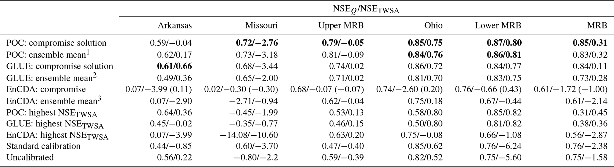
Table 2 and Fig. 3 show the performance of the (Pareto-) optimal parameter sets as measured by NSEQ and NSETWSA. As expected, the POC approach is superior to the GLUE approach in identifying Pareto-optimal parameter sets due to the applied search algorithm. In all six CDA units, the POC parameter sets lead to higher NSE values than the GLUE parameter sets, both for the compromise parameter set and for the parameter sets that lead to either the highest NSEQ or the highest NSETWSA. In the case of GLUE, the 20 000 ensemble members are randomly distributed in the parameter space, while the evolutionary Borg MOEA optimization algorithm applied in POC creates many more parameter sets that are close to the Pareto front while also requiring 20 000 model runs (Fig. S1). For the example of the CDA unit of the Arkansas River basin, the POC compromise parameter set leads to NSE values of 0.74 and 0.85 for Q and TWSA, respectively, while the corresponding values of 0.69 and 0.83 in the case of GLUE are slightly lower. In all six CDA units, the NSE values of the GLUE compromise parameter set are only slightly lower than those for the POC compromise set. Except in the upper MRB, the performance of EnCDA-derived parameter sets is lower than that of those derived by POC and GLUE. EnCDA for the MRB as one CDA unit leads to very poor results, in particular regarding TWSA in terms of NSE.
Table 2Performance of optimal parameter sets quantified by NSEQ and NSETWSA in the different CDA units. NSEs of parameter sets achieving the highest NSEQ or the highest NSETWSA and of the compromise solution are listed, along with the NSE values of the EnCDA ensemble mean, the standard WaterGAP 2.2d model and an uncalibrated version of the WaterGAP 2.2d model. Results are provided for the calibration period 2003–2012. The compromise solutions were identified from Eq. (1) using p= 2. The best-performing calibration approach per CDA unit, with the highest average NSE, is indicated in bold. The 77 CDA units of the standard calibration are shown in Figs. S2 and S3.
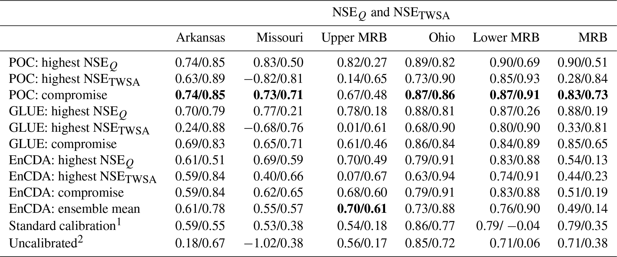
1 SL-RC and two correction factors are adjusted in 77 CDA units within the MRB, using observations of mean annual Q (calibration period 1980–2009). 2SL-RC equal to 2 and correction factors equal to 1.
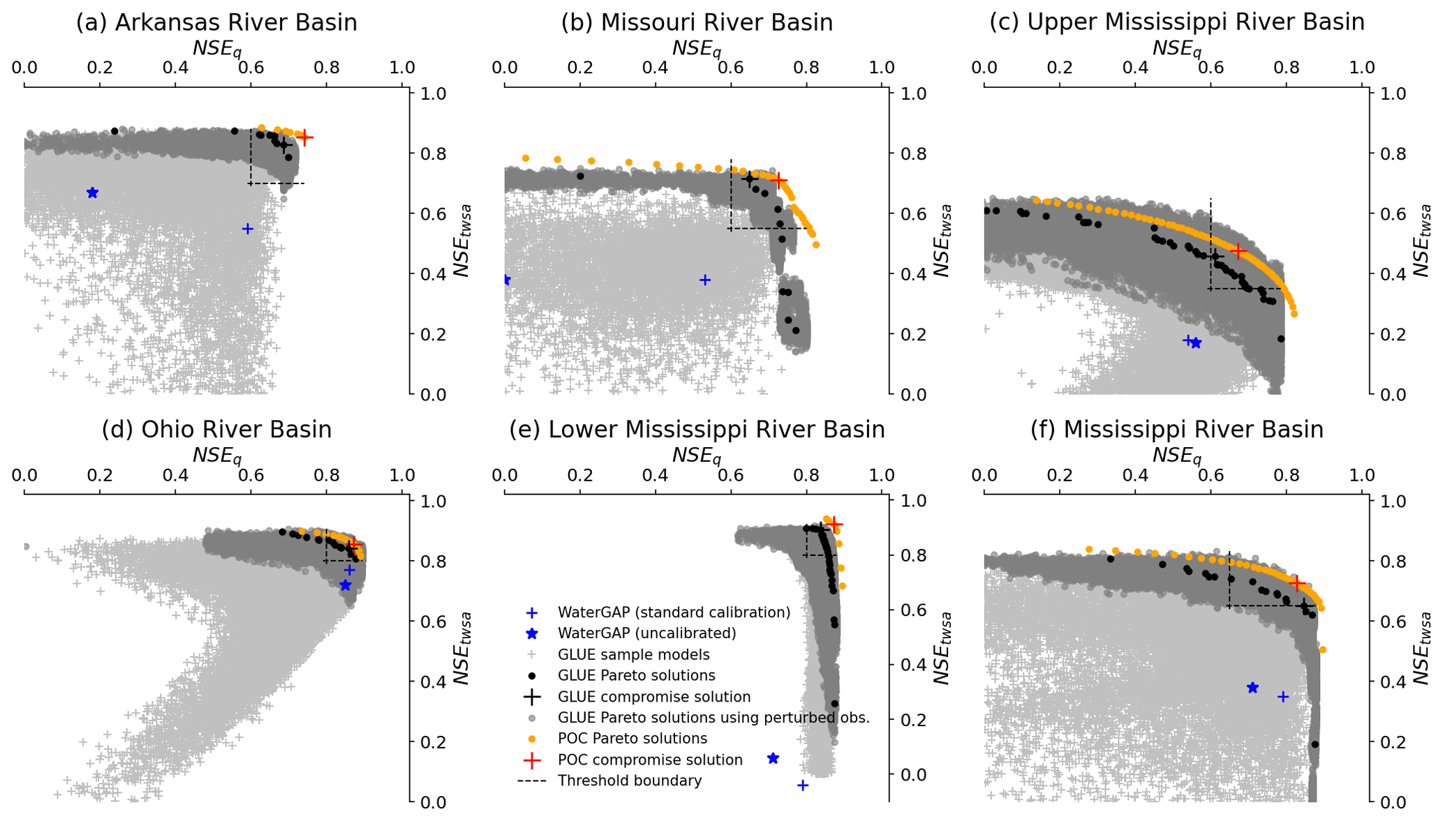
Figure 3Performance of (1) Pareto-optimal solutions derived by an evolutionary optimization algorithm (POC) (orange dots), (2) the GLUE ensemble (light-gray pluses) and (3) the Pareto-optimal subset of the GLUE ensemble (black dots); in all cases, the observation error when computing NSE is neglected. In addition, the performance of (4) the Pareto-optimal GLUE parameter subset for 1000 realizations of perturbed observations is shown (dark-gray dots), which shows the impact of observation errors on NSE. Compromise solutions of both the POC and GLUE approaches are shown too, together with the model performance after standard calibration and without calibration, consistently with Table 2. The thresholds for behavioral parameter sets (Table 3) are indicated by the dashed gray lines.
Differences between CDA units
Optimal performance strongly varies between the CDA units. The best performance with optimized parameter sets is achieved for the humid and hilly Ohio River basin and the downstream lower MRB, with NSE values exceeding 0.85 for both Q and TWSA in the POC compromise solution (Table 2). Q in the lower MRB is heavily determined by inflow from the four upstream CDA units. In the relatively dry Arkansas River basin, model performance regarding TWSA is similar to the two best-performing CDA units, but it somewhat worse regarding Q at 0.74. In the Missouri River basin and, in particular, in the upper MRB, TWSA fit to GRACE observations is worse than in the other three sub-basins. Inadequate modeling of both artificial reservoirs and wetlands is suspected to cause the low performance regarding TWSA in both basins. The Missouri River basin is the basin that is most strongly impacted by artificial reservoirs (Fig. B1a), and the parameters of the reservoir algorithm were not calibrated (see Sect. 3.2.4). The northern parts of both basins (dark-blue areas in Fig. B1c) are characterized by the existence of a high number of small wetlands, the location and extent of which are poorly quantified in WaterGAP. This stems from the classification of this whole area in the Global Lakes and Wetland Database (GLWD) (Lehner and Döll, 2004) as a “wetland complex with a 25 %–50 % coverage”, with wetlands at the maximum extent. This coarse information is included in WaterGAP by assigning a maximum extent of local wetlands of 35 % of the cell area (Döll et al., 2020). Thus, it is not only the WaterGAP algorithms for simulating the water balance of wetlands but very likely also the poor localization of wetlands that prevents parameter adjustment from resulting in good fits to observations. We speculate that, for these conditions, modification of water storages in EnCDA leads to an improved simulation of TWSA and, to a smaller degree, of Q (Table 2). In the case of the CDA unit of the MRB, where all grid cells of the whole MRB are assigned the same value in terms of the calibration parameters (Table 2), NSEQ, with a value of 0.83 for POC and GLUE, is very similar to the two best-performing sub-basins of Ohio and the lower MRB. With a value of 0.73, NSETWSA is within the range of the values of all sub-basin CDA units.
Benefits of multi-variable calibration
The performance of the compromise solutions is compared to the performances of the WaterGAP variant that is calibrated in the standard way (Sect. 3.1) and of an uncalibrated WaterGAP variant. In the standard calibration, the runoff coefficient (SL-RC) and, potentially, two correction factors are adjusted individually for each of the 77 sub-basins (CDA units) using only observations of mean annual Q at the sub-basin outlet (Figs. S2 and S3). In the uncalibrated variant, SL-RC is set to 2, and the correction factors are to 1 throughout the MRB. For all CDA units, the POC and GLUE compromise parameter sets result in higher NSE values for both Q and TWSA as compared to both the uncalibrated and the standard model variant (Table 2 and Fig. 3). This is also true for EnCDA, except for the CDA units of the MRB, where both NSEQ and NSETWSA are worse than in both the uncalibrated and standard WaterGAP variants, and the Ohio River basin, where NSETWSA is increased but NSEQ is decreased by EnCDA. In the case of the Ohio River basin, neither the standard calibration nor the POC or GLUE compromise solutions achieve a significant improvement in the already-high NSEQ of the uncalibrated model, and even the improvement in the TWSA simulation is rather small. As can be expected, the fit to the observed TWSA is improved more strongly in comparison to the standard calibration than the fit to observed Q, with the strongest improvement in the small downstream lower MRB.
Analysis of the KGE components of CC, RBias and RVar (Eqs. 3–5) (Tables B1 and B2) shows that the improved NSEQ and NSETWSA of the compromise solutions of POC, GLUE and EnCDA as compared to the standard WaterGAP results are, in all CDA units, mainly due to an improvement in the correlation (CC), the exception being NSEQ in the case of EnCDA. Thus, calibration mainly leads to improved timing of monthly streamflow and TWSA. Standard calibration only improves the bias of Q compared to the uncalibrated variant, mostly leading to an RBias value close to 1 (Table C1). The multi-variable approaches decrease the overestimation of mean annual Q by the uncalibrated model, except in the upper MRB and the Ohio River basin, where the overestimation by the uncalibrated model is already very small. However, as compared to the standard and uncalibrated model variants, none of the three calibration approaches improves the strong underestimation of Q variability by WaterGAP. Q variability in the compromise solutions becomes even more strongly underestimated in the upper and lower MRB and for the whole MRB. TWSA variability in the Arkansas and Missouri river basins and in the lower MRB is improved as compared to the standard and uncalibrated WaterGAP but is worsened in the case of the wetland-rich upper MRB (Table C2).
Overestimation of observed seasonal low flows prevails in all CDA units, not only in the compromise solutions (Figs. 3 and S4) but also in the solutions showing the highest NSEQ, while the simulation of high flows was improved by the multi-variable calibration. The improved correlation but stronger underestimation of Q variability as compared to the standard calibration can be seen in the hydrograph of observed and simulated Q for the CDA unit of the MRB for the POC and GLUE compromise solutions (Fig. 4a); the seasonal low flows are better captured with the standard calibration than with the compromise solutions. The correlation of simulated and observed TWSA is improved by achieving a small shift towards later in the year by POC or GLUE, but in some years (e.g., 2008 and 2009), the TWSA rise still occurs too early (Fig. 4b). In addition, the relatively high water storage at the end of the years of 2010 and 2011 cannot be captured by any simulation. These discrepancies in average TWSA over the MRB can be traced back to the Missouri and upper MRB sub-basins, where, in many years, simulated TWSA increases too quickly and too much in the first half of the year (Fig. S4b, d).
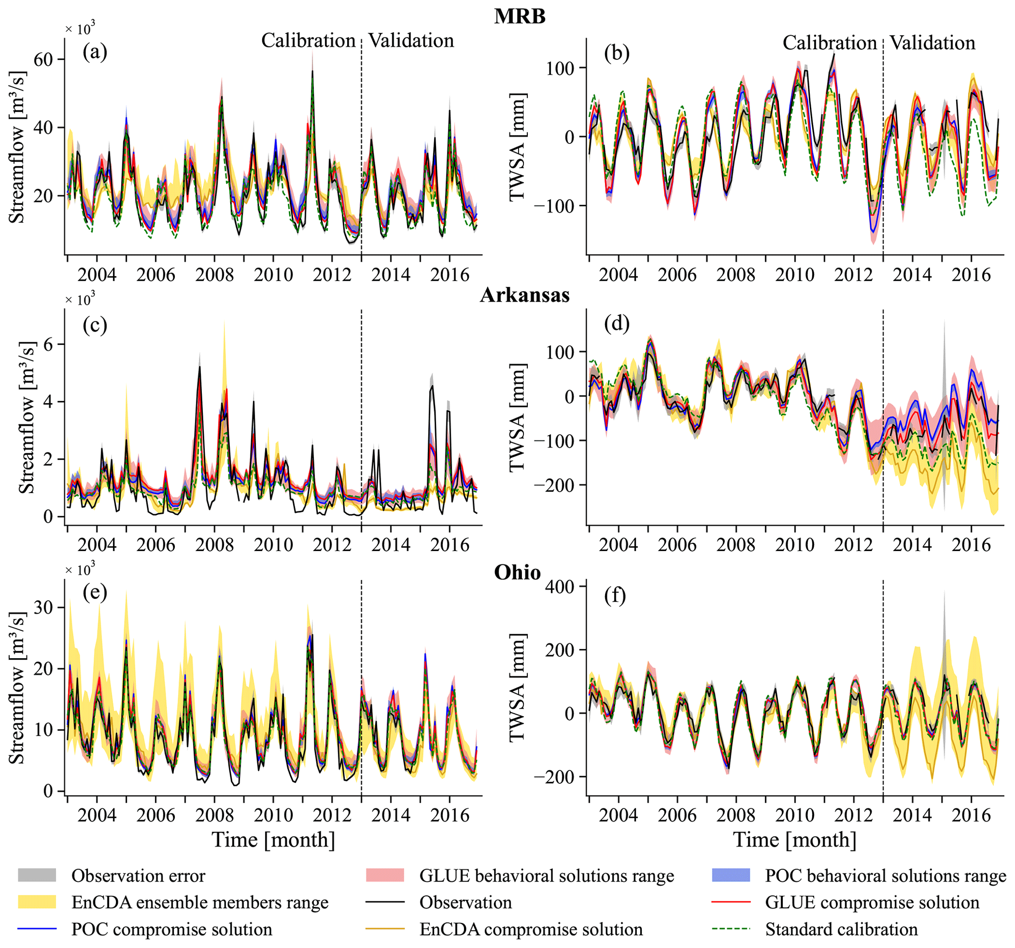
Figure 4Monthly time series of simulated and observed Q (a, c, e) and TWSA (b, d, f) during the calibration period 2003–2012 and the validation period 2013–2016 for the MRB (a, b), the Arkansas River basin (c, d) and the Ohio River basin (e, f). Observations and their assumed errors are shown together with simulated GLUE, POC and EnCDA compromise solutions, along with the range of GLUE and POC behavioral solutions (maximum and minimum monthly values of the behavioral solutions, Table 3) and the range of all 32 EnCDA ensemble members, as well as with the WaterGAP variant with standard calibration.
In the dry Arkansas River basin, all simulations overestimate summer low flows particularly strongly (Fig. 4c), while TWSA performance in the compromise solutions is much better than that of the standard WaterGAP (Fig. 4d). The Ohio River basin is the CDA unit with the best model performance and little change due to any calibration, except for a slight improvement in TWSA correlation (Fig. 4e, f). However, here, an overestimation of seasonal low flows in about half of the calibration years cannot be improved by parameter adjustment (Fig. 4e). Altogether, the visual inspection of the hydrographs of all six CDA units reveals that, even if multi-variable calibration leads to improved performance metrics, the fit to observations can only be slightly improved (mainly with respect to timing) as compared to the standard calibration (Figs. 3 and S4), except for the much-improved fit to TWSA in the lower MRB (Fig. S4f).
Trade-offs between optimal fit to Q and TWSA
Trade-offs are large for all three calibration approaches, as quantified by the NSE values for the model runs achieving the highest NSEQ and NSETWSA, except in the two CDA units with an already-satisfactory NSETWSA in the uncalibrated model variant (Arkansas and Ohio River basins). The optimal fit to observed TWSA then results in very poor fits to observed Q, in particular for the Missouri River basin and the upper MRB (Table 2). Considering POC, optimal TWSA performance leads to a stronger overestimation of mean Q of 27 %–73 % as compared to 1 %–18 % in the case of optimal Q performance (excluding the downstream lower MRB) (Table C1). While the ratio of the simulated to observed variability of TWSA decreases and thus improves, the corresponding ratio for Q decreases too but, as a result, becomes worse. RVarQ ranges from 0.80 to 0.88 in the case of maximum NSEQ and decreases to the range of 0.53–0.84 in the case of maximum NSEQ (except for the Arkansas River basin). Considering POC in the Missouri River basin as an example, the parameter set with the best fit to observed TWSA results in NSETWSA of 0.81 but a negative NSEQ; the parameter set with the best fit to Q achieves an NSEQ of 0.83, but NSETWSA deteriorates to 0.50 (Table 2). The parameter set with an optimal fit to TWSA leads to an even higher overestimation of mean Q (RBias = 1.73) and an even higher underestimation of Q variability (RVar = 0.61) as compared to the ensemble member with the best fit to observed Q (RBias = 1.08, RVar = 0.80), while the correlation slightly decreases (Table C1). KGE components regarding TWSA for the same CDA unit reveal that the correlation of observed and simulated TWSA strongly decreases from 0.91 to 0.77 if optimization is done for Q instead of TWSA, while variability is overestimated somewhat more (RVar = 1.09 instead of 1.03) (Table C2). Similar patterns are observed for the CDA units of the MRB and upper MRB. In the case of the Arkansas River basin and the lower MRB, trade-offs between optimal fits to Q and TWSA observations identified by POC are lower than those identified by GLUE, which shows the advantage of the search algorithm applied in POC.
4.1.2 Behavioral parameter sets
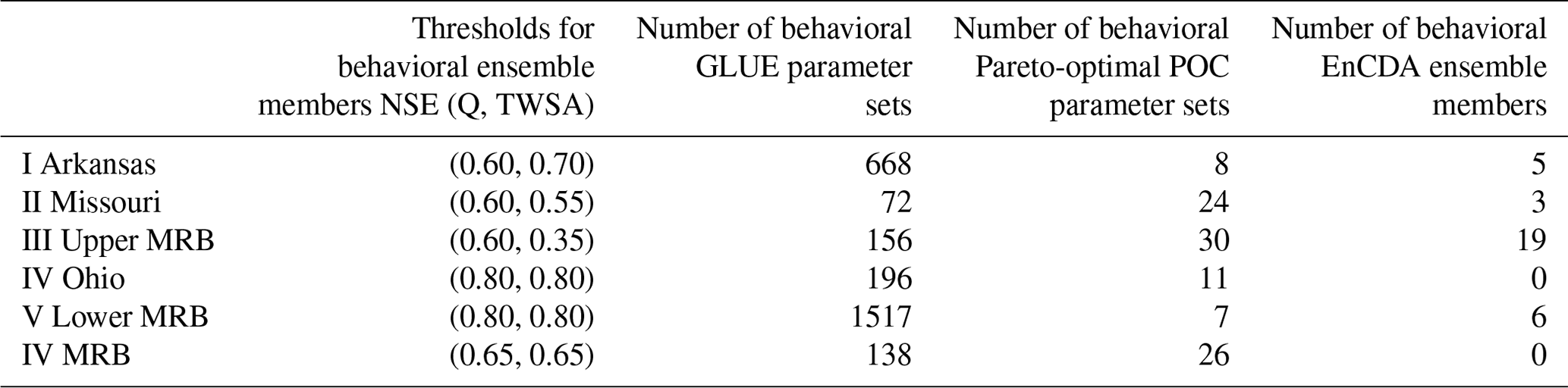
We identified behavioral parameter sets using thresholds for the minimum acceptable performance in terms of NSEQ and NSETWSA, taking into account the observation uncertainties of Q and TWSA. To do this, we evaluated the performance of the 20 000 simulated GLUE ensemble members with respect to uncertainty-perturbed observations (Figs. 3 and S1), as described in Sect. 3.4.2. For GLUE and EnCDA, all parameter sets within the thresholds were selected as behavioral, while for POC, the behavioral parameter sets are the subset of Pareto-optimal parameter sets above the thresholds. The Pareto-optimal GLUE model runs for 1000 perturbed observation time series (dark-gray dots in Fig. 3) served to assess the impact of observation uncertainty on performance. Not every dark-gray dot represents a different parameter set because the NSE for the same parameter set varies with the perturbed observation time series. The width of the band of the Pareto-optimal model runs in the case of perturbed observations close to the compromise solution helped to identify the thresholds for NSEQ and NSETWSA. In the case of the poorly simulated upper MRB, we decided to keep the thresholds above those indicated by the observation error analysis to avoid calling very poorly performing parameter ensembles behavioral (Fig. 3). We chose the compromise solution as the point of departure as we wish to give equal weight to the performances of Q and TWSA. Thresholds for behavioral parameter sets vary between the CDA units due to the different optimal performances that can be achieved, in the different CDA units, by varying parameters given a fixed model structure and the model input. The selected thresholds for behavioral solutions are indicated in Fig. 3 and Table 3, while Table 3 also provides the number of behavioral POC and GLUE parameter sets, as well as the number of the behavioral EnCDA ensemble members.
Table 3Number of identified behavioral parameter sets (or ensemble members) for each CDA unit that lead to simulation results that exceed both the NSEQ and NSETWSA thresholds. Listed are the number of behavioral parameter sets in the GLUE approach (out of 20 000 per CDA unit), the number of behavior Pareto-optimal parameter sets in the POC approach (out of 20 000) and the number of behavioral EnCDA ensemble members (out of 32).
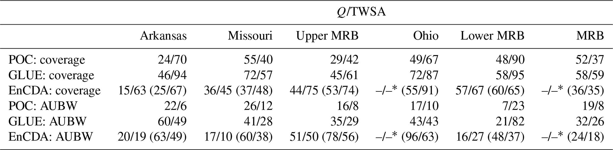
In the case of POC and GLUE, an uncertainty band is delineated by the minima and maxima of monthly Q or TWSA values when considering all behavioral parameter sets (Figs. 3 and S4). For EnCDA, these figures also show the range of all 32 ensemble members because there are no behavioral EnCDA members in the case of the CDA units of the Ohio and MRB. AUBW and coverage of observations (including their uncertainty) by the uncertainty band of the model output can be expected to correlate (Sect. 3.3). Both AUBW and the coverage are smaller for POC and EnCDA than for GLUE (Table 4) due to their smaller number of behavioral ensemble members. When extending the considered EnCDA ensemble members to the whole ensemble of 32 members, the coverage increases slightly, but at the same time, the width of the uncertainty bands increases strongly (Table 4). Comparing the six CDA units, neither AUBW nor coverage correlate with the number of behavioral ensemble members.
Table 4Coverage of monthly observations by model output (CO) in percentages (%) of monthly observations contained in the uncertainty band of observations and average uncertainty bandwidth AUBW during the calibration period 2003–2012 for both Q and TWSA considering only the behavioral parameter sets (Table 3). In the case of EnCDA, the values for the whole ensemble of 32 members are also shown in parentheses. AUBW for Q is listed in percent (%), and AUBW for TWSA is in millimeters (mm).
* No behavioral parameter sets identified.
For POC and GLUE, the average width of the uncertainty bands for Q in the six CDA units is 7 %–26 % and 21 %–60 % of the ensemble mean of monthly Q, respectively. For GLUE, the lowest AUBW occurs in the downstream lower MRB, likely due to the dominance of inflow from upstream, and the highest occurs in the Arkansas River basin (Table 4). However, even the wider GLUE bands do not cover most of the observed seasonal low flows (including the rather small observation error bands) in all CDA units, while high-flow months are covered more often (Figs. 3 and S4). Coverage in the GLUE approach ranges from 46 % to 72 % of the observed Q values among the six CDA units, with the lowest values for the two CDA units with the highest underestimation of Q variability, the Arkansas and upper MRB, even though the Arkansas River basin has the widest uncertainty band.
Coverage of observations, including their error range by the uncertainty band, is, in the case of GLUE and POC, higher for TWSA than for Q, except for the Missouri and MRB (Table 4). In the case of GLUE, TWSA coverage ranges from 59 % to 95 %. The Arkansas River basin has a low Q coverage but a very high TWSA coverage, while the Missouri River basin has the highest Q coverage and the lowest TWSA coverage, even though, for the Missouri River basin, the Q performance of the compromise solution is relatively poor (Table 2). The TWSA time series for the Arkansas River basin differs from those of the other CDA units in terms of its high ratio of interannual to seasonal variability (Fig. 4).
4.2 Model performance during the validation period 2013–2016
Model performance of both the POC and GLUE compromise solutions in the validation periods is similar to that in the calibration periods regarding Q but much worse regarding TWSA (compare Table 5 to Table 2 for NSE values). For most CDA units and calibration approaches, the performance loss regarding TWSA between the calibration and the validation period is similarly high for the ensemble members that were identified as having the best fit to TWSA. We suspect that the poor fit of simulated TWSA to observed TWSA in the last years of the GRACE mission, where there is also a large fraction of missing monthly GRACE data (Figs. 3 and S4), is related to increased observational errors (compare Sect. 3.2.2). This suspicion is supported by the fact that the NSETWSA of the uncalibrated model is lower for the validation period than for the calibration period, which is not the case for NSEQ in all CDA units except the Arkansas River basin.
Table 5Model performance during the validation period 2013–2016 indicated by NSEQ and NSETWSA, as achieved by the three calibration approaches (POC, GLUE and EnCDA) as well as by the standard WaterGAP 2.2d and the uncalibrated WaterGAP 2.2d models. The best-performing calibration approach per CDA unit, with the highest average NSE, is indicated in bold. The indication “highest NSETWSA” refers to the parameter with the best performance during the calibration period. The values in parentheses in the line “EnCDA compromise” are NSETWSA values that are computed after normalizing TWSA during the validation period by the mean TWSA of the validation period.
1 Computed by running WGHM with the ensemble of behavioral Pareto-optimal parameter sets identified using POC (Table 3). 2 Computed by running WGHM with the ensemble
of behavioral parameter sets identified using GLUE (Table 3). 3 Computed by running WGHM with the ensemble of 32 parameter sets identified using EnCDA (Sect. 4.1.3).
All compromise solutions perform somewhat better than the WaterGAP standard variant, except for EnCDA in the CDA units of the Missouri, Ohio and MRB (Table 5). Performances of the ensemble mean of the behavioral GLUE parameter sets, the ensemble mean of the behavioral Pareto-optimal POC parameter sets and the EnCDA ensemble mean are similar to their respective compromise solutions (Table 5). In all CDA units, POC and GLUE perform better than EnCDA regarding both Q and TWSA. POC results are slightly better than GLUE results, with the exception being the Arkansas River basin, where POC performance regarding TWSA degrades from its high level during the calibration period due to overestimation of the mean TWSA (Fig. 4).
The temporal mean value of GRACE-derived TWSA is generally unknown. The standard approach taken in this study of normalizing TWSA values to a constant mean over the reference period, here 2003–2012, may be problematic as it assumes that the mean derived over longer periods than the reference period (here 11 years) remains at the reference period value, which need not be true. Therefore, we additionally calculated, for the example of the EnCDA compromise solution, the NSETWSA after reducing the TWSA time series by its temporal mean of the validation period instead of the mean of the calibration period. The resulting NSETWSA values are, for most CDA units, somewhat improved (Table 5).
4.3 Characterization of estimated parameter sets
POC and GLUE identify parameter sets that are assumed to be temporally constant. Here, we compare these two ensembles of estimated parameter sets. Starting with the CDA unit MRB, we first characterize the parameter sets of the POC compromise solution and the parameter sets leading to the best fit to either Q or TWSA. We compare the parameter set of the GLUE compromise solution to the parameter set of the POC compromise solution. Then, we describe the POC behavioral Pareto-optimal parameter sets, as well as the GLUE behavioral parameter sets, including parameter correlations. Finally, we highlight the most interesting results for the five sub-basin CDA units. The EnCDA parameter sets are not considered as the EnCDA approach leads to a lower model performance than POC and GLUE.
4.3.1 CDA unit MRB
Parameter set of the POC compromise solution
In the compromise solution, the runoff coefficient (SL-RC) is close to the maximum value of 3, minimizing runoff at a given soil water saturation (Fig. 5f). This SL-RC is in line with the values obtained by the standard calibration, where calibrated SL-RC values are also very high (Fig. S3b). While, in the standard calibration, one or two correction factors are needed in most standard-calibration CDA units to decrease mean annual runoff to the observed values, this is achieved in this study by a high value of SL-MSM, the multiplier for the standard maximum soil water storage, which is adjusted in the POC compromise solution to a high value of 2.5. A “deeper soil” with higher water storage capacity leads to decreased soil saturation and lower runoff and, at the same time, to higher variability in terms of soil water storage and, thus, TWSA. EP-PTh, affecting potential evapotranspiration, is reduced from its standard value of 1.26 to 1.02, which seems to contradict the adjustment of both SL-RC and SL-MSM as this should lead to a reduction in actual evapotranspiration and thus an increase in runoff, in particular at high soil saturation values (Eq. 17 in Müller Schmied et al., 2021).
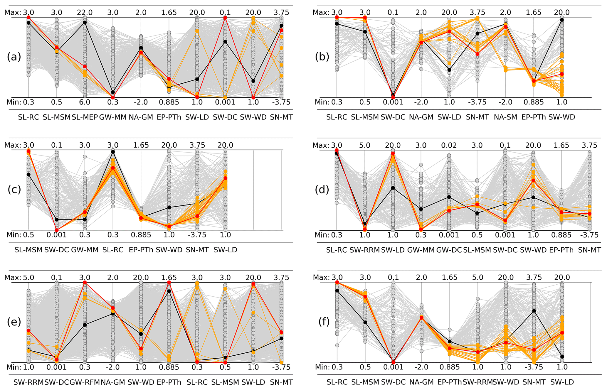
Figure 5Parameter sets determined by POC and GLUE calibration approaches as depicted by parallel coordinate plots for the CDA units of (a) Arkansas, (b) Missouri, (c) upper MRB, (d) Ohio, (e)lower MRB, and (f) MRB. The parameter abbreviations are given at the bottom of each plot, where the order was selected to show interesting relations between parameter values. The numbers at the top and bottom of the plots indicate the a priori range of the calibration parameters listed in Table 1. The number of behavioral solutions is given in Table 3. GLUE behavioral solutions are shown in gray, the GLUE compromise solution is in black, the POC Pareto behavioral solutions are in orange, and the POC compromise solution is in red.
In addition to SL-MSM, three other parameters are adjusted by the calibration in a way that water retention is increased (improving correlation with both observed Q and TWSA), while, at the same time, a higher TWSA variability results (decreasing or at least not improving the fit to the observed Q and TWSA). Both maximum wetland (SW-WD) and lake depths (SW-LD) are increased by calibration, from 2 to 5.7 m in the case of wetlands and from 5 to 8 m in the case of lakes, and the lake and wetland discharge coefficient (SW-DC) is adjusted to its minimum value of 0.001 d−1. In contrast, the adjustment of the river roughness coefficient multiplier (SW-RRM) to 1.5, i.e., to half of the value in the uncalibrated model, leads to a doubling of the flow velocity in the river as compared to the standard value and, thus, lower water retention (reducing the correlation with observed Q and TWSA), a higher variability in terms of Q (improving the fit to observations) and a higher variability in terms of TWSA (worsening the fit to observations). In addition, the net abstraction from groundwater is decreased by 80 % (NA-GM = 0.2). Snow melt temperature (SN-MT) is lowered from the standard value of 0 to −2.6 °C with POC. Overall, most parameters are adjusted to increase the correlation between observed and simulated TWSA (except for SW-RRM) and to reduce the mean runoff (except for EP-PTh). Unfortunately, the adjusted parameters increase TWSA variability (except for SW-RRM), leading to an even stronger overestimation than for the uncalibrated and standard calibrated variants (Table C2) and a worse underestimation of Q variability (Table C1).
Parameter sets with optimal fit to Q or TWSA for POC
Regarding trade-offs, the POC parameter set that leads to the best fit to observed Q is characterized by a higher SW-RRM (2.2 instead of 1.5 in the compromise parameter set), a two-third reduction in SW-LD, a higher SN-MT and a value of NA-GM of approximately 1. The latter shows that the net groundwater abstractions estimated by the water use models of WaterGAP lead to a good fit for the monthly Q time series. In the POC parameter set leading to the best fit to observed TWSA, SL-MSM reaches 3 (the maximum value), while SW-WD attains a value of more than 12 m. This parameter set includes an SW-RRM value of only 1 (the lower bound, leading to a minimum flow velocity) and a slightly negative NA-GM. The latter parameter value means that the net water abstractions from groundwater, which are dominantly positive in the MRB (Fig. B1e) – i.e., more water is withdrawn from the groundwater than recharged by return flows – are not only decreased but become mostly net groundwater recharge through the parameter adjustment. This could be caused, for example, by an original overestimation of the fraction of the total water abstraction that stems from groundwater and not surface water. Return flow from irrigation with surface water can lead to a net abstraction from groundwater that is negative, i.e., an artificial groundwater recharge. However, this might also be caused by an underestimation of groundwater recharge, such that groundwater storage loss and the decrease in groundwater outflow to rivers by net groundwater abstractions would be overestimated if NA-GM was not adjusted from its standard value of 1.
Parameter set of the GLUE compromise solution
Six out of the nine parameters in the GLUE compromise solution are very similar to those of the POC compromise solution (Fig. 5f). The GLUE compromise solution has a slightly higher NSEQ but a considerably lower NSETWSA (due to a lower correlation but a similar performance of variability) due to a lower soil moisture capacity and a very minimum lake water storage. In addition, the snow melt temperature is much higher.
Behavioral Pareto-optimal POC parameter sets
The 26 behavioral Pareto-optimal parameter sets derived by POC coincide in the four parameters SL-RC, SL-MSM, SW-DC and NA-GM (Figs. 5f and 6 and Excel file in the Supplement). The parameter values of the other five parameters diverge somewhat, indicating conflicts between a good fit to observed Q and TWSA. The fit to Q decreases, and the fit to TWSA increases with decreasing EP-PTh, SN-MT and SW-RRM and with increasing SW-WD. A negative correlation is visible between the values for SW-WD (wetland depth) and the values for SW-LD (lake depth) (see also Fig. S5f); this indicates that the same impact on Q and TWSA is achieved by either a large wetland depth or a large lake depth. The negative correlation between SW-WD and the three parameters EP-PTh, SW-RRM and SN-MT is not easily interpretable (Fig. S5f).
Behavioral GLUE parameter sets
Behavioral GLUE parameter sets are much more diverse than behavioral Pareto-optimal parameter sets (Figs. 5f and 6). The GLUE parameter sets take into account, in an approximate manner, the uncertainty of performance indicators that stems from observation errors (Sect. 3.2.2 and 3.4.2), in addition to the conflicting goals of achieving a good fit to observed Q and observed TWSA that is also reflected by the Pareto-optimal parameter sets. The 138 behavioral GLUE parameter sets, which all result in NSE values > 0.65, vary widely and, for some parameters, cover the whole parameter range (Figs. 5f and 6). In most behavioral sets, the SL-RC values are larger than 2, but there is even a set with a value below 1. SL-MSM ranges between 1 and 2.7, while the parameter value of the POC compromise solution is at the upper end of this range. Differently from the Pareto-optimal POC solutions, SW-RRM values do not encompass very small values close to 1 but tend to be higher, mostly between 2 and 3 (Fig. 6). SN-MT and the three parameters related to lakes and wetlands, namely SW-DC, SW-LD and SW-WD, are not constrained at all by the calibration (Figs. 5f and 6). Parameter correlations are very low, except for negative correlations of EP-PTh with SL-RC, NA-GM and SW-DC (Fig. S5f).
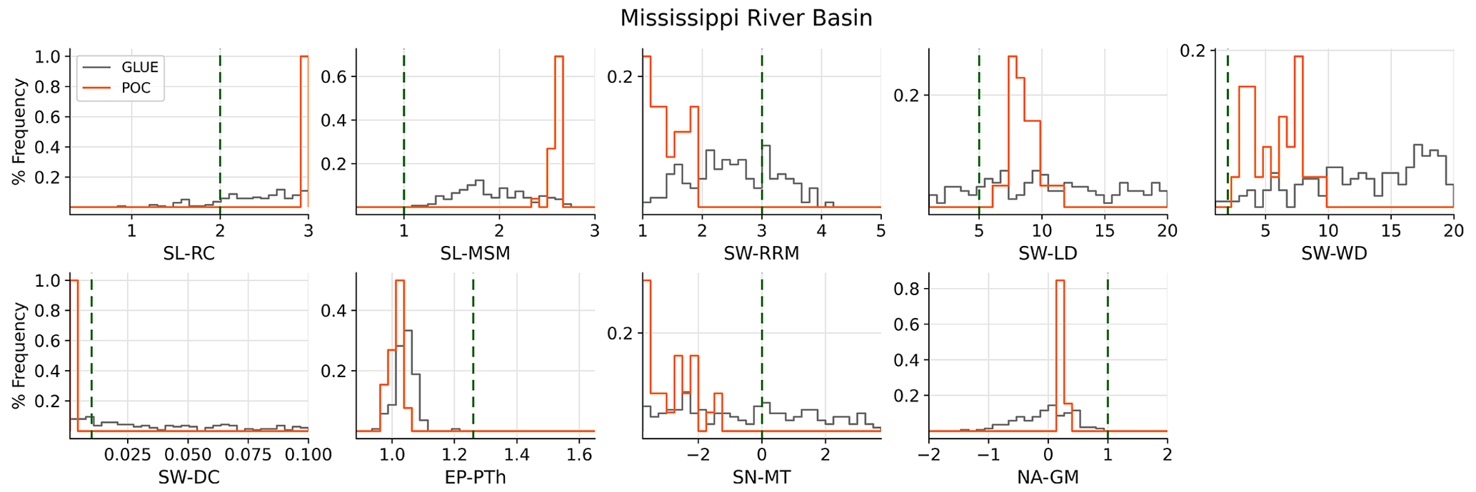
Figure 6Histogram of parameter values in calibrated parameter sets according to POC and GLUE for the MRB (CDA unit VI). All behavioral parameter sets are considered for GLUE, while the smaller ensemble of behavioral Pareto-optimal parameter sets is shown for POC (Table 3). The y axis shows the ratio of the number of parameter values in each class to the total number of behavioral parameter sets, while the x axis shows the a priori parameter range listed in Table 1. The dashed green line indicates the parameter values of the uncalibrated WaterGAP model.
4.3.2 The five sub-basin CDA units
For all five sub-basins, except the downstream lower MRB (with SL-RC = 0.33), calibrated SL-RC is close to the maximum value of 3 in the POC compromise solution (Fig. 5). SL-MSM is at its lower bound in the lower MRB but is larger than 1 in all other CDA units; the multiplier is almost at its maximum value of 3 for the Missouri River basin and the upper MRB; at about 2 for the Arkansas River basin; and at 1.3 for the Ohio River basin, which is the basin with the best performance of the uncalibrated model. In all CDA units but the Arkansas River basin, SW-LD reaches very high values between 10 and 20 m, and SW-WD is also higher than the uncalibrated values in all CDA units except the Arkansas and upper MRB. The SW-DC is at its minimum value in the Missouri River basin and the upper MRB, close to its uncalibrated value in the Arkansas and Ohio river basins, and in between in the lower MRB. Calibrated SN-MT varies strongly among the CDA units. NA-GM is always below 1 to increase groundwater retention. The lower MRB is the only CDA unit where optimal EP-PTh was high (1.65), while, in all other CDA units, the calibrated value was close to 1.
Overall, there is a particularly high equifinality of parameter sets in the lower MRB, with strong negative correlations between parameters of the Pareto-optimal POC solutions (Fig. S5e). Among the POC solutions in the Arkansas River basin, the parameters of wetland depth (SW-WD) and surface water discharge coefficient (SW-DC) (Fig. 5a – compare POC compromise solution with POC behavioral solutions – and Fig. S5a) are so negatively correlated that the parameters alternatively take values at the opposite limits of the parameter ranges. A high value of maximum storage in surface waterbodies has a similar effect on Q and TWSA dynamics as a low surface water discharge coefficient that keeps water in storage. Parameters may also show very strong correlations within a very small parameter space, as in the case of EP-PTh and SW-WD in the upper MRB (Figs. 5c and S5c).
The GLUE behavioral parameter sets cover an even larger range in the lower MRB and the Arkansas River basin as compared to the MRB (Figs. 5 and S7). Correlations between parameters are generally low (Fig. S6), except for high negative correlations between EP-PTh and SL-RC in the Missouri River basin and between EP-PTh and SL-MSM in the Ohio River basin. However, low correlations between the calibrated parameters do not indicate a low equifinality.
4.4 Added value of spatially more resolved CDA units
An important decision in model parameter estimation is the choice of CDA units, i.e., the selection of the group of grid cells for which calibration parameters are assumed to be the same. A higher number of CDA units within the same geographic domain leads to the adjustment of more parameters, causes a higher computational effort and is expected to lead to an improved representation of reality. We performed two analyses to evaluate the added value of dividing the MRB into five sub-basin CDA units.
In the first analysis, we used the compromise solutions obtained for the CDA unit VI (MRB), where the same calibration parameter values are assigned to all grid cells in the whole MRB, to compute Q and TWSA for each of the five sub-basin CDA units. Model performance of this calibration variant (“whole-basin calibration”) is compared to the performance that is achieved in the sub-basins if each sub-basin is calibrated individually, i.e., if five CDA units are used to cover the whole MRB. Analysis for both the calibration period (Table 6) and the validation period (Table S3) clearly shows the added value of distinguishing five sub-basin CDA units (calibration variant “sub-basin calibration”) as overall model performance improves in each of the five sub-basins as compared to the calibration variant “whole-basin calibration”. Due to the specific search algorithm, performance gains are more pronounced with POC than with GLUE. Performance gains are very high in the case of EnCDA due to the poor performance of the whole-basin calibration. Considering POC and regarding Q, the added value of more CDA units is highest for the Missouri River basin, followed by the Arkansas River basin and the upper MRB. However, for these three sub-basins, there is no added value regarding TWSA. In the always-best-performing Ohio River basin, there is a small added value for both Q and TWSA, while in the downstream lower MRB, where Q is dominated by inflow from the four upstream sub-basins, Q performance remains essentially unchanged, while TWSA performance improves with more CDA units.
Table 6Comparison of model performance in the five sub-basins of the MRB between the calibration of MRB as a whole (only CDA unit VI) and calibration of the individual sub-basins (five CDA units I–V). In addition, the performance of the model with standard calibration of 77 CDA units but adjusting only up to three parameters based on observed mean annual Q is shown. Model performance is indicated by NSEQ and NSETWSA during the calibration period 2003–2012 as achieved by the compromise solutions of the three calibration approaches POC, GLUE and EnCDA. The sub-basin calibration NSE values are identical to those in Table 2, except for MRB (see footnote 1).
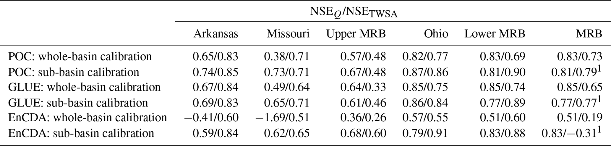
1 Based on Q at Vicksburg and TWSA averaged over the whole MRB computed by a WaterGAP run, in which the calibration parameters in the five sub-basins (CDA units I–V) were set to their respective compromise solution values.
An evaluation of the performance regarding the mean of TWSA over the entire MRB using the individual parameter sets of the five sub-basin CDA units shows a small added value of using sub-basin CDA units in the case of POC and GLUE, while, in the case of EnCDA, the already-poor fit to TWSA in the whole-basin variant is further degraded (column MRB in Table 6). However, EnCDA estimation of Q at Vicksburg is much improved with five CDA units and reaches the high values of GLUE and POC, both of which show a slight degradation in the Q simulation at Vicksburg as compared to the whole-basin calibration.
In the second analysis, we evaluated the ability of the different calibration variants to simulate Q at six Q gauging stations that were not used for model calibration in this study; three are located in the Missouri River basin, and three are located in the Ohio River basin (Fig. 2). Differences between the stations are larger than between the calibration approaches. Good NSEQ values are only achieved at two stations, Mt. Carmel and Louisville in the Ohio River basin. The best performance at Mt. Carmel is achieved with the whole-basin GLUE approach (NSE = 0.77), while the POC sub-basin approach achieves the optimal performance at Louisville, with NSE = 0.91 (Table 7). Sub-basin calibration strongly improves NSE as compared to whole-basin calibration in the case of the Platte River station at Louisville for both POC and GLUE by reducing the bias (RBias) but decreasing correlation (CC) and the fit to observed Q variability (RVar) (Table 7) but not during the validation period (Table S4). There is some added value in the sub-basin calibration regarding Q simulation at the Louisville station on the Ohio River for both the calibration and the validation period. For the other four stations, however, sub-basin calibration leads to worse performance than whole-basin calibration during the calibration period. For the station on the Cumberland, which is not a calibration station in the standard calibration, the standard calibration even leads to a better performance than all the ensemble-based calibrations for both the calibration and validation period. At the Bismarck station on the Missouri River, where model performance is similarly poor compared to that on the Cumberland, even the uncalibrated WaterGAP variant performs better or similarly to the calibrated variants due to the highest correlation. During the validation period, the performance of all three calibration approaches becomes very low at the three stations in the Missouri River basin (Table S4), while it remains constant or even improves for the three stations in the Ohio River basin. No calibration approach performs consistently better than any other approach; performance rather depends on the period and the station. Overall, calibration using Q observations on downstream stations only leads to apparently random changes in Q simulation at upstream stations that have not been used in the calibration.
Table 7Comparison of model performance at the six Q validation stations in the Missouri and Ohio sub-basins of the MRB (Fig. 2) between the calibration of the MRB as a whole (CDA unit VI) or calibration of the individual sub-basins (CDA units I–V). Model performance is indicated by NSEQ and the three KGE components during the calibration period 2003–2012 as achieved by compromise solutions of the three calibration approaches POC, GLUE and EnCDA. In the case of EnCDA, the performance metrics for the 2003–2012 CDA run are shown, and those of a run with the parameter set of December 2012 are not shown. The best-performing calibration variant for each station is shown in bold. In addition, performances of the standard and uncalibrated WaterGAP model variants are shown.
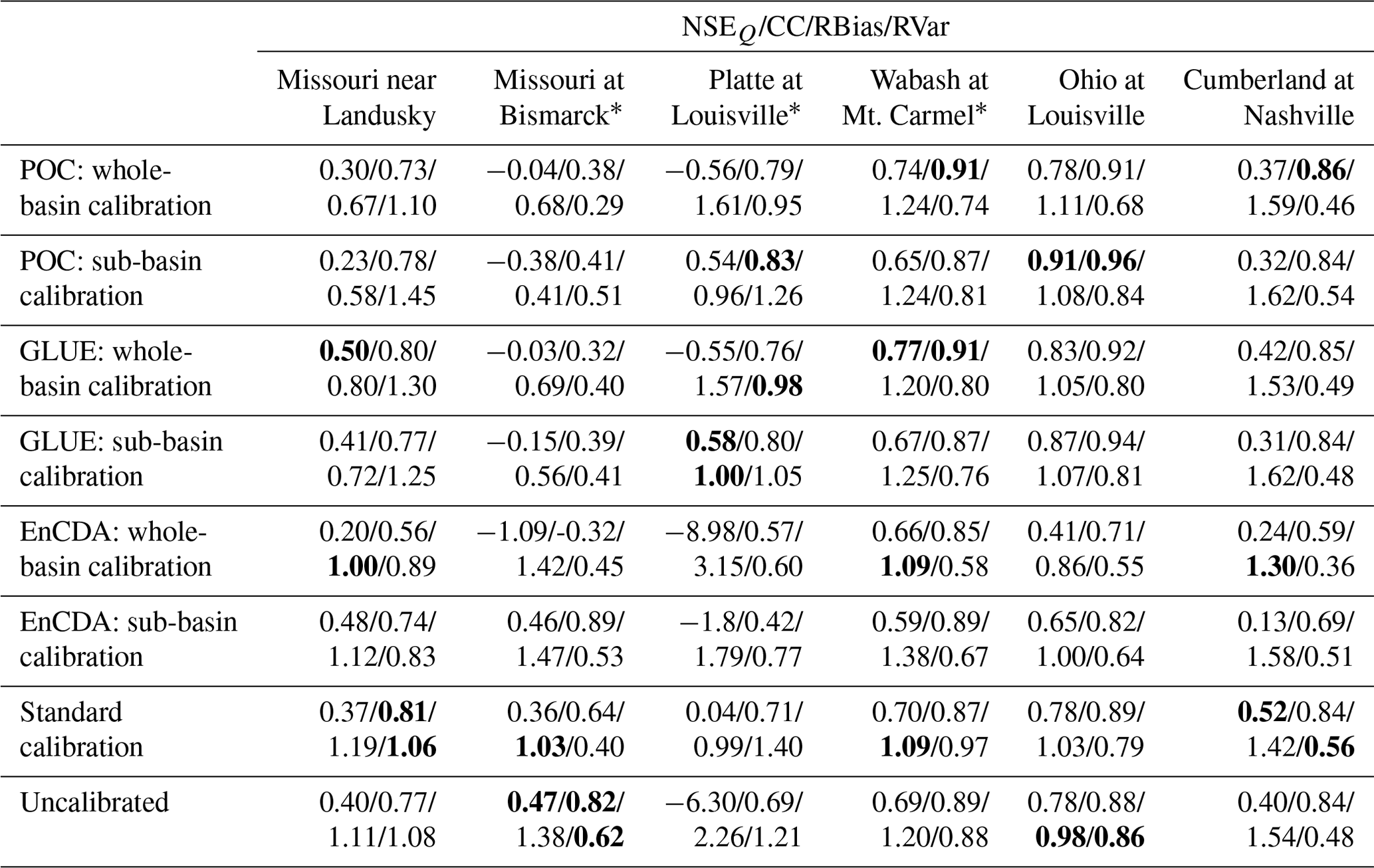
* Calibration station of standard calibration.
5.1 Advantages and disadvantages of the three ensemble-based multi-variable calibration approaches
POC is most effective in reducing the uncertainty of GHM model output by identifying (Pareto-) optimal parameter sets or one compromise parameter set that leads to the overall best fit to all observation variables. However, we found in our study that GLUE is only slightly less effective in doing this; the differences between the time series of Q and TWSA computed by POC and GLUE are small compared to the discrepancies between the simulations and the observations (Figs. 3 and S4). The major advantage of GLUE is that, without any additional model runs, the GLUE parameter ensemble can also be used to identify behavioral parameter sets and thus quantify the model output uncertainty given the uncertainty of the observations. In addition, GLUE has a smaller computational burden than POC if alternative calibration objectives are to be tested as no new model runs are required in the case of GLUE. The computational burdens of POC and GLUE, which are dominated by the number of parameter sets used to compute the alternative model output, are rather similar (Sect. 3.4.1 and 3.4.2).
Theoretically, EnCDA is, similarly to GLUE, capable of both decreasing and quantifying the uncertainty of GHM model output. However, unlike POC and GLUE, the “best estimate” of model output in ensemble Kalman filter methods is not connected to one specific parameter set but is determined by the mean over the outputs of all ensemble members, which are also affected by the forcing perturbations. Therefore, consistent simulations with an EnCDA-calibrated model, e.g., for a period without observations, such as the validation period in our study, require that the model is not only run once but rather, with the parameter values obtained at the end of the calibration period, as many times as the ensemble has members (32 times in our study, Sect. 3.4.3). These ensemble runs then enable us to compute a best estimate and an uncertainty band that takes into account the uncertainty of the observations and the model, as well as of some climate input. However, as EnCDA does not compute a single optimal parameter set but rather a Bayesian mean, it seems to be less straightforward to use it for many model applications. In the case of POC and GLUE, the model needs to be run only once, with the compromise parameter set, to obtain the best estimate of model output given the observations used for model calibration.
The fact that our EnCDA implementation could not compete with POC and GLUE in simulating Q and TWSA during the calibration period might be viewed as surprising as, in EnCDA, it is not only parameters but also water storages that are adapted each month. We believe that the lower EnCDA performance is due to the small ensemble size of only 32 (instead of 20 000 in the case of POC and GLUE); it is common in EnKF data assimilation to only generate very small ensembles (e.g., Zaitchik et al., 2008; Eicker et al. 2014; Girotto et al., 2016; Kumar et al., 2016), which is caused by the high computational demand of the EnCDA approach. This is because EnCDA estimates state parameters and can run recursively, i.e., providing state and parameter estimates at every time step, which POC and GLUE cannot do. With gradually increasing ensemble sizes (e.g., n=64), one generally finds gradually improved state and parameter estimates, but the EnCDA will never be able to be run with ensemble sizes common in model calibration. Put in other words, the EnCDA allows for many more degrees of freedom as compared to POC and GLUE since it does not assume the model itself to be correct but rather only ambiguous due to unknown model parameters. We caution that EnCDA using only one CDA unit for the whole MRB even failed in the sense that it resulted in a worse performance in terms of NSE regarding both Q and TWSA than the uncalibrated WaterGAP during the calibration period 2003–2012. Regarding the five sub-basin CDA units, the performance for all but one CDA unit was worse than that of POC and GLUE even though it is not only parameters but also water storages that are adjusted in EnCDA. Performance was, however, improved over the standard and uncalibrated model variants for four out of six CDA units, in particular regarding TWSA. Q simulation by EnCDA during the calibration period might be improved by using log Q instead of Q (Clark et al., 2008; Paiva et al., 2013) and, in the case of dry world regions, by censoring no-flow observations (Wang et al., 2020). Note that we define performance generally in terms of NSE, while EnCDA, unlike POC and GLUE, does not optimize NSE but rather does so for the RMSE of model–observation differences. In the validation period 2013–2016, when EnCDA uses the 32 parameter sets obtained at the end of the calibration period (December 2012) to compute Q and TWSA without any update to water storages, TWSA and, to a lesser extent, Q “drift off” from the observations, resulting in very poor fits. This may be explained by the fact that the monthly parameter updates in EnCDA absorb model misrepresentations that generate seasonally varying errors such that the December 2012 parameter sets were not able to lead to a reasonable simulation during the entirety of the 4 years of the validation period. From a data assimilation perspective, where the aim is only to improve the knowledge about historical conditions, our validation experiment can be viewed as academic since there would be no reason not to recursively assimilate more recent TWSA observations once an ensemble assimilation framework has been set up and tuned.
5.2 Added value of multi-variable calibration as compared to the standard WaterGAP calibration for identifying one optimal parameter set
The optimal or compromise parameter sets identified by multi-variable calibration with all three approaches result in better simulations of both Q and TWSA during the calibration period as compared to the standard WaterGAP for all six CDA units, except for EnCDA in the case of the whole MRB (Table 2). However, the added value of any calibration is very low in the humid and hilly Ohio basin, where the performance of the uncalibrated model is already good; in their study on calibrating the VIC model for the USA using observed Q only, Troy et al. (2008) also found that modeled streamflow that fit well to observations before calibration, as was the case for the Ohio River, continued to do so.
As expected, the improvement in TWSA simulations is more pronounced than the improvement in Q. Higher NSEQ values are mostly caused by improved correlation, while Q variability is still underestimated and low flow is overestimated in all CDA units, and in three CDA units, this is even more strongly the case than for the standard and uncalibrated WaterGAP variants. In two CDA units, the mean Q is overestimated by more than 10 % (Table C1). The much higher NSETWSA values of the compromise solutions as compared to standard WaterGAP are also mainly caused by much-improved correlations, with improved or worsened TWSA variabilities depending on the CDA unit (Table C2). The analysis of model performance at the same observation locations for the validation period 2013–2016 confirms the added value of POC and GLUE.
However, visual inspection of the hydrographs for both the calibration and validation periods reveals that the fit to observations can only be improved slightly by the multi-variable calibration. An exception is the simulation of TWSA in the lower MRB, which is affected by intensive irrigation in the Mississippi embayment. There, standard WaterGAP simulates a declining TWSA trend due to groundwater depletion, which does not occur anymore with the three multi-variable approaches that make use of observed TWSA (Fig. S4f). Thus, where GHMs incorrectly simulate TWSA trends (Scanlon et al., 2018), multi-variable model calibration is likely to lead to more realistic simulated trends. However, at least for our CDA units, the variability and probably also the seasonality of simulated TWSA are not necessarily improved by such a calibration (Scanlon et al., 2019).
The overestimation of summer low flows in all six CDA units remains after calibration, not only in the compromise solutions (Figs. 3 and S4) but also in the POC and GLUE runs with the highest NSEQ. Likely reasons for the overestimation of summer low flows are an inaccurate simulation of the release from artificial reservoirs or an actual loss of river water to the subsurface, which cannot be simulated be WaterGAP (and most hydrological models). In the study of Troy et al. (2008), the overestimation of summer low flows in the Arkansas basin, the basin that is affected most by this behavior in our study (Fig. 4), is reduced but not removed by the calibration.
An advantage of POC and GLUE over the standard WaterGAP calibration is that, by adjusting 8–10 parameters per CDA unit, it is possible to achieve higher NSE values for Q without having to use any correction factors. In the standard calibration, both areal and station correction factors are necessary for many CDA units in the western part of the MRB to reduce simulated mean annual Q to observed values (calibration status CS3 and CS4 in Fig. S3a). It is particularly beneficial that station correction factors (Fig. S3d) are avoided by the new calibration approach as they lead to abrupt changes in Q and destroy mass conservation (Müller Schmied et al., 2021). Even by adjusting only nine parameters homogeneously in the whole MRB using monthly time series of observed Q and TWSA, improved model performance is achieved compared to adjusting more than 100 parameters in 77 CDA units in the standard WaterGAP calibration, except for the Ohio River basin and Q in the Missouri basin. This statement only relates to the Q observations considered in this study and not to the Q at all 77 standard calibration stations.
There appears to be almost no added value in the multi-variable calibration approaches for the simulation of Q at upstream locations within the calibrated CDA unit where Q observations were not used for calibration (Table 7). This may be due to the very large and heterogeneous CDA units; the CDA unit of the MRB covers almost 3×10⁶ km2, while the largest sub-basin CDA, the Missouri River, basin covers 1.35×10⁶ km2, and the smallest, the lower MRB, still covers 0.25×10⁶ km2.
The added value of multi-variable Pareto-optimal calibration of WaterGAP for 28 very large globally distributed basins using monthly time series of Q and TWSA was investigated by Werth and Güntner (2010). They found that improved simulations of TWSA and Q were achieved for most basins after calibration, but calibrated Q was still poor compared to the observed values in some basins; a better fit to GRACE TWSA did not necessarily lead to a better fit of simulated to observed Q. For the Mississippi basin, the relative RMSE was reduced by calibration by about 20 % for both Q and TWSA. A multi-variable model calibration for the Lake Urmia basin (Iran) showed that satellite observations of time series of TWSA and irrigated area led to a good fit to observed TWSA and a reduction in the Q bias, but additional in situ observations of Q were necessary to estimate parameter sets that lead to a good fit (Hosseini-Moghari et al., 2020). Both studies underline that model calibration should be based on both Q and TWSA observations.
5.3 Estimation of output uncertainty
Both GLUE and EnCDA aim to estimate model output uncertainty, and compared to these approaches, the small ensemble size of EnCDA seems to prevent a comparable estimation. The uncertainty bands estimated by GLUE underestimate the model uncertainty; only 46 %–72 % of the monthly Q estimates of the GLUE behavioral model runs fall into the uncertainty band of observed Q, depending on the CDA unit (Table 4). With 59 %–95 %, TWSA coverage is higher, except in the Missouri River basin.
Low coverage values indicate that the model suffers from errors in either model input or model structure. An explanation for the overestimated low flows might be that WaterGAP, like most hydrological models, is not able to simulate water loss from the river into the groundwater, while a recent study has found strong indications of extensive losing river conditions in the MRB (Jasechko et al., 2021). Further model uncertainties that appear to be particularly relevant to the limited performance of WaterGAP in the different CDA units are related to the modeling of artificial reservoirs, which may be particularly relevant to the Missouri River basin, and the poor specification of the location and extent of small wetlands (Prairie potholes) in the Missouri River basin and the upper MRB. The Prairie Pothole Region contains between 5 to 60 wetlands per square kilometer, and their hydrological modeling relies on accurately characterized depth–volume relationships derived from detailed topographic surveys (Minke et al., 2010).
The relatively thin uncertainty bands indicate the equifinality of the very diverse behavioral parameter sets (Fig. 5) for the study period. The widths of the uncertainty bands of POC and GLUE do not change appreciably between the calibration and the validation period (Figs. 3 and S4), which indicates that calibrated parameter sets are transferable between the two periods. The exceptions are the TWSA uncertainty bands in the Arkansas River basin (Fig. 4) and the lower MRB (Fig. S4), which, for unknown reasons, are wider in the validation period, indicating that parameter sets that lead to similar model output in the calibration period might result in more discrepant model output under changed climatic conditions.
5.4 Trade-offs between optimal simulation of Q and TWSA
Trade-offs between the optimal simulation of Q and TWSA are relevant in all CDA units. POC trade-offs are only slightly smaller than GLUE trade-offs (Table 2). There are particularly large trade-offs between a good fit to Q and TWSA in two sub-basin CDA units with many surface waterbodies, i.e., in the Missouri River basin (reservoirs, wetlands and lakes) and the upper MRB (wetlands and lakes) (Fig. B1), and, accordingly, also in the CDA unit of the MRB. In the Missouri River basin, for example, the POC parameter set resulting in an optimal fit to observed Q has an NSEQ of 0.83 but an NSETWSA of only 0.5, while the POC parameter set resulting in an optimal fit to observed TWSA improves NSETWSA to 0.81 but degrades NSEQ to the very poor value of −0.82 (Table 2). We suspect that the poor knowledge of the location and extent of small wetlands and the difficulty in simulating the operation of artificial reservoirs (without adjustment of parameters) are the main reasons for the strong trade-offs. In most CDA units, an optimal TWSA fit leads to a strong overestimation of mean Q and an even stronger underestimation of Q variability (Table C1), while a good fit to Q leads to an overestimation of TWSA variability (to different degrees, depending on the CDA unit) (Table C2). We speculate that this trade-off cannot be explained by potential errors of the used GRACE TWSA time series due to leakage effects, the impacts of which are not included in the values of GRACE TWSA used in this analysis (see Sect. 3.2.2). For the lower MRB, the multiplicative leakage re-scaling factor of 1.41 (see Sect. 3.2.2) matches the overestimation of TWSA variability (RVar = 1.42 for the POC parameter set with the best fit to Q, Table C2), but this may be by chance. Besides, the estimated re-scaling factor may be biased by an overestimated negative TWSA trend in the standard WaterGAP run that was used to compute it.
Much smaller trade-offs between the optimal fits to observed Q and TWSA were found with another hydrological model in a calibration study for 83 European river basins, where both Q and TWSA observations were used for adjusting up to 53 parameters in a basin-specific manner (Rakovec et al., 2016). When TWSA was considered in addition to Q in the calibration objective, the correlation of observed and simulated Q decreased slightly, while the bias and variability remained almost unchanged. However, TWSA correlations that were achieved by calibration in that study were extremely low, with a median CC of 0.56 if only Q observations were used in the calibration, increasing to only 0.67 if, in addition, TWSA observations were included. In our study, TWSA correlations are much higher; for the calibration period, they vary between the six CDA units from 0.80 to 0.95 in the case of the POC compromise solution. Even the uncalibrated WaterGAP variant leads to CC values in the range of 0.76–0.93.
Accessible Q observations are rare in many parts of the globe, while GRACE TWSA observations cover the whole globe and are freely available and could be used to calibrate hydrological models in areas without available Q observations. However, given the trade-offs between optimal model fits to observed Q and TWSA, one may suspect that calibration using TWSA only may improve the TWSA simulation but degrade the Q simulation. Analyzing the performance metrics of the GLUE a priori ensemble of 20 000 parameter sets, we find that, in both the calibration and the validation period, Q simulation degrades in three of the six CDA units for the variant “highest NSETWSA” as compared to the uncalibrated WaterGAP. This is the case in the upper MRB, where WaterGAP struggles with uncertain information regarding the location and extent of small wetlands; in the Ohio River basin, in which, already, the uncalibrated WaterGAP variant simulates Q well; and in the MRB (Tables 2 and 5). In the Murray–Darling Basin, EnCDA using GRACE TWSA only resulted in Q overestimation (Schumacher et al., 2018). Thus, a calibration against GRACE TWSA only may or may not degrade the Q simulation as compared to an uncalibrated model run, and it is difficult to estimate where such degradation could occur. Further studies are needed to understand under which circumstances we can estimate and remove such Q biases to facilitate calibration against GRACE TWSA without degrading the simulation of Q.
5.5 Added value of sub-basin CDAs instead of one basin CDA
Considering Q performance at the outlet of the five sub-basin CDA units and the aggregated TWSA, overall, model performance is somewhat improved if calibration is done individually for the five CDA units instead of adjusting parameters homogeneously over the whole MRB for both the calibration (Table 6) and the validation periods (Table S3). The added value is smaller for the validation period. However, in three CDA units, TWSA performance during the calibration period is not affected by the higher number of CDA units, while Q at the calibration stations was improved if the station was used in the calibration. In addition, Q performance at gauging stations inside the two sub-basin CDA units is not improved by sub-basin calibration (Tables 7 and S4). Q performance at these gauging stations appears to be unrelated to the type of calibration done (including no calibration) as the best-performing calibration approach varies randomly among CDA units and periods. Therefore, to increase the quality of Q simulations with WaterGAP, we suggest using CDA units that are smaller than the Mississippi River sub-basins selected for this study, i.e., smaller than about 400 000 km2. This is also supported by the study of Mizukami et al. (2017), who selected 531 CDA units for the continental US. However, for simultaneous calibration against GRACE TWSA, CDA units should not be smaller than 100 000–200 000 km2, depending on water variations in the unit (Vishwakarma et al., 2021; Longuevergne et al., 2010). Therefore, the joint calibration against multiple Q observations within a CDA unit should be tested (Xie et al., 2012; Wanders et al., 2014).
5.6 Characteristics of identified (Pareto-) optimal and behavioral parameter sets
In (Pareto-) optimal parameter sets, the optimized runoff coefficient (SL-RC) obtains values very close to its upper bound in all CDA units, except for the downstream lower MRB, where Q is dominated not by runoff generation within the CDA unit but by inflows from upstream CDA units. High SL-RC values, which tend to decrease runoff, are also obtained by the standard WaterGAP calibration (Fig. S3). Further reduction in runoff is achieved in this study, except for the downstream lower MRB, by increasing maximum cell-specific soil water storage by multiplication with optimized SL-MSM values that are larger than 1, ranging from 1.3 for the best-simulated Ohio River basin to almost 3 for the Missouri River basin and the upper MRB. A larger maximum soil water storage leads to decreased soil saturation and lower runoff and, at the same time, to higher variability of soil water storage and thus TWSA. In general, the fit to TWSA is improved if storage capacities are increased, not only in the soil but also in wetlands and lakes.
It is surprising that EP-PTh, a factor in the equation of potential evapotranspiration, is reduced in all CDA units (except in the lower MRB) from its standard value of 1.26 to values around 1, which leads to reduced actual evapotranspiration and thus increased runoff. The multipliers adjusting grid cell values of human net water abstraction from groundwater (adjusted in four CDA units) tend to be less than zero, indicating an overestimation of net groundwater abstractions by the standard model variant. Water abstraction from surface waterbodies (adjusted only in the Missouri River basin) might be underestimated. The optimal values of the other calibration parameters can differ strongly between POC and GLUE compromise solutions or between the Pareto-optimal POC solutions (Fig. 5). The correlations between calibration parameters can be high and differ strongly between the CDA units; general patterns cannot be seen (Fig. S5). For example, SL-RC can correlate positively or negatively with SL-MSM and EP-PTh.
The ranges of most parameters in the behavioral GLUE parameter sets, which take into account the impact of observation uncertainty on optimized parameter sets, are only slightly narrower than the a priori parameter ranges (Figs. 5, 6 and S7). This is the case even though behavioral parameter sets are only a very small fraction of 0.04 %–0.76 % of the 20 000 a priori parameter sets of GLUE. We found larger equifinality in TWSA simulations than in Q simulations, except for the downstream lower MRB, where simulated Q is dominated by the inflow from upstream as quantified by the compromise parameter sets of the four upstream CDA units (Excel file in the Supplement). The fact that TWSA observations constrain parameter sets less than Q observations was also discovered in the multi-variable calibration study for 10 large basins in sub-Saharan Africa by Xie et al. (2012).
EP-PTh is the only parameter whose distribution shows a peak (except for the lower MRB, Figs. 6 and S7). Small peaks are often seen for SL-MSM and the net abstraction multipliers. SL-RC mostly shows a low frequency of values below 1 and increasing frequencies towards the upper parameter bound. Parameter correlations among the behavioral parameter sets are mostly low, except for negative correlations that exist, depending on the CDA unit, between EP-PTh and parameters such as SL-RC, SL-MSM and SN-MT (Fig. S6).
Multi-variable calibration did not lead to improved identifiability of parameters, i.e., the determination of a small range of suitable parameter values, except for the three parameters SL-RC, SL-MSM and EP-PTh. These three parameters control the partitioning of precipitation into runoff and actual evapotranspiration, as well as the temporal dynamics of the soil water storage, which is often the most important storage. SL-RC and SL-MSM, which affect the release of water from the soil and determine the maximum amount of water that can be stored in the soil, respectively, were found to be the most influential parameters for several Q metrics of the evaluated 347 global river basins (Kupzig et al., 2023).
The lack of identifiability makes the application of the “optimal” compromise parameter sets derived by POC problematic for estimating, e.g., groundwater recharge, groundwater abstractions and surface water abstractions. Examples are the multipliers for net groundwater and surface water abstractions in the Missouri basin, where the POC compromise solution suggests that net groundwater abstractions are 25 % lower and that the net surface water abstractions are 50 % higher than estimated without parameter adjustment (Fig. 5b and Excel file in the Supplement). Even the behavioral Pareto-optimal parameter sets, which are obtained by optimizing the fit to observations that are assumed to be error-free, include severe decreases but also slight increases in net groundwater abstraction as compared to the standard value, as well as strong increases in net surface water abstractions, but also a reversal from net abstractions to net additions of water to surface waterbodies by large return flows from groundwater-sourced water to surface waterbodies (Fig. 5b and Excel file in the Supplement). In the Arkansas basin, the POC compromise solution suggests a strong decrease in both groundwater recharge and net abstractions from groundwater to 30 % and 24 % of the standard values, respectively, but very similar performances regarding the assumedly error-free observations can be obtained if both values are decreased much less or even if groundwater recharge is increased (Fig. 5a and Excel file in the Supplement). The remaining equifinality of the parameter sets of our study, even when using two different observation variables, is in accordance with the results of a calibration study for flood design in Sweden (Harlin and Kung, 1992). In that study, a large number of sets of 12 parameters were identified by model calibration using a Monte Carlo approach, and, like in our study, it was, for most parameters, not the value of the individual parameter that determined if the simulation of Q was behavioral but rather the combination of the parameter values within each parameter set. A multi-variable parameter estimation of a hydrological model for the upper Columbia River basin in Canada, which used observations of Q and glacier volume change, identified 23 rather different behavioral parameter sets that all led to very high NSE values for daily streamflow of at least 0.92 (Jost et al., 2012).
Our pilot study for the MRB has generated new methodological knowledge on how the uncertainty of GHM output can be reduced and quantified by benefiting, with the help of multi-variable parameter estimation, from the information contained in observations of multiple model output variables. Our conclusion on the suitable methods for achieving this and some caveats are summarized in Fig. 7. Model output uncertainty can be reduced by determining, for specific spatial model units (CDA units), one optimal model parameter set. The uncertainty of model output arising from the equifinality of model parameter sets given the observation uncertainties can be quantified by determining all behavioral parameter sets.
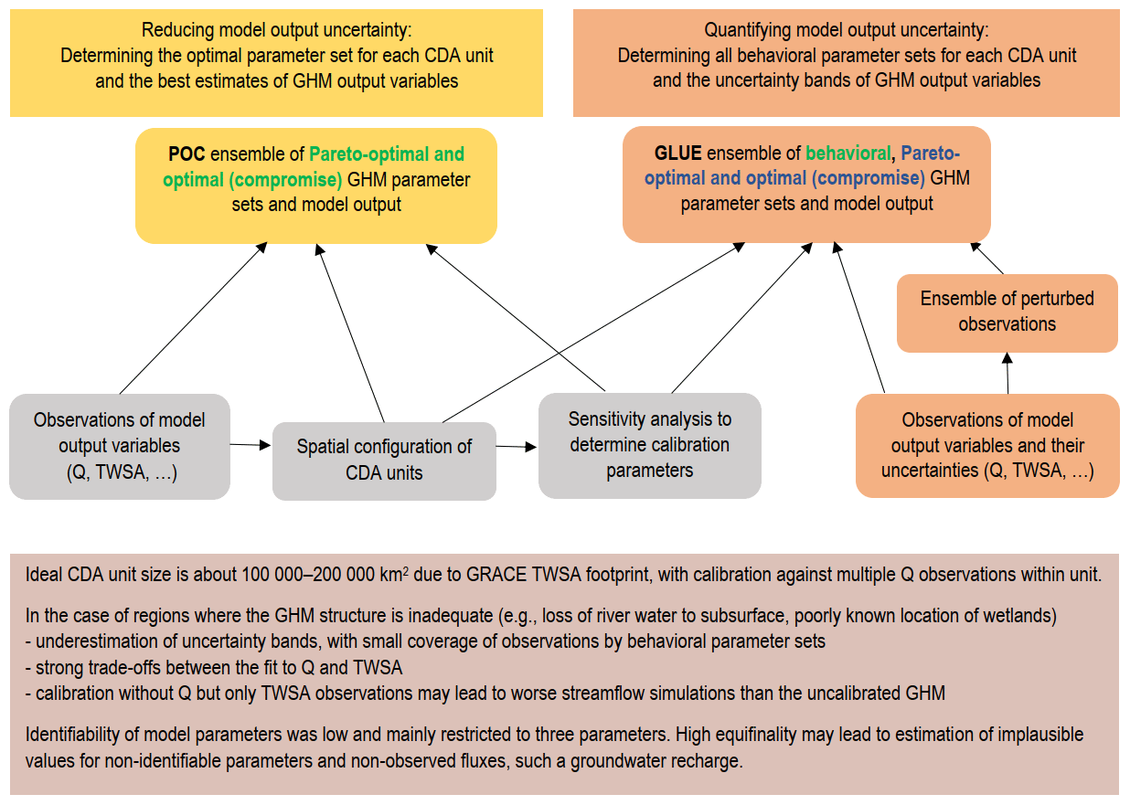
Figure 7The proposed approach for reducing and quantifying model output uncertainty of GHMs by multi-variable parameter estimation and the main recommendations and caveats for applying the approach in global hydrological modeling. Green letters indicate to which purpose POC and GLUE are best suited, while blue letters indicate an acceptable capability. A CDA unit is composed of all GHM grid cells to which the same calibration parameter value is assigned.
We conclude that a multi-variable POC approach that utilizes observations of both Q and TWSA, combined with the described sensitivity analysis, is best suited for estimating CDA-unit-specific Pareto-optimal parameter sets of GHMs (Fig. 7). The derived compromise parameter sets can then be used to simulate the best estimate of past and future water flows and storages – in particular, if various future scenarios, e.g., driven by the output of multiple climate models, or hydrological seasonal ensemble forecasts are computed by the GHMs. While the computational burden for a global-scale model calibration of, for example, 1000 basins is high, the run times are not prohibitive. However, in our study, multi-variable model calibration against both Q and TWSA constrained only three model parameters, while a large range of values of all other calibration parameters can lead to equally good fits to the observations, even if the uncertainty of observations is neglected. Therefore, any identified POC compromise parameter set should be applied with caution when estimating water flows, such as groundwater recharge, for which no observations were considered in the parameter estimation. We suggest that the parameter interdependence of Pareto-optimal parameter sets be analyzed.
This study has shown that, currently, among the three approaches used, only GLUE can be applied to quantify model output uncertainty caused by the observation uncertainties (Fig. 7). All behavioral parameter sets can be identified by applying the method for defining performance thresholds for behavioral parameter sets that we developed in this study, which uses both the GLUE ensemble and an ensemble of perturbed observations. As model performance with the optimal (compromise) parameter set as identified with GLUE is only slightly less than the performance with the optimal POC parameter set, GLUE can be used efficiently to compute both the best estimates and the uncertainty bounds of GHM model output. The computational efforts for calculating best estimates by POC and best estimates with uncertainty bounds by GLUE are similar. We found that the GLUE-derived model output uncertainty bands substantially underestimate the total model output uncertainty as they do not include the effects of model input and structure uncertainties.
We also conclude that the multi-variable EnCDA approach that we implemented in our pilot study is not yet competitive for GHM parameter estimation using Q and TWSA as (1) its performance (in terms of NSE) is lower during the calibration period than that of POC and GLUE or, for the large CDA unit of the MRB, even lower than that of the uncalibrated WaterGAP, and (2) its application during the validation period (without observational data) led to spurious results (Figs. 4 and S4). The intrinsic nonlinearity in simulating Q makes a multi-variable EnCDA that includes Q observations more difficult than an EnCDA that only includes TWSA or TWSA and other storage observations. In addition, the fact that the EnKF has to estimate many more state variables than model parameters means that the ensemble size will always be much more limited, and this hampers parameter calibration. We suggest that further research should investigate improved ensemble generation techniques for the case where the state vector is augmented by model parameters. Lastly, for model calibration purposes, one should investigate EnKF versions that optimize (weighted) MSE metrics in place of RMSE.
As we found that Q can be simulated reasonably well only at locations where Q observations have been used in the calibration but not upstream, the selection of rather small CDA units is advised. However, the CDA unit size cannot be smaller than approx. 100 000–200 000 km2 due to the large footprint of GRACE TWSA, and observations from more than one streamflow gauging station within the CDA unit might be utilized in parameter set optimization (Fig. 7). Additional observation variables such as snow cover and water storage variations in lakes and artificial reservoirs may be taken into account to further constrain parameter sets. Unfortunately, no information on groundwater level dynamics is available at the global scale, which is likely required to constrain the parameters related to surface water and groundwater abstraction (Hosseini-Moghari et al., 2020). Figure 7 lists further caveats for global-scale reduction and quantification of model output uncertainty by parameter estimation that were discussed in Sect. 5.
We recommend that, in the first step, GHMs are calibrated against observations of multiple variables, including Q and TWSA, by determining optimal calibration parameter sets for major basins with available Q observations as this is expected to improve the realism of the GHM output. To achieve this, an optimization algorithm similar to the one used for POC in this study should be applied. In the next step, a GLUE approach could be used to additionally estimate the model output uncertainty.
Climate change impact studies for individual river basins have shown that parameter sets with a similar performance during the calibration period may provide very different projections of climate change hazards and that the impact of parameter uncertainty can be similar to the impact of the selected climate or hydrological model selection (Mendoza et al., 2016; Her et al., 2019). Therefore, consideration of parameter uncertainty by running the hydrological model with several behavioral parameter sets helps to reduce the underestimation of the uncertainty of potential climate change impacts. However, producing a global-scale ensemble of potential future changes in hydrological variables by combining not only multiple greenhouse gas emissions scenarios, global climate models and global hydrological models (as is currently done in ISIMIP) but also model-specific behavioral parameter sets is currently infeasible. The main reason is that behavioral (or even optimal) parameter sets have not yet been determined for any global hydrological model in a spatially explicit manner at the global scale. In addition, the computational effort for such a multi-model and/or multi-parameter ensemble is likely to be prohibitive.
The POC, GLUE and EnCDA approaches share some characteristics and differ with regard to others (Table A1). All three start with a (large, in the case of POC and GLUE, and small, in the case of EnCDA) number of parameter sets that are derived from a priori assumptions about the probability distribution of calibration parameters and generate an ensemble of optimized parameter sets. EnCDA differs from POC and GLUE by simultaneously modifying model parameters and model states. EnCDA and GLUE are regarded to be Bayesian approaches as they aim to derive probability distributions of parameter sets and thus model output. In POC, the ensemble of Pareto-optimal parameter sets represents the uncertainty that is caused by the fact that, due to model structure and input uncertainty, different parameter sets lead to optimal performance for different calibration objectives. Information from observations is used in all three approaches to update an a priori belief about the probability distribution of parameters. However, parameter set selection is done in very different ways and is based on different assumptions. Both POC and GLUE compare the model output over the complete calibration period with all observations to determine performance metrics. While the evolutionary search algorithm of POC starts with a small number of parameter sets, runs the model and then generates new parameter sets with ever-improved performance metrics, in GLUE, the large initial ensemble generated from a priori parameter distributions is evaluated regarding performance metrics, and the behavioral members among the initial ensemble are identified. In POC and GLUE, parameters are temporally constant. In EnCDA, an ensemble of model runs is performed in a stepwise fashion from the time of one observation to the time of the next. EnCDA updates the parameters sequentially (in our study, each month) such that time series of recursive parameter estimates are computed. It is assumed that updates are informed by an ever-increasing amount of information from observations so that the parameter sets after the last update, i.e., at the end of the calibration period, are the best estimate. However, this can be disputed. A study on EnCDA using GRACE TWSA for the Australian Murray–Darling Basin showed that parameter values vary in time with changes in climatic conditions within the river basin, probably due to an inappropriate model structure that does not allow the correct translation of precipitation variability into model output variability (Schumacher et al., 2018). The capability to reveal such dynamics may be advantageous for improving our understanding of model deficiencies. It needs to be investigated whether and how EnCDA can be used to determine optimal parameter sets that are suitable for model runs without adjustment of states.
Table A1Comparison of the main characteristics of POC, GLUE and EnCDA as applied in this study.
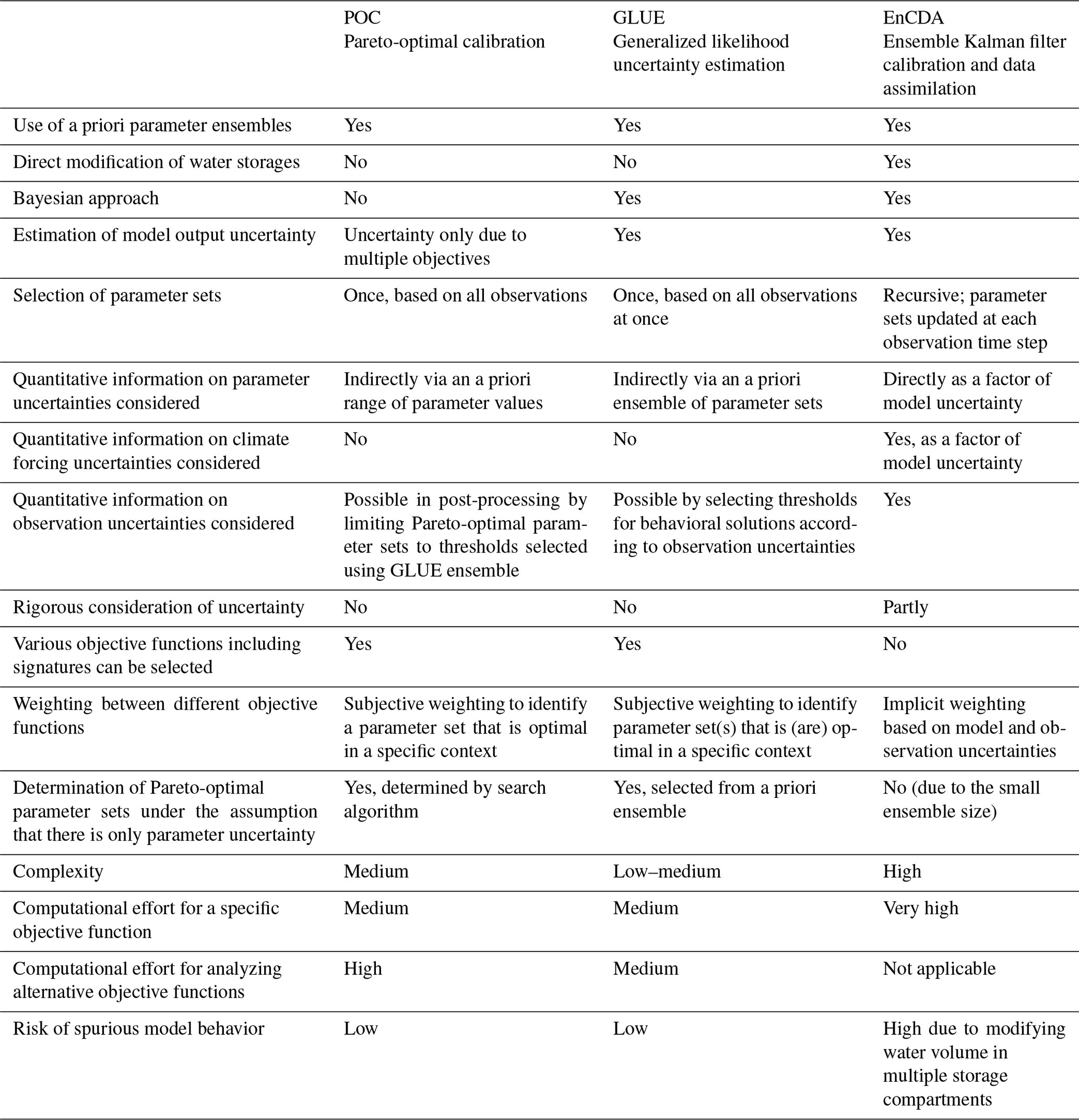
In EnCDA, quantified errors of both the model and the observations are required to update water storages and parameters in each of the ensemble members (Table A1). The ensemble serves to estimate the model error, which includes parameter and climate forcing uncertainty and is calculated as the variance of the differences between each ensemble member and the ensemble mean. The EnKF applied in EnCDA represents an optimal and unbiased estimator only under the assumption that errors are Gaussian, unbiased and well known, none of which is the case (Wang et al., 2020; Moradkhani et al., 2005; Beven and Binley, 1992). In GLUE, the model error due to parameter uncertainty (but not due to climate forcing uncertainty) is indirectly taken into account as the a priori ensemble depends on assumptions about parameter distribution, similarly to POC. Observation errors may be considered quantitatively, but, in most applications, they are not (Beven and Binley, 2014). In Sect. 3.4.2, we describe a way to take into account the observation uncertainties in GLUE. Werth and Güntner (2010) suggested a way to include observation errors in POC. First, they determined an error ellipse around the compromise solution (defined in Eq. 1) by first generating an ensemble of observations from perturbing the observation time series with the observation errors and then determining the range of performance values of the compromise solution for this ensemble of perturbed observations. By considering all the non-dominated and dominated parameter sets inside the error ellipse, they identified an ensemble of likely parameter sets that were informed by both observations and observation uncertainty. In this case, POC can, like EnCDA and GLUE, be used to estimate uncertainties of parameter sets and model outputs. Nevertheless, it should be noted that this approach does not incorporate observational uncertainty directly into multi-objective parameter calibration in a rigorous way. Therefore, we did not take this approach in our study.
Differently from EnCDA, with its rigorous handling of uncertainties, GLUE is an informal Bayesian approach that is much simpler than EnCDA (Table A1). Here, likelihood is understood in a very general sense as a fuzzy measure of the belief regarding how well the model conforms to the observed behavior of the system and not in the sense of maximum likelihood theory, which is the basis of EnCDA (Beven and Binley, 1992). In EnCDA, the likelihood of a parameter set is a product of model errors, observation errors, and the differences between observed and simulated variables (and other factors) (Sect. 3.2 in Schumacher, 2016). The informal and subjective treatment of uncertainty in the GLUE approach has caused controversy because the different error sources are not distinguished (Vrugt et al., 2009). This can mean that non-maximum likelihood solutions might be accepted as parameter estimates. However, the GLUE approach can be defended against formal Bayesian methods as these require a priori knowledge about errors that is lacking in most hydrological modeling applications (Beven and Binley, 2014). In addition, formal Bayesian methods (e.g., DREAM) are difficult to implement and much less computationally efficient but may lead to similar outcomes (Vrugt et al., 2009). In GLUE, the likelihood measure can be freely chosen by the modeler. One could choose a formal likelihood measure like the one applied for EnCDA, a measure that relates the deviation of model output from observations to the observation error or just any model performance metric for comparing observations to simulations (Beven and Binley, 2014, their Table 3). Given the large epistemic uncertainty about hydrological systems, GLUE relies on the subjective expertise of the modeler to define a suitable likelihood measure given the often only qualitative knowledge about uncertainties of model structure, model input, model parameters and observations. There is a multitude of likelihood measures that can be used to identify parameter sets that fit better to observations than the a priori ensemble (or the standard deterministic parameter set) and that are therefore more likely than others. A likelihood of zero is assigned to all parameter sets that are not behavioral, i.e., if the likelihood measure is below a threshold that is set subjectively by the modeler. For the example of the popular likelihood measure of the Nash–Sutcliffe efficiency (NSE), behavioral parameter sets may be defined as those that result in an NSE larger than 0.7 if the behavior of the hydrological system can be easily simulated; if not, the threshold will have to be lowered to obtain any behavioral parameter sets. To obtain the a posteriori probability distribution of parameter sets, only the behavioral parameter sets are considered, and their probability is derived from the NSE obtained with them.
Objective functions (i.e., likelihood measures and performance metrics) can be freely chosen in the case of POC and GLUE. This allows the selection of diverse hydrological signatures of the observables, e.g., those that focus on high or low flows in the case of streamflow. EnCDA minimizes the root mean squared error, and it is very difficult to apply another objective function (Table A1). In addition, the likelihood function in EnCDA considers only the deviations between the model output and observations at one point in time as the ensemble Kalman filter was applied in this study instead of the ensemble Kalman smoother. In contrast, performance measures used in POC and GLUE evaluate model performance (and calibrate model parameters) over the whole calibration period. EnCDA differs from POC and GLUE in that weighting between the performance metrics for the multiple objectives and/or variables is implicitly done given the model and observation errors (Table A1). In POC and GLUE, subjective weighting needs to be done for selecting one optimal parameter set. POC and GLUE also have in common the fact that they can serve to identify Pareto-optimal parameter sets or one compromise parameter set that can then be used in a computationally efficient way in model runs for climate change studies or seasonal forecasting, where hydrological models are driven by an ensemble of climate data sets.
The complexity of the three calibration approaches differs (Table A1). The computational burden is much higher for EnCDA than for POC and GLUE. Therefore, only a very small number of ensemble members can be used in the analysis; ensemble sizes are typically between 30 and 100. These low-rank ensembles may fail to correctly convey the covariance information between model states and parameters or between different parameters. Localization techniques can be applied to mitigate this effect but with the trade-off that long-distance covariance information is neglected or down-weighted. For the same number of evaluated parameter sets, the computational effort of POC and GLUE is approximately the same for evaluating a specific objective function. However, as the parameter ensemble generated by the search algorithm in POC depends on the objective function (unlike in the case of GLUE), the computational burden of POC becomes, for example, twice as high as that of GLUE if one alternative objective function is taken into account. Finally, EnCDA is prone to spurious results as the modification of water storages to improve the fit to TWSA observations might lead to little-constrained changes in individual storages, with impacts on simulated water flows. In the EnCDA study of Schumacher et al. (2018), river storage was adjusted in WaterGAP based on TWSA observations, leading to spurious increases in Q not seen in WaterGAP runs without water storage updates or in the observations.
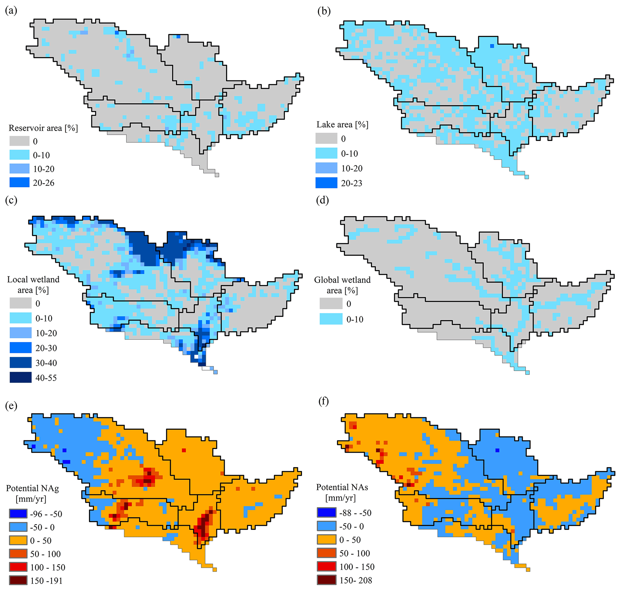
Figure B1Artificial reservoirs (a), lakes (b), local wetlands (c), global wetlands (d), and potential net abstractions from groundwater (e) and from surface water (f) in the CDA units of the MRB, as taken into account in WaterGAP. Maximum areal extents of the surface bodies in percentages of the 0.5° cell area are shown, while potential net abstractions (in mm yr−1) are provided for the period 2003–2012.
To understand the sensitivity of model output to parameters, the spatial distribution of the storages and flows that they affect is required. Water balances of reservoirs (Fig. B1a) are not directly impacted by the calibration parameters in Table 1, while lake dynamics (Fig. B1b) are directly impacted by active lake depth (SW-LD), and wetlands (Fig. B1c, d) are directly impacted by active wetland depth (SW-WD). Please note that knowledge about the wetlands in the northern parts of the CDA units of the Missouri River basin and the upper MRB, as well as in the southern part of the lower MRB, is restricted to the information that, generally, in these areas, 25 %–50 % of the land area is covered by wetlands in the wet season. In WaterGAP, this information was translated into a maximum extent of local wetlands of 35 %. The surface water discharge coefficient (SW-DC) affects both lakes and wetlands. Potential net abstractions from groundwater (Fig. B1e) and surface water (Fig. B1f) are simulated with a monthly time step for each grid cell, and multipliers for each of them (NA-GM and NA-SM) affect model output differently in the various CDA units due to different net abstraction patterns.
Table C1KGE components of model runs of Table 2 regarding Q for the calibration period 2003–2012.
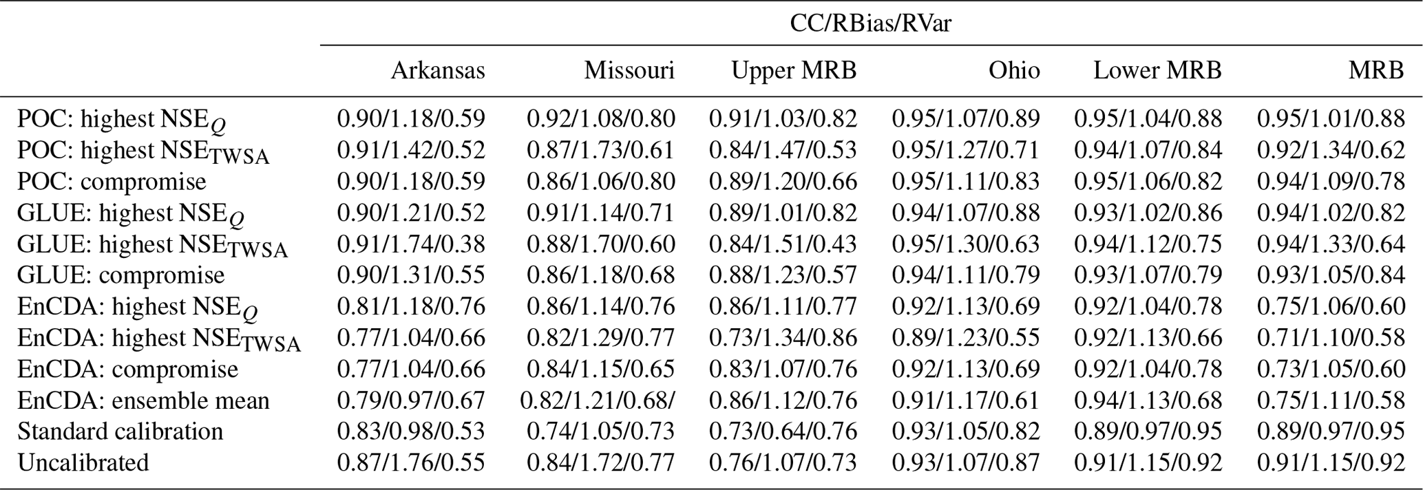
Table C2KGE components of model runs of Table 2 regarding TWSA for the calibration period 2003–2012.
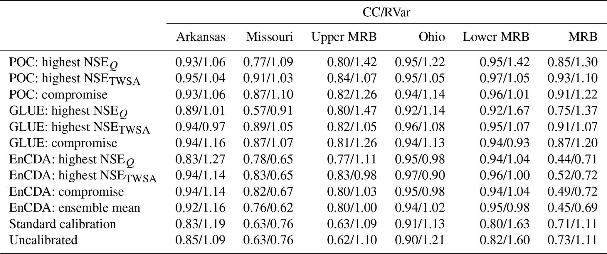
The WaterGAP 2.2d code is accessible at https://doi.org/10.5281/zenodo.6902110 (Müller Schmied et al., 2023).
Level-2 GRACE data (spherical harmonic coefficients) used to compute observed TWSA are available from https://doi.org/10.5880/ICGEM.2018.003 (Mayer-Gürr et al., 2018). All optimal and behavioral parameter sets obtained by the three calibration approaches for the six CDA units, together with the resulting performance metrics, are listed in an Excel file that is part of the Supplement.
The supplement related to this article is available online at: https://doi.org/10.5194/hess-28-2259-2024-supplement.
PD designed the study, with contributions from HMMH, KS, SMHM, SS, AG and JK. HMMH, KS and HG performed the calibration and data analyses. HMMH and SMHM produced the figures. SA and HMS improved the WaterGAP code. LB and HG processed and analyzed GRACE TWSA data. PD wrote the original draft of the paper. All the authors contributed to the final draft.
The contact author has declared that none of the authors has any competing interests.
Publisher’s note: Copernicus Publications remains neutral with regard to jurisdictional claims made in the text, published maps, institutional affiliations, or any other geographical representation in this paper. While Copernicus Publications makes every effort to include appropriate place names, the final responsibility lies with the authors.
The authors thank Olga Sydak (née Engels) for the first analyses and discussions, Christoph Niemann for contributing to the generation of figures, and three reviewers and the editor for the valuable comments and suggestions that helped to improve the paper.
This research has been supported by the Deutsche Forschungsgemeinschaft (DFG research unit “Understanding the global freshwater system by combining geodetic and remote sensing information with modelling using a calibration/data assimilation approach (GlobalCDA)”.).
This open-access publication was funded by Goethe University Frankfurt.
This paper was edited by Adriaan J. (Ryan) Teuling and reviewed by three anonymous referees.
Alcamo, J., Döll, P., Henrichs, T., Kaspar, F., Lehner, B., Rösch, T., and Siebert, S.: Development and testing of the WaterGAP 2 global model of water use and availability, Hydrolog. Sci. J., 48, 317–338, https://doi.org/10.1623/hysj.48.3.317.45290, 2003.
Beven, K.: Prophecy, reality and uncertainty in distributed hydrological modeling, Adv. Water Resour., 16, 41–51, https://doi.org/10.1016/0309-1708(93)90028-E, 1993.
Beven, K.: Towards an alternative blueprint for a physically based digitally simulated hydrologic response modelling system, Hydrol. Process., 16, 189–206, https://doi.org/10.1002/hyp.343, 2002.
Beven, K. and Binley, A.: The future of distributed models: model calibration and uncertainty prediction, Hydrol. Process., 6, 279–298, https://doi.org/10.1002/hyp.3360060305, 1992.
Beven, K. and Binley, A.: GLUE. 20 years on, Hydrol. Process., 28, 5897–5918, https://doi.org/10.1002/hyp.10082, 2014.
Beven, K. and Smith, P.: Concepts of information content and likelihood in parameter calibration for hydrological simulation models, J. Hydrol. Eng., 20, A4014010, https://doi.org/10.1061/(ASCE)HE.1943-5584.0000991, 2015.
Bierkens, M. F. P.: Global hydrology 2015. State, trends, and directions, Water Resour. Res., 51, 4923–4947, https://doi.org/10.1002/2015WR017173, 2015.
Blasone, R.-S., Vrugt, J. A., Madsen, H., Rosbjerg, D., Robinson, B. A., and Zyvoloski, G. A.: Generalized likelihood uncertainty estimation (GLUE) using adaptive Markov chain Monte Carlo sampling, Adv. Water Resour., 31, 630–648, https://doi.org/10.1016/j.advwatres.2007.12.003, 2008
Blazkova, S. and Beven, K.: A limits of acceptability approach to model evaluation and uncertainty estimation in flood frequency estimation by continuous simulation: Skalka catchment, Czech Republic, Water Resour. Res., 45, W00B16, https://doi.org/10.1029/2007WR006726, 2009.
Campolongo, F., Saltelli, A., and Cariboni, J.: From screening to quantitative sensitivity analysis. A unified approach, Comput. Phys. Commun., 182, 978–988, https://doi.org/10.1016/j.cpc.2010.12.039, 2011.
Clark, M., Rupp, D., Woods, R., Zheng, X., Ibbitt, R., and Slater, A.: Hydrological data assimilation with the ensemble Kalman filter. Use of streamflow observations to update states in a distributed hydrological model, Adv. Water Resour., 31, 1309–1324, https://doi.org/10.1016/j.advwatres.2008.06.005, 2008.
Dembélé, M., Hrachowitz, M., Savenije, H. H. G., Mariéthoz, G., and Schaefli, B.: Improving the predictive skill of a distributed hydrological model by calibration on spatial patterns with multiple satellite data sets, Water Resour. Res., 56, e2019WR026085, https://doi.org/10.1029/2019WR026085, 2020.
Di Baldassarre, G. and Montanari, A.: Uncertainty in river discharge observations: a quantitative analysis, Hydrol. Earth Syst. Sci., 13, 913–921, https://doi.org/10.5194/hess-13-913-2009, 2009.
Döll, P., Kaspar, F., and Lehner, B.: A global hydrological model for deriving water availability indicators: model tuning and validation, J. Hydrol., 270, 105–134, https://doi.org/10.1016/S0022-1694(02)00283-4, 2003.
Döll, P., Fritsche, M., Eicker, A., and Müller Schmied, H.: Seasonal Water Storage Variations as Impacted by Water Abstractions: Comparing the Output of a Global Hydrological Model with GRACE and GPS Observations, Surv. Geophys., 35, 1311–1331, https://doi.org/10.1007/s10712-014-9282-2, 2014.
Döll, P., Douville, H., Güntner, A., Müller Schmied, H., and Wada, Y.: Modelling freshwater resources at the global scale: Challenges and prospects, Surv. Geophys., 37, 195–221, https://doi.org/10.1007/s10712-015-9343-1, 2016.
Döll, P., Trautmann, T., Göllner, M., and Müller Schmied, H.: A global-scale analysis of water storage dynamics of inland wetlands: Quantifying the impacts of human water use and man-made reservoirs as well as the unavoidable and avoidable impacts of climate change, Ecohydrology, 13, e2175, https://doi.org/10.1002/eco.2175, 2020.
Efstratiadis, A. and Koutsoyiannis, D.: One decade of multi-objective calibration approaches in hydrological modelling: a review, Hydrolog. Sci. J., 55, 58–78, https://doi.org/10.1080/02626660903526292, 2010.
Eicker, A., Schumacher, M., Kusche, J., Döll, P., and Müller Schmied, H.: Calibration/Data Assimilation Approach for Integrating GRACE Data into the WaterGAP Global Hydrology Model (WGHM) Using an Ensemble Kalman Filter: First Results, Surv. Geophys., 35, 1285–1309, https://doi.org/10.1007/s10712-014-9309-8, 2014.
Evensen, G.: Sequential data assimilation with a nonlinear quasi-geostrophic model using Monte Carlo methods to forecast error statistics, J. Geophys. Res.-Oceans, 99, 10143–10162, 1994.
Evensen, G.: The ensemble Kalman filter: Theoretical formulation and practical implementation, Ocean Dynam., 53, 343–367, https://doi.org/10.1007/s10236-003-0036-9, 2003.
Gerdener, H., Engels, O., and Kusche, J.: A framework for deriving drought indicators from the Gravity Recovery and Climate Experiment (GRACE), Hydrol. Earth Syst. Sci., 24, 227–248, https://doi.org/10.5194/hess-24-227-2020, 2020.
Gerdener, H., Kusche, J., Schulze, K., Döll, P., and Klos, A.: The global land water storage data set release 2 (GLWS2.0) derived via assimilating GRACE and GRACE-FO data into a global hydrological model, J. Geodesy, 97, 73, https://doi.org/10.1007/s00190-023-01763-9, 2023.
Girotto, M., de Lannoy, G. J. M., Reichle, R. H., and Rodell, M.: Assimilation of gridded terrestrial water storage observations from GRACE into a land surface model, Water Resour. Res., 52, 4164–4183, https://doi.org/10.1002/2015WR018417, 2016.
Gupta, H. V., Sorooshian, S., and Ogou Yapo, P.: Toward improved calibration of hydrologic models: Multiple and noncommensurable measures of information, Water Resour. Res., 34, 751–763, https://doi.org/10.1029/97WR03495, 1998.
Hadka, D. and Reed, P.: Borg: An Auto-Adaptive Many-Objective Evolutionary Computing Framework, Evol. Comput., 21, 231–259, https://doi.org/10.1162/EVCO_a_00075, 2013.
Harlin, J. and Kung, C.-S.: Parameter uncertainty and simulation of design floods in Sweden, J. Hydrol., 137, 209–230, https://doi.org/10.1016/0022-1694(92)90057-3, 1992.
Her, Y., Yoo, S.-H., Cho, J., Hwang, S., Jeong, J., and Seong, C.: Uncertainty in hydrological analysis of climate change: multi-parameter vs. multi-GCM ensemble predictions, Sci. Rep., 9, 4974, https://doi.org/10.1038/s41598-019-41334-7, 2019.
Hosseini-Moghari, S.-M., Araghinejad, S., Tourian, M. J., Ebrahimi, K., and Döll, P.: Quantifying the impacts of human water use and climate variations on recent drying of Lake Urmia basin: the value of different sets of spaceborne and in situ data for calibrating a global hydrological model, Hydrol. Earth Syst. Sci., 24, 1939–1956, https://doi.org/10.5194/hess-24-1939-2020, 2020.
Hunger, M. and Döll, P.: Value of river discharge data for global-scale hydrological modeling, Hydrol. Earth Syst. Sci., 12, 841–861, https://doi.org/10.5194/hess-12-841-2008, 2008.
Jasechko, S., Seybold, H., Perrone, D., Fan, Y., and Kirchner, J. W.: Widespread potential loss of streamflow into underlying aquifers across the USA, Nature, 591, 391–397, https://doi.org/10.1038/s41586-021-03311-x, 2021.
Jin, X., Xu, C.-Y., Zhang, Q., and Singh, V. P.: Parameter and modeling uncertainty simulated by GLUE and a formal Bayesian method for a conceptual hydrological model, J. Hydrol., 383, 147–155, https://doi.org/10.1016/j.jhydrol.2009.12.028, 2010.
Jost, G., Moore, R. D., Menounos, B., and Wheate, R.: Quantifying the contribution of glacier runoff to streamflow in the upper Columbia River Basin, Canada, Hydrol. Earth Syst. Sci., 16, 849–860, https://doi.org/10.5194/hess-16-849-2012, 2012.
Khu, S. T. and Madsen, H.: Multiobjective calibration with Pareto preference ordering: An application to rainfall-runoff model calibration, Water Resour. Res., 41, W03004, https://doi.org/10.1029/2004WR003041, 2005.
Kling, H., Fuchs, M., and Paulin, M.: Runoff conditions in the upper Danube basin under an ensemble of climate change scenarios, J. Hydrol., 424–425, 264–277, https://doi.org/10.1016/j.jhydrol.2012.01.011, 2012.
Kumar, S. V., Zaitchik, B. F., Peters-Lidard, C. D., Rodell, M., Reichle, R., Li, B., Jasinski, M., Mocko, D., Getirana, D., De Lannoy, G., Cosh, M. H., Hain, C. R., Anderson, M., Arsenault, K. R., Xia, Y., and Ek, M.: Assimilation of gridded GRACE terrestrial water storage estimates in the North American Land Data Assimilation System, J. Hydrometeorol., 17, 1951–1972, https://doi.org/10.1175/JHM-D-15-0157.1, 2016.
Kupzig, J., Reinecke, R., Pianosi, F., Flörke, M., and Wagener, T.: Towards parameter estimation in global hydrological models, Environ. Res. Lett., 18, 074023, https://doi.org/10.1088/1748-9326/acdae8, 2023.
Kusche, J., Schmidt, R., Petrovic, S., and Rietbroek, R.: Decorrelated GRACE time-variable gravity solutions by GFZ, and their validation using a hydrological model, J. Geodesy, 83, 903–913, https://doi.org/10.1007/s00190-009-0308-3, 2009.
Lehner, B. and Döll, P.: Development and validation of a global database of lakes, reservoirs and wetlands, J. Hydrol., 296, 1–22, https://doi.org/10.1016/j.jhydrol.2004.03.028, 2004.
Longuevergne, L., Scanlon, B. R., and Wilson, C. R.: GRACE hydrological estimates for small basins: Evaluating processing approaches on the High Plains Aquifer, USA, Water Resour. Res., 46, W11517, https://doi.org/10.1029/2009wr008564, 2010.
Mayer-Gürr, T., Behzadpur, S., Ellmer, M., Kvas, A., Klinger, B., Strasser, S., and Zehentner, N.: ITSG-Grace2018 – Monthly, Daily and Static Gravity Field Solutions from GRACE, GFZ Data Services [data set], https://doi.org/10.5880/ICGEM.2018.003, 2018.
McMillan, H., Krueger, T., and Freer, J.: Benchmarking observational uncertainties for hydrology. Rainfall, river discharge and water quality, Hydrol. Process., 26, 4078–4111, https://doi.org/10.1002/hyp.9384, 2012.
Mendoza, P. A., Clark, M. P, Mizukami, N., Gutmann, E. D., Arnold, J. R., Brekke, L. D., and Rajagopalan, B.: How do hydrologic modeling decisions affect the portrayal of climate change impacts?, Hydrol. Process., 30, 1071–1095, https://doi.org/10.1002/hyp.10684, 2016.
Minke, A. G., Westbrook, C. J., and van der Kamp, G.: Simplified volume-area-depth method for estimating water storage of Prairie potholes, Wetlands, 30, 541–551, http;//doi.org/ 10.1007/s13157-010-0044-8, 2010.
Mizukami, N., Clark, M. P., Newman, A. J., Wood, A. W., Gutmann, E. D., and Nijssen, B.: Towards seamless large-domain parameter estimation for hydrologic models, Water Resour. Res., 53, 8020–8040, https://doi.org/10.1002/2017WR020401, 2017.
Moradkhani, H., Hsu, K.-L., Gupta, H., and Sorooshian, S.: Uncertainty assessment of hydrologic model states and parameters: Sequential data assimilation using the particle filter, Water Resour. Res., 41, W05012, https://doi.org/10.1029/2004WR003604, 2005.
Morris, M. D.: Factorial sampling plans for preliminary computational experiments, Technometrics, 33, 161–174, https://doi.org/10.1080/00401706.1991.10484804, 1991.
Müller Schmied, H., Eisner, S., Franz, D., Wattenbach, M., Portmann, F. T., Flörke, M., and Döll, P.: Sensitivity of simulated global-scale freshwater fluxes and storages to input data, hydrological model structure, human water use and calibration, Hydrol. Earth Syst. Sci., 18, 3511–3538, https://doi.org/10.5194/hess-18-3511-2014, 2014.
Müller Schmied, H., Cáceres, D., Eisner, S., Flörke, M., Herbert, C., Niemann, C., Peiris, T. A., Popat, E., Portmann, F. T., Reinecke, R., Schumacher, M., Shadkam, S., Telteu, C.-E., Trautmann, T., and Döll, P.: The global water resources and use model WaterGAP v2.2d: model description and evaluation, Geosci. Model Dev., 14, 1037–1079, https://doi.org/10.5194/gmd-14-1037-2021, 2021.
Müller Schmied, H., Trautmann, T., Ackermann, S., Cáceres, D., Flörke, M., Gerdener, H., Kynast, E., Peiris, T. A., Schiebener, L., Schumacher, M., and Döll, P.: WaterGAP v2.2e, Zenodo [code], https://doi.org/10.5281/zenodo.6902110, 2023.
Nerger, L. and Hiller, W.: Software for ensemble-based data assimilation systems – Implementation strategies and scalability, Comput. Geosci., 55, 110–118, https://doi.org/10.1016/j.cageo.2012.03.026, 2013.
Paiva, R. C. D., Collischonn, W., Bonnet, M.-P., de Gonçalves, L. G. G., Calmant, S., Getirana, A., and Santos da Silva, J.: Assimilating in situ and radar altimetry data into a large-scale hydrologic-hydrodynamic model for streamflow forecast in the Amazon, Hydrol. Earth Syst. Sci., 17, 2929–2946, https://doi.org/10.5194/hess-17-2929-2013, 2013.
Pianosi, F. Beven, K., Freer, J., Hall, J. W., Rougier, J. Stephenson, D. B., and Wagener, T.: Sensitivity analysis of environmental models: A systematic review with practical workflow, Environ. Modell. Softw., 79, 214–232, https://doi.org/10.1016/j.envsoft.2016.02.008, 2016.
Rakovec, O., Kumar, R., Attinger, S., and Samaniego, L.: Improving the realism of hydrologic model functioning through multivariate parameter estimation, Water Resour. Res., 52, 7779–7792, https://doi.org/10.1002/2016WR019430, 2016.
Scanlon, B. R., Zhang, Z., Save, H., Sun, A. Y., Müller Schmied, H., and van Beek, L. P. H.: Global models underestimate large decadal declining and rising water storage trends relative to GRACE satellite data, P. Natl. Acad. Sci. USA, 115, E1080–E1089, https://doi.org/10.1073/pnas.1704665115, 2018.
Scanlon, B. R., Zhang, Z., Rateb, A., Sun, A., Wiese, D., and Save, H.: Tracking Seasonal Fluctuations in Land Water Storage Using Global Models and GRACE Satellites, Geophys. Res. Lett., 46, 5254–5264, https://doi.org/10.1029/2018GL081836, 2019.
Schumacher, M.: Methods for Assimilating Remotely-Sensed Water Storage Changes into Hydrological Models, PhD thesis, University of Bonn, Bonn, https://hdl.handle.net/20.500.11811/6630 (last access: 22 May 2024), 2016.
Schumacher, M., Kusche, J., and Döll, P.: A systematic impact assessment of GRACE error correlation on data assimilation in hydrological models, J. Geodesy, 90, 537–559, https://doi.org/10.1007/s00190-016-0892-y, 2016a.
Schumacher, M., Eicker, A., Kusche, J., Müller Schmied, H., and Döll, P.: Covariance Analysis and Sensitivity Studies for GRACE Assimilation into WGHM, in: IAG 150 Years, edited by: Rizos, C. and Willis, P., Proceedings of the IAG Scientific Assembly in Postdam, Germany, 2013, Vol. 143, 1st edn., Cham, s.l.: Springer International Publishing International Association of Geodesy Symposia, Vol. 143, 241–247, https://doi.org/10.1007/1345_2015_119, 2016b.
Schumacher, M., Forootan, E., van Dijk, A.I.J.M., Müller Schmied, H., Crosbie, R. S., Kusche, J., and Döll, P.: Improving drought simulations within the Murray-Darling basin by combined calibration/assimilation of GRACE data into the WaterGAP Global Hydrology Model, Remote Sens. Environ., 204, 212–228, https://doi.org/10.1016/j.rse.2017.10.029, 2018.
Stisen, S., Koch, J., Sonnenborg, T. O., Refsgaard, J. C., Bircher, S., Ringgaard, R., and Jensen, K. H.: Moving beyond run-off calibration – Multivariable optimization of a surface-subsurface-atmosphere model, Hydrol. Process., 32, 2654–2668, https://doi.org/10.1002/hyp.13177, 2018.
Troy, T. J., Wood, E. F., and Sheffield, J.: An efficient calibration method for continental-scale land surface modeling, Water Resour. Res., 44, W09411, https://doi.org/10.1029/2007WR006513, 2008.
Vishwakarma, B. D., Zhang, J., and Sneeuw, N.: Downscaling GRACE total water storage change using partial least squares regression, Sci. Data, 8, 95, https://doi.org/10.1038/s41597-021-00862-6, 2021.
Vrugt, J. A., ter Braak, C. J. F., Gupta, H. V., and Robinson, B. A.: Equifinality of formal (DREAM) and informal (GLUE) Bayesian approaches in hydrologic modeling?, Stoch Env. Res. Risk A., 23, 1011–1026, https://doi.org/10.1007/s00477-008-0274-y, 2009.
Wanders, N., Bierkens, M. F. P., de Jong, S. M., Roo, A., and Karssenberg, D.: The benefits of using remotely sensed soil moisture in parameter identification of large-scale hydrological models, Water Resour. Res., 50, 6874–6891, https://doi.org/10.1002/2013WR014639, 2014.
Wang, Q. J., Bennett, J. C., Robertson, D. E., and Li, M.: A data censoring approach for predictive error modelling of flow in ephemeral rivers, Water Resour. Res., 56, e2019WR026128, https://doi.org/10.1029/2019WR026128, 2020.
Weedon, G. P., Balsamo, G., Bellouin, N., Gomes, S., Best, M. J., and Viterbo, P.: The WFDEI meteorological forcing data set: WATCH Forcing Data methodology applied to ERA-Interim reanalysis data, Water Resour. Res., 50, 7505–7514, https://doi.org/10.1002/2014WR015638, 2014.
Werth, S. and Güntner, A.: Calibration analysis for water storage variability of the global hydrological model WGHM, Hydrol. Earth Syst. Sci., 14, 59–78, https://doi.org/10.5194/hess-14-59-2010, 2010.
Westerberg, I. K., Wagener, T., Coxon, G., McMillan, H. K., Castellarin, A., Montanari, A., and Freer, J.: Uncertainty in hydrological signatures for gauged and ungauged catchments, Water Resour. Res., 52, 1847–1865, https://doi.org/10.1002/2015WR017635, 2016.
Xie, H., Longuevergne, L., Ringler, C., and Scanlon, B. R.: Calibration and evaluation of a semi-distributed watershed model of Sub-Saharan Africa using GRACE data, Hydrol. Earth Syst. Sci., 16, 3083–3099, https://doi.org/10.5194/hess-16-3083-2012, 2012.
Xie, X. and Zhang, D.: A partitioned update scheme for state-parameter estimation of distributed hydrologic models based on the ensemble Kalman filter, Water Resour. Res., 49, 7350–7365, https://doi.org/10.1002/2012WR012853, 2013.
Yassin, F., Rzavi, S., Wheater, H., Sapriza-Azuri, G., Davison, B., and Pietroniro, A.: Enhanced identification of a hydrologic model using streamflow and satellite water storage data: A multicriteria sensitivity analysis and optimization approach, Hydrol. Process., 31, 3320–3333, https://doi.org/10.1002/hyp.11267, 2017.
Yu, P. L.: A class of solutions for group decision problems, Manage. Sci., 19, 936–946, https://doi.org/10.1287/mnsc.19.8.936, 1973.
Zaitchik, B. F., Rodell, M., and Reichle, R. H.: Assimilation of GRACE Terrestrial Water Storage Data into a Land Surface Model: Results for the Mississippi River Basin, J. Hydrometeor., 9, 535–548, https://doi.org/10.1175/2007JHM951.1, 2008.
- Abstract
- Introduction
- Approaches for parameter and uncertainty estimation in global hydrological modeling based on observations of multiple model output variables
- Methods and data
- Results
- Discussion
- Conclusions
- Appendix A: Comparison of the three ensemble-based approaches
- Appendix B: Surface waterbodies and human water abstractions in the CDA units of the Mississippi River basin
- Appendix C: Performance of different calibration methods during the calibration period 2003–2012: components of the KGE performance metric for both Q and TWSA
- Code availability
- Data availability
- Author contributions
- Competing interests
- Disclaimer
- Acknowledgements
- Financial support
- Review statement
- References
- Supplement