Assessing decadal- to centennial-scale nonstationary variability in meteorological drought trends

There are indications that the reference climatology underlying meteorological drought has shown nonstationarity at seasonal, decadal, and centennial timescales, impacting the calculation of drought indices and potentially having ecological and economic consequences. Analyzing these trends in meteorological drought climatology beyond 100 years, a time frame which exceeds the available period of observation data, contributes to a better understanding of the nonstationary changes, ultimately determining whether they are within the range of natural variability or outside this range. To accomplish this, our study introduces a novel approach to integrate unevenly scaled tree-ring proxy data from the North American Seasonal Precipitation Atlas (NASPA) with instrumental precipitation datasets by first temporally downscaling the proxy data to produce a regular time series and then modeling climate nonstationarity while simultaneously correcting model-induced bias. This new modeling approach was applied to 14 sites across the continental United States using the 3-month standardized precipitation index (SPI) as a basis. The findings showed that certain locations have experienced recent rapid shifts towards drier or wetter conditions during the instrumental period compared to the past 1000 years, with drying trends generally found in the west and wetting trends in the east. This study also found that seasonal shifts have occurred in some regions recently, with seasonality changes most notable for southern gauges. We expect that our new approach provides a foundation for incorporating various datasets to examine nonstationary variability in long-term precipitation climatology and to confirm the spatial patterns noted here in greater detail.

1 Introduction

Understanding meteorological drought trends is important as the entangled impacts of anthropogenic climate change and natural climate variability have shown complicated patterns of precipitation change over the last century (Ault, 2020; Schubert et al., 2016). Drought severity and duration have changed over time at seasonal, interannual, or centennial scales, with subsequent impacts on human and ecological systems (Trenberth, 2011; Van Loon et al., 2016). Many studies have investigated trends or shifts in drought related to climate change (Marvel et al., 2021; Williams et al., 2020; Mishra et al., 2010; Marvel et al., 2019; Trenberth et al., 2014). Previous research has relied heavily on observed or remotely sensed precipitation records, which often do not cover periods exceeding 100 years. Although such observations can capture modern drought trends, 100 years of data are not sufficient for determining whether recent drought trends are part of long-term cyclic variability, due to recent unprecedented trends, or are a combination of the two (Easterling et al., 2000; Cook et al., 2015).

In addition, previous studies have indicated that precipitation seasonality has changed during the observed period. These changes include increases in the amplitude between the wet and dry seasons or temporal shifts in the driest/wettest period (Marvel et al., 2021; Weiss et al., 2009; Pal et al., 2013). Even without substantial changes in the annual mean precipitation, shifts in precipitation seasonality can have a significant impact on local ecosystems or anthropogenic water management schemes, such as reservoirs, that rely on storing and releasing seasonal flow. As a result, understanding seasonal cycles and nonstationary shifts in seasonality is important for building adaptive and robust water management schemes (Konapala et al., 2020). For climate projections over the next 100 years, Marvel et al. (2021) found projected changes in annual precipitation cycles across the US Midwest and the upper Great Plains. This region is projected to undergo a shift in peak precipitation to earlier in the year without substantial changes in precipitation. This study also projected an increase in precipitation during the wettest season (winter) in the Northwest and Southeast US, thereby increasing the seasonal variance in precipitation. Changes in seasonality or seasonal variance can be better understood when viewed in a historical context using a much longer time window to determine whether they are within the range of natural climate variability or outside this range (Coats et al., 2015).

Therefore, much longer timescales are needed for a comprehensive understanding of nonstationary drought trends, preferably using a multi-centennial timescale (Torbenson and Stahle, 2018; Herweijer et al., 2007; Cook et al., 2010a; Diffenbaugh et al., 2015). Paleoclimate reconstructions use environmental proxies, such as tree-ring chronologies or speleothem records that physically record some aspect of climate, and can cover a much longer period than instrumental observations (Cook et al., 2016). For example, this study uses a reconstruction of precipitation across North America based on tree rings, which infer the relative availability of regional precipitation or soil moisture from the annual growth. This particular reconstruction is a continental-scale gridded reconstruction rather than a regional or local gridded reconstruction. Large-scale gridded reconstructions sacrifice some local precision but have the benefit of generating a single complete dataset based on a common methodology, which can leverage a larger catalog of chronologies. Several such gridded hydrometeorological reconstruction datasets using tree-ring proxies are available across North America. The North American Drought Atlas (NADA; Cook et al., 1999) reconstructs the Palmer drought severity index (PDSI; Palmer, 1965) for June–August (JJA) from 0–2006 CE (hereafter all years are denoted in CE) and has been used to determine historic drought severities (Cook et al., 2010b; Cook and Krusic, 2008). The North American Seasonal Precipitation Atlas (NASPA) is another precipitation reconstruction recently developed with two distinct seasons: December–April (DJFMA) and May–July (MJJ) (Stahle et al., 2020a). The NASPA dataset provides both the standardized precipitation index (SPI) and averaged precipitation for both the cool and warm seasons. The NASPA is used here since it covers the past 2000 years and contains cool- and warm-season records for each year. Over 2000 years of subannual-scale records enable an investigation of nonstationary drought trends and seasonal shifts at a multi-centennial scale if they can be combined with recently observed instrumental datasets (Trenberth et al., 2014; Marvel et al., 2019; Cook et al., 2016).

Despite the value of long reconstructions, comparing meteorological drought trends across observed and proxy-based reconstruction datasets is challenging as these data types are often not directly compatible (Baek et al., 2017; St. George et al., 2010). The first challenge is that each dataset often has non-negligible biases. Biases in proxy reconstructions can be caused by indirect measurement of the target variable, e.g., precipitation, by means of tree-ring growth. For example, bias can be introduced during the standardization process, which is designed to isolate the interannual signal from the long-term geometric growth of a tree. Trees also have physiological responses to continuous extreme drought or pluvials, which can limit variance at the extremes (Franke et al., 2013; Robeson et al., 2020). Even among gridded datasets based on gauge observations, bias can be introduced by the use of imperfect transforming algorithms (Sun et al., 2018) due to orographic-induced bias, underestimation of trace precipitation amounts (Goodison et al., 1998), or wind-related undercatch (Pollock et al., 2018). Thereby, precipitation measurements for the same period can differ across datasets. These biases can cause one dataset to systematically under- or overestimate precipitation compared to other datasets (Robeson et al., 2020) or modify the range of estimates. Quantifying and minimizing these biases is necessary to merge disparate datasets and analyze a common trend across various datasets.

A second challenge for merging reconstructions with observations concerns their heterogeneous spatial and temporal scales (Cook and Krusic, 2008). For example, the NASPA reconstructions provide only two time series per year with different precipitation periods: May–July and December–April. Instrumental datasets can have subdaily, daily, or monthly temporal scales (Howard et al., 2021). Therefore, timescales must be unified if one is to merge instrumental with reconstructed datasets to observe common nonstationary seasonal trends. In addition, the spatial resolution of gridded datasets varies, and centers of those grid cells do not always match. Thus, matching co-located grid cells through creating a common spatial resolution is an important aspect of representing common characteristics in precipitation (Abatzoglou, 2013).

This study is designed to address the challenge of constructing 2000 years of precipitation climatology by merging multiple datasets with varied biases and temporal scales. The objectives of this study are therefore to (1) construct downscaled NASPA precipitation time series (downscaling from a biannual to a monthly scale) with a 3-month average resolution, (2) identify unique biases inherent in different precipitation data and remove these biases, and ultimately (3) construct a 2000-year continuous climatology model that can capture century-scale shifts in 3-month average precipitation. This approach mimics the underlying distribution methodology of the standard precipitation index. The continuous climatology derived from proxy reconstructions and modern observations is the true goal, with the first two objectives functioning as necessary intermediate steps towards this ultimate goal.

Here, we first temporally downscale NASPA data using a statistical downscaling technique, k-nearest neighbors (KNN). Then, we develop a model to simultaneously capture nonlinear trends while accounting for unique biases across proxy and instrumental datasets by decomposing information from all datasets into their shared long-term trends, seasonality, and data-specific biases. Ultimately, our approach allows us to simultaneously model long-term trends for different seasons.

2 Methodology

For the first step, the temporal downscaling of NASPA precipitation, we applied the statistical downscaling technique, KNN. KNN is a statistical downscaling technique widely used in hydrologic time series (Raje and Mujumdar, 2011; Gangopadhyay et al., 2005; Gutmann et al., 2012), such as when reconstructing annual streamflow from tree-ring chronology data or producing local-scale precipitation or temperature time series using neighboring climate stations (Gangopadhyay et al., 2005, 2009). A hierarchical generalized additive model (GAM) is then developed and applied to merge the datasets and analyze trends. This approach is tested at 14 sites across the continental US. Section 2.1 presents precipitation datasets used in this study, while Sect. 2.2 provides background on SPI calculation. Section 2.3 introduces the novel KNN approach for temporal downscaling of the reconstructed precipitation, and Sect. 2.4 describes the GAM for merging disparate datasets and analyzing meteorological drought trends using the SPI framework.

2.1 Data

The Global Precipitation Climatology Centre (GPCC; Becker et al., 2013) was used to temporally downscale the NASPA and disaggregate it into monthly values, as this was the instrumental target for the NASPA reconstructions. The underlying precipitation datasets used in the analyses presented here are as follows.

First, we have the North American Seasonal Precipitation Atlas (NASPA), a dataset of gridded reconstructions of precipitation that is based on a network of 986 tree-ring chronologies from across the North American continent (Stahle et al., 2020a). Precipitation totals and the SPI are reconstructed for December–April (DJFMA) and May–July (MJJ) across a 0.5° × 0.5° grid, resulting in a total of 6812 grid cells (Stahle et al., 2020a). The length of the reconstructions varies across space and between seasons but has a maximum of over 2000 years at many locations, particularly in the western US.

The NASPA reconstructions target the GPCC and are applied at each GPCC grid point using ensembles of tree-ring chronology-based regressions (Stahle et al., 2020a). An additional NASPA reconstruction dataset for MJJ exists for the period 1400–2016, in which the MJJ precipitation estimates were reprocessed to remove any persistent signal from the DJFMA reconstruction (Torbenson et al., 2021). Our model uses the DJFMA and original unprocessed MJJ reconstructions to maximize the period of study and because the GAM accounts for some level of persistence.

Second, we have Climatic Research Unit Time-Series (CRU TS) version 4.01, a 0.5° × 0.5° gridded dataset of monthly climate data. It is based on individual station observations which are directly interpolated to a gridded scale (New et al., 2000; Harris et al., 2020). This study used CRU TS version 4.01, which covers the period 1901–2018 (Harris et al., 2020). The Climatic Research Unit (CRU) dataset was used because it is a well-validated dataset that provides a long temporal coverage based on ground stations.

Third, we have the Gridded Surface Meteorological (gridMET) dataset, a gridded ($\mathrm{1}/\mathrm{24}$° × $\mathrm{1}/\mathrm{24}$°) dataset of daily resolution data from 1950–2020 for the US (Maurer et al., 2002). The gridMET dataset is constructed by combining direct, daily gauge observations with regional-scale reanalysis to fill gaps (Abatzoglou, 2013). In this study, we assume the gridMET dataset as a “ground truth” and use it to correct biases in CRU and NASPA datasets because the gridMET dataset incorporates satellite data, making it highly accurate and spatially well-distributed with a high resolution.

Finally, we have GPCC version 7 (GPCC v7), a gridded precipitation product built on gauge-based precipitation. The monthly resolved GPCC v7 covers the period 1901 to 2013 at a 0.5° × 0.5° spatial resolution (Becker et al., 2013). Since the NASPA reconstructions were originally developed at a gridded scale via regression using GPCC data (and further validated and calibrated based on GPCC data), we assumed that the GPCC and NASPA datasets share regional and temporal characteristics. Thus, this study uses monthly GPCC data to best mimic the intra-annual characteristics for temporally downscaling NASPA estimates and disaggregating them into monthly time series. The GPCC is only used for the temporal disaggregation of NASPA data and is not included in the hierarchical GAM.

2.2 Drought measurement

Drought is defined as a lack of water within the hydrologic cycle relative to the given climatology of a location. Meteorological drought refers to a deficit in precipitation relative to the typical conditions for a location and period. The severity of meteorological drought is often measured by the standard precipitation index (SPI). The SPI is calculated by fitting a time series of n days of accumulated precipitation to a set of probability distributions for each period's climatology and then using these distributions to convert accumulated precipitation into the standard normal distribution (Lloyd-Hughes and Saunders, 2002; Stagge et al., 2017, 2015; Guttman, 1999). SPI values therefore represent the number of standard deviations from the typical conditions for a site and time of the year. The SPI is widely used for studying or monitoring meteorological drought, particularly by the US Drought Monitor and the World Meteorological Organization (WMO). It has unique strengths as a result of using precipitation only: a simple data requirement and calculation process as well as a straightforward interpretation between averaged precipitation and drought severity (Dai, 2011; Ukkola et al., 2020; Svoboda et al., 2002).

In this study, we use a 3-month moving average of precipitation (SPI-3) to provide seasonal characteristics of drought (Patel et al., 2007). We present SPI-3 values of −1.5, 0, and 1.5, which are equivalent to the 6th-percentile, mean, and 94th-percentile thresholds of a fitted two-parameter gamma distribution. These thresholds are commonly used in drought and pluvial studies to represent precipitation associated with dry-anomaly, typical, and wet conditions (Heim, 2002), and a similar threshold (5th percentile) is used by the US Drought Monitor (Svoboda et al., 2002).

2.3 Temporal downscaling using k-nearest-neighbor resampling

KNN is a downscaling technique designed to estimate some target information by searching a set of historical catalogs of the target vector and finding the k most similar analogs, where k can be any number of the user's choice (Gangopadhyay et al., 2005). In this study, monthly GPCC time series were used as sampling catalogs for selecting target vectors (annual precipitation sequences) based on NASPA values. More specifically, the goal is to insert k historical 13-month precipitation sequences from the GPCC library into a given year of the NASPA reconstruction based on the similarity to the recorded SPI values during the prior and current year. The 13-month sequence is considered a single downscaling unit containing three known NASPA values across a year (Fig. 1). To do this, multiple (k= 10) historical annual sequences are inserted for each year of the reconstruction to approximate plausible monthly precipitation patterns that most closely match the three NASPA-reconstructed periods.

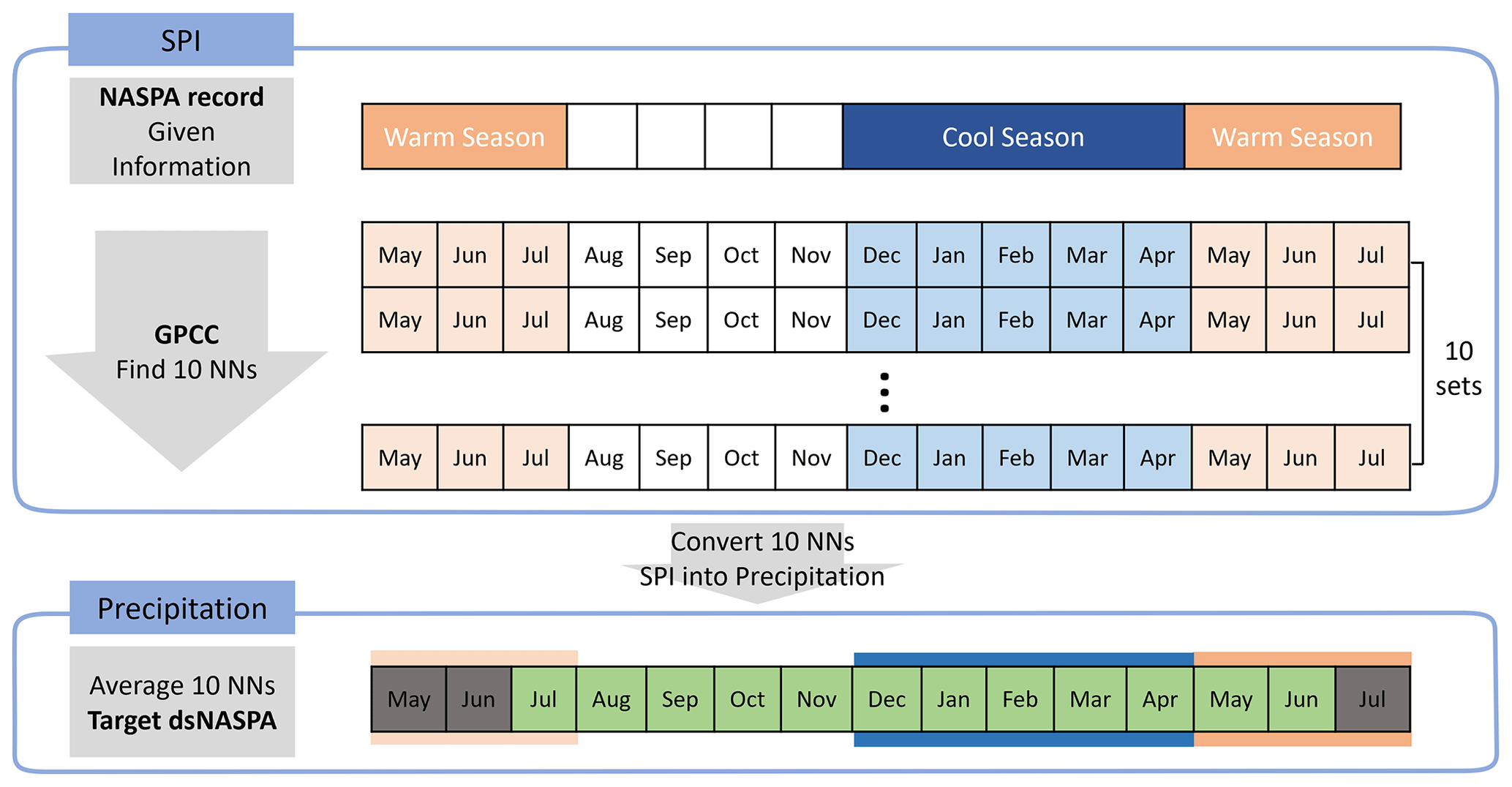
Figure 1 A framework for the temporal downscaling process. The monthly-scale (3-month average) NASPA precipitation time series is constructed using this process. This method is applied for every year of reconstruction. Note that “NNs” stands for nearest neighbors.

Figure 1 outlines the temporal-downscaling process using KNN. For each year, NASPA values were constructed as the target vector using three data points as follows: SPI-3 during the previous year's MJJ period, SPI-5 in this year's DJFMA period, and SPI-3 in this year's MJJ period. SPI-3 and SPI-5 values calculated from the GPCC instrumental period (1901–2013) for the same location were compiled to form the data library. The GPCC was used because it formed the basis for the original NASPA reconstruction (Stahle et al., 2020a). Second, for each year, we calculated the Euclidean distances between the target vector from NASPA and the available GPCC library to select 10 sequences (k= 10) from the GPCC SPI time series which have the closest Euclidean distance to the target NASPA SPI values. Note that resampled sequences are permitted to be any historical 13-month SPI series, regardless of whether the months align, increasing the number of available sequences from 113 (years in the GPCC dataset) to 1356 (years times months). This is possible because the SPI is agnostic to the season – each month follows a standard normal distribution. Then, the 10 resampled monthly SPI-3 time series were converted back to the 3-month precipitation using two-parameter gamma distributions derived from the GPCC dataset. Lastly, the 10 sets of precipitation time series were averaged and inserted into the targeted year of the NASPA.

Overall, our downscaling approach provides a few advantages. First, it reflects the compatibility of the climate field as it searches analogs from the same location. Second, direct resampling from the GPCC sample field based on similarity incorporates realistic seasonal progression and the 3-month structural persistence of the SPI. Third, the k neighbors create an ensemble of equally likely time series, identifying an envelope of feasible time series when there is no information between the three points from the NASPA reconstruction.

Downscaling skill was measured by means of the normalized mean absolute error (nMAE) using the following equation:

$$\begin{array}{}\text{(1)}& \mathrm{nMAE}={\displaystyle \frac{{\sum }_{\mathrm{Month},\mathrm{year}}\mathrm{|}\text{GPCC}-\text{NASPA}\mathrm{|}}{{\sum }_{\mathrm{Month},\mathrm{year}}\mathrm{GPCC}}},\end{array}$$

where GPCC represents the observed precipitation during the instrumental period and NASPA represents the ensemble mean of the reconstructed precipitation after applying KNN downscaling to the NASPA reconstruction.

2.4 Bias correction using the hierarchical GAM

Generalized additive models (GAMs) are statistical models that enable regression using nonlinear smooth functions instead of, or in addition to, linear covariates. GAMs are a subset of generalized linear models (GLMs), meaning their regression terms can represent parameters for data with distributions other than the normal distribution. However, while most GLMs apply linear regression principles to model a distribution's parameters, GAMs can include nonlinear terms (Simpson, 2018; Wood, 2008; Pedersen et al., 2019). When nonlinear terms are applied to time series data, GAMs also permit spanning irregularly sampled data to model complex and nonlinear drought trends. This method was applied to create a single common estimate of the temporally varying gamma distribution parameters representing precipitation climatology by incorporating information from multiple biased data products. We refer to the process of accounting for seasonal bias in the mean and shape parameters from different datasets as “bias correction” for the remainder of this paper, as it mirrors the process of bias correction by moment matching. However, unlike with a separate bias correction step, this is performed within the GAM, permitting confidence intervals around each of the bias correction terms.

GAMs have been previously applied to accumulated precipitation data to estimate the parameters of the two-parameter-gamma-distribution SPI under nonstationary climate conditions (Stagge and Sung, 2022; Shiau, 2020; Sung and Stagge, 2022). This study relies on the nonstationary SPI approach introduced in Stagge and Sung (2022) and applied in Sung and Stagge (2022). In this approach, the two parameters (mean and shape) of the gamma probability distribution are modeled as slowly changing through two covariates of time: year (to capture multi-decadal trends for certain months) and month (to capture recurring seasonality). Here, we expand this approach by adding a hierarchical grouping variable to simultaneously model common seasonal-specific long-term trends across datasets while incorporating variability at the group level, following the approach of Pedersen et al. (2019). When applied, this model decomposes information from all datasets (CRU, gridMET, and NASPA) into a smoothed long-term trend that is common to all datasets and into an additional annual seasonality smoother that varies slightly by dataset to account for bias relative to the gridMET dataset. In this way, there is a single common trend, with an adjustment added to shift the mean and shape parameters up or down seasonally based on the data source.

The detailed model framework is shown below in Eqs. (2)–(4). The gamma distribution is typically prescribed by shape and scale parameters (α and θ, respectively), but our approach follows Wood (2006), instead estimating the mean and shape parameters (Eqs. 3–4). The scale parameter can then be estimated from the mean and shape (Eq. 2).

$$\begin{array}{}\text{(2)}& {\displaystyle }\begin{array}{rl}& P_{\mathrm{3}\mathrm{month},m,y}=\mathrm{gamma}\left(\mathit{\alpha },\mathit{\theta }\right)\left(\begin{array}{c}m:\mathrm{month},\\ y:\mathrm{year}\end{array}\right),\\ & \mathrm{where}\mathit{\theta }={\displaystyle \frac{\mathit{\mu }}{\mathit{\alpha }}},\end{array}\text{(3)}& {\displaystyle }\begin{array}{rl}\mathit{\mu }& ={\mathit{\beta }}_{\mathrm{0}\mathit{\mu }}\left(\begin{array}{l}\mathrm{CRU}\\ \mathrm{NASPA}\\ \mathrm{gridMET}\end{array}\right)+{\mathit{\beta }}_{\mathrm{1}\mathit{\mu }}{f}_{\mathrm{s}\mathit{\_}\mathit{\mu }}\left(X_{\mathrm{month}},\mathrm{by}=\begin{array}{l}\mathrm{CRU}\\ \mathrm{NASPA}\\ \mathrm{gridMET}\end{array}\right)\\ & +{\mathit{\beta }}_{\mathrm{2}\mathit{\mu }}{f}_{\mathrm{te}\mathit{\_}\mathit{\mu }}\left(X_{\mathrm{year}},X_{\mathrm{month}}\right),\end{array}\text{(4)}& {\displaystyle }\begin{array}{rl}{\displaystyle \frac{\mathrm{1}}{\log \left(\mathit{\alpha }\right)}}& ={\mathit{\beta }}_{\mathrm{0}\mathit{\alpha }}\left(\begin{array}{l}\mathrm{CRU}\\ \mathrm{NASPA}\\ \mathrm{gridMET}\end{array}\right)+{\mathit{\beta }}_{\mathrm{1}\mathit{\alpha }}{f}_{\mathrm{s}\mathit{\_}\mathit{\alpha }}\left(X_{\mathrm{month}},\mathrm{by}=\begin{array}{l}\mathrm{CRU}\\ \mathrm{NASPA}\\ \mathrm{gridMET}\end{array}\right)\\ & +{\mathit{\beta }}_{\mathrm{2}\mathit{\alpha }}{f}_{\mathrm{te}\mathit{\_}\mathit{\alpha }}\left(X_{\mathrm{year}},X_{\mathrm{month}}\right),\end{array}\end{array}$$

where $P_{\mathrm{3}\mathrm{month},m,y}$ represents the 3-month moving average of precipitation at year y and month m. The precipitation is fitted to a gamma probability distribution, which has μ (mean) and α (shape parameter). The β are different parameters of the spline functions, f_s and f_te, which denote cyclic and tensor splines, respectively. The underlying principle of the model is that there is a single best estimate of the precipitation distribution at any given time. This is described by the mean and shape parameters of the gamma distribution that change seasonally, β₁f_s(X_month, by = dataset), and can also change slowly at a multi-decadal scale, f_te(X_yearX_month), with a constant y intercept, β₀(dataset). Similar to quantile-mapping bias correction (Lanzante et al., 2018; Ho et al., 2012), the ${\mathit{\beta }}_{\mathrm{0},\mathrm{model}}+{\mathit{\beta }}_{\mathrm{1}}f$(X_month, by = dataset) terms in both shape and mean parameters allow for adjustments based on the month and the model. The model is therefore capable of modeling trends and correcting data-induced bias simultaneously.

The single common tensor product spline smoother (f_te(X_year,X_month)) is shared across all datasets to model the interaction of long-term trends (X_year) relative to the season (X_month) using smoothly changing parameters for the two dimensions (year and month). A tensor product spline is an anisotropic multi-dimensional smoother, meaning it can model the interaction of variables with different units and can assign different degrees of smoothing for each direction, which is necessary for dimensions of month and year. Estimating β_2μ and β_2α in terms of years and months allows for nonlinear annual trends for each month while constraining these trends to be smooth through time. We constrain the smoother with control points (knots) every 70 years for mean and shape parameters to approximate climate variability at decadal scales while preventing excessive sensitivity/volatility. As such, the tensor product can simultaneously model seasonal precipitation regimes, shifts in those periods to earlier or later in the year, and nonstationary changes in the long term. The tensor spline approach of modeling trends in two time dimensions follows the methodology of Stagge and Sung (2022).

The first two terms derive the intercept and seasonality distinctive to each dataset. The first term, β₀(datasets), accounts for the dataset-specific intercept, and the second term, ${\mathit{\beta }}_{\mathrm{1}}{f}_{\mathrm{s}}\left(X_{\mathrm{month}},\mathrm{by}=\mathrm{dataset}\right)$, accounts for dataset-specific seasonality. Cyclic spline functions, f_s, were applied to model the seasonality term, assuming that a cyclic function for the recurrent monthly term constrains the model, so that late December and early January have similar values, matching with their second derivative. This term is stationary; i.e., it does not change from year to year. The term f(X_month by = dataset) uses group-level smoothers for this seasonal bias spline, meaning that each dataset applies unique seasonal adjustments to the common tensor product spline. A dataset-specific intercept, β₀(dataset), was also included to capture consistent biases between datasets. The variations in smoothing functions and parameter β are modeled using “mgcv” packages in R (Wood, 2008).

Bias correction was conducted based on three assumptions: (1) the gridMET dataset is not systematically biased (Yang et al., 2017); (2) the magnitude of bias can differ by season; and (3) biases are stationary in the long term – i.e., biases during overlapped periods are representative of biases throughout the rest of the data. Following the first assumption, when plotting results, we adjust CRU and NASPA parameters to match the gridMET dataset. The second and third assumptions are addressed by ${\mathit{\beta }}_{\mathrm{0},\mathrm{model}}+{\mathit{\beta }}_{\mathrm{1}}f(X_{\mathrm{month},}\mathrm{by}=\mathrm{dataset})$ permitting different bias corrections by month and model, which are estimated during overlapping periods and fixed outside these periods.

The significance of the modeled trend is tested using the instantaneous first derivative method. This method calculates the first derivative of the modeled trend with 1000 randomly drawn estimates of the modeled mean and shape parameters over time (by year). Then, we calculate the 95 % confidence interval around the first derivatives to indicate periods where the trend is significantly different from zero, i.e., where the trend is increasing or decreasing. The nonlinear trend analysis approach overcomes the limitation of simple linear significance tests, which only capture monotonic changes. Accordingly, it is not possible to discuss a single “trend”, but one can discuss whether the distribution mean is significantly increasing or decreasing at a given time, which is represented by the instantaneous first derivative. As such, this method has the benefit of preserving all nonlinear and nonstationary characteristics in modeled trends while providing estimates of significant changes. The results of this analysis are shown in Fig. S5 in the Supplement.

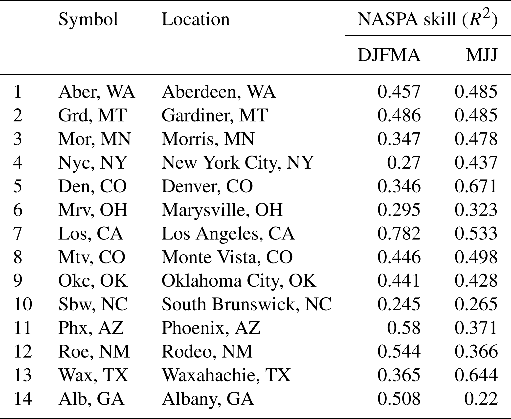
Figure 2 Gauge site locations. The abbreviations of the locations are as follows. 1: Aber, WA. 2: Grd, MT. 3: Mor, MN. 4: Nyc, NY. 5: Den, CO. 6: Mrv, OH. 7: Los, CA. 8: Mtv, CO. 9: Okc, OK. 10: Sbw, NC. 11: Phx, AZ. 12: Roe, NM. 13: Wax, TX. 14: Alb, GA.

The developed model was applied to 14 locations across the continental United States (Fig. 2; Table 1). These sites were chosen based on the availability of relatively long instrumental records, adequate NASPA reconstruction skill, and their representation of a wide range of climate regions. NASPA reconstruction skills are investigated using calibration and validation statistics by data creators (Stahle et al., 2020b). One of the calibration statistics, the coefficients of multiple determination (R²), is presented in Table 1. We avoid determining whether the datasets are acceptable or not through these statistics; rather, we aim to clarify which seasons or regions have better skills.

Table 1 List of sites considered in this study. The number assigned to each site refers to its location in Fig. 1. NASPA reconstruction skill for the cool (DJFMA) and warm (MJJ) seasons is presented in terms of R².

3 Results

3.1 Temporally downscaled monthly NASPA time series

In order to merge the NASPA data with CRU and gridMET data, the irregularly spaced NASPA must first undergo temporal downscaling, or disaggregation, to achieve a regular monthly time step and 3-month duration. The downscaled NASPA (dsNASPA) time series, averaged over 3 months, was constructed at a monthly scale and given the “ds-” prefix to distinguish it from the original NASPA reconstruction. Figure 3 shows 3 example years for two sites with very different climatologies, showing the ensemble of 10 selected nearest neighbors (pink); the resultant dsNASPA estimate (black); and the true value from the GPCC for the years when data are available, i.e. 1950 and 2010 (blue). Each figure displays 13 months, or one unit, of the KNN downscaling process – from the previous year's July to the current July. The downscaling results for all study sites are shown in Figs. S1 and S3.

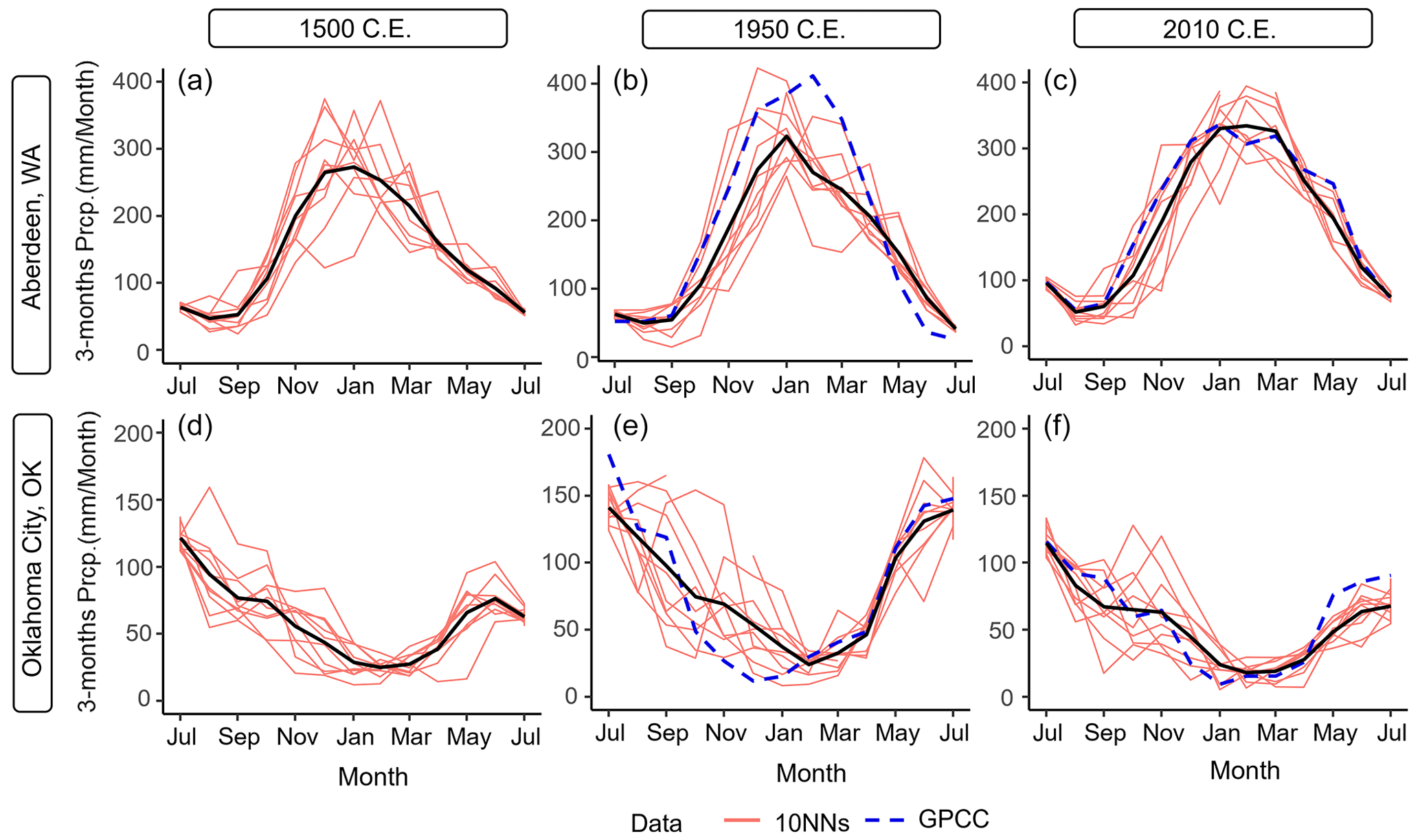
Figure 3 Comparing the downscaled NASPA (black line), 10 nearest neighbors (pink lines), and GPCC (dashed blue line) for Aberdeen, WA (a–c), and Oklahoma City, OK (d–f). The marked months on the x axis each refer to the last month of the 3-month rolling average. Prcp.: precipitation.

The dsNASPA generally agrees with the GPCC, especially with respect to capturing seasonality (Figs. 3 and S1). Downscaling skill is generally good in the season between December–February (DJF) and MJJ, where the NASPA reconstruction covers all 3 months (Figs. 3 and 4). The July SPI-3 (MJJ) often produces the smallest nMAE, which is logical given that the July SPI-3 period exactly overlaps with the warm season (MJJ) from the NASPA. Thus, the downscaling process has good information during this period and is not required to do as much.

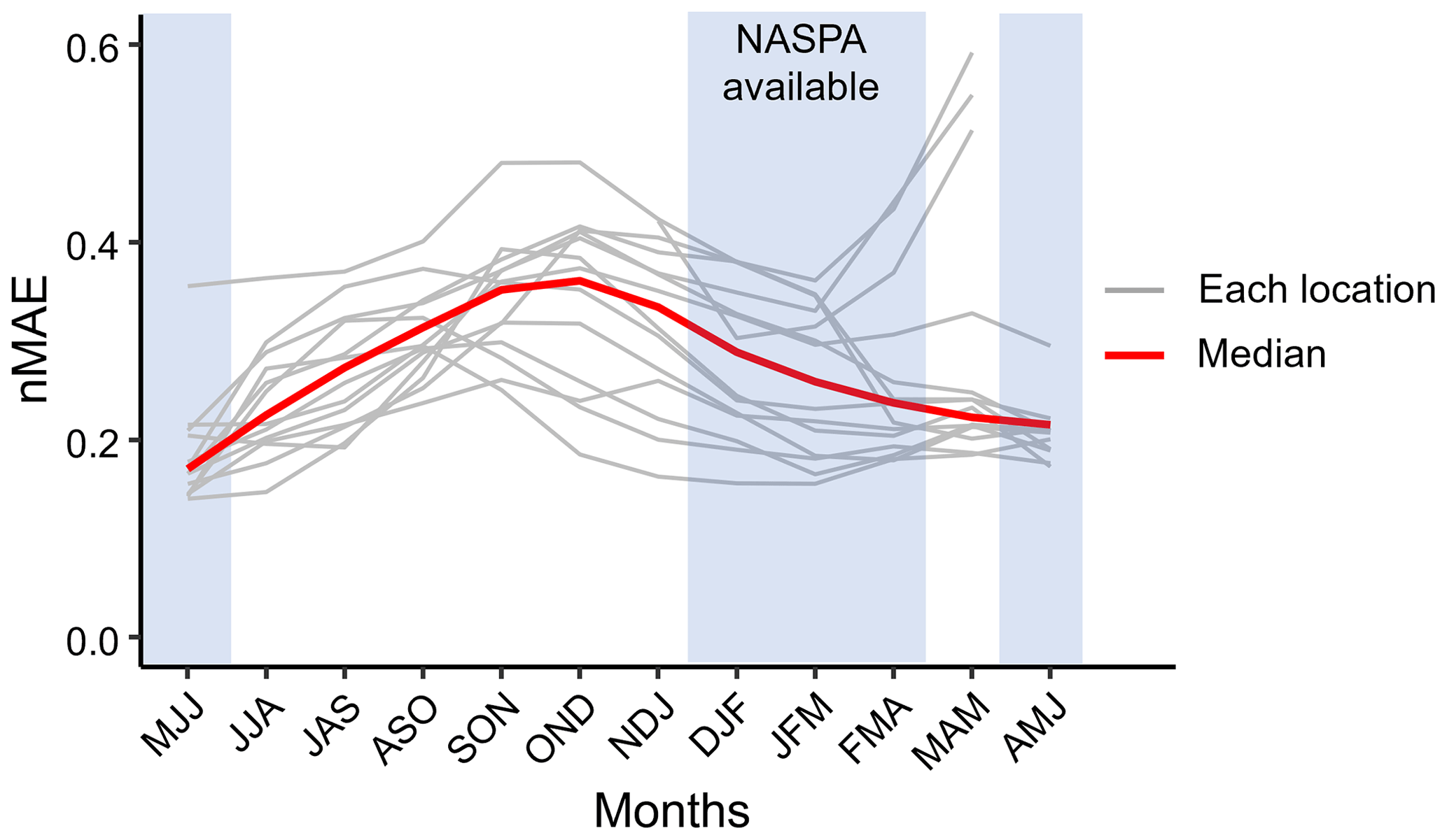
Figure 4 The nMAE indicating downscaling skill at each location (shown in grey) and the median nMAE (shown in red).

There are a few exceptions showing the best skill during winter (DJF) and poor skill, with a large nMAE, during early summer (MJJ, Fig. 4). This occurs only in the southwestern US (i.e., Los Angeles, CA; Phoenix, AZ; and Rodeo, NM), where the underlying NASPA shows better initial reconstruction skill during the region's relatively mild winters (Table 1) and less skill in summer. For the dsNASPA, the seemingly large errors in the nMAE during MJJ are primarily due to extremely small values in the denominator of the nMAE as a result of very low precipitation, combined with the fact that infrequent large rainfall events are not captured. Figure S3 illustrates that a few large precipitation events in these regions drive a large nMAE (scatterplot); however, the dsNASPA still matches the GPCC (time series) well. Despite this limitation, downscaling accurately predicts the general precipitation pattern in terms of seasonal and long-term average precipitation, with nMAE values generally between 0.1–0.5. We compared the performance of the dsNASPA with a highly naive alternative (assuming the mean of the GPCC climatology) and found that the dsNASPA provides a clear signal in the period with NASPA information (blue-shaded area in Fig. 4). As expected, the dsNASPA provides less information in the interpolation period where NASPA estimates are not available. However, during the gap seasons, the dsNASPA still produces a positive correlation with observations, useful for measuring climatological shifts, and greatly reduces extreme errors created by the naive estimator in the semiarid west. For regions other than the semiarid locations described above, errors during periods of good NASPA coverage occur primarily due to the errors between the sampled GPCC and NASPA (Fig. S3). For example, the dry bias shown in July (MJJ) between the dsNASPA and GPCC in 1950 for Oklahoma City, OK (Fig. 3e), is caused by uncertainty in the original NASPA dataset, which caused the converged point of the nearest neighbors (black) to underestimate precipitation relative to the GPCC observation (blue). May and June (MAM, March–May, and AMJ, April–June, respectively) are reproduced nearly as well, given that these periods share coverage from the cool (DJFMA) and warm (MJJ) reconstructions.

Later periods of the 5-month cool-season reconstruction, January–March (JFM) and February–April (FMA), show reasonably good accuracy. Error increases during fall and winter across a temporal gap between NASPA reconstructions (Figs. 4 and S3). This is indicated by much broader resampled estimate ranges (Figs. 3 and S3) during the late fall and early winter.

3.2 Investigating model bias

Here, we investigate how dataset bias is quantified in the model. As mentioned, our model accounts for two types of bias: a consistent bias for a given dataset across the entire year and seasonal-specific bias. These bias terms were estimated for both the mean and shape parameters.

Typical results for the Monte Vista, CO, gauge show how these biases are captured in a single model. Figure 5 shows the nonstationary mean estimate for each dataset, represented by the colored lines, and the SPI ranges of −1.5 to +1.5 (grey-shaded regions). Note that the nonstationary mean lines all follow the same trend and are simply adjusted up or down based on bias. At this station, dsNASPA and CRU datasets tend to underestimate precipitation relative to the gridMET benchmark across all four seasons. This consistent offset may be due to the significantly coarser resolution of the NASPA and CRU datasets, which may not capture elevation effects, particularly in this mountainous region. The magnitude of bias also differed by season in this example, with the greatest differences visible during the August–October (ASO) season (Fig. 5). Note that the four periods we highlight in this study were purposefully chosen to mimic NASPA availability, anchored by the 3-month MJJ period, rather than the more commonly used seasons (DJF, MAM, JJA, SON).

Figure 5 Long-term trends for each dataset for four periods at the Monte Vista, CO, site. The modeled long-term trends for the datasets are represented as differently colored lines, while the SPI ranges (−1.5 to 1.5) for the datasets are indicated by grey regions.

In addition to detecting bias in the mean parameter, it is possible to detect model bias in the shape parameter, which controls variance, and thus identify the range between SPI −1.5 and +1.5. The most notable bias in the shape parameter for the Monte Vista, CO, example is for the dsNASPA, particularly during ASO, where the shape parameter is significantly overestimated, thereby decreasing the variance for the same mean (Fig. 5). This is logical, as the ensemble resampling approach likely decreased extremes for the ASO period, for which there is no direct NASPA information. The shape parameter bias is negligible for the FMA and MJJ periods, which have full NASPA coverage. Shape parameter bias results for Monte Vista, CO, are typical of those for other gauges studied here, with the largest bias exhibited during the interpolated ASO period and little bias observed in periods with good NASPA information.

We present results for all other regions in Fig. S4. The results indicate that the shape biases are largely dependent on the season, whereas the mean biases are more dependent on the gauge. Notably, the ASO season shows large biases in the shape parameter. This is primarily because the dsNASPA for this season cannot represent occasional extreme precipitation values, leading to an underestimation of its variance. In contrast, the MJJ season shows considerably less bias since the dsNASPA was developed from complete precipitation estimate from the NASPA. A few exceptions exist in Monte Vista, CO, and Gardiner, MT, where there are large biases in the mean parameters across all seasons, possibly due to topographic effects between the gauge locations in these mountainous regions.

3.3 Constructing long-term trends

By accounting for the model-induced bias described in Sect. 3.2 and adjusting all datasets to match the gridMET dataset, we were able to generate a 2000-year model of nonstationary precipitation trends for each gauge. The modeled long-term trends incorporating bias correction across all instrumental and proxy datasets for Albany, GA, and Monte Vista, CO, are presented in Fig. 6 as examples to illustrate the results of this approach. Figure 6 represents the long-term mean for each season as a line with a shaded range between SPI = −1.5 and +1.5, similar to Fig. 5. The solid black line shows the common long-term trend of the mean, while the precipitation series are shown as raw data without bias correction for context. Figure 6 focuses on the period 1400–2020, when the original NASPA dataset has the best reconstruction skills (Stahle et al., 2020a).

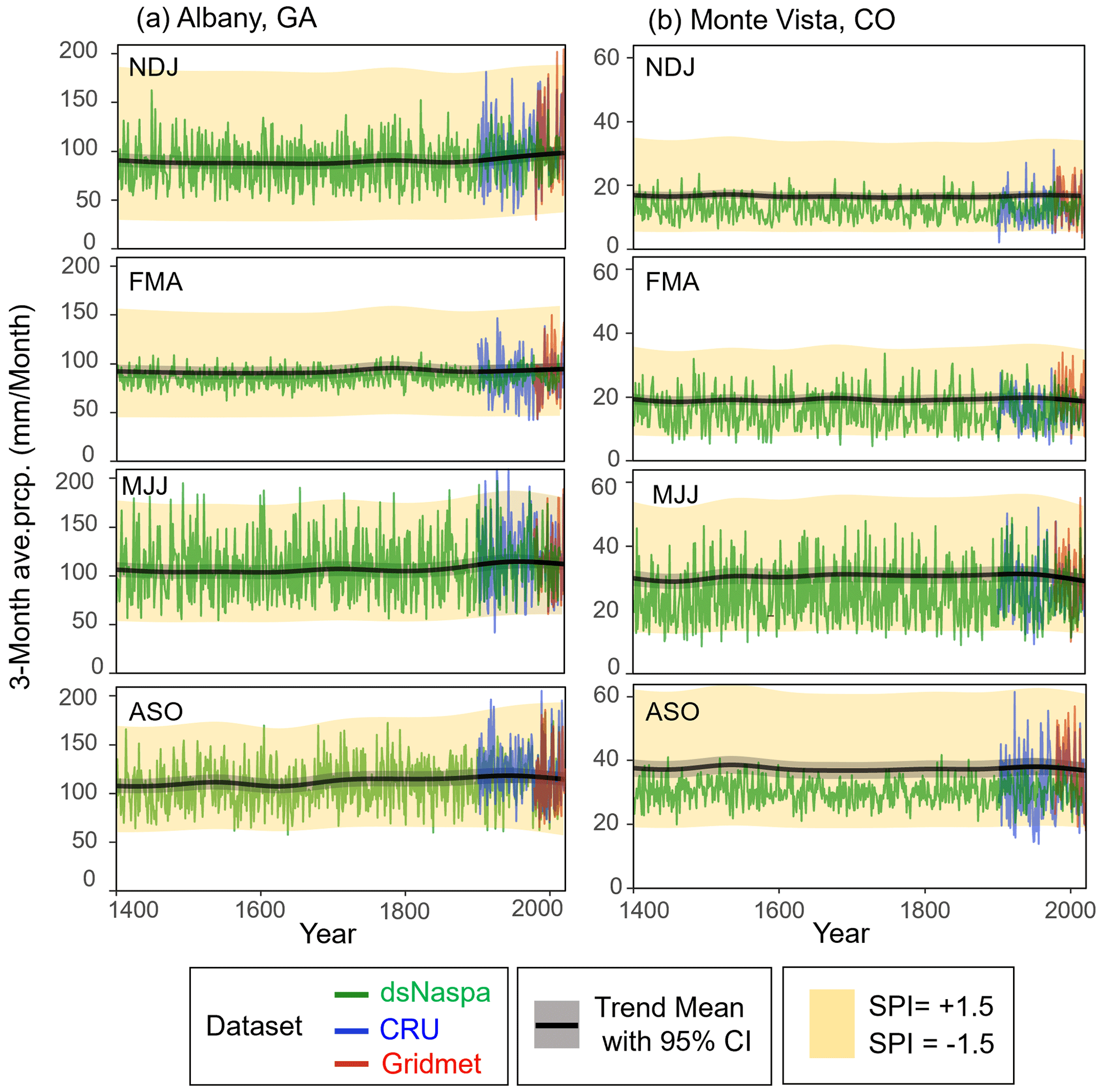
Figure 6 Long-term trends in the 3-month nonstationary standardized precipitation index (NSPI) (black line) and illustrations of averaged precipitation for four periods at the Albany, GA, and Monte Vista, CO, sites. The yellow-shaded area represents the precipitation amount between SPI $=+$1.5 (upper boundary) and −1.5 (lower boundary) in the fitted gamma distribution. Trends in the mean and SPI range (−1.5 to +1.5) are shown using gridMET data as a baseline to illustrate bias correction, while the raw data are shown without bias correction for context.

It is noteworthy that all seasons in Albany, GA, have experienced noticeable trend changes in recent years, but the direction of change differs by season. Figure 6a shows the warm season (MJJ) has underwent a long-lasting wetting trend from the 1800s to 1900s, followed by a drying trend during the 20th century in both the mean (SPI = 0) and wet anomalies (SPI = 1.5). November–January (NDJ) shows a wetting trend beginning in the mid-1800s and continuing to the present for both wet and dry anomalies. The NDJ mean in current years (2000–2020) shows the wettest condition of the last 1000 years (Fig. 6a). This agrees with previous findings using the NASPA dataset, which have identified the Southeast US (including Albany, GA) as experiencing the greatest positive precipitation trend during the cool season (Stahle et al., 2020a).

We note that the Albany, GA, site has also experienced changes in the magnitude of variability between dry and wet extremes. The range between SPI = 1.5 and SPI = −1.5 became much larger during the recent period, particularly for the ASO season, implying that both wet and dry anomalies have become more extreme than during prior centuries. The strong drying trend during MJJ coupled with a wetting trend during the NDJ season indicates a seasonal shift in the driest season. While NDJ has historically been the driest period among the four seasons, during the modern period, MJJ now has similar dry conditions to those observed during the NDJ period.

Monte Vista, CO, had very stable SPI trends until the 19th century before undergoing a rapid drying trend during the 20th century, particularly during the MJJ and ASO periods (Fig. 6b). The modeled MJJ precipitation with normal climatology (SPI = 0) is currently at its driest in approximately 500 years, following a long stable period between 1500 and 1900. ASO also shows drying trends over the last 300 years.

We can see that the modeled mean of the dsNASPA in Monte Vista, CO, is shifted upwards from its original average value because of bias correction adjustment to match the slightly drier dsNASPA climatology with the slightly wetter gridMET climatology for this site (Fig. 5). Our modeling process detected these biases and calibrated them to shift upwards while maintaining a common gradual trend.

Figure 7 Long-term trends in 3-month average precipitation (mm month⁻¹) for four seasons. In each panel, the period before 1400 is shaded to represent the period with less prediction skill in the original NASPA.

Figure 7 shows long-term trends for the four previously discussed seasons across all 14 study sites. The statistical significance of these changes is observed in Fig. S4. The plots show natural seasonality as the difference between the seasonal lines and the long-term climate nonstationarity changes in each line. This separation allows for an evaluation of recent precipitation trends by comparing the past 100-year trend with the longer 2000-year time window. While results from the entire nonstationary GAM (extending back to the earliest NASPA reconstructions) are presented in Fig. 7, our primary focus is on the period after 1400, shown in white. Prior to 1400, the NASPA reconstruction has greater uncertainty and is thus provided here for full context but shaded in grey to emphasize this greater uncertainty. Figure 7 shows that the 14 demonstration sites generally follow a spatial climate pattern found in previous studies, which illustrates industrial-era drying trends in the southwestern US and wetting trends in the eastern US (Lehner et al., 2018; Prein et al., 2016; Ellis and Marston, 2020). The drying trend in the west is most prevalent during each site's wet seasons, with smaller or negligible trends during the driest part of the year. For example, the wet-season drying trend is visible in Aberdeen, WA, where after several centuries of stable precipitation there has been a decrease during the cool wet seasons (NDJ and FMA). The wet season (FMA) in Gardiner, MT, and Los Angeles, CA, also shows clear drier trends during the most recent century or longer. The drier trend in Los Angeles, CA, during FMA precipitation has declined since 1500, but this trend was exacerbated and became more severe during the 20th century, effectively shortening the wet winter period prior to the region's dry summer. The 20th-century drying trend in Monte Vista, CO, has occurred across all seasons, not only during the wettest period as in the other western stations. The most severe drying trend occurred in MJJ, as mentioned in the previous section (Fig. 6). The most severe western sites illustrate the value of comparing 20th-century drying trends to longer reconstructed records to identify rapid and exceptional precipitation changes. Unlike these western sites, Denver, CO, shows negligible long-term trends, while the desert southwest (Phoenix, AZ, and Rodeo, NM) exhibits minor wetting trends which are largely within the pre-industrial historical range.

The eastern part of the US generally has experienced rapid wetting trends during the most recent century, as observed in previous research (Bishop et al., 2021). These wetting trends are especially drastic in New York City, NY; Morris, MN; and Marysville, OH, each currently experiencing the wettest conditions of the last 500 years of pre-industrial, presumed near-natural, cyclic variability. This pattern is particularly visible for the warm and wet summer season (MJJ). South Brunswick, NC, also shows a wetting trend during all seasons since 1700, but these trends are not as rapid as those observed in the more northern sites. Warm-season (MJJ) precipitation has also increased in the Southern Plains (Oklahoma City, OK, and Waxahachie, TX). Precipitation during the summer season has been gradually increasing since 1400 but has undergone far more rapid increases since 1900. Note that nonstationarity in the eastern US is less stable; this may be related to greater uncertainty in the NASPA reconstructions for this region, which generally exhibit poorer reconstruction skill (Table 1, Stahle et al., 2020a).

Some locations have experienced different directions of changes based on seasons. These changes mostly occur in the southern part of the US, as shown in Fig. 7 (11)–(14). For example, FMA precipitation in Phoenix, AZ, has become slightly wetter during the last 500 years, while the other three seasons were slightly drier during the 20th century. Albany, GA, shows recent drying trends during the spring and early summer (FMA and MJJ) but wetter trends during fall and winter (ASO and NDJ). These seasonal-specific changes ultimately shift the timing of the wettest or driest season. For example, while the NDJ season has been the driest season during the past 500 years, slightly drier than the preceding ASO season, this changed during the 20th century. In addition, the difference between the wet seasons (February–June) and dry seasons (August–January) is decreasing as the wet seasons become drier and the dry seasons become wetter. Seasonal shifts also appeared in Waxahachie, TX, stemming from a constant wetting trend during the MJJ season since the year 1000, while other seasons have experienced what is presumed to be natural variability with no abrupt 20th-century changes, although further analysis is required to quantify the impact of natural variability. Though not the focus of this study, our results do capture past drought events, such as the prolonged dry period in the 1200–1300s in Oklahoma City, OK, and Waxahachie, TX, which is consistent with previous studies regarding the so-called medieval megadrought (Stahle, 2020; Cook et al., 2016).

4 Discussion

Our novel approach for temporal downscaling, combined bias correction, and nonlinear-trend modeling enables analyses of meteorological drought changes at a multi-centennial scale. Our downscaling approach allows irregular historical reconstruction to be included with instrumental records in a single long-term-trend model using the same temporal scale, and ultimately, it allows us to compare nonstationary drought trends across seasons. The KNN-downscaling approach preserves greater certainty during seasons with NASPA reconstructions and greater uncertainty during seasons that must be interpolated. Simultaneous temporal trend fitting and bias correction, constrained with a GAM spline, appear to provide a stable framework for merging these disparate datasets.

When developing the KNN approach, we chose to consider 13-month time segments regardless of seasonality, which may not capture some higher-order characteristics, such as seasonal correlation. This design decision was a trade-off between the benefits of a larger sampling library of feasible SPI traces and the risk of overlooking some seasonally specific time series behavior. We chose the former, with an additional assumption that anchoring the time series behavior at three seasonal points would likely lead to oversampling of segments with similar seasonal behavior. Also, our process of selecting SPI sequences and converting back to precipitation based on the seasonal probability distribution reflects the region's seasonal characteristics. This is demonstrated in Fig. S1, showing that our dsNASPA captures the general seasonality well. Nevertheless, future research might explore the magnitude of seasonality effects and the persistence of SPI sequences in the downscaling process.

We also acknowledge the uncertainties concerning the whole modeling process. The uncertainties in the dsNASPA stemming from the downscaling process in addition to the original reconstruction process vary by region and season. As shown in our results, the downscaling skills are much higher in the period where the original NASPA provides information (Figs. S1 and S4). Reconstruction skills in the original NASPA vary depending on the region. This has been investigated in previous studies and data sources (Stahle et al., 2020a). In addition, stationarity in bias is an assumption of this method; however, it is a necessity that underlies most proxy reconstructions. Based on prior NASPA validation, we are most confident that bias remains consistent during the period with consistent tree-ring coverage (1400–present; white area in Fig. 7) but may begin to change as chronology-based coverage and reconstruction skill decrease (before 1400; grey-shaded area in Fig. 7).

Nonetheless, our primary objective is to realize the best possible estimate of the changes in precipitation distributions (climatology) of the past rather than to replicate specific events in the time series. If one is interested in predicting precipitation in a given year, we recommend using the original NASPA dataset rather than our dsNASPA interpolation. Overall, our derived gamma distribution can be used to understand the most likely climatology of the past, and potentially the future, based on available data.

In this context, our KNN approach creates a plausible estimate for periods lacking NASPA estimates (e.g., ASO) and is apt for estimating smooth changes in the distribution of historical climatology. Additionally, we found that taking the mean of neighbor ensembles did not artificially and dramatically decrease the variance (Fig. S1), further supporting our approach.

In particular, this approach appears successful at generating a continuous sequence of bias-corrected precipitation distributions while addressing some of the nuances of the NASPA reconstruction. The NASPA contains internal bias with respect to reconstructing precipitation for the cool and warm seasons, with skill varying across the continent. Further, within the cool or warm period, the reconstruction can be dominated by 1 or 2 months. For example, the DJFMA reconstruction in Los Angeles, CA, displays significantly higher correlations with precipitation totals for December, January, or February than with those for March or April. However, DJFMA was used as a compromise to ensure a common cool period across the US. It appears that hierarchical GAM bias correction combined with KNN downscaling mitigates some of this effect by creating a local model for each site. Further, by using a seasonally varying bias correction, the model adjusts to the months, such as those in DJFMA, that are best captured.

We found a general drying trend for the wettest seasons in the western US and wetting trends for most seasons in the eastern US. For some of these sites, 20th-century trends appear to be rapid and outside the range of the long-term reconstructed record, whereas for other sites, these patterns could be considered within the pre-industrial range and perhaps part of natural climate variability. Our results also pointed out some study sites where precipitation trends differ by season, leading to slightly altered seasonality.

Results for the case study at Los Angeles, CA, agree with general findings that showed extraordinary drying trends in the western US during the last century, following a prolonged period of stable precipitation patterns since the 1500s (Stahle, 2020). The previously documented medieval megadroughts in the Great Plains region (Cook et al., 2016) also appear in our results. This consistency of results indicates that incorporating NASPA reconstructions data using our new method is feasible and can be useful for identifying low-frequency drought trends and variability over the past 2000 years.

By contrasting the severity of precipitation changes during the past century with 2000 years of data, this model provides the potential to analyze the magnitude of recent trends during the modern increase in greenhouse gases along with pre-industrial natural variability. For example, Figs. 5, 6b, and 7 each present panels showing the same results from the meteorological drought trend model for Monte Vista, CO. Each successive figure takes a wider temporal viewpoint – from the last 120 years (Fig. 5) to the last 600 years, including the pre-industrial period (Fig. 6b), and the widest possible viewpoint, beginning in 0 CE (Fig. 7). As can be seen, the drying trends in Fig. 5 rather steadily decrease but do not capture the extraordinary changes shown in Fig. 6b. Taking a longer perspective implies that the modern 120-year data period is outside of the “pre-industrial levels” defined by UN Paris Agreement (IPCC, 2014), with the modern MJJ mean at its driest in 600 years. Our results agree with other findings that have identified recent or projected future shifts in seasonal precipitation (Marvel et al., 2021) or enhanced precipitation variability (Williams et al., 2020) due to anthropogenic climate change. For example, for several western sites, this study observed rapid drying trends during the wettest seasons (Aberdeen, WA; Monte Vista, MO; Gardiner, MT; Los Angeles, CA). These wet seasons are particularly critical in the western US, where seasonal precipitation is relied upon to fill reservoirs for later use during dry seasons. We therefore believe that modeling these smooth seasonal shifts over multiple centuries can inform water management plans to adapt to a changing climate. In addition, we believe that understanding the seasonal-specific changes in meteorological drought can help to analyze seasonal shifts in other types of droughts, such as anticipated soil moisture drought in the summer in the southwestern US due to declining spring precipitation (Williams et al., 2020).

We expect that our approach, described here as a model validation for several case study sites, could be applied across a denser network of sites to determine how meteorological drought has changed during the modern instrumental period and to put these trends into a much wider, pre-industrial context. A unique benefit of this approach is that it models nonlinear changes in typical precipitation (SPI = 0), dry anomalies (SPI < 0), and wet anomalies (SPI > 0) simultaneously across all seasons.

5 Conclusion

This study introduced a novel method designed to apply the recently introduced nonstationary SPI approach (Stagge and Sung, 2022) to a multi-centennial temporal scale by merging disparate datasets with a common tensor product spline term. To accomplish this objective, first, we downscaled the irregularly spaced, biannual NASPA reconstruction into 3-month average precipitation with a monthly resolution using a KNN approach. This permits analyses at a seasonal scale and enables the NASPA reconstruction to be integrated with instrumental data. In accordance with findable, accessible, interoperable, and reusable (FAIR) data principles, we make our data publicly available to allow researchers to access them and develop future drought trend studies (Wilkinson et al., 2016).

Second, we identified unique biases arising from different precipitation data sources and accounted for these biases in a hierarchical GAM with model-based bias correction. This model corrected both persistent biases and seasonal-specific biases in both mean and shape parameters of fitted distributions. Accounting for unique seasonal biases is important as previous studies have found that bias magnitude can vary by season (Piani et al., 2010; Li et al., 2010). This is especially relevant when merging the NASPA with observation datasets because the temporal downscaling procedure depends strongly on the season; e.g., MJJ is made directly from the original reconstruction, while ASO is based on KNN interpolation between the prior MJJ and the future DJFMA.

Third, after confirming that the temporal downscaling and nonstationary SPI model with bias correction were able to capture long-term trends, this study applied the model to a wide range of case study sites. Analyzing long-term trends in each season allows for the observation of shifts in seasonality and its variability. These changes are also captured by season, meaning that our study could point out a specific season that is experiencing rapid changes, although other seasons are not experiencing drastic changes.