A generalised ecohydrological landscape classification for assessing ecosystem risk in Australia due to an altering water regime

Describing and classifying a landscape for environmental impact and risk assessment purposes is a non-trivial challenge because this requires region-specific landscape classifications that cater for region-specific impacts. Assessing impacts on ecosystems from the extraction of water resources across large regions requires a causal link between landscape features and their water requirements. We present the rationale and implementation of an ecohydrological classification for regions where coal mine and coal seam gas developments may impact on water. Our classification provides the essential framework for modelling the potential impact of hydrological changes from future coal resource developments at the landscape level.

We develop an attribute-based system that provides representations of the ecohydrological entities and their connection to landscape features and make use of existing broad-level classification schemes into an attribute-based system. We incorporate a rule set with prioritisation, which underpins risk modelling and makes the scheme resource efficient, where spatial landscape or ecosystem classification schemes, developed for other purposes, already exist.

A consistent rule set and conceptualised landscape processes and functions allow for the combination of diverse data with existing classification schemes. This makes the classification transparent, repeatable and adjustable, should new data become available. We apply the approach in three geographically different regions, with widely disparate information sources, for the classification, and provide a detailed example of its application. We propose that it is widely applicable around the world for linking ecohydrology to environmental impacts.

1 Introduction

The categorisation of the Earth's surface into geo-ecological landscape classes provides a way to simplify the complexity of the form and function of the landscape and provides vital contextual information to support land and water management as well as policy initiatives. This includes identifying geographical regions within which landscape-scale attributes, such as climate, topography, geology and land cover, are homogeneous and distinctive compared with other regions. It involves identifying broad-scale, general patterns, processes and functions. Landscape class units are “ecologically equivalent”, having the same dominant processes that sustain a similar suite of species, and are likely to respond in similar ways to management initiatives or environmental changes. This ecological equivalence enables the selection of assessment locations for monitoring, measurement or experimentation, and it enables the extrapolation of results to all areas within the same ecological class (Hawkins and Norris, 2000; MacMillan et al., 2003; Cullum et al., 2016a, b).

Such a landscape classification also explains variation in ecological characteristics (e.g. assemblage structure) and is predictive of the ecological attributes of those areas. This predictive quality is useful for defining ecological criteria; identifying reference and degraded sites; defining conservation goals, including the assessment of biodiversity; and the setting of restoration objectives (Hawkins et al., 2000; McMahon et al., 2001; Snelder et al., 2004).

In summary, landscape classification is a way of dividing a landscape into components where the characteristics within the components are more similar than the characteristics between the components. That is, the components have their own distinct features that separate them from the other components.

However, describing and classifying a landscape for environmental impact and risk assessment purposes is a non-trivial challenge in areas where hydrological records are limited (e.g. Wolfe et al., 2019). This is the case for many regions in Australia, where low population densities, high urbanisation and limits on (water) resource management information exist. For our purpose, which was the assessment of risk to ecosystems within the regions of the Bioregional Assessments Programme (Bioregional Assessments, 2018), we needed a landscape classification that reflected the hydrological connectivity of surface and groundwater with ecosystems in the landscape. The Bioregional Assessment Programme, an Australian regional-scale impact assessment, investigated the impacts and risks of coal seam gas (CSG) and large coal mining developments on water resources and water-dependent assets via a water pathway (Bioregional Assessments, 2018). This investigation focussed on the landscape level – that is, on areas within the regions where the landscape is made up of different interacting land uses and ecosystems.

In our case, the broad-scale assessments of impacts from resource developments on ecosystems required an understanding of landscape composition and structure and of how these relate to the ecosystems embedded in the landscape. The type and composition of the landscape components are dependent on the focus of the assessment and, therefore, require careful consideration of the questions that the assessment seeks to answer (Wiens and Milne, 1989; Eigenbrot, 2016). For Australia, there are several landscape-level classifications available (e.g. Thackway and Cresswell, 1995; Pain et al., 2011; Hall et al., 2015; NVIS Technological Working Group, 2017; Gharari et al., 2011). Unfortunately, these available classifications are not directly applicable for our assessment regions because there is no alignment between the regions and existing classification boundaries, or the classifications, even if they include ecohydrological elements, are limited to their locations or domain of interest.

Identifying the water dependency of landscape components is a prerequisite when analysing the potential impacts of proposed coal and gas resource developments on water resources at a regional scale. For example, coal resource developments generally need to manage both groundwater and surface water as part of their operations. With multiple developments within the one region, impacts are likely to go beyond the local scale and affect ecosystems at the landscape level (e.g. Bioregional Assessments, 2018, 2019). In this context, there is a need for an ecological classification of the landscape that identifies and causally connects the water dependency of its components to activities of resource extraction, in a spatially explicit manner. Further, there is a need to identify impact pathways between resource extraction sites and the ecosystems that show causal connectivity between extraction activities and ecosystem impacts.

Land classification systems reveal patterns and underlying drivers of ecosystem structure and function, or they produce a tractable unit of assessment for evaluating environmental change (Hobbs and McIntyre, 2005; Poff et al., 2010). Many different classification approaches and methodologies currently exist to represent ecosystems in a landscape. This includes the Interim Biogeographic Regionalisation for Australia (IBRA), which provides the basis for defining and managing the national reserve system, and the National Vegetation Information System (NVIS), which describes the extent and distribution of vegetation ecosystems for the Australian continent (Thackway and Cresswell, 1995; Department of Agriculture, Water and the Environment, 2021). Classifications addressing hydrology in Australia incorporate a framework for river management that delineates boundaries between homogenous landscape components, based on either their dependency on surface water or groundwater regimes (Poff et al., 2010; Aquatic Ecosystems Task Group, 2012; Olden et al., 2012). However, none of these classifications describe ecohydrological connections between waters and the wider landscape. For example, IBRA and NVIS are based purely on vegetation classifications and, thus, do not contain any hydrological details, while the available hydrological classifications focus purely on the streams and waterbodies within the landscape, as their centre of attention is aquatic organisms and environmental flows. While both of these elements are part of the immediate landscape surrounding waterbodies, they do not in themselves provide conceptual and direct linkages between changes in water and ecosystem responses in the wider landscape. Therefore, a standardised approach to formulating classifications that combine these two aspects, ecosystems and their water sources, is lacking.

This conundrum exists because different analysis contexts require classifications for different purposes, such as conservation planning, habitat mapping, resource assessment and vegetation modelling, and because there is contention between the generality of broad classifications and their applicability at the local scale (Leathwick et al., 2003; Abella et al., 2003; Poulter et al., 2011; Cullum et al., 2016b; Pyne et al., 2017). Hence, we needed a new classification system for evaluating water dependency in the regional-scale context for multiple coal and coal seam gas resource developments. This new system must incorporate surface water and groundwater regimes into a spatial demarcation of ecosystem boundaries in the landscape. Including surface water and groundwater regimes will provide conceptual connection between impacts from developments on surface water and groundwater within the classification. The classification must also be spatially explicit to enable a landscape-wide analysis of those impacts, so that changes in water in one part of the landscape can be linked to ecological responses in another part of the landscape.

With this context in mind, the objectives for this paper are as follows:

1. characterise a regional-level landscape based on patterns in land use, ecology, geomorphology and hydrology;

2. develop landscape classes of water-dependent, remnant and human-modified features; and

3. ensure landscape classes sit within a common framework that aids in formulating conceptual models and patterns of water dependency across the landscape.

Here, we present the rationale, formulation and implementation of an ecohydrological landscape classification. Based on a generalised conceptual model of the typical hydrological connectivity within landscape features in a region, the classification integrates pre-existing, broad-level classification schemes into an attribute-based schema applied at the regional scale. It places the landscape classification within a common framework (i.e. a framework that is common to all landscape elements in the region) that aids in formulating conceptual models and patterns in water dependency across the landscape. This makes our approach generally applicable for assessments aimed at regional hydrological impacts on, and risks to, ecosystems. Importantly, the classification also provides the ability to develop a conceptual understanding of, and causally connect, hydrological changes at the landscape level with impacts on ecological entities within the landscape. These causal pathways are the basis for spatially identifying the impacted areas and for developing an appropriate mitigation response, including for extractive resource developments and water extraction.

We have applied this approach to several regions across eastern Australia with coal and CSG resource developments. Here, we will focus on its application in three regions – Namoi, Maranoa–Balonne–Condamine and Galilee – and subsequently discuss why the approach is transferable to other regional developments that may carry a hydrological-based risk to ecosystems, even those in a different contextual setting with regards to data sources and existing landscape classifications.

The remainder of the paper is structured as follows: Sect. 2 describes the general approach for achieving the classification, including descriptive examples of existing data sources. It also provides a description of the three study regions in which we applied and tested the classification. Section 3 provides evidence of the general applicability of our approach in that it shows the detailed ecological landscape classification for the three distinctively different regions in terms of location, topography and climate. In Sect. 4, we provide an example of the use of the landscape classification. Here, we describe an impact assessment in the Namoi region using modelling that includes expert assessments. In the last section (Sect. 5), we provide a discussion of the landscape classification, including limitations, and provide our conclusions.

Figure 1 provides a visual outline of the paper and workflow applied. It incorporates Sects. 2, 3 and 5 (unshaded parts) and indicates where we applied our classification using quantitative and qualitative risk modelling in combination with surface water and groundwater modelling (shaded parts; Sect. 4). Surface water and groundwater modelling establishes a zone of hydrological change in which impacts are likely. The red, more lightly shaded circle shows the resulting risk assessment outcomes, where the landscape classification provided the crucial details for experts to assign risks to landscape elements and classes.

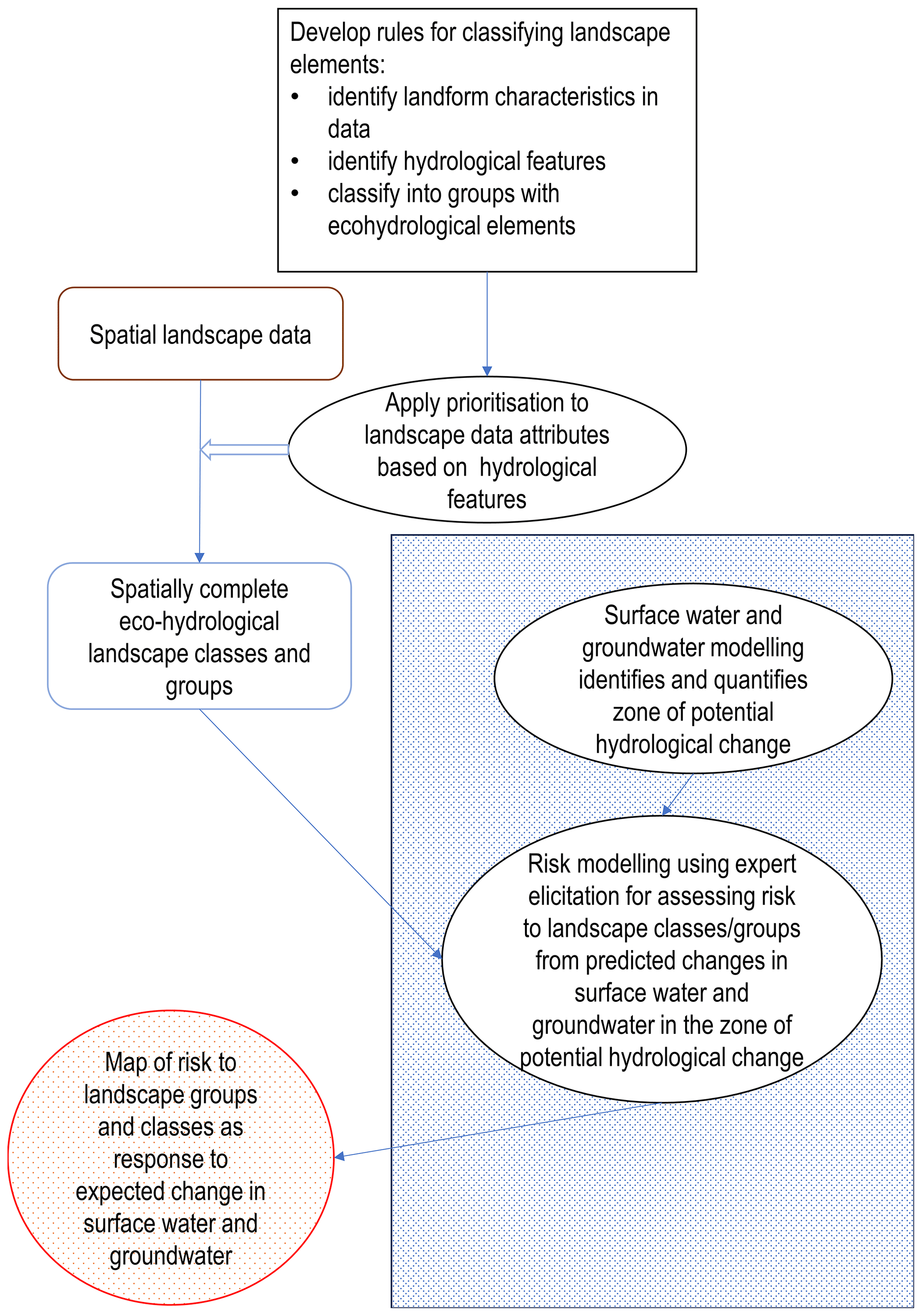
Figure 1 Visualisation of the workflow for developing our ecological landscape classification (non-patterned area – identifies the focus of this paper) and its application in an ecological risk assessment, which we briefly summarise to show the classification's applicability (inside patterned rectangle – described in Sect. 4). The outcome of combining the landscape classification with hydrological modelling and risk modelling is the map of risk (identified by the lightly patterned red circle). Hydrological features are descriptors that have a hydrology component in their character. Ecohydrological elements are unique, identifiable building blocks of the landscape that contain similar (hydrological) features.

2 Methods

In the following section, we show the development of a dataset-agnostic method to develop a regional-level landscape classification that is flexible in incorporating data sources at different scales, including region-specific datasets. Ecological systems are complex and work at a range of scales within regions/landscapes, and they exhibit interactions and feedbacks that work across scales. Consequently, there is no one scale appropriate for a subsequent analysis of ecological impacts. Here, we use a variable scale range that is relevant for ecological impacts of water changes from coal resource developments when using an expert assessment approach. Our classification focusses on a scale range (36 000 to 600 000 km²) that is associated with ecohydrological linkages (and associated causality) between the response of ecological components to predicted hydrological changes. This scale range is what most hydrologists would consider the “regional” scale range (Gleeson and Paszkowski, 2014). It provides the basis and flexibility for experts to build their conceptual understanding of causal pathways and use these to assess ecological impacts with the landscape classes (see also Fig. 1).

2.1 Study areas

Our three study areas are the Namoi, the Maranoa–Balonne–Condamine and the Galilee regions in eastern Australia. Each of these regions have coal resource developments within them and have distinctly different landscape characteristics. They cover different state jurisdictions, or even cross state jurisdictions, and range from approximately 36 000 to 600 000 km² in size. Consequently, the classification is based on different state-based datasets. Each region's classification relies on the extent of surface water and groundwater systems that existing and potential future coal resource developments in the region may impact.

2.1.1 Namoi region

The Namoi region covers approximately 35 700 km² in eastern Australia, is located within New South Wales and forms one catchment of the Murray–Darling Basin. The long-term mean annual rainfall varies from 600 to 1100 mm and potential evapotranspiration (PET) varies from 1200 to 1400 mm. It contains six operational coal mines (one underground mine and five open-cut mines), nine potential future coal mines and one potential CSG development. The nine potential future coal mines consist of two underground (one combined open-cut and underground) and seven open-cut mines. The region covers most of the Namoi River catchment, with the Namoi River being the main river within the region. It also contains two major aquifer systems: the Namoi alluvial aquifer and the Pilliga sandstone aquifer (Fig. 2).

Figure 2 Namoi region study area, showing the potential coal resource development sites.

The main land use within the region is agriculture, both dryland and irrigated cropping, and livestock grazing, as well as forestry. There is also a diverse range of landscapes and ecosystems within the region, including the Liverpool and Kaputar ranges, the Liverpool Plains floodplains, and the Darling Riverine plains in the west of the region; open box woodlands on the slopes; and temperate and sub-alpine forests in the east of the region. A range of aquatic habitats occur downstream of Narrabri, with large areas of anabranches and billabong wetlands. The Pilliga Nature Reserve, in the upper catchment of Bohena Creek, and the Pilliga State Forest form the largest remaining area of dry sclerophyll forest west of the Great Diving Range in New South Wales (Welsh et al., 2014).

2.1.2 Galilee region

The Galilee region covers approximately 612 300 km² and is located mostly within Queensland, Australia. PET far exceeds rainfall, particularly in the summer months. Yearly rainfall ranges from 300 to 700 mm and PET from 2200 to 2900 mm. There are 17 proposed coal resource developments in the Galilee region. These include three open-cut coal mines, two underground coal mines, five combined open-cut and underground coal mines, four coal mines of currently unknown type, and three CSG projects (Fig. 3).

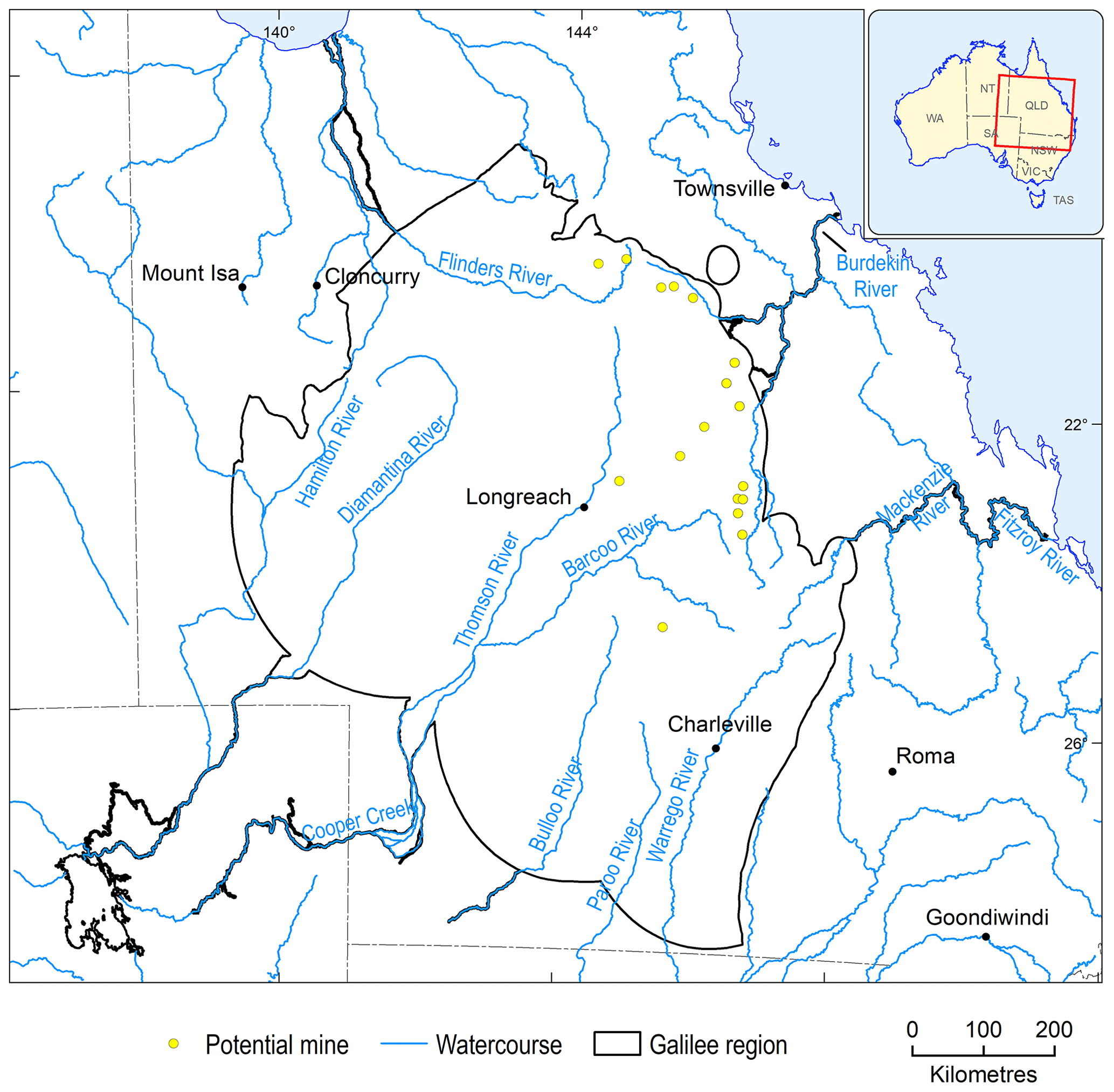
Figure 3 The Galilee region study area, showing the potential coal resource development sites.

The Galilee region includes the headwaters of seven major drainage catchments. These catchments are the Bulloo, Burdekin, Cooper Creek, Diamantina, Flinders, Paroo and Warrego. The largest of these catchments within the region are Cooper Creek and Diamantina. Groundwater within the region is a very important resource, as most of the streams are ephemeral. Groundwater is used for town water, agriculture and industry. Most groundwater in the region is extracted from the Great Artesian Basin.

The region covers a range of environments, including the mountains of the Great Dividing Range in the east through to semi-arid and arid areas in the central and western parts of the region. The main land use in the region is livestock grazing on native vegetation. There is no intensive agriculture in the region and a low human population density, largely due to the low and unpredictable rainfall (Evans et al., 2014).

2.1.3 Maranoa–Balonne–Condamine region

The Maranoa–Balonne–Condamine region covers approximately 130 000 km² and is located mostly within south-east Queensland with about half of this area within the Murray–Darling Basin. From east to west, average annual rainfall decreases from 800 to 420 mm, while PET increases from 1500 to 2370 mm. The region overlies the Surat Basin and has five open-cut coal mines and five CSG projects, as well as two proposed open-cut coal mines (Fig. 4).

Figure 4 The Maranoa–Balonne–Condamine region study area, showing the potential coal resource development sites.

The region contains the headwaters of the Condamine–Balonne, Moonie, Weir, Maranoa and Dawson rivers. Most of the rivers within the region are ephemeral. Therefore, groundwater is an important water source and is used for stock and domestic purposes as well as, in some cases, town water supply. The Great Artesian Basin is the main source of groundwater used within the region (Welsh et al., 2015).

The main land use within the region is grazing on natural vegetation, with dryland cropping and production forestry also being major land uses. The main vegetation type within the region is grassy woodlands, with river red gums, coolabah and river oak common riparian species. There are also six wetlands of national significance within the region: Balonne River Floodplain, Boggomoss Springs, Dalrymple and Blackfellow Creeks, Lake Broadwater, Palm Tree and Robinson Creeks, and The Gums Lagoon (Welsh et al., 2015).

2.2 Landscape classification development – overview and rationale

The purpose of this ecohydrological landscape classification is to characterise the landscape based on patterns in land use, ecology, geomorphology and hydrology and, from these, to develop landscape classes of water-dependent, remnant and human-modified features. We chose these features because these three types represent a generally applicable delineation for classification development in our different regions. For example, in Australia, remnant vegetation (our remnant features) describes all vegetation where there was no clearing or regrowth of (semi-) native vegetation, resulting in a vegetation community that resembles its predecessor's structure. It represents areas with low to very minimal human interference. This is opposed to human-modified sites, at which human activities are the defining features of the area, such as urban areas or other infrastructure. Water dependency is essential for establishing a conceptual linkage of water across landscape elements. Our classification employs a geographical information system to overlay existing spatial data for each region. The spatial data are the basis for categorising the landscape features using a rule set to prioritise the spatial data based on their attribute features.

The datasets have a regional, state or national coverage. Using a feature-based classification helps to place the landscape classes within a common biophysical system that aids in formulating conceptual models and patterns in water dependency across the landscape of each region. This provides a classification that is aligned with the idiosyncrasies of each region. Maintaining regionality is essential when developing conceptual models and quantitative models for assessing the risk to ecological components from hydrological changes. For example, arid and semi-arid regions have very different ecological environments, functions and processes compared with subtropical or temperate woodlands.

Our approach uses a defined rule set and priorities, which we apply to regionally available datasets to achieve a landscape classification for each of our regions. Tables 1–3 provide a list of citations for example datasets used in this process. This is different from most other landscape classifications that may use climate, topography, hydrological assessment units and remote-sensing data and apply statistical dimensionality reduction and classifications, such as proximity analysis (e.g. Gharari et al., 2011; Leibowitz et al., 2014; Sawicz et al., 2014; Zhang et al., 2016; Addicott et al., 2021; Carlier et al., 2021; Jones et al., 2021).

Table 1 Landform classification criteria and example datasets.

^* NSW: New South Wales.

Table 2 Stream classification criteria and example datasets.

Table 3 Spring classification criteria and example datasets.

When considering the characteristics of our regions, the following features form part of the rule set for defining landscape classes:

• road habitat/land use type (remnant/human-modified);

• wetland (wetland/non-wetland);

• topography (upland/lowland, floodplain/non-floodplain);

• groundwater (groundwater-dependent/non-groundwater-dependent, Great Artesian Basin (GAB)/non-GAB) (note: identifies groundwater dependency and classifies this with the presence/absence of Great Artesian Basin groundwaters);

• vegetation type (riparian/woodland floodplain/grassy woodland/rainforest);

• water regime (permanent/ephemeral/null) of surface water.

These features identify groups of landforms and use streams and springs.

The hydrological connectivity is the main reason for developing a new classification, as this allows us to assess the potential impact of coal resource developments on the landscape via a water pathway. Therefore, the most important characteristics are the hydrological features. Describing the conceptual understanding of how water connects the landscape elements allows us to identify where in the landscape impacts are likely to occur. In line with this, we developed a hierarchical approach, in which hydrological features have priority over other landscape characteristics. This resulted in a spatially complete landscape classification, in which there are no gaps in the mapping data. The method of prioritisation depended on region-specific characteristics and the data availability. This yielded a classification in which the landscape classes have their origin in the spatial datasets, and it included the water dependency, which was a prerequisite for the prioritisation. An example prioritisation assigned in order of highest to lowest is as follows:

• aquatic ecosystems (e.g. wetlands, streams and lakes);

• remnant vegetation;

• other landscape components that are non-remnant vegetation and are typically anthropogenically modified.

Subsequent use of the landscape classification for risk identification with expert input also required the combination of landscape classes into broader landscape groups. Landscape groups are sets of landscape classes that share ecohydrological properties. These landscape groups provided efficiencies in the expert elicitation process of the risk modelling, as they combined similar ecological system components based on our landscape classes while also accounting for region-specific differences. For example, in the Namoi region there are two landscape groups where we do not expect any impact from coal resource developments. Firstly, the Dryland remnant vegetation landscape group is ruled out with respect to potential impacts because it comprises vegetation communities that are reliant on incident rainfall and local runoff and do not include features in the landscape that have potential hydrological connectivity to surface water or groundwater features. Secondly, the Human-modified landscape group is excluded from the ecological impact assessment because it primarily comprises agricultural and urban landscapes that are highly modified by human activity. Here, the impact assessment focus is on economic assets such as groundwater bores, and therefore beyond the scope of this publication.

2.2.1 Landform classification

Landform classification relied on the dominant land type of either habitat or land use to determine landscapes that are relatively natural and those that have been anthropogenically modified. Relatively intact areas are more likely to contain ecological assets, such as species and ecological communities, than highly modified areas. Location within the region (topography – upland/lowland, floodplain/non–floodplain), groundwater dependency and water regime were part of classifying the landscape. Determining areas that are subject to flooding or that have persistent water assists in identifying landscapes that support water-dependent habitat and vegetation as well as aquatic ecosystems (Table 1).

2.2.2 Stream classification

Stream classification in each of the study regions was based on stream position within the catchment (e.g. upland/lowland), water regime (perennial/near-permanent or ephemeral/temporary), and dependence and source of groundwater (Table 2). Catchment position is a potential indicator of stream morphology and flow patterns, while water regime is important when considering habitat suitability and physical processes within the channel and riparian zone. Streams can also gain and lose water to local and regional groundwater systems, interacting with groundwater-dependent ecosystems (Table 2).

2.2.3 Spring classification

The water source is the basis of spring classification. The source of groundwater is important when considering regional-scale landscape classifications, due to the hydrological connectivity of aquifers and potential coal resource developments (Table 3).

Figure 5 Overview of the Namoi landscape classification schema, including criteria and attributes resulting in six landscape groups.

3 Results

Below, we present the resulting landscape classes for the three regions. For each region, we also combined the landscape classes into landscape groups, which were specific to each region and were based on distinctions in topography, water dependency and association with Great Artesian Basin (GAB) or non-GAB groundwater-dependent ecosystems (GDEs), floodplain/non-floodplain or upland/lowland environments, and remnant/human-modified habitat types. The purpose of the landscape groups was to combine non-water-dependent landscape classes and relate water-dependent landscape classes to region-specific aspects of their water dependency. This enabled experts to develop a conceptualisation of the landscape for developing their ecological impact models. While the approach to defining the landscape classes is based on a consistent rule set and prioritisation, each of the regions has different landscape classes, which is a consequence of the differences in location, jurisdictions and available spatial datasets.

The rule set originating from the landform classification (Tables 1–3) and prioritisation of hydrological features is the main outcome of our approach, and we present the rule set as a decision pathway in Fig. 5. For example, for the Namoi region, the rule set includes the following: (1) identify the habitat (e.g. stream), (2) select by topography (e.g. upland), (3) identify the groundwater associations (e.g. GDE) and so on until one derives at the final landscape class level (see Fig. 5).

3.1 Landscape classes in the Namoi region

There were 29 landscape classes within 6 landscape groups in the Namoi region (Fig. 5). Of these landscape groups, Human-modified (non-remnant) was the largest (59.3 %; Table 4) and included urban, agriculture, plantations and other intensive land uses. Dryland remnant vegetation was the second largest landscape group and consisted of the Grassy woodland landscape class (24.2 %; Table 4). This landscape class was considered non-water-dependent because it did not intersect with floodplain, wetland or GDE features. The Rainforest landscape group was the smallest (0.5 %; Table 4), with only a limited distribution (Fig. 6a).

Table 4 Percentage of area of each landscape group for the Namoi region.

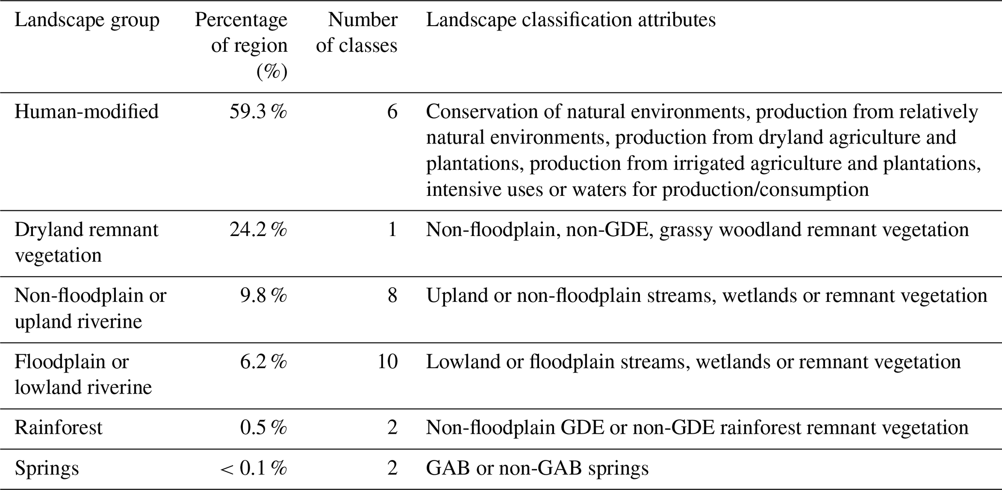
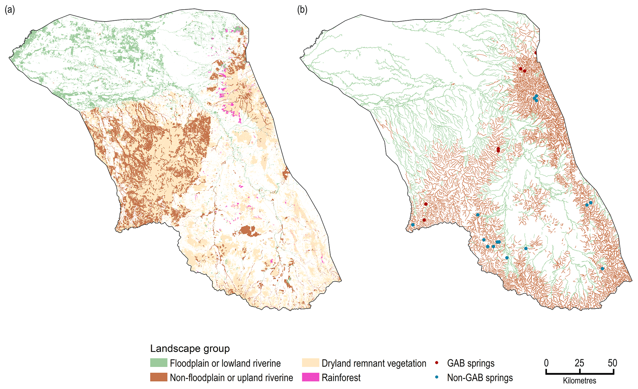
Figure 6 (a) Landscape groups (excluding the Human-modified group), and (b) stream network classified as Upland or Lowland in the landscape classification and Springs within the Namoi region. GAB: Great Artesian Basin. Data: Bureau of Meteorology (2012) and Bioregional Assessment Programme (2017).

The stream network consisted of two landscape groups (Floodplain or lowland riverine and Non-floodplain or upland riverine). The Non-floodplain or upland riverine landscape group had a larger proportion of stream network length (63.8 %) compared with the Floodplain or lowland riverine landscape group (36.2 %; Fig. 6b). There were 22 springs identified within the Namoi region, with 7 of these associated with the GAB (Fig. 6b).

Figure 7 Landscape classification of the Galilee region.

3.2 Landscape classes in the Galilee region

The Galilee region has 31 landscape classes organised into 11 landscape groups (Fig. 7). The Dryland landscape group was the largest group within the region and the only group to have no water dependency (68.5 %; Table 5). The landscape groups that covered the floodplain areas were the next most dominant classes: Floodplain, terrestrial GDE (12.94 %; Table 5) and Floodplain, non-wetland (11.8 %; Table 5). The remaining three non-floodplain landscape groups consisted of Non-floodplain disconnected wetlands; Non-floodplain, terrestrial GDE; and Non-floodplain, wetland GDE (4.9 % combined; Table 5).

Table 5 Percentage of area of each landscape group for the Galilee region.

The stream network was classified as groundwater-dependent or non-groundwater-dependent systems. Most of the streams in the region were non-GDEs (87.7 % compared with 12.3 % for the Streams, GDE landscape group). There were also over 3000 springs in the region.

3.3 Landscape classes in the Maranoa–Balonne–Condamine region

The landscape classification for the Maranoa–Balonne–Condamine resulted in 34 landscape classes within 5 landscape groups (Fig. 8). The largest landscape group was the Human-modified group (72.2 %, Table 6), which included agricultural production, plantations and other intensive land uses. Of the remaining landscape groups, Dryland remnant vegetation was the second most dominant (19.8 %, Table 6). It was not considered water-dependent, as it did not intersect with floodplain, wetland or GDE features.

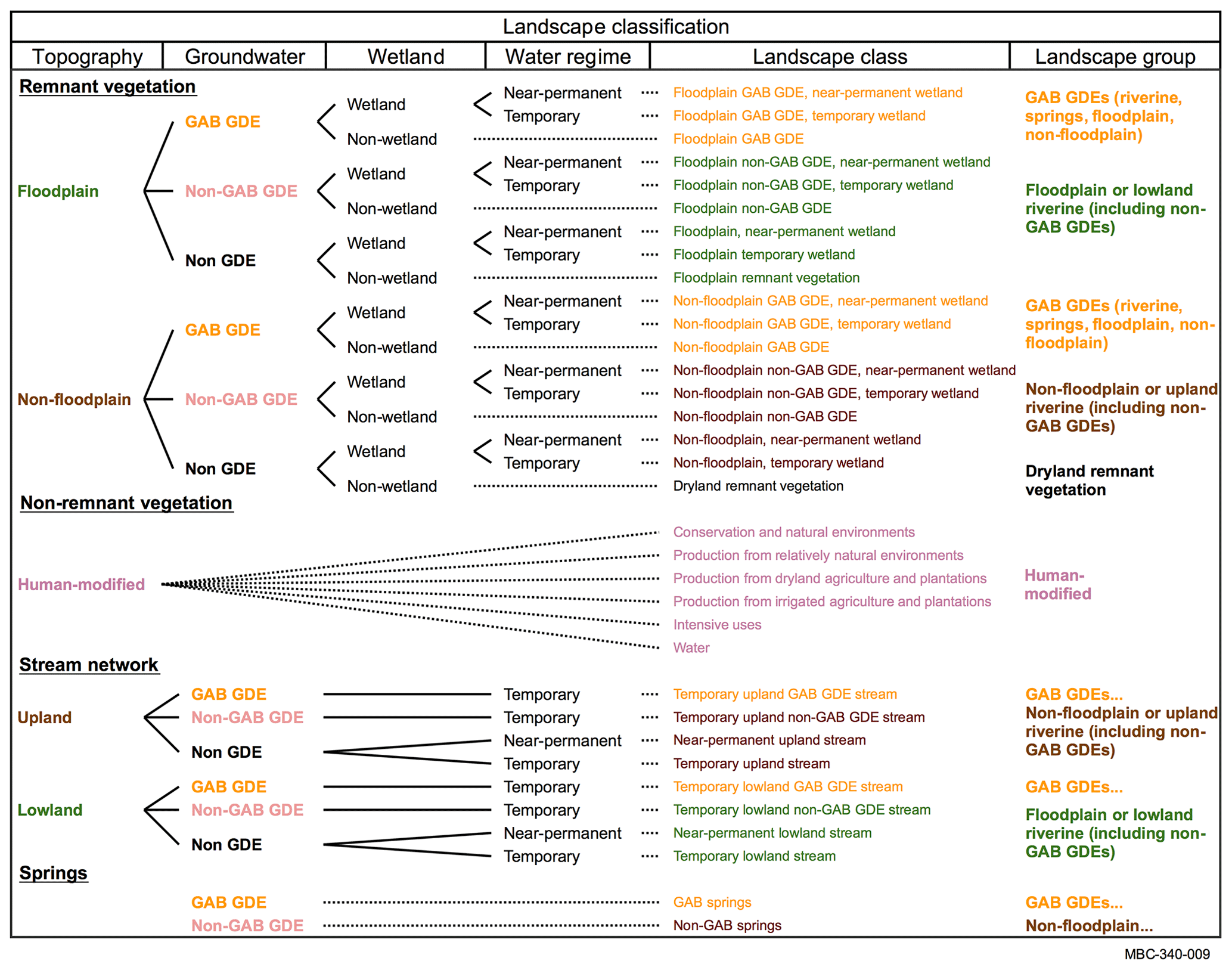
Figure 8 Landscape classification of the Maranoa–Balonne–Condamine region. GAB: Great Artesian Basin; GDE: groundwater-dependent ecosystem; GAB GDEs …: GAB GDEs (riverine, springs, floodplain, non-floodplain); Non-floodplain …: non-floodplain or upland riverine (including non-GAB GDEs).

Table 6 Percentage of area of each landscape group for the Maranoa–Balonne–Condamine region.

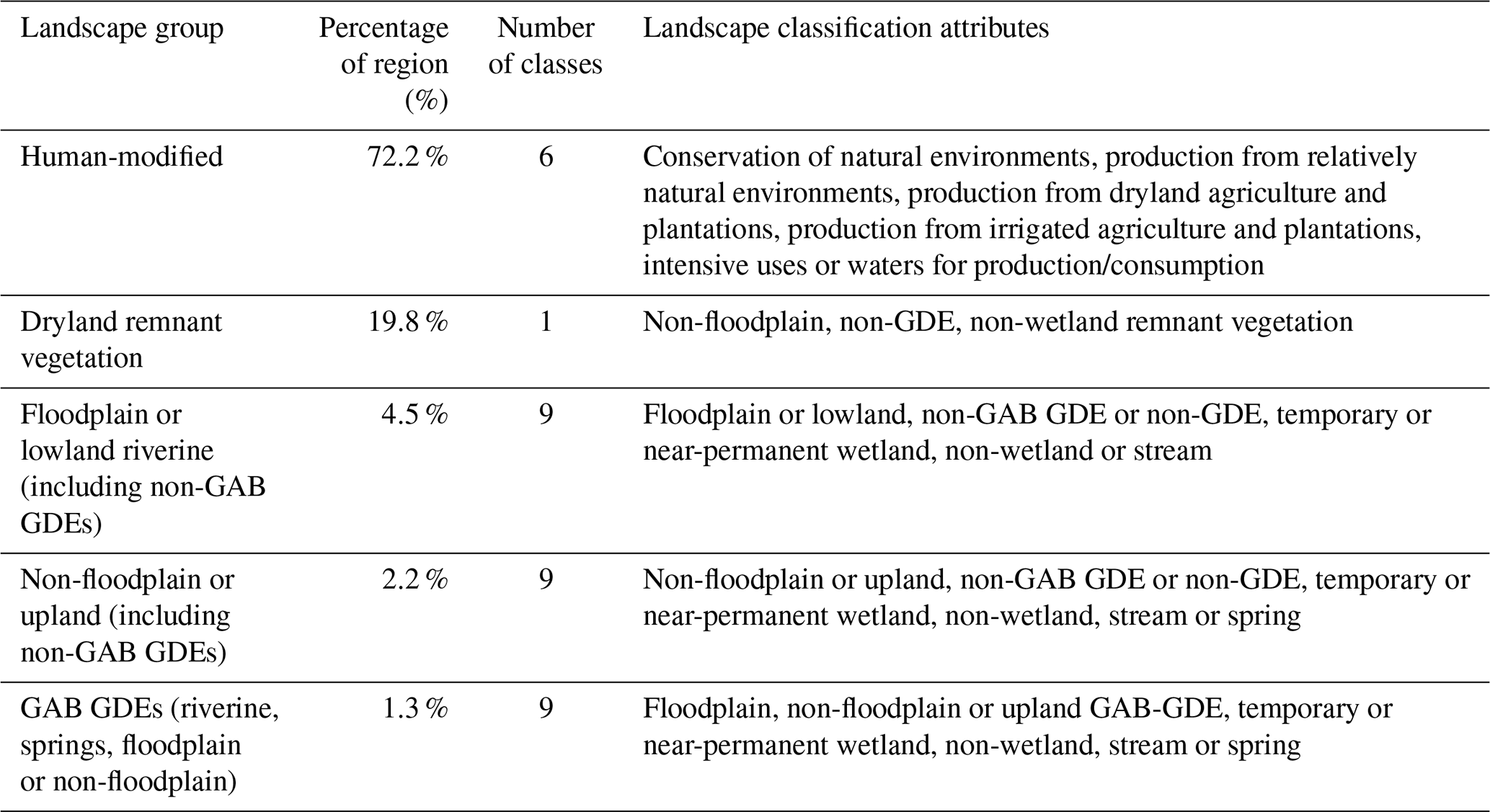
GAB: Great Artesian Basin; GDE: groundwater-dependent ecosystem.

There were three landscape groups that cover the stream network. The most dominant landscape group was Floodplain or lowland riverine (including non-GAB GDEs) (47.8 %), followed by Non-floodplain or upland riverine (including non-GAB GDEs) (39.4 %) and GAB GDEs (riverine, springs, floodplain or non-floodplain) (12.7 %). There were 177 springs identified within the region. Most of the springs were GAB GDEs (riverine, springs, floodplain or non-floodplain) (86.4 %, compared with 13.6 % for Non-floodplain or upland riverine (including non-GAB GDEs)).

4 Application of the landscape classification to the assessment of ecosystem risk

Here, we show an application of our classification approach. It presents the potential impact that coal resource developments can have on ecology using the Namoi region as an example, thereby demonstrating the useability of our classification approach.

The purpose of developing the landscape classification was to assess the risk of coal resource development with respect to the ecology of a region via a water pathway. Our landscape classification provided the spatial framework on which experts could base their assessment of risk from coal resource development to the ecology of a region. Details of the predicted changes in surface water and groundwater for the Namoi and Galilee regions are given in Post et al. (2020). Here, we demonstrate the assessment of potential ecological impacts using the Namoi region. For full details of the analyses in each of the three regions, readers are referred to Holland et al. (2017), Herr et al. (2018b) and Lewis et al. (2018). The models needed to identify water-mitigated linkages between hydrological changes, ecosystem components and the landscape classes. We briefly describe the expert assessment approach in a three-step process below.

The following describes an application of the landscape classification (see also Fig. 1); in doing so, we demonstrate that the classification is well suited for assessing the potential ecological impact of predicted surface water and groundwater changes. The three-step process illustrates the utility of our landscape classification approach with resect to assessing the risk to ecosystems. The process included experts identifying risk to landscape classes using their knowledge on local ecosystems within the landscape classes. Specifically, the experts used the broad landscape groups and their underlying hydrogeological features to develop initial qualitative models about priority ecosystem components. These then fed into building quantitative models. Here, the experts used outputs from surface water and groundwater modelling. This hydrological modelling identified the potential changes in water, which experts used to reach a consensus on what impact these changes may have on ecological entities within the landscape classes and/or groups. These agreed impacts fed into quantitative models that outlined the future hydrological changes and risks to the ecosystems in the landscape groups (see also Fig. 1).

Table 7 Upland riverine ecosystem quantitative modelling variables that experts prioritised in the qualitative model and associated ecological and hydrological variables used in the development of the quantitative impact model (after Ickowicz et al., 2018).

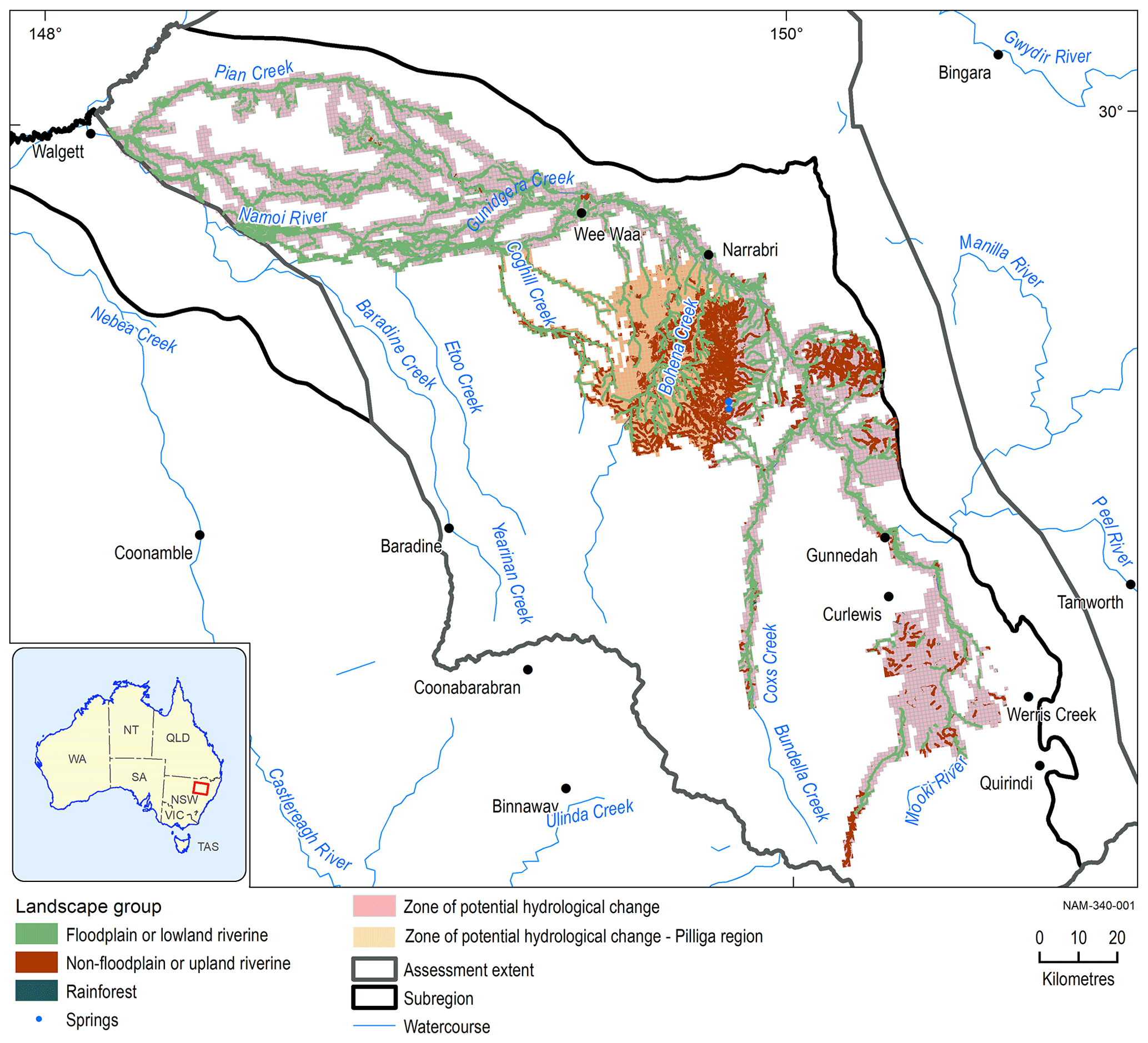
Figure 9 Landscape classes overlaying areas of potential hydrological change (Herr et al., 2018b).

Figure 10 Hydrological change risk level of lowland landscape class areas (Herr et al., 2018b).

Here, we use the example of the upland riverine landscape class in the Namoi region to outline the three-step process:

• Step 1 – develop qualitative models to conceptualise and prioritise ecosystem components of each landscape class and their linkage to hydrological variables.

  A qualitative model for the upland riverine landscape class agreed with the existing understanding that a reduction in overbank flows and lowering of the water table resulted in a reduction in several ecosystem components, including riparian habitat, amphibians and fish, and an increase in fine particulate matter, dissolved organic matter and cyanobacteria (Holland et al., 2017; Herr et al., 2018b; Hosack et al., 2018). A qualitative model has, at its basis, the conceptual understanding of ecosystem components and the direction of their interactions – that is, a positive, negative, or neutral influence of one component on another. This understanding also incorporates feedback loops between the ecosystem components in the form of sign-directed graphs, and it enables time-intensive quantitative model development to be directed at variables with the highest importance. The method is based on a matrix-level analysis of the component interactions (e.g. Herr et al., 2016; Ickowicz et al., 2018).

  In the process of building a qualitative model, the experts developed a consensus on the overall scope of the model, namely the model components and their interactions. The hydrological variables and the relationships between ecosystem components that the experts prioritised in the qualitative modelling process were the macroinvertebrate responses to riverine system change, presence of tadpoles and changes in projected foliage cover in the riparian trees along the stream channel (Table 7).

• Step 2 – use qualitative model priorities to develop quantitative models.

  In this context, qualitative models highlighted critical relationships and variables that became the focus of the quantitative models (e.g. Herr et al., 2016; Hosack et al., 2018; Ickowicz et al., 2018). The focus of the quantitative models was on three elements within the upland riverine landscape classes (Table 7). These three elements were (i) the response of upland riparian trees to changes in groundwater, (ii) macroinvertebrate assemblage changes related to days with no consecutive water (zero-flow days) and the longest zero-flow-event period, and (iii) the response of tadpoles to zero-flow days and the longest zero-flow-event period. Table 7 provides a brief summary of these variables; specific details of the variable definitions are given in Ickowicz et al. (2018).

• Step 3 – identify risk areas in the regions where quantitative modelling indicated significant changes to landscape group components.

  This quantitative modelling approach incorporated expert elicitation in a Bayesian framework to predict changes in ecological system components because of expected changes in hydrology conditions. The method dealt with complexity and with limited knowledge that allows for updates with new information, which is an important feature in evidence-based decision-making (e.g. Hosack et al., 2017).

  The modelling of risk to ecosystems at a regional scale focusses on recognising which parts of the region are potentially impacted and which parts are unlikely to experience harm. Using our landscape classification as a crucial input, the modelling delineated impacted areas within each region, based on a zone of potential hydrological change. This is the area in the landscape where hydrological modelling identified an expected change to surface water and groundwater from future resource extraction. Risk levels across a landscape group are a result of aggregating individual risks associated with each ecological variable and categorising the risks into three levels based on their percentile spreads (for details, see Herr et al., 2018b).

  For the Namoi region, for example, dryland remnant vegetation, human-modified ecosystems, non-floodplain and upland riverine ecosystems, and rainforests will not experience impacts, whereas floodplain and lowland ecosystems and streams or floodplain and lowland ecosystems will potentially experience impacts (Herr et al., 2018a). Figure 9 shows the landscape groups that are at risk of impact from hydrological changes because they are situated within the zone of potential hydrological change, while Fig. 10 shows the risk level to these landscape groups from the quantitative models. Note that there is a “Remaining unquantified `floodplain and lowland riverine' classes” category. The expert could not develop quantitative models for these classes, as there was no surface water hydrological model available that could predict changes to surface water flows. This was related to the lack of gauging data and groundwater interaction details specific to the lowland drainage channels. Having lowland riverine classes whose risk remains unquantified means there is additional work needed before assessment and potential mitigation of impacts from hydrological changes are possible (Herr et al., 2018b).

5 Discussion

In Australia, there is no consistent national classification that links ecosystems at the landscape level with their underlying hydrological system. While there are many different land classifications that incorporate hydrological aspects, they do not provide linkages between hydrology and landscape elements. None of these enable a broad-scale ecological assessment of impacts associated with changes in water flow and availability, and they are not sufficiently generic for the purpose of assessing landscape-level water-related impacts on ecosystems in a spatially explicit manner (Kilroy et al., 2008; Elmore et al., 2003; Brown et al., 2014; Liermann et al., 2012; Doody et al., 2017; Poff et al., 2010; Aquatic Ecosystems Task Group, 2012; Olden et al., 2012; Gharari et al., 2011). However, the Bioregional Assessment Program needed to assess the impacts of coal resource developments on ecological systems via a water pathway. Hence, we developed an ecological landscape classification that would be applicable to the markedly different assessment regions.

We developed this classification based on existing datasets that were readily available in the areas of interest. This is a much more resource- and time-efficient process then gathering new data using techniques such as remote sensing and taking hydrological measurements (e.g. Gharari et al., 2011; Leibowitz et al., 2014; Sawicz et al., 2014; Zhang et al., 2016; Addicott et al., 2021; Carlier et al., 2021; Jones et al., 2021). The latter would also have required intensive methodology development and would, in our opinion, not have provided fit-for-purpose information for the expert elicitation process. The advantage of our approach was that it integrated the relationships between water in the landscape and the landscape classes from the multiple dimensions in the input datasets, which allowed experts to develop causal reasoning. This causal relationship would have been much less clear when using dimensionality reduction and classifications such as proximity analysis, as such methods do not infer causality without external information.

Our classification identifies the causal pathways between the water dependency of its components and human activities that result in hydrological changes. Prioritising hydrological features ensures that there is a conceptual linkage between hydrology and landscape classes, as it identifies ecohydrological landscape elements. This was crucial for the experts' understanding of how hydrological changes impact the landscape. No currently existing ecohydrological classification was suitable to do this, either because the classification was not spatially explicit or it did not cover the landscape completely (Poff et al., 2010; Aquatic Ecosystems Task Group, 2012; Olden et al., 2012). A spatially complete coverage of the landscape is an important prerequisite for the risk analysis because it enables the assignment of risk levels to the whole landscape and allows one to identify parts of the landscape where there is insufficient information from the other modelling components. In time-critical environmental impact assessments, developing models of different environmental elements often occurs in parallel for those areas where data are available. Where data are unavailable, such modelling is left for future work to improve the risk assessment. In our case, as we had a complete spatial coverage of the landscape, we could pinpoint the parts of the risk modelling inputs where we needed to prioritise further work. This identified the areas where hydrological modelling needed further refinement because of the lack of gauging stations and knowledge of surface water–groundwater interactions in some of the lowland drainage channels (Fig. 10).

While our spatially explicit landscape classification provided experts with the ability to readily identify cause-and-effect relationships between landscape elements and landscape hydrology, there are obvious differences between the landscape classifications in the three regions, reflecting their geographical differences (see Figs. 5, 7 and 8). This provides the specificity that is required in a regional impact assessment, where the boundaries are based on a combination of geology, water resources and administrative conditions. The regionality also means that there is need for different datasets describing the landscape features that would not be available from a single national classification covering the whole of Australia.

Nevertheless, each landscape classification provides a typology with an explicit connection of water to the landscape class. This connection enables a causal link between hydrological change and impact to ecosystems represented by landscape classes. The causal linkage is dependent on (i) a spatially explicit connection between water in the landscape and the landscape classes, (ii) a conceptual understanding how changes in water may result in a reaction of specific ecosystem elements in the landscape class and/or landscape group, and (iii) a way of modelling quantitative changes in ecosystem elements related to changes in water that incorporates causality. Our ecohydrological classification approach for landscapes provides this spatially explicit connection and has implicit ecohydrological elements that foster the conceptual understanding of the causal linkage. For example, spatially modelling groundwater-level drawdown enables a prediction of which springs may be experiencing impacts from water extraction and, with additional modelling, by how much and when. Linking this information with ecological expert inputs will then allow for the identification of impacts on the spring communities and the risk to the communities.

Subsequent ecological modelling using expert elicitation of potential impacts drew heavily on our classification, which is based on a consistent rule set and fosters conceptual understanding of landscape processes and functions. It provides an essential framework for experts to understand and conceptualise how modelled future hydrological changes from coal resource developments link to potential ecological changes at the landscape level. It is the basis for modelling the ecological risk to the landscape from hydrological changes, and it allows for the incorporation of different data sources and existing classification schemes. This consistency makes the classification development transparent, repeatable and adjustable, should new data become available.

5.1 Limitations

While the ecohydrological landscape classification approach provided the basis for the risk assessment outlined above, there are some limitations that require consideration when attempting to develop and apply this ecohydrological landscape classification approach.

An important issue for the landscape classification is formulating a typology that adequately reflects both the functional and structural complexity of the ecosystem. At the same time, it also needs a succinct and consistent representation of the system that is “fit for purpose”, which in our context means showing a hydrological connectivity between the landscape classes as well as within the general landscape. The systematic classification imposes discrete boundaries among landscape components that may not adequately capture gradients within and across landscape classes. This approach tends to simplify important components of ecotones such as “transition” zones or edges between landscape classes, where ecosystem processes and/or biodiversity are likely to peak and tensions between human-induced boundaries occur (Ward et al., 1999; Ryberg et al., 2021). If landscape classes are treated purely as “closed” ecosystems, then the result may be a poor representation of the biotic interactions and energy exchange between adjacent systems, and this could limit a conventional impact and risk analyses. These conceptual challenges may be important considerations for subsequent impact assessments, requiring special attention in assigning risk from human-induced changes in hydrology. However, expert modelling of impacts can compensate for this shortfall, when, for example, incorporating riparian areas in riverine and wetland impact model development. In our case, experts intrinsically applied the ecotone concept to riparian areas when discussing and assigning impacts to stream ecosystem variables, thereby overcoming the tension of boundaries that the classification imposed (see also Hosack et al., 2018; Ickowicz et al., 2018).

There are also spatial data issues that require additional consideration beyond just simply incorporating existing data. There are several technical issues that constitute important gaps in the landscape classification for the Namoi region, for example. Here, two different approaches to define GDEs were required because one spatial dataset only included terrestrial vegetation and not riverine systems mapped within the stream network (NSW Office of Water, 2015). A second GDE dataset helped overcome this deficiency and provided the basis to classify the stream network's dependency on groundwater (Bioregional Assessment Programme, 2012).

Wetlands in large areas of Australia have not yet been adequately mapped. The separation between groundwater-dependent and surface-water-dependent wetlands may not always be accurate. In many areas, there is little knowledge of groundwater–surface water interactions. There is also a significant gap in the understanding of water thresholds for ecosystems associated with springs. In part, this results from a lack of bores to provide meaningful groundwater data. Some examples of these data gaps appear in the discussion of the functioning of springs in the Doongmabulla Springs complex in the Galilee region, particularly with respect to identifying the source aquifer (Fensham et al., 2016).

There is extensive work from Queensland that links regional ecosystems' vegetation to their groundwater needs, although the mapped areas are still small (Sattler and Williams, 1999; Queensland Government, Queensland, 2016; Queensland Herbarium, 2021). However, in many parts of Australia, GDE mapping and classification approaches are limited and many areas lack systematic ground-truthing. This is especially true in areas with extensive intact native vegetation remnants, such as the Pilliga Forest of the Namoi region, where large areas of the Grassy woodland GDE landscape class exist, but a lack of published studies on vegetation–groundwater interactions limits a definition of the nature of this interaction. This is where a risk approach can compensate for the lack of knowledge, as an elevated assigned risk can reflect the limits in understanding.

5.2 Conclusions

We showed that our landscape classification approach worked in the three geographically different regions, with widely disparate information sources that fed into a landscape classification. This also results in a resource-efficient approach, as existing spatial landscape or ecosystem classification schemes, developed for other purposes, can be incorporated into the classification.

The study was able to formulate and implement an attribute-based classification scheme to define and delineate water-dependent features across three large regions. We conclude that this approach allowed us to repurpose several existing schemas into an adaptable and practical typology of a landscape classification. The conceptual framework of landscape ecohydrology forms the basis for this classification, which is used to focus subsequent analysis of potential cumulative impacts on water resources from multiple coal resource developments. The classification enabled the development of specific conceptual and quantitative models that linked changes in hydrology to potential impacts on ecosystems using the landscape classes. The classification provided crucial inputs for a risk analysis of landscape components subject to hydrological changes.

Applying our approach to different regions showed that it is sufficiently general and flexible to enable the development of ecohydrological classifications in regions in Australia and potentially in other regions around the globe, given a sufficiently mature information base and data availability.