A high-resolution map of diffuse groundwater recharge rates for Australia

Estimating groundwater recharge rates is important to understand and manage groundwater. Numerous studies have used collated recharge datasets to understand and project regional- or global-scale groundwater recharge rates. However, recharge estimation methods all have distinct assumptions, quantify different recharge components and operate over different temporal scales. We use over 200 000 groundwater chloride measurements to estimate groundwater recharge rates using an improved chloride mass balance (CMB) method across Australia. Groundwater recharge rates were produced stochastically using gridded chloride deposition, runoff and precipitation datasets. After filtering out groundwater recharge rates where the assumptions of the method may have been compromised, 98 568 estimates of recharge were produced. The resulting groundwater recharge rates and 17 spatial datasets were integrated into a random forest regression algorithm, generating a high-resolution (0.05°) model of groundwater recharge rates across Australia. The regression reveals that climate-related variables, including precipitation, rainfall seasonality and potential evapotranspiration, exert the most significant influence on groundwater recharge rates, with vegetation (the normalised difference vegetation index or NDVI) also contributing significantly. Importantly, the mean values of both the recharge point dataset (43.5 mm yr⁻¹) and the spatial recharge model (22.7 mm yr⁻¹) are notably lower than those reported in previous studies, underscoring the prolonged timescale of the CMB method, the potential disparities arising from distinct recharge estimation methodologies and limited averaging across climate zones. This study presents a robust and automated approach to estimate recharge using the CMB method, offering a unified model based on a single estimation method. The resulting datasets, the Python script for recharge rate calculation and the spatial recharge models collectively provide valuable insights for water resource management across the Australian continent, and similar approaches can be applied globally.

1 Introduction

Groundwater is a critical component of the water cycle, providing baseflow to streams and supporting ecosystems and livelihoods (Brunke and Gonser, 1997; Eamus, 2006; Shah, 2005). With impacts from climate change, population growth and increased usage, groundwater resources are expected to become even more important in the future (Döll, 2009; Famiglietti, 2014; Wada et al., 2010), requiring a detailed understanding of hydrogeological processes through desktop studies, numerical modelling and direct field measurements. Assessing groundwater resources requires not only understanding their distribution, natural discharge and extraction rates but also understanding mechanisms and rates of resource replenishment.

Groundwater recharge is one of the most important, albeit challenging, components to quantify in groundwater assessments due to its wide spatiotemporal variability, which is influenced by a range of geo-eco-climatic factors (de Vries and Simmers, 2002). Recharge estimation is further complicated by the conceptualisation of recharge mechanisms (e.g. diffuse versus focused; Lerner et al., 1990). Similarly, the uncertainties in recharge estimation techniques provide further challenges (Scanlon et al., 2002). Additional complexities need to be carefully considered in recharge studies, including understanding the timescales associated with the technique(s) being used (e.g. Scanlon et al., 2002, and Cartwright et al., 2017) and the component of recharge being estimated (e.g. gross, potential or net recharge; Crosbie et al., 2010a).

Large-scale studies of groundwater recharge (e.g. global and continental scale) that are based on the compilation of recharge estimates typically utilise recharge estimates obtained from different techniques (e.g. Petheram et al., 2002; Scanlon et al., 2006; Crosbie et al., 2010a; Mohan et al., 2018; Moeck et al., 2020; MacDonald et al., 2021; and Berghuijs et al., 2022). These combined datasets allow an assessment of the changes in recharge rates over time due to climate variability or land cover change (e.g. Scanlon et al., 2006). However, such datasets add extra uncertainty to the predictive models that utilise them, given that they include recharge estimates with different assumptions, temporal scales and mechanisms (e.g. Crosbie et al., 2010a, and Mohan et al., 2018). Utilising different recharge estimation techniques may result in widely different recharge rates (e.g. Crosbie et al., 2010a; King et al., 2017; Walker et al., 2019; and Cartwright et al., 2020).

Selecting recharge estimates from a single technique from these global studies could overcome the issues mentioned above but could also lead to insufficient spatial coverage for meaningful continental-scale assessments. For example, the issue of spatial coverage of recharge estimates is evident in Australia from the sparseness of recharge estimates in the interior of Australia (e.g. Moeck et al., 2020, and Berghuijs et al., 2022). Studies in Australia have addressed the issue of data sparsity through creation of a series of empirical relationships between rainfall and recharge by investigating key factors such as vegetation and soil types (e.g. Crosbie et al., 2010a, and Leaney et al., 2011). More recent Australian studies have utilised statistical methods to investigate the influence of environmental variables on groundwater recharge (e.g. Fu et al., 2019) or have applied machine-learning techniques to predict future recharge (e.g. Huang et al., 2019, 2023). Others have focused on the upscaling of point estimates from a single technique (e.g. chloride mass balance) to a regular grid across regional study areas using regression kriging (e.g. Crosbie et al., 2018, 2022, and Crosbie and Rachakonda, 2021).

The chloride mass balance (CMB) method is one method that provides the opportunity for detailed studies of diffuse groundwater recharge rates, given the wide availability of groundwater chloride concentration measurements. The CMB method is also the most widely used recharge estimation technique globally (Moeck et al., 2020), in semi-arid and arid regions (Scanlon et al., 2006) and in Australia (e.g. Crosbie and Rachakonda, 2021; Crosbie et al., 2018, 2010a, b; and Petheram et al., 2002). The CMB method provides long-term estimates of diffuse recharge over the timescale required for chloride to accumulate in the subsurface, which ranges from years to decades in temperate settings (Cartwright et al., 2020) and up to thousands of years in semi-arid and arid areas (Scanlon et al., 2002, 2006). Spatially, the CMB method estimates diffuse recharge over the areas upgradient from the measurement location, ranging from a few hundred metres to several kilometres (Scanlon et al., 2002). Generation of chloride deposition maps (e.g. Davies and Crosbie, 2018, and Wilkins et al., 2022) has allowed for the large-scale (regional) use of the CMB method (e.g. Crosbie et al., 2018). Irvine and Cartwright (2022) utilised the chloride deposition maps from Davies and Crosbie (2018) to automate the application of the CMB method in Python. Automating the application of the CMB method provides opportunities for large datasets of recharge to be efficiently generated from chloride measurements.

This study utilises recently developed chloride deposition maps from Wilkins et al. (2022) and approaches to automate analyses to estimate long-term diffuse groundwater recharge rates based on the CMB method across the Australian continent. We collate a large dataset of groundwater chloride and associated spatial datasets to facilitate the recharge estimates. We utilise these datasets and the random forest algorithm to develop a regression model for long-term diffuse groundwater recharge rate estimation for the Australian continent. Using the model, we explore the control of environmental variables on groundwater recharge rates, quantify the uncertainty in recharge rate predictions, and produce point datasets and high-resolution gridded maps of diffuse recharge for Australia.

2 Methods

2.1 Collation of groundwater chloride dataset

Groundwater chloride measurements were collated from the following sources: the Geoscience Australia Portal (Geoscience Australia, 2022), the Commonwealth Scientific and Industrial Research Organisation (CSIRO) Hydrogeochemical Mapping of the Australian Continent series dataset (Gray et al., 2019; Gray and Bardwell, 2016a, b, c, d, e, f; Henne and Reid, 2021), a dataset collated for the state of South Australia (Broad, 2020), Visualising Victoria's Groundwater (FedUni, 2022) and a Northern Territory government isotope dataset (Steven Tickell, personal communication, 12 April 2022). The preliminary collated dataset contained a total of 226 954 chloride measurements (including bores with time series data and duplicate values). A breakdown of the individual counts of each dataset compiled is provided in Table S1 of the supporting information.

Bore log information was downloaded from the Australian Groundwater Explorer (Bureau of Meteorology, 2022b) to provide locations, bore hole depths, drilled depths and screened interval depths. The depth assigned to each chloride measurement was applied in the following order of preference: screen mid-point depth, sample depth, bore depth and hole depth. Measurements with no depth information were removed from the analyses.

Several preliminary measures were undertaken for quality assurance of the chloride data. All measurements without latitude and longitude were removed. Chloride measurements that were reported below the analytical detection limit (i.e. <1 mg L⁻¹) were removed from the dataset. All duplicates with matching bore identifiers, latitude and longitude (in decimal degrees), sample date, and chloride concentration were presented as a single measurement, resulting in 192 300 measurements. Measurements without a sample date were retained because excluding them would remove 99.8 % of measurements from the state of Western Australia (n=19 967).

Bores with repeat measurements from different sample dates were represented as the mean of the time series, producing a final dataset with 115 630 bores, each with a single chloride value for the analyses. Due to the size of the dataset, analysis of charge balance errors was not undertaken in this study. The final chloride dataset is provided as a downloadable electronic data file in the supporting information.

2.2 Collation of spatial datasets

To investigate factors that influence groundwater recharge, we identified 17 different spatial datasets – 16 of which are available as gridded maps (Table 1). These variables were chosen based on their use in previous global groundwater recharge studies (e.g. Mohan et al., 2018, and Moeck et al., 2020) or in regional-scale to continental-scale recharge studies in Australia (e.g. Crosbie et al., 2010a, and Leaney et al., 2011). All analyses in our study utilise the native resolution of the datasets shown in Table 1.

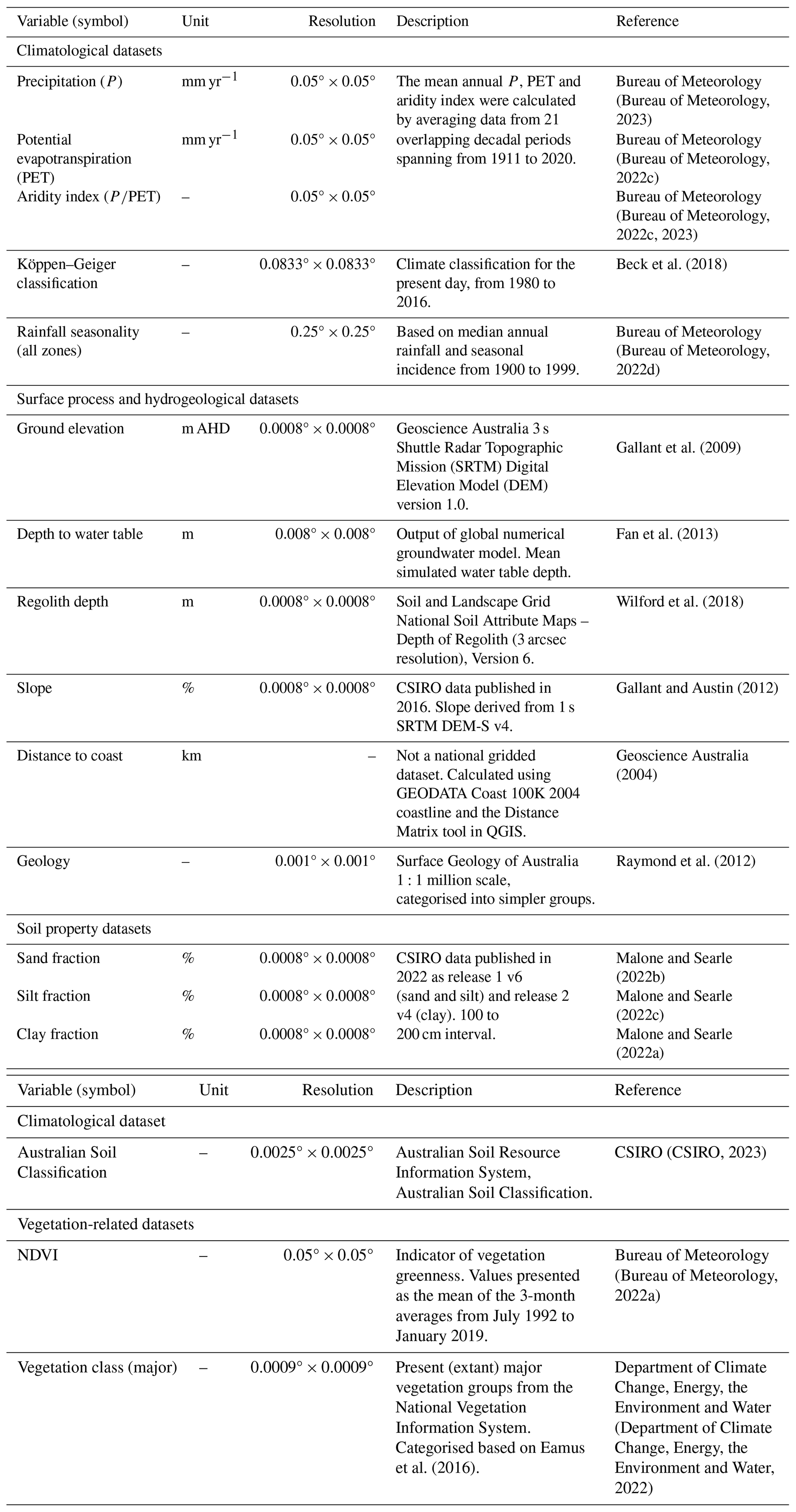
Table 1 Spatial datasets of factors that are known to influence groundwater recharge. Variables are grouped into climatological-related, surface-process- and hydrogeological-related, soil-property-related, and vegetation-related datasets. AHD denotes the Australian Height Datum.

The decadal rainfall maps from the Bureau of Meteorology (2023) were chosen over the Australian Water Outlook precipitation data (Bureau of Meteorology, 2022c) used in the Australian Water Resources Assessment Landscape (AWRA-L) model (Frost and Shokri, 2021) due to missing and unreliable data in the Australian Water Outlook dataset for a large area of north-central Western Australia and other smaller areas in South Australia and the Northern Territory. Non-gridded spatial data were also used, including the Australian coastline (Geoscience Australia, 2004; for the purposes of approximating the distance from bore holes to the coast; Table 1) and a halite deposit dataset of Australia (Feitz et al., 2019).

Spatial maps of the variables from Table 1 and the halite deposits are provided as Fig. S1 in the supporting information.

To assist with later assessments, all gridded spatial data collated in Sect. 2.2 (Table 1) were appended to the recharge output produced later in Sect. 2.3. The Point Sampling Tool in QGIS was used to extract the corresponding value from the raster pixel in which the groundwater recharge rate derived from CMB is located. The Distance Matrix tool in QGIS was used to measure the nearest distance to the Australian coastline. Some groundwater recharge rates were located outside of the extents of some gridded spatial data.

To produce a continental-scale recharge estimator, all spatial resolutions were converted to a 0.05° grid. For conversion, the GDAL Warp (reproject) tool in QGIS was used, utilising the average resampling method. The average resampling method was chosen as opposed to one of the more commonly used methods that take the value or aggregation of a limited number of the nearest pixels (e.g. nearest neighbour, bilinear interpolation or cubic convolution). The average resampling method considers all pixels that contribute to the output pixel in its calculation, preserving the overall statistical characteristics of the data while producing a smooth output (similar to cubic convolution) and covering areas of the coastline that were not observed using other resampling methods.

2.3 Chloride mass balance analysis

The CMB method produces estimates of long-term groundwater recharge by comparing groundwater (or soil water) chloride concentration to that measured in rainfall (and dry deposition), provided that various assumptions are met (Wood, 1999; Leaney et al., 2011). The method assumes that chloride acts conservatively, that chloride is solely sourced from precipitation and that groundwater has returned to steady-state conditions following any land-use changes (e.g. vegetation clearing; Leaney et al., 2011). Following Davies and Crosbie (2018), recharge (R; mm yr⁻¹) from the CMB method can be calculated using the following equation:

$$\begin{array}{}\text{(1)}& R={\displaystyle \frac{\mathrm{100}D}{{\mathrm{Cl}}_{\mathrm{gw}}}},\end{array}$$

where D is the chloride deposition rate due to rainfall (kg ha⁻¹ yr⁻¹), Cl_gw is the chloride concentration in groundwater (mg L⁻¹) and a multiplier of 100 is applied for unit conversion.

While Eq. (1). assumes that no chloride is exported laterally, the input and output of chloride through runoff or run-on can be accounted for by modifying Eq. (1) (e.g. Crosbie et al., 2018). Accounting for lateral export of chloride can be especially important in upland areas with steep topography and high rainfall (Leaney et al., 2011). The uncertainty associated with run-on is suggested to be negligible (e.g. Crosbie et al., 2018), while the uncertainty associated with chloride concentration in runoff is small compared to that of chloride deposition (Leaney et al., 2011). However, due to the large number of bores and the continental scale of this study where a range of landscapes may be covered, runoff was accounted for to address this uncertainty. Following Crosbie et al. (2018) and Crosbie and Rachakonda (2021), a modified version of Eq. (1) can be used:

$$\begin{array}{}\text{(2)}& R={\displaystyle \frac{\mathrm{100}D(\mathrm{1}-\mathit{\alpha }\cdot \mathrm{RC})}{{\mathrm{Cl}}_{\mathrm{gw}}}},\end{array}$$

where RC (–) is the runoff coefficient determined by dividing the long-term average annual runoff by the long-term average annual precipitation and α is a scalar.

In this study, we used a modified version of the Chloride Mass Balance Estimator of Australian Recharge (CMBEAR; Irvine and Cartwright, 2022). The modified version of CMBEAR utilises the Australian gridded dataset of chloride deposition (i.e. Wilkins et al., 2022) to automate recharge estimation using the CMB method. The modified version also applies Eq. (2) where the previous version applied Eq. (1). In this updated version of CMBEAR, when applying Eq. (2) uncertainty, each input variable is quantified using a stochastic approach adopted from Crosbie et al. (2018).

Out of 115 630 bores in our dataset, 79 % had only one groundwater chloride measurement available. To estimate an uncertainty in groundwater chloride, bores with more than 10 measurements (n=1516) were used to calculate a mean coefficient of variation (CVμ). As per Crosbie et al. (2018), the coefficient of variation was calculated for each bore, with the resulting CVμ as the mean of these values. The CVμ of 0.37 was multiplied by the mean chloride value (Cl_gwμ) for each bore in our dataset to estimate the standard deviation (Cl_gwσ). The Cl_gwμ and Cl_gwσ were then used to generate normal distributions for each bore. A normal distribution was adopted because 52 % of bores with more than 10 measurements passed a normality test (p value > 0.05). The approach of using the CV rather than using a standard deviation directly was made since the CV scales with the mean chloride value, whereas applying the same standard deviation to all values could be problematic for small values (i.e. values becoming negative).

For each bore, the mean, standard deviation and skew of the chloride deposition (Dμ, Dσ and D_skew, respectively) were extracted from the chloride deposition map in Wilkins et al. (2022) from the pixel in which the bore was located and were used to generate a Pearson type III distribution following the description from Wilkins et al. (2022).

While the RC extracted from the location of the bore is held constant, this value is scaled down by the α value (Eq. 2), which is sampled from a uniform distribution between 0.33 and 0.66. This scaling approach is adopted from Crosbie et al. (2018) to deal with uncertainty in the proportion of baseflow contributing to runoff and the below-average chloride concentration in high-intensity rainfall events that typically generate runoff. Long-term annual runoff was calculated by averaging annual runoff data from 21 overlapping decadal periods spanning from 1911 to 2020 (Bureau of Meteorology, 2023). As these runoff data were an output from the AWRA-L model (Frost and Shokri, 2021) and were reliant on precipitation inputs that contained missing and unreliable values (see Sect. 2.2), the runoff data were therefore unreliable in certain areas. The problematic areas were identified as those with long-term annual precipitation < 100 mm yr⁻¹; a dataset was created using these areas and was used to convert all RC values in problematic areas to 0.0018 (the minimum RC calculated for an adjacent rectangular area covering similar latitudes and longitudes, from −29.5 to −20.5° and from 133.0 to 136.0°, respectively, compared to the problematic areas). Long-term average annual precipitation was calculated from decadal rainfall maps (Bureau of Meteorology, 2023) as mentioned in Table 1. While further investigation into the range and distribution type for the α value could be conducted, the range used has been used across multiple climate zones (e.g. Crosbie et al., 2018, 2022, and Crosbie and Rachakonda, 2021).

A probability distribution was created for each bore by calculating recharge (R) 1000 times using the 1000 sampled replicates from the distributions of Cl_gw, D and α. To quantify the uncertainty in recharge estimates, the median recharge (R₅₀), 95th-percentile recharge (R₉₅) and 5th-percentile recharge (R₅) values were calculated from each probability distribution and provided as outputs for each bore. The median was chosen as it is unaffected by extreme outliers, as is not the case with the arithmetic mean.

2.4 Data filtering

The assessment of the suitability of input data for the application of the CMB method is a vital step to ensure that the assumptions of the method are met (Irvine and Cartwright, 2022). In our study, this assessment (hereafter referred to as “data filtering process”) involved six steps that were performed after obtaining the recharge estimates.

The data filtering process removed recharge estimates where the following conditions likely invalidate the CMB method or where unrealistic recharge estimates were produced.

1. Bores where the screen mid-point is ≥150 m b.g.s. (below ground surface) that are unlikely to be in an unconfined aquifer (e.g. Crosbie and Rachakonda, 2021, and Crosbie et al., 2022) were removed.

2. Bores with mean chloride concentrations < 2 mg L⁻¹ are unlikely to be representative of groundwater where poor bore construction allows rainwater to rapidly reach the well screen (e.g. Crosbie and Rachakonda, 2021, and Crosbie et al., 2022).

3. Bores with mean chloride concentration ≥ 2000 mg L⁻¹ and with a depth to the water table of ≤ 1 m b.g.s. are likely to be in or downstream of discharge areas (criteria modified from Crosbie and Rachakonda, 2021, and Crosbie et al.,2022).

4. Bores located within the known area of the Amadeus Basin halite deposit, which could be a potential additional source of chloride, were removed.

5. Bores located <1 km from the coast containing possible additional chloride from marine sources and bores in coastal areas prone to large chloride deposition variability and uncertainty were removed.

6. Cases where estimated recharge equals or exceeds mean annual rainfall were also removed (e.g. West et al., 2023).

The outcomes of the data filtering process are provided in Sect. 3.2 and in more detail in the supporting information.

2.5 Random forest analyses

Random forest analyses have been utilised for a wide range of applications in hydrogeological studies, including predictive modelling of groundwater pollutants (e.g. Rodriguez-Galiano et al., 2014, and Ouedraogo et al., 2019), source aquifer attribution of hydrogeochemical samples (e.g. Baudron et al., 2013), modelling groundwater levels (e.g. Koch et al., 2019), modelling groundwater potential (e.g. Rahmati et al., 2016) and predicting groundwater recharge (e.g. Sihag et al., 2020, and West et al., 2023). In this study, we implemented the random forest regressor from the scikit-learn Python library (Pedregosa et al., 2011) to develop groundwater recharge prediction models.

Our dataset comprised groundwater recharge as the target variable and 17 influential factors (i.e. the spatial variables from Table 1). These factors were utilised for feature importance analyses and to produce a model to predict recharge. Random forest feature importance provides insight into how each input variable contributes to the predictive performance of the random forest model. The feature importance for a variable is generated according to the mean decrease in variance produced by including that variable at a split in the decision tree.

Three models were produced using R₅₀, R₉₅ and R₅ long-term annual recharge from the CMB analysis. The dataset was split into a randomly selected training subset (70 %) and validation subset (the remaining 30 %), following the train test split procedure (e.g. West et al., 2023; Sihag et al., 2020; and Rahmati et al., 2016). Each tree in the random forest model (the model) was trained on n randomly selected observations with replacement (i.e. bootstrapping) from the training subset, where n is equal to the total number of observations in the training subset. The observations chosen to train the model are referred to as “in-the-bag” samples, whereas those not chosen are known as “out-of-bag” samples (Cutler et al., 2012). The random forest algorithm introduces further randomness at each split in a tree by random selection of a subset of the total number of input variables (Pedregosa et al., 2011). Once a model had been trained, external validation was conducted by making predictions using the reserved validation subset. The locations of the bores used in the training and validation datasets are provided in Fig. S3.

Multiple models were produced using R₅₀ as the target variable, as well as various combinations of the 17 input features, to determine the impact of the choice of input features on model performance. The grid search with cross-validation method was used to determine the best values to use for hyperparameters, including maximum depth, maximum features, minimum samples in a leaf and minimum samples per split (Pedregosa et al., 2011). No limit was set for maximum leaf nodes as per the default random forest regressor settings from the scikit-learn Python library (Pedregosa et al., 2011). Each model was run using 50, 100, 150, 200, 250, 300, 350 and 400 trees. The performance of a model was assessed through goodness of fit using the training score, i.e. the Pearson R² value obtained from comparing the point recharge training data value to the modelled recharge value.

External validation of the model was performed by running predictions on the 30 % of data that were reserved for testing the model. A test score (R²) was obtained through comparing point to modelled recharge. Internal validation of the model was performed by running predictions for the out-of-bag samples in trees whose samples were not used in training. An out-of-bag prediction score (R²) was obtained. The model with the highest test score was further evaluated through its training score to assess whether the model was “over-fitting”. Hyperparameters were adjusted accordingly to reduce the difference between the training score and test score to limit over-fitting. The optimal number of trees to use in the model was determined as the point when increasing the number of trees did not increase the out-of-bag score. Cross-validation was also conducted on the training subset through a k-fold test with 10 folds to ensure the model was not biased by data selection.

The feature importance tool was used to determine the relative importance of each input feature in our random forest model. Finally, three gridded recharge maps (R₅, R₅₀ and R₉₅) were produced using the optimal combination of spatial variables and trees as initially explored using R₅₀.

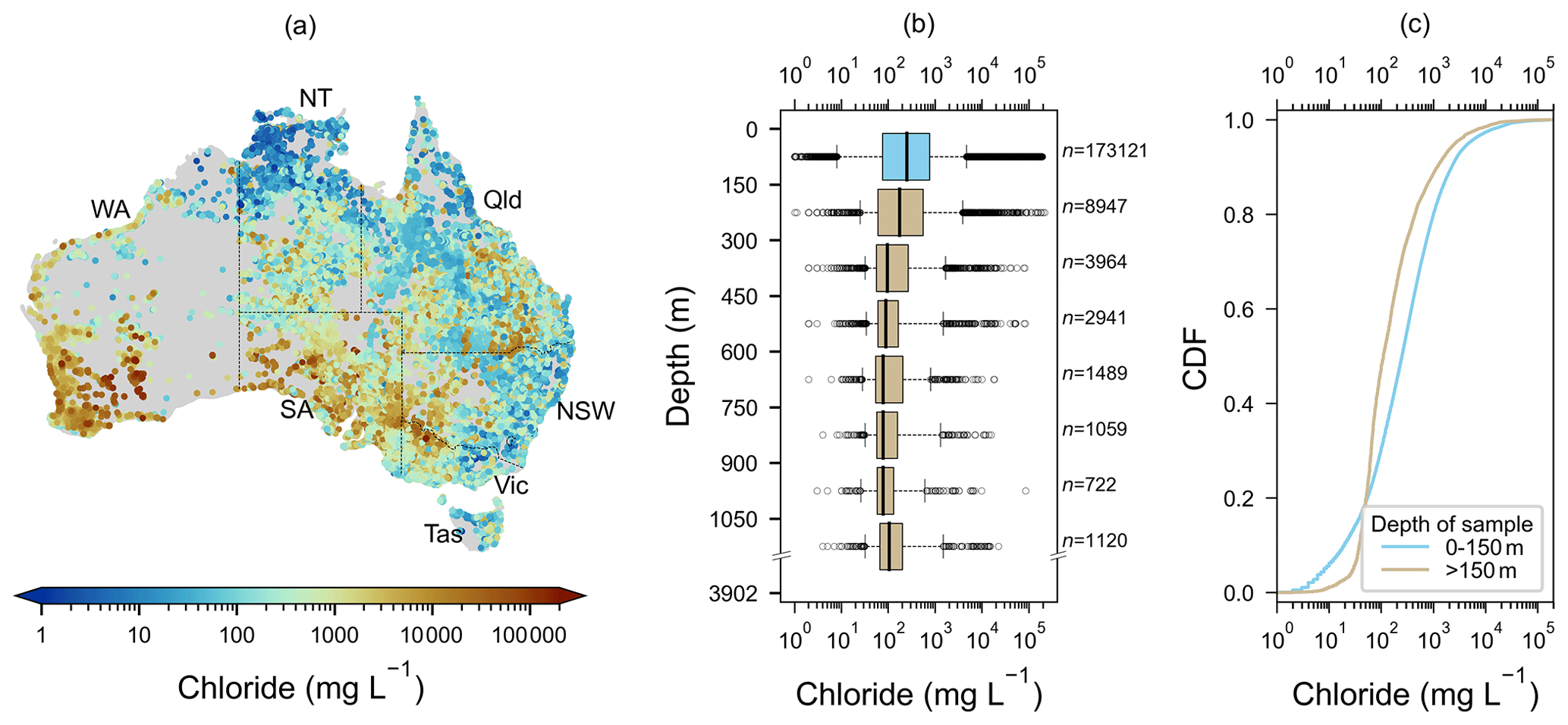
Figure 1 Spatial distribution of groundwater chloride (Cl_gw) shown as (a) locations and concentrations of Cl_gw with Australian states and territories marked as NT (Northern Territory), Qld (Queensland), NSW (New South Wales), Vic (Victoria), Tas (Tasmania), SA (South Australia) and WA (Western Australia); (b) box plots showing the depth distribution of Cl_gw. Box plots were binned by 150 m depth intervals except for the last box which contains Cl_gw measurements sampled from a depth of >1050 m. The blue box corresponds to the data used for recharge estimation. The upper and lower extents of the boxes represent the 75th and 25th percentiles of Cl_gw, respectively. The upper and lower whiskers represent the 95th and 5th percentiles of Cl_gw, respectively. The medians are shown as black lines and outliers are shown as hollow black circles. (c) The cumulative distribution function (CDF) of Cl_gw for shallow wells (depth of sample from 0 to 150 m) and deep wells (>150 m).

3 Results

3.1 Distribution of chloride measurements

The Cl_gw data collated in this study and their distributions are shown in Fig. 1. Cl_gw varies widely across the Australian continent, ranging from 1 to >200 000 mg L⁻¹ (Fig. 1a). Moderate to high Cl_gw concentrations predominantly occur in inland Australia. High Cl_gw concentrations are particularly prominent in southern Australia, in areas including the Murray–Darling Basin near the South Australia–Victoria–New South Wales junction where dryland salinity issues have been reported (e.g. Cartwright et al., 2007). Other Cl_gw hotspots such as in southern Western Australia correspond with where salt lakes exist (e.g. Bowen and Benison, 2009). As expected, the lowest Cl_gw concentrations are mainly located in the monsoon-influenced tropical north of Australia and along much of the temperate east coast of Australia, where rainfall is typically high (>1000 mm yr⁻¹; Fig. 1a).

Figure 1b shows the variation in chloride by depth. Most of the data are within 150 m of the ground surface (n=171 681; median Cl_gw is 250 mg L⁻¹). The median Cl_gw decreases with depth between 0 and 900 m, followed by an increase between 1050 and 3902 m. This notably contrasts with other regions in the world (e.g. Ferguson et al., 2023) due to Australia's unique climatic and geologic conditions (see Fig. S2 for more details).

The cumulative distribution function (CDF) plot (Fig. 1c) shows the difference in Cl_gw distribution between shallow (<150 m) and deep (>150 m) bores in Australia, with the shallow bores spanning a much wider range of Cl_gw values compared to the deeper bores. The CDF plot also highlights the proportionally lower number of low Cl_gw values (47 % of deep bores have Cl_gw<100 mg L⁻¹) and the lower median value of deeper bores (median Cl_gw is 110 mg L⁻¹) compared to shallow bores (30 % of shallow bores have Cl_gw<100 mg L⁻¹; median Cl_gw is 250 mg L⁻¹).

3.2 Recharge estimates and data filtering

Figure 2 shows the data filtering process applied to remove values that do not meet the assumptions required to apply the CMB method. It is important to note that the same bores that were excluded from R₅₀ during each step of the data filtering process (Fig. 2) were also excluded from R₅ and R₉₅. The recharge dataset prior to data filtering is provided as an electronic data file in the supporting information.

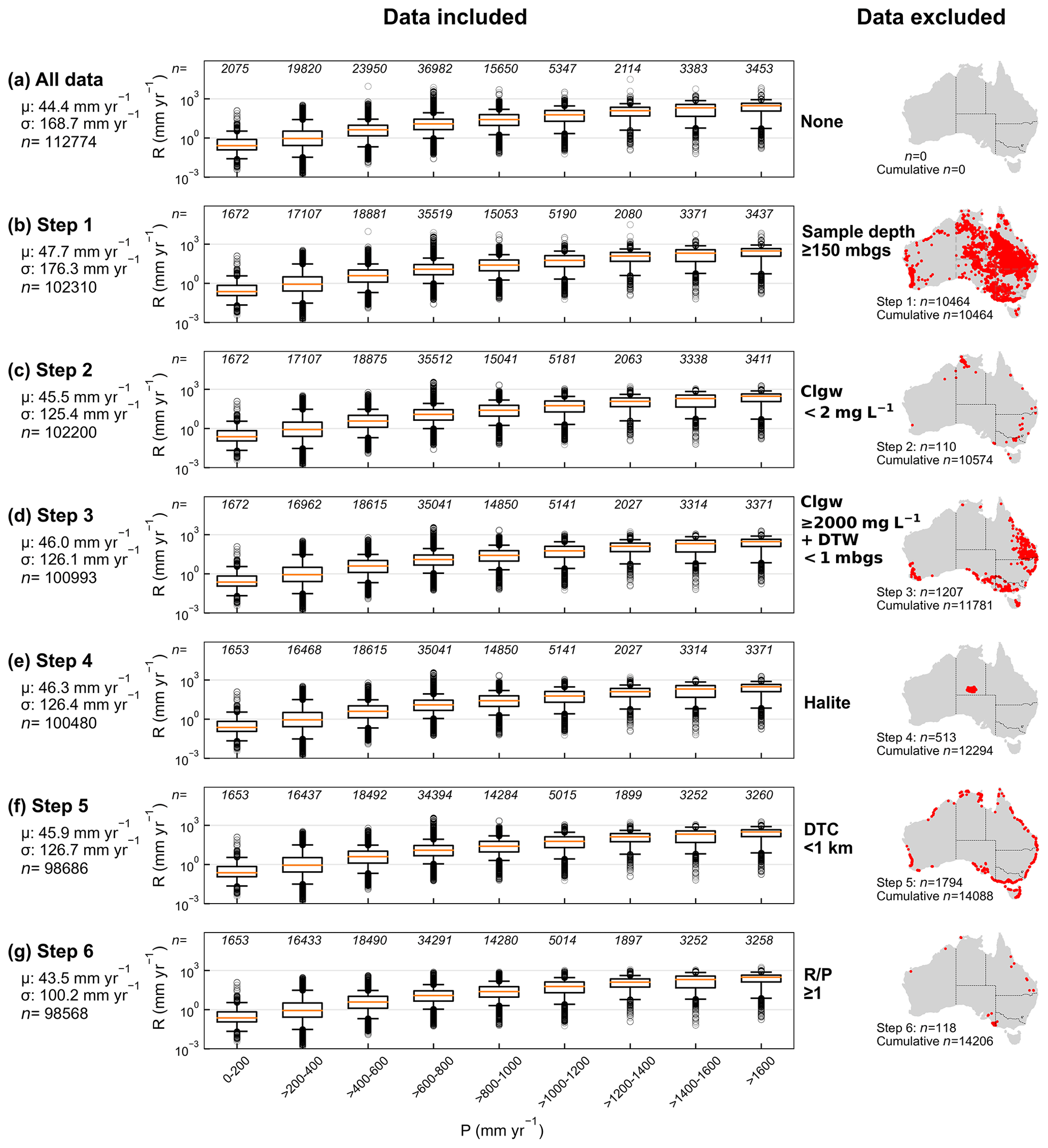
Figure 2 Data filtering process showing all data (a) and the groundwater recharge rate (R; mm yr⁻¹) estimates that were included at each step with statistics for R₅₀ (mean, standard deviation and number of measurements remaining) and box plots for R₅₀ binned by P at 200 mm yr⁻¹ intervals (except the >1600 mm yr⁻¹ bin). The upper and lower extents of the boxes represent the 75th and 25th percentiles of R₅₀, respectively. The upper and lower whiskers represent the 95th and 5th percentiles of R₅₀, respectively. The medians are shown as orange lines and outliers are shown as hollow black circles. The remaining number of measurements at each step is shown above the box plot. The maps on the right show the location of data, the number of measurements removed and cumulative number of measurements removed at each step.

The box plots in Fig. 2 present the R₅₀ distribution binned by P in 200 mm yr⁻¹ intervals (except the >1600 mm yr⁻¹ bin) at each step after data filtering. P ranged from 109 to 4231 mm yr⁻¹. The 600–800 mm yr⁻¹ bin contained the greatest number of R₅₀ values (∼33 %), followed by the 400–600 mm yr⁻¹ bin (∼21 %). Throughout the data filtering process, each bin was affected in different ways. R₅₀ values in the 400–600 mm yr⁻¹ bin had the highest number of exclusions (n=5460 between Fig. 2a and g). While the number of exclusions from the 0–200 mm yr⁻¹ bin was low (n=422), as a percentage this was a substantial cut of ∼20 % to the recharge estimates within this P range.

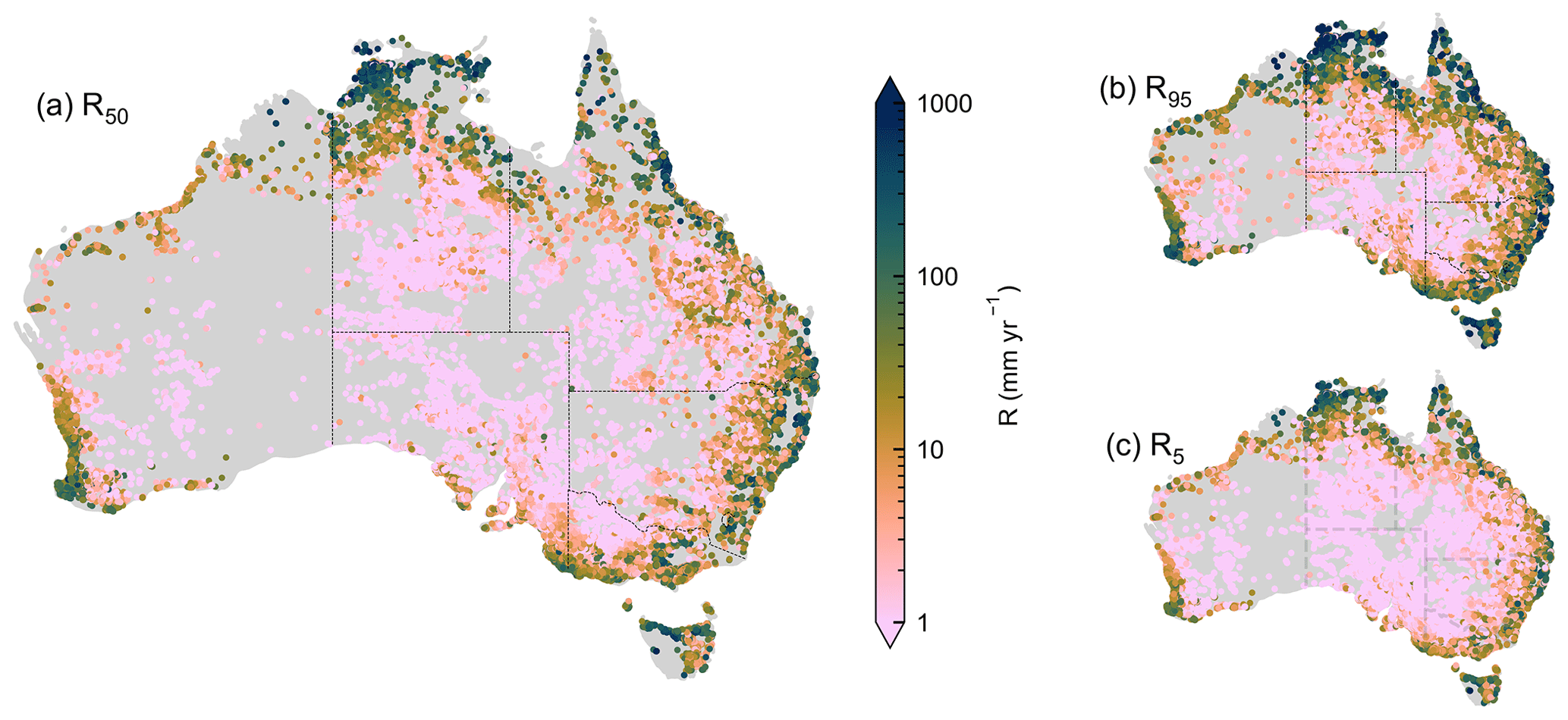
Figure 3 Groundwater recharge rates (R; mm yr⁻¹) estimated using CMB from 98 568 bores. Maps show (a) median recharge (R₅₀), (b) 95th-percentile recharge (R₉₅) and (c) 5th-percentile recharge (R₅) rates.

A map visualising the spatial locations of data being removed is shown for each step of the data filtering process in Fig. 2 (Fig. 2; right column). While clear spatial trends could be inferred from data removed in step 1 where deep bores were removed from the dataset (e.g. mostly bores in the Great Artesian Basin), step 4 where known halite deposits were removed (e.g. Amadeus Basin halite deposit) and step 5 where bores near the coast were removed, no obvious factors could be identified from most of the other steps without detailed analyses. A visual assessment shows that bores removed in step 3 broadly align with areas likely to contain areas of high hazard or risk of dryland salinity (National Land and Water Resources Audit, 2001).

At the end of the data filtering process (Fig. 2g) ∼12 % of the original dataset was removed, leaving 98 568 recharge values. Overall, the change in mean R₅₀ (μR₅₀) was minimal, with ∼2 % decrease from an initial μR₅₀ of 44.3 to 43.5 mm yr⁻¹. The largest change in μR₅₀ between steps was in the depth-filtering step (i.e. sample depth > 150 m b.g.s.), with a 7 % increase in μR₅₀ (Fig. 2b). Removing sample depths more than 150 m b.g.s. is crucial because most of the deep bores are located within the Great Artesian Basin and similar deep confined aquifers. The recharge area of these deep systems is likely to be hundreds of kilometres away from the bore location, whereas our analyses assume recharge occurs within the 0.05°×0.05° pixel from the chloride deposition map that contains the bore.

It is important to note that while the overall μR₅₀ did not change significantly at the end of the data filtering process, the standard deviation of R₅₀ (σR₅₀) decreased by ∼40 %. The noticeable decrease in σR₅₀ is the result of the exclusion of high recharge values generated from chloride concentrations < 2 mg L⁻¹ in step 2 (Fig. 2c) and the exclusion of recharge values with $R/P>\mathrm{1}$ in step 6 (Fig. 2g). While step 6 (Fig. 2g) did not remove a significant number of R₅₀ values (n=118), it is likely that many R₅₀ values with $R/P>\mathrm{1}$ had already been removed in previous steps of the data filtering process due to other factors.

The resulting recharge estimates for R₅₀, R₉₅ and R₅ are shown in Fig. 3a–c, respectively. The mean values of recharge rates for R₅₀, R₉₅ and R₅ are 43.5, 113.4 and 25.8 mm yr⁻¹, respectively.

As expected, high recharge rates are mostly located in areas with high precipitation, i.e. in the tropical north, along the east coast and in north-western Tasmania (see Fig. 3 and rainfall map in Fig. S1a), while low recharge rates are mostly located inland from the coast. However, there is variability in recharge rates, spanning 1–3 orders of magnitude in inland areas, that cannot be explained by rainfall variability alone.

The majority of R₅₀ values in our dataset are either low or moderate: 1–10 mm yr⁻¹ (35 %) or 10–100 mm yr⁻¹ (38 %), respectively. Extremely low R₅₀ values (i.e. <1 mm yr⁻¹) constitute 16 % of the dataset, while high R₅₀ values (i.e. 100–1000 mm yr⁻¹) constitute 11 % of the dataset. Only 0.01 % of R₅₀ values are extremely high (i.e. >1000 mm yr⁻¹). The point datasets of R₅₀, R₅ and R₉₅ before and after the data filtering process are available as electronic data files in the supporting information.

3.3 Random forest models and feature importance

To explore the effects of the selection of variables on the random forest analyses (Table 1), different variable groupings were investigated as input features to train different R₅₀ random forest models. Table 2 outlines combinations of variables and their impact on various fit metrics, showing the highest R² values, the lowest root mean square error (RMSE), the mean absolute error (MAE) and the number of trees used.

Table 2 Best results from random forest R₅₀ models developed using different variable groupings, showing the optimal number of trees in each forest, training score (R²), external validation test score (R²), root mean square error (RMSE) and mean absolute error (MAE). P is precipitation, AI is aridity index, PET is potential evapotranspiration, KG is Köppen–Geiger zone, RS is rainfall seasonality, DTC is distance to coast, RD is regolith depth, WTD is water table depth, SP is slope percentage, E is elevation, G is geology, SC is soil class, CP is clay percentage, SiP is silt percentage, SaP is sand percentage, NDVI is the normalised difference vegetation index and VC is vegetation category. ^* Denotes the model selected for further analyses.

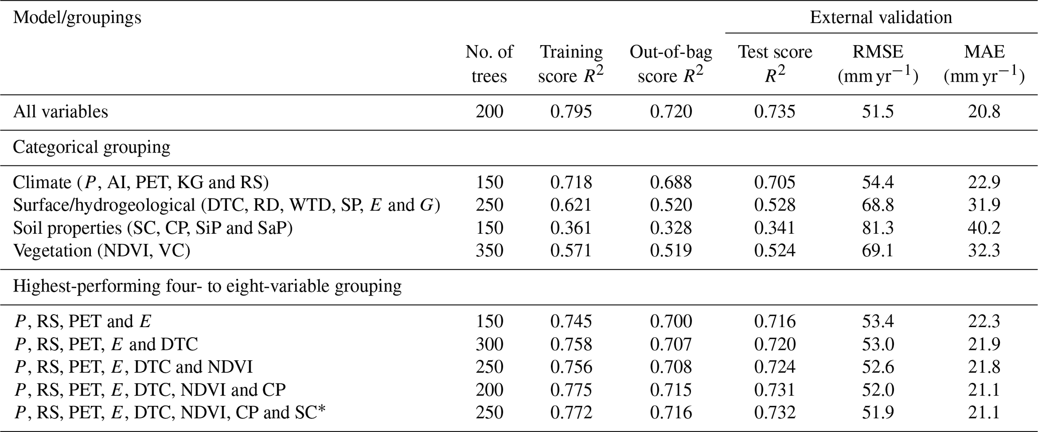
The results in Table 2 have also been influenced by the selection of optimal hyperparameters, such as the number of trees, maximum depth of trees and maximum features. Aside from grouping variables categorically by climate, surface/hydrogeology, soil properties and vegetation, various other groupings ranging from four to eight variables were also explored. Exploring fewer input variables allows us to assess whether a model trained on fewer variables could achieve similar model accuracy while being less computationally expensive. The strongest-performing four- to eight-variable groups are shown in Table 2. The best-performing eight-variable model trained with 250 trees achieved a training score R² of 0.772, an external validation test score R² of 0.732, RMSE of 51.9 mm yr⁻¹ and MAE of 21.1 mm yr⁻¹, which are similar to the all-variable model (Table 2). Model accuracy does not improve when a ninth variable (either regolith depth, water table depth, geology, sand percentage, slope percentage, vegetation class, Köppen–Geiger zone, aridity index or silt percentage) was added (see Table S2); hence, the best-performing eight-variable model was chosen.

Table 2 demonstrates the importance of the climatological variables, for example, which produced an external validation test score R² value of 0.705, similar to the maximum external validation test score obtained across all parameter combinations (0.735). The R₅₀ random forest model selected for further analyses (the best-performing eight-variable model) consists of the variables precipitation (P), rainfall seasonality (RS), potential evapotranspiration (PET), elevation (E), distance to coast (DTC), normalised difference vegetation index (NDVI), clay percentage (CP) and soil class (SC) (Table 2, bottom row). This observation highlights that while the climatological variables are strong controls on recharge, other variables related to surface processes, hydrogeology, soil properties and vegetation are also important. The vegetation model (containing the variables NDVI and vegetation class), which had the second-highest score in the categorical groupings, suggests that in Australia vegetation could be a more important control on recharge than surface/hydrogeological and soil property variables.

Out of the eight input variables used in our best-performing R₅₀ random forest model, P, RS, PET and NDVI are ranked highest, as shown in the feature importance plot in Fig. 4. The feature importance plots for the R₅ and R₉₅ random forest models are provided in Figs. S4 and S5, respectively. For comparison, the feature importance plot for the R₅₀ all-variable model is provided in Fig. S6.

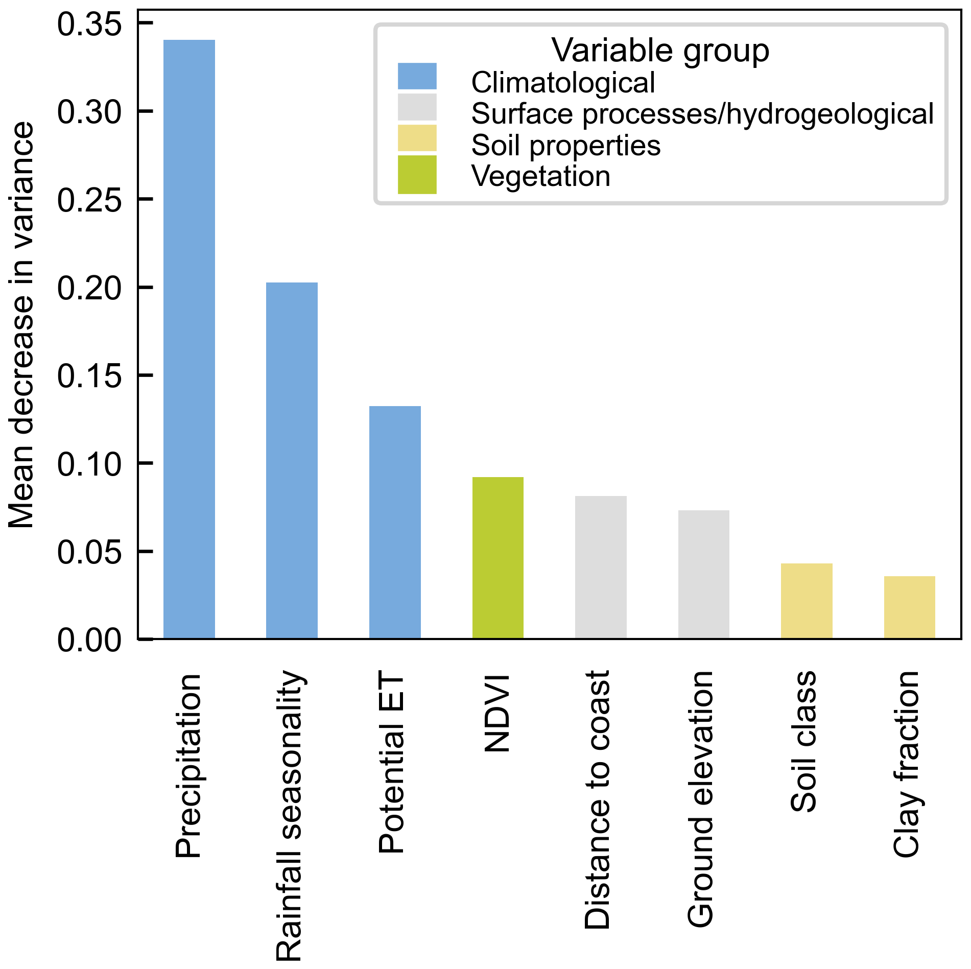
Figure 4 Mean feature importance through mean decrease in variance for the R₅₀ best-performing eight-variable model (250 trees). The features are grouped according to the climatological, surface process/hydrogeological, soil property and vegetation variable groups depicted in Table 1.

The R₅₀ random forest model achieved a training score of R²=0.772, an “out-of-bag” score of R²=0.716, an external validation test score of R²=0.732 and a 10-fold cross-validation R²=0.715, with 250 trees in the random forest (Fig. 5). The relatively small difference between the training score and external validation test score indicates that our model is not over-fitting the training data. The similar R² values across different model evaluation methods indicate that our model should perform relatively well with unseen data. Figure 5a shows that our model tends to overestimate lower recharge values and underestimate higher values.

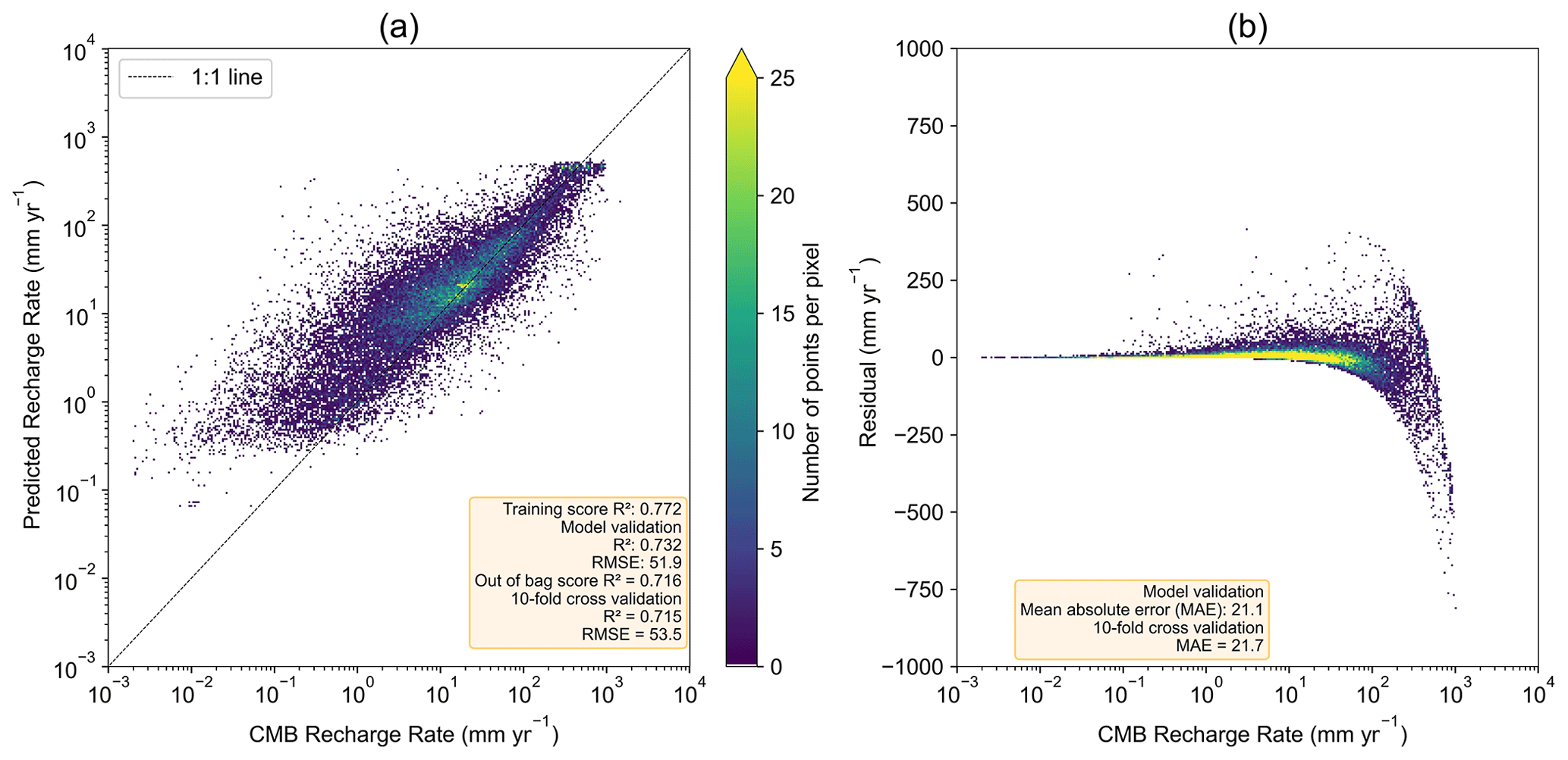
Figure 5 Model validation results for the selected R₅₀ model trained using 250 trees, showing (a) CMB recharge rate (R₅₀) versus predicted recharge rate (showing the 1:1 line) and point density and (b) CMB recharge rate (R₅₀) versus residuals (predicted recharge rate minus CMB recharge rate) and point density.

Figure 5b further demonstrates this point. For example, for CMB recharge values between 0.001 and 30 mm yr⁻¹, our model tends to overestimate recharge, while at moderate to higher recharge rates (i.e. >30 mm yr⁻¹) our model tends to underestimate recharge. At high to extremely high recharge rates (i.e. >470 mm yr⁻¹) our model only produces underestimates, which could be the result of underrepresentation of samples in extremely high recharge areas. The residuals at the higher end of recharge in Fig. 5b may appear seemingly large, but the majority of them represent errors of less than 40 %.

Compared to the μR₅₀ of 43.5 mm yr⁻¹ in Fig. 2g, the RMSE of 51.9 mm yr⁻¹ from external validation of our model (Fig. 5a) might suggest relatively high variability in and overall inaccuracy of model predictions. However, Fig. 5a shows that most of the recharge rate estimates lie near the 1:1 line (as shown by the density of pixels in the colour map). When assessing only R₅₀<1 mm yr⁻¹ for the validation results (Fig. 5), we obtain an RMSE of 12.4 mm yr⁻¹ or >1000 %; however, percentage errors can be misleading when assessing errors in low values. This is similarly the case for R₅₀ from 1 to 10 mm yr⁻¹ (RMSE= 19.4 mm yr⁻¹), 10–100 mm yr⁻¹ (RMSE= 29.8 mm yr⁻¹) and 100–1000 mm yr⁻¹ (RMSE= 140.7 mm yr⁻¹). Evaluating errors in different recharge ranges reveals that some errors are not as severe as they may appear. Model validation results for the R₅ and R₉₅ recharge models are provided in Fig. S7.

The random-forest-generated groundwater recharge rate (R₅, R₅₀ R₉₅) maps of Australia (utilising P, RS, PET, E, DTC, NDVI, CP and SC) are shown in Fig. 6a–c.

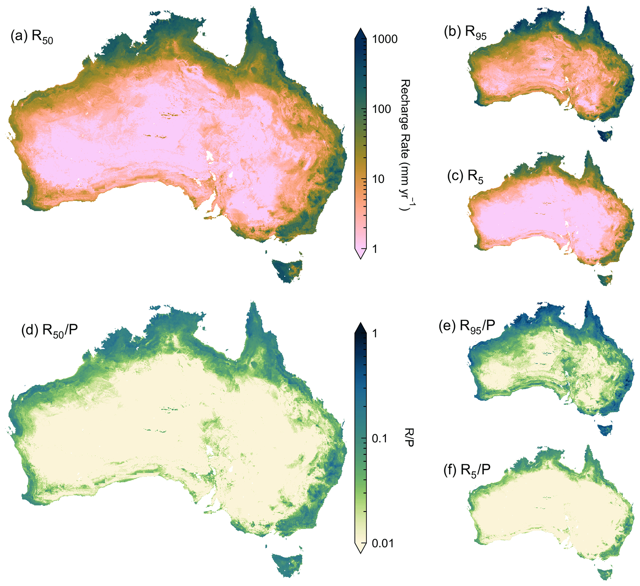
Figure 6 Gridded groundwater recharge rate map of Australia generated using the highest-performing random forest model, shown as (a) median recharge rate (R₅₀), (b) 95th-percentile recharge rate (R₉₅) and (c) 5th-percentile recharge rate (R₅) values. Gridded recharge ratio ($R/P$) map of Australia, shown as (d) $R_{\mathrm{50}}/P$, (e) $R_{\mathrm{95}}/P$ and (f) $R_{\mathrm{5}}/P$. Gridded datasets are available for download; see “Code and data availability ” section.

The CMB method provides recharge estimates that span the residence time of the groundwater (Crosbie et al., 2010a); hence, the recharge outputs produced in Fig. 6 represent recharge that has occurred over the longer term (e.g. hundreds to thousands of years). The variability in modelled recharge is highest within the arid Köppen–Geiger zones, which cover almost 80 % of the Australian continent, with R₅₀ ranging between ∼0.03 and 278 mm yr⁻¹ and a mean of 6.3 mm yr⁻¹ (n pixels = 220 947). In the temperate Köppen–Geiger zones, which cover almost 12 % of the Australian continent, R₅₀ ranges between ∼0.6 and 522 mm yr⁻¹, with a mean of ∼60 mm yr⁻¹ (n pixels = 33 177). In the tropical climates, which only cover 8 % of the Australian continent, R₅₀ ranges between ∼2.6 and 621 mm yr⁻¹, with a mean of ∼125 mm yr⁻¹ (n pixels = 22 897). As shown in Fig. 6b and c, uncertainties in recharge estimates can vary by orders of magnitude, regardless of climate zone. For example, the town of Tully, Queensland (located in the Af tropical Köppen–Geiger zone at lat −17.934°, long 145.925°), has the highest average rainfall in Australia (>3100 mm yr⁻¹) and the highest modelled R₅₀, ∼621 mm yr⁻¹. However, the uncertainty ranges from 393 to 1759 mm yr⁻¹. The town of Coober Pedy, South Australia (located in the BWh arid Köppen-Geiger zone at lat −29.012°, long 134.753°), has one of the lowest average rainfalls in Australia (<150 mm yr⁻¹) and a modelled R₅₀ of ∼0.38 mm yr⁻¹, with uncertainty ranging from 0.09 to 0.56 mm yr⁻¹.

The proportion of rainfall that becomes recharge, represented by the recharge ratios ($R_{\mathrm{5}}/P$, $R_{\mathrm{50}}/P$ and $R_{\mathrm{95}}/P$), is shown as gridded maps in Fig. 6d–f, respectively. Like recharge, the variability in modelled $R_{\mathrm{50}}/P$ is the highest in the arid Köppen–Geiger zones, ranging over 4 orders of magnitude, from ∼0.0001 to 0.42 (mean= 0.02, n pixels = 220 947). In temperate and tropical climates, $R_{\mathrm{50}}/P$ ranges are smaller, from ∼0.002 to 0.36 (mean= 0.06, n pixels = 33 177) and ∼0.003 to 0.35 (mean= 0.11, n pixels = 22 897), respectively. The ranges in $R/P$ reduce significantly when assessing the 5th and 95th percentiles (i.e. 90 % of the values are in the following ranges for arid, temperate and tropical zones: ∼0.002–0.06, ∼0.01–0.15 and ∼0.03–0.20, respectively). It should be noted that some values of $R_{\mathrm{95}}/P$ exceed 1 due to the data filtering process only focusing on removing bores with $R/P>\mathrm{1}$ from the R₅₀ point recharge dataset. Therefore, both the R₉₅ gridded recharge dataset and point recharge dataset will contain some unrepresentative recharge values with $R/P$ values of more than 1. However, the number of values equates to <0.01 % of pixels in the $R_{\mathrm{95}}/P$ gridded map.

Box plots showing the distribution of modelled recharge values (R₅₀, R₅ and R₉₅) and modelled recharge ratios ($R_{\mathrm{5}}/P$, $R_{\mathrm{50}}/P$ and $R_{\mathrm{95}}/P$) categorised by arid, temperate and tropical Köppen–Geiger zones are shown in Fig. S8. The gridded maps of R₅₀, R₅ and R₉₅ are available as electronic text files in the supporting information.

4 Discussion

4.1 Groundwater recharge rate predictors

Clearly, precipitation has a strong control on groundwater recharge rates. While some studies have found long-term average precipitation to be the key predictor of recharge (e.g. MacDonald et al., 2021, and West et al., 2023), others have found other precipitation-related factors such as aridity index (e.g. Berghuijs et al., 2022) or seasonal rainfall (e.g. Fu et al., 2019) to be the most important. Some investigations highlighted the strong explanatory power of vegetation and soils in addition to climate-related variables (e.g. Petheram et al., 2002; Crosbie et al., 2010a; Mohan et al., 2018; and Moeck et al., 2020). Our R₅₀ random forest model incorporated eight variables from the climatological, surface process/hydrogeological, soil property and vegetation categories. Using these eight variables in the feature importance analyses, our study revealed that the four most important variables influencing recharge in Australia were precipitation (P), rainfall seasonality (RS), potential evapotranspiration (PET) and NDVI (Fig. 4). These four variables highlight the importance of climatic factors for the prediction of recharge, which agrees with other studies (e.g. Mohan et al., 2018; Berghuijs et al., 2022; West et al., 2023; and Huang et al., 2023). Overall, the ranking of variables highlighted in our study is most aligned with the ranking of predictors in Mohan et al. (2018), who found precipitation, PET and land use (vegetation) to be the top three factors controlling recharge globally.

The aforementioned studies cover vastly different spatial scales, ranging from regional areas (e.g. Fu et al., 2019, and Huang et al., 2023), the African continent (e.g. MacDonald et al., 2021, and West et al., 2023) and the Australian continent (e.g. Petheram et al., 2002, and Crosbie et al., 2010a) to all continents (e.g. Mohan et al., 2018; Moeck et al., 2020; and Berghuijs et al., 2022) and contain datasets with varying spatial distributions and resolutions. The spatial variability across these previous studies suggests that some studies can have a climatic bias depending on the climates included in the study area. For example, the chloride data used in our study to produce recharge estimates were mainly biased towards temperate and arid Köppen–Geiger zones (comprising ∼50 % and ∼40 % of the recharge dataset, respectively) and less so towards tropical zones (∼10 % of recharge values). The similarities and differences in climate types and recharge estimation techniques may influence the ultimate ranking of important variables and may be the reason for differences between studies.

It is important to highlight that while feature importance analyses can provide insight into important variables, overinterpretation should be avoided. The ranking of features in the feature importance plot can be affected by the choice of hyperparameters such as maximum features (e.g. limiting maximum features to a subset will avoid over-selection of the most important feature, such as precipitation in our case, during training of the random forest model). Feature importance may be influenced by factors such as variable cardinality (i.e. the tendency to give higher importance to variables with many unique levels, as they offer more opportunities for splitting the data; Strobl et al., 2007). Low cardinality of categorical features such as Köppen–Geiger zone, geology, soil class and vegetation class could be the reason for their relatively lower feature importance, as shown in Fig. S6. Variables with lower importance can compete with more important variables such that having more input variables does not necessarily improve performance of the model. Correlated variables can also outcompete each other, leading to unreliable feature importance rankings (Toloşi and Lengauer, 2011). Some highly correlated variable pairs likely act as proxies for each other during the training process when the subset of features randomly selected only contains one of the variable pairs. Such is likely the reason for the climate group being the most important in the all-variable model (Fig. S6). Similarly, the relationship between precipitation, distance to coast and elevation could explain why these variables also rank highly.

4.2 Comparison of groundwater recharge rate estimates with previous studies

The average groundwater recharge rate estimates produced for the Australian continent differ from those found in other studies for both point recharge (Fig. 3) and modelled recharge (Fig. 6). For example, the mean point recharge rate for the Australian studies collated by Crosbie et al. (2010a) was 257.2 mm yr⁻¹ (n=4360), compared to 43.5 mm yr⁻¹ in our study (n=98 568). Similar mean recharge values of 246.5 mm yr⁻¹ from Australian studies collated by Moeck et al. (2020; n=4579) and 244 mm yr⁻¹ from Berghuijs et al. (2022) were not surprising given that the data from Crosbie et al. (2010a) were used in both studies. The mean recharge rate for the Australian studies collated by Mohan et al. (2018) was much closer to our study, at 46.2 mm yr⁻¹. This is likely due to the much smaller dataset of Mohan et al. (2018; n=217) and limited spatial coverage – especially in tropical Northern Australia – compared to other studies.

The higher mean recharge values of the point data reported in other studies that cover Australia (e.g. Crosbie et al., 2010a; Moeck et al., 2020; and Berghuijs et al., 2022) compared to ours can be attributed to the difference in spatial distribution of recharge point estimates and the different recharge estimation methods used. Several differences in the methods are important, including the following differences.

1. A total of 60 % of the estimates in Crosbie et al. (2010a) and Moeck et al. (2020) were from an earlier study (Crosbie et al., 2009), which used a simpler CMB method and an older chloride deposition map to calculate recharge (see chloride deposition maps in Fig. S9b).

2. Our method incorporates the most recent improved chloride deposition map with enhanced data and spatial coverage (Wilkins et al., 2022).

3. There are key differences in chloride deposition rates between the different chloride deposition maps, especially within 50 km of the coastline, that can significantly affect the resulting recharge rate (see chloride deposition maps in Fig. S9).

4. The mean of the 2722 CMB recharge estimates from Crosbie et al. (2009) is 388 mm yr⁻¹. Excluding the 2722 CMB estimates from Crosbie et al. (2009), the mean of the remaining 1620 estimates from Crosbie et al. (2010) that were estimated from 14 different methods (including 38 % from CMB, 25 % from transient soil CMB and 9 % from water table fluctuation) is 40 mm yr⁻¹. The estimates from Crosbie et al. (2009) are likely overestimates and were flagged by Crosbie et al. (2010a) as having very little quality control.

5. Our approach accounts for chloride lost to runoff in the estimation of recharge, resulting in a reduction in our recharge rates compared to the simpler method used in Crosbie et al. (2009), which does not consider this factor.

6. Following the approach used by Crosbie et al. (2018) and Crosbie and Rachakonda (2021), our methodology is stochastic, performing 1000 recharge calculations to generate a probability distribution. We present the median and an error range taken as the 5th and 95th percentiles of the distribution to provide a more robust interpretation of the results.

The spatial distribution of the recharge estimates (in our study relative to previous investigations) is important because the climate at the location of the recharge estimate strongly influences the annual recharge rate (Moeck et al., 2020). Figure 7 demonstrates this point using Australian climate zones that are classified according to different aridity index values, i.e. in order of increasing aridity or decreasing recharge potential (humid, dry subhumid, semi-arid, arid and hyper-arid; based on United Nations Environment Programme, 1997).

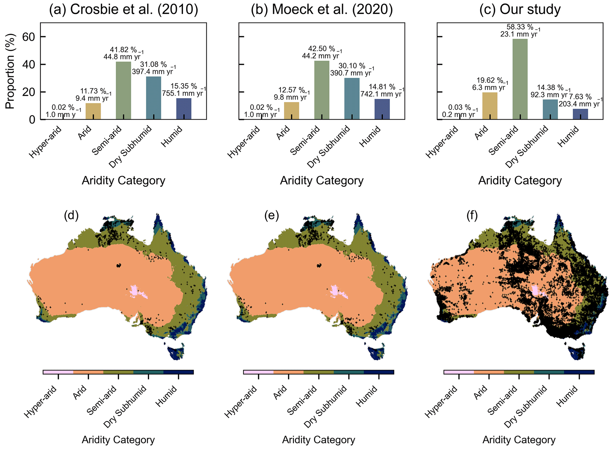
Figure 7 Histograms and maps showing the difference in spatial distribution and proportion (%) of the point recharge dataset of (a, d) Crosbie et al. (2010a), (b, e) Moeck et al. (2020) and (c, f) our study, which are located in various aridity classes (hyper-arid, arid, semi-arid, dry subhumid and humid; United Nations Environment Programme, 1997). The proportion (%) and mean recharge (mm yr⁻¹) are shown in the histograms above each bar.

The proportion of recharge estimates from Crosbie et al. (2010a) and Moeck et al. (2020) located in dry subhumid and humid aridity classes is significantly higher than in our dataset (Fig. 7), with 46.43 % and 44.91 % for Crosbie et al. (2010a) and Moeck et al. (2020), respectively, compared to 22.01 % in our study. The mean recharge rates in Crosbie et al. (2010a) and Moeck et al. (2020) for each aridity category are all higher than in our study – particularly the dry subhumid and humid categories, which are 3–4 times higher. The higher proportion of estimates in the dry subhumid and humid climate zones, together with the significantly higher mean recharge rates in these climates, results in a higher overall mean recharge rate for the Crosbie et al. (2010a) and Moeck et al. (2020) datasets compared to our study. Further details including limitations in the comparisons with Crosbie et al. (2010a) and Moeck et al. (2020) are provided in the supporting information.

Studies that collated recharge estimates from other continents have also reported higher recharge rates than our point estimates. For example, MacDonald et al. (2021) reported median decadal point recharge estimates from compiled studies for different aridity zones on the African continent, with arid, semi-arid and humid areas equivalent to 6, 20 and 130 mm yr⁻¹, respectively. Point estimates of recharge from our study had median values of 1.1, 8.0 and 45.8 mm yr⁻¹ for arid, semi-arid and humid areas in Australia, respectively, across these climate zones. This suggests that in the long term, aquifer systems in Australia are replenished on average at a rate 2–4 times lower than those in Africa.

Regarding the methods used, the CMB method produces long-term average diffuse groundwater recharge rates that are lower compared to other methods, including the water table fluctuation method that estimates modern recharge. For example, methods such as the water table fluctuation method and tritium method tend to estimate different recharge rates relative to those obtained via the CMB method, particularly in Australia where modern recharge rates have increased due to large-scale land clearing (Cartwright et al., 2007). Measurements using the water table fluctuation method will also be heavily influenced by focused recharge in areas where indirect recharge processes are dominant (e.g. leakage from ephemeral streams in arid regions; Cuthbert et al., 2016), as opposed to the diffuse recharge measured by the CMB method. These observations likely highlight the importance of considering recharge estimation type in the collation and use of large datasets. For example, recharge studies comparing recharge estimation techniques have found large differences across different methods (e.g. Cartwright et al., 2007, 2020; King et al., 2017; and Walker et al., 2019).

The mean modelled (R₅₀) recharge rate from our gridded recharge rate map was 22.7 mm yr⁻¹, which is significantly lower than modelled global estimates. For example, Mohan et al. (2018) reported a long-term global average recharge of 134 mm yr⁻¹, whereas Müller Schmied et al. (2021) reported a global mean diffuse recharge rate of 111 mm yr⁻¹. The significant difference between these modelled recharge values is likely due to the large proportion of arid and semi-arid areas in Australia. Our gridded map contains 278 253 pixels, ∼80 % of which are in an arid Köppen–Geiger climate (see Fig. S11), compared to ∼26 % of the global land area that is classified as arid (Gaur and Squires, 2018). The mean modelled recharge for the Australian continent was not reported in either Mohan et al. (2018) or Berghuijs et al. (2022). However, Berghuijs et al. (2022) highlight that their recharge estimates are higher than those presented in other global studies (e.g. Döll and Fiedler, 2008; de Graaf et al., 2015; Mohan et al., 2018; and Müller Schmied et al., 2021) and are therefore, on average, likely to be higher than those presented here. We highlight that numerical outputs from these studies should be provided more routinely. Sharing these numerical outputs could facilitate further comparisons and produce more useful outputs for potential users.

4.3 Limitations and implications

In this study, the assumptions for estimating recharge using the CMB method were implemented through a data filtering process (Sect. 2.4), which was crucial to improving the reliability of inputs into our model. While we assume that erroneous recharge estimates have been removed during the data filtering process, some criteria that were assessed in other studies (e.g. Crosbie et al., 2022, and Crosbie and Rachakonda, 2021) were not considered here due to the challenges of implementing them on a continental scale. For example, excluding measurements from bores screened within alluvium (e.g. Crosbie et al., 2022) would require a thorough understanding of local conceptual models and hydrogeological processes (e.g. cross-aquifer interaction) and existing recharge processes (e.g. flooding). By not excluding bores located in alluvium, point and modelled recharge estimates for these bores can be underestimated if additional chloride not sourced directly from rainfall is present, for example, through the application of irrigation water or chloride-based fertilisers (e.g. potassium chloride).

The tendency of our model to underestimate recharge where moderate to higher recharge rates (i.e. 30–1000 mm yr⁻¹) were estimated from the CMB method may be related to a skew in the distribution of our point recharge dataset towards lower recharge rates. The tendency toward overestimation could be due to the aggregation of random forest leaf node values and tree predictions using the arithmetic mean, which can be biased by large outlier values.

Large areas (e.g. inland Western Australia) had no chloride data, and hence, the modelled recharge for these areas can be subject to larger ranges of uncertainty. No geological dataset is available that provides detailed spatial information on the permeability of bedrock; therefore, modelled recharge rates can be significantly overestimated in areas such as where low-permeability bedrock crops out at the surface and underestimated in areas where highly fractured bedrock exists. Similarly, we highlight that users should be aware of the range of uncertainty in the modelled recharge when using values from the analyses presented here. The same message was emphasised by Leaney et al. (2011) and Crosbie et al. (2010a) for the “method of last resort”. As is the case with all hydrogeological measurements and models, users of our modelled recharge rates should exercise expert judgement and determine whether the estimates are reliable and fit for purpose. Preference should always be given to the collection of field data to constrain recharge estimates where possible.

Our study provides an extensive database of groundwater chloride measurements and rigorously interpreted groundwater recharge rate estimates at a high spatial resolution that holds potential for further use for researchers and water resource managers. We present a more robust stochastic recharge rate estimator modified from CMBEAR (Irvine and Cartwright, 2022) to include the runoff coefficient term utilised in recent regional Australian studies (e.g. Crosbie et al., 2018, and Crosbie and Rachakonda, 2021). Our study produced long-term recharge maps of the Australian continent. While Australian recharge maps have been produced previously (e.g. Leaney et al., 2011), this is the first time that a model of such scale has been developed from recharge estimates derived from only a single recharge estimation technique. Furthermore, by providing the Python code, point estimates and gridded map, we facilitate a transparent and reproducible workflow that enables the broader community to utilise our methodology or further improve the approach.

5 Conclusions

We produce a groundwater recharge rate dataset for Australia with a high resolution based on an improved chloride mass balance (CMB). This combines more than 200 000 compiled chloride measurements, existing chloride deposition maps, 17 national spatial gridded datasets and a rigorous groundwater recharge rate estimation workflow. We enhance an open-source Python tool, CMBEAR, and leverage existing methodologies (e.g. Crosbie et al., 2018) to provide an efficient, reproducible and transparent stochastic approach that can be applied to anywhere in Australia. This approach quantifies uncertainty by creating groundwater recharge rate probability distributions, providing the 5th and 95th percentiles of point groundwater recharge rate estimates (R₅ and R₉₅) using distributions of groundwater chloride, runoff and chloride deposition.

We utilise subsets of the CMB recharge datasets (R₅, R₅₀ and R₉₅) to train and test three random forest regression models for the purposes of upscaling point recharge estimates and assessing the relative importance of recharge predictors. We show that climate-related variables (i.e. precipitation, rainfall seasonality and PET) have the strongest control on the groundwater recharge rate, but vegetation (NDVI) is also important. Other geographic and soil property variables ranked lower but are still relatively important. The importance of climate and vegetation as recharge predictors is generally aligned with global recharge studies. The use of only 8 of the 17 variables demonstrates that similar prediction performance can be achieved with fewer variables, while reducing computation time and ensuring adequate performance on unseen data.

We present a gridded map of groundwater recharge rate estimates and uncertainties that could be valuable where data required to estimate groundwater recharge rates may be scarce or not available. Our groundwater recharge model utilises a data-driven approach based on a single recharge estimation technique to provide long-term groundwater recharge rates. Our CMB-based groundwater recharge rates are considerably lower than other studies including global water balance models (e.g. Döll and Fiedler, 2008; de Graaf et al., 2015; and Müller Schmied et al., 2021). This is likely due to the fact that CMB operates at longer timescales that span the residence time of the groundwater (e.g. chloride can take between 4000 and 40 000 years to accumulate in the Murray Basin, South Australia; Scanlon et al., 2006). Contrary to this, global water balance models estimate modern recharge (i.e. over the last century, where climate and soil data are available). Recharge estimation methods operating over modern timescales tend to be impacted by land-use change. For example, Scanlon et al. (2006) demonstrate groundwater recharge both pre- and post-clearing in an Australian context, showing a significant change (increase) in recharge. We emphasise that the appropriate recharge timescales (e.g. long-term or modern) and mechanisms (e.g. diffuse or focused recharge) should be taken into consideration when collating recharge values produced from different techniques for the purpose of modelling recharge. We recommend that users exercise care and expert judgement when utilising the groundwater recharge rate estimates from these large-scale groundwater recharge models.

By applying an improved version of the most widely used recharge estimation method (e.g. Moeck et al., 2020, and Crosbie et al., 2010b), we provide a robust approach to automate the estimation of long-term diffuse groundwater recharge rates, including uncertainties. With chloride data being amongst the most common of groundwater analytes, there are significant opportunities to conduct similar analyses elsewhere.