Influence of bank slope on sinuosity-driven hyporheic exchange flow and residence time distribution during a dynamic flood event

This study uses a reduced-order two-dimensional (2-D) horizontal model to investigate the influence of the riverbank slope on the sinuosity-driven hyporheic exchange process along sloping alluvial riverbanks during a transient flood event. The deformed geometry method (DGM) is applied to quantify the displacement of the sediment–water interface (SWI) along the sloping riverbank during river stage fluctuation. This new modeling approach serves as the initial step focusing on the impact of the bank slope on the hyporheic exchange flux (HEF) and the residence time distribution (RTD) of pore water in the fluvial aquifer for a sinuosity-driven river corridor. Several controlling factors, including sinuosity, alluvial valley slope, river flow advective forcing and duration of flow, are incorporated into the model to investigate the effects of bank slope on aquifers of variable hydraulic transmissivity. Compared to simulations of a vertical riverbank, sloping riverbanks were found to increase the HEF. For sloping riverbanks, the hyporheic zone (HZ) encompasses a larger area and penetrated deeper into the alluvial aquifer, especially in aquifers with smaller transmissivity (i.e., due to increased hydraulic conductivity or reduced specific yield). Furthermore, consideration of sloping banks as compared to a vertical riverbank can lead to both underestimation and overestimation of the pore water travel time. The impact of bank slope on residence time was more pronounced during a flood event for high-transmissivity aquifer conditions, while it had a long-lasting influence after the flood event in lower-transmissivity aquifers. Consequently, the impact of bank slope decreases the travel time of water discharging into the river relative to base flow conditions. These findings highlight the need for (re)consideration of the importance of complex riverbank morphology conceptualization in numerical models when accounting for the HEF and RTD. The results have potential implications for river management and restoration and the management of river and groundwater pollution.

1 Introduction

The hyporheic zone (HZ) can be described as the region that connects the river channel and adjacent aquifer and includes the riverbed and riverbanks. Mixing and transport of different water types (groundwater, surface water) and water ages in the HZ driven by hydrodynamic and hydrostatic factors cause spatially and temporally varying exchange of water and biogeochemical species between the river channel, riverbed and aquifer (Cardenas, 2009b; Hester and Gooseff, 2010; Krause et al., 2011, 2017, 2022; McClain et al., 2003; Boano et al., 2014). The hyporheic exchange flux (HEF) represents the interaction flux between surface water and groundwater in vertical (e.g., bedform-driven) and horizontal/lateral (e.g., meander-driven) directions, which can add to general regional groundwater exfiltration and infiltration. The distribution of hyporheic flow paths strongly determines the spatial and temporal distribution of hydrogeochemical characteristics of water within the riverbed and the wider river corridor, as well as the formation of so-called hot zones and hot moments (Krause et al., 2013, 2017; Cardenas, 2015; Pinay et al., 2015).

HEF is controlled by parameters such as stream discharge dynamics, recharge, riverbed and aquifer hydraulic properties, and local hydraulic head fluctuations, as well as river geometry and morphology including sinuosity and the riverbank slope (Larkin and Sharp, 1992; Gomez-Velez et al., 2012; 2017; Schmadel et al., 2016). For example, Cardenas et al. (2004) demonstrated how riverbed characteristics and especially the heterogeneity of hydraulic conductivity could increase HEF by 17 % to 32 %. As such, a better estimation of the relative importance of HEF on catchment water fluxes and biogeochemical processes requires a good understanding of its different drivers and controls. This is imperative as the spatiotemporal progression of HEF, the resulting change in HZ (area) and thus also the residence or travel time (RT) of the exchanged water in the HZ have a significant impact on flow dynamics and transient storage along the river continuum and in turn control the capacity for contaminant attenuation (Weatherill et al., 2018) and biogeochemical functions of river corridors (Bertrand et al., 2012; Boulton et al., 2010; Brunke and Gonser, 1997).

Both lateral exchange between the river and its floodplain and bedform-induced vertical exchange at the streambed interface have been found to be crucial with regards to HEF and the biogeochemical transformation potential along the river corridor (Boano et al., 2010a, 2014; Gomez-Velez and Harvey, 2014; Gomez-Velez et al., 2015, 2017; Kiel and Cardenas, 2014; Stonedahl et al., 2013). Using numerical simulations, considerable progress has been made with regards to our understanding of how river planform geometry (Boano et al., 2006, 2010b; Cardenas and Wilson, 2006; Cardenas, 2008, 2009a, b; Stonedahl et al., 2013), dynamic flood events (Gomez-Velez et al., 2012; 2017) and evapotranspiration (Kruegler et al., 2020) control HEF. Focusing on lateral exchange flow processes, Cardenas (2008, 2009a, b) utilized numerical models to investigate HEF and residence time distribution (RTD) for various river channel morphologies and regional groundwater flow conditions. Their simulations indicate that channel morphology, represented by sinuosity, is a dominant factor controlling HEF, the total HZ area and RTD. In addition, Boano et al. (2010a) used a similar modeling framework to study the relationship between RTD and biogeochemical transformation by introducing surface water as a major source of dissolved organic matter that triggers a sequence of redox reactions within the HZ. Reactive transport simulations showed a good relationship between RTD and denitrification reaction potential. Based on these studies, Gomez-Velez et al. (2012) conducted numerical simulations to investigate the impact of aquifer parameters (water table gradient, hydraulic conductivity, dispersivity) and channel sinuosity on HEF and RTD. The authors analyzed RTD for various aquifer conditions to study when a meander can play the role of both a source and a sink of nitrate. More recent modeling studies focused predominantly on the effects of dynamic river/groundwater stage fluctuations on lateral (e.g., Schmadel et al., 2016; Gomez-Velez et al., 2017) and vertical (e.g., Singh et al., 2019, 2020; Wu et al., 2018, 2020, 2021) hyporheic exchange and RTD. For example, Gomez-Velez et al. (2017) explored the HZ response to a dynamic river stage due to variable hydraulic conductivity, groundwater flow gradient and river sinuosity conditions. Their results indicate that during a flood event, the dynamic forcing greatly influences net HEF, the area of the HZ and mean RTD across different settings, whereby the aquifer transmissivity is one of the key parameters.

Although there is a considerable body of numerical research on the lateral hyporheic response to the various geometrical (e.g., geometry of river channel and river slope) and dynamic drivers (e.g., fluctuation of river/groundwater and gaining and losing stream conditions), many HZ studies do not specifically consider floodplain-driven processes, or they assume vertical riverbanks with straight river planimetry in an attempt to reduce model complexity in line with the analytical or numerical solutions used (Cooper and Rorabaugh, 1963; Hunt, 1990; Schmadel et al., 2016; Gomez-Velez et al., 2017). However, riverbanks are usually sloping (inclined) rather than vertical (Liang et al., 2018) as they undergo erosion (by surface and subsurface water) and gravity collapse (Osman and Thorne, 1998; Fox and Wilson, 2010). Previous research has proven that bank erosion and bank collapse are controlled by various factors, such as initial bank slope angle (Zingg, 1940; Lindow et al., 2009), surface flow forces (Hagerty et al., 1995; Fox and Wilson, 2010), vegetation cover (Mayor et al., 2008; Gao et al., 2009; Puttock et al., 2013) and sediment properties (Millar and Quick, 1993). Previous studies have demonstrated that neglecting the bank slope when modeling riverbank hyporheic exchange may have a significant impact on model prediction accuracy (Doble et al., 2012a, b; Liang et al., 2018) and RTD (Derx et al., 2014; Siergieiev et al., 2015) in an unconfined floodplain aquifer. Thus, a detailed analysis of the floodplain drivers of HEF should require a more detailed consideration of the floodplain geometry including the riverbank slope in bank storage conceptual models (Sharp, 1977).

A few previous studies have used numerical modeling where the model is bounded by a sloping riverbank to assess the influence of the bank slope on HEF for a vertical section of an alluvial aquifer. In such cases, the aquifer was considered variably saturated, homogenous and isotropic, while flow in the unsaturated zone was calculated using the Richards equation (Li et al., 2008; McCallum et al., 2010; Doble et al., 2012a, b). These studies have confirmed that neglecting the bank slope can lead to an underestimation of the bank storage volume as well as the temporal HEF in vertical cross-sectional profiles, especially under relatively small bank angles.

In turn, river sinuosity and ambient groundwater gradient (along the river channel) have not been studied as potential drivers of sinuosity-driven lateral HEF and RTD and their biogeochemical implications when a sloping riverbank exists, and it needs to be determined whether considering both drivers can lead to significantly different findings as compared to previous cross-sectional profile models (Doble et al., 2012b; Siergieiev et al., 2015; Derx et al., 2014). In this study, we therefore quantify the effect of bank slope on the spatial extent (area) of the HZ in sinuosity-driven river meanders in response to a flood event and how it impacts the progression of HEF and RTD under varying aquifer transmissivity conditions to better understand lateral HEF through the alluvial plain. RTD represents the distribution of average pore water travel time since the infiltration of river water into the system for a given time (Gomez-Velez et al., 2012; Singh et al., 2019). We build on the numerical modeling approach introduced by Gomez-Velez et al. (2017) and consider the lateral bank slope by coupling the deformed geometry method (DGM) to the flow (Liang et al., 2018), the solute transport and the residence time distribution equation. Our results reveal how and when the bank slope plays an important role in sinuosity-driven meandering rivers with respect to HEF and RTD, which in turn will lead to an improved understanding of the river channel–aquifer–floodplain system and provide guidance on the placement of monitoring locations in river management studies.

2 Methodology

2.1 Model setup using deformed geometry method

The modeling approach and dimensionless parameterization used by Gomez-Velez et al. (2017) can represent most riverbank–aquifer situations and dynamic flood conditions. In our study, we use their conceptual model to set up a baseline case with the same model frame, equations and parameterization metrics. Additional information regarding the implementation of this baseline case can be found in the Supplement. However, where their previous research assumed a vertical riverbank for sinuosity-driven HEF, we consider a sloping riverbank and use the deformed geometry method (DGM) approach to capture the dynamic progression of the sediment–water interface (SWI) along the river course. A constant sloping angle (δ, °) along the alluvial riverbank of a sinusoidal river was implemented in our model (see blue lines of conceptual model in Fig. S1 in the Supplement and the corresponding mathematical model in Fig. S2a), while the SWI was assumed to be always vertical (vertical solid red and green lines in Fig. S2c). As such, the contraction or expansion of the simulated domain, i.e., displacement of the SWI, can be characterized by the sloping angle (there is no movement of the SWI for the vertical riverbank case) and river stage. As the river stage changes, so does the location of the SWI.

When the river stage changes in our model, the sinusoidal boundary will migrate towards or away from the floodplain, meaning that the submerged part of the riverbank is considered contracted, and our model only considers the alluvial aquifer that is not submerged. The changes of the SWI during a flood event can be calculated by considering the river stage and bank slope via

$$\begin{array}{}\text{(1)}& Y(x,t)=Y_{\mathrm{0}}\left(x\right)+M\left(t\right),\end{array}$$

where Y(x, t) [L] is the location of the SWI boundary, while Y₀(x) [L] is the initial location of the SWI. $M\left(t\right)=\left[h\right(t)-h(\mathrm{0}\left)\right]/\text{tan}\left(\mathit{\delta }\right)$ is the displacement of the SWI in the y direction due to river stage fluctuation and the bank slope angle (see the horizontal distance between the vertical solid red and green line in Fig. S2c). In contrast to the vertical riverbank models of Gomez-Velez et al. (2017), M(t) is added in Eq. (1) to simulate sloping riverbank conditions.

To simulate the model domain deformation and mesh displacement, we use the DGM interface in COMSOL Multiphysics (COMSOL) (COMSOL Multiphysics, 1998). In this interface, the deforming feature of a specified domain can be defined as a boundary condition with a given moving velocity or displacement. DGM is based on the arbitrary Lagrangian–Eulerian (ALE) method, which is a hybrid method that allows both the model domain and mesh to move or deform simultaneously in a predefined manner. More details on ALE can be found in Donea et al. (2004). While it has previously been used for simulating general free-surface problems (e.g., Duarte et al., 2004; Maury, 1996; Pohjoranta and Tenno, 2011), to our knowledge, DGM has not yet been implemented to solve moving boundary problems in hyporheic exchange studies. Here we used Eq. (1) as an input to the DGM interface to simulate the displacement of the SWI (water flow) during a dynamic flood event. Infiltration and seepage face before and after the peak time of the flood event, respectively, were neglected (Boano et al., 2006; Cardenas, 2009a, b; Kruegler et al., 2020). Figure 1 illustrates the river stage hydrograph of this study (Fig. 1a, calculated by Eq. (S2) in the Supplement, where $t^{\ast }=t/t_{\mathrm{d}}$, t_d is the duration of flood event) and the diagram of the displacement of the SWI (Fig. 1b) during the flood event after coupling DGM into the model. The colored river boundaries in Fig. 1b are corresponding to the times of colored dots in Fig. 1a. Additionally, solute transport and mean RTD were simulated based on the extent of the flow field according to Gomez-Velez et al. (2017), as shown in the Supplement (Figs. S2 and S3, respectively).

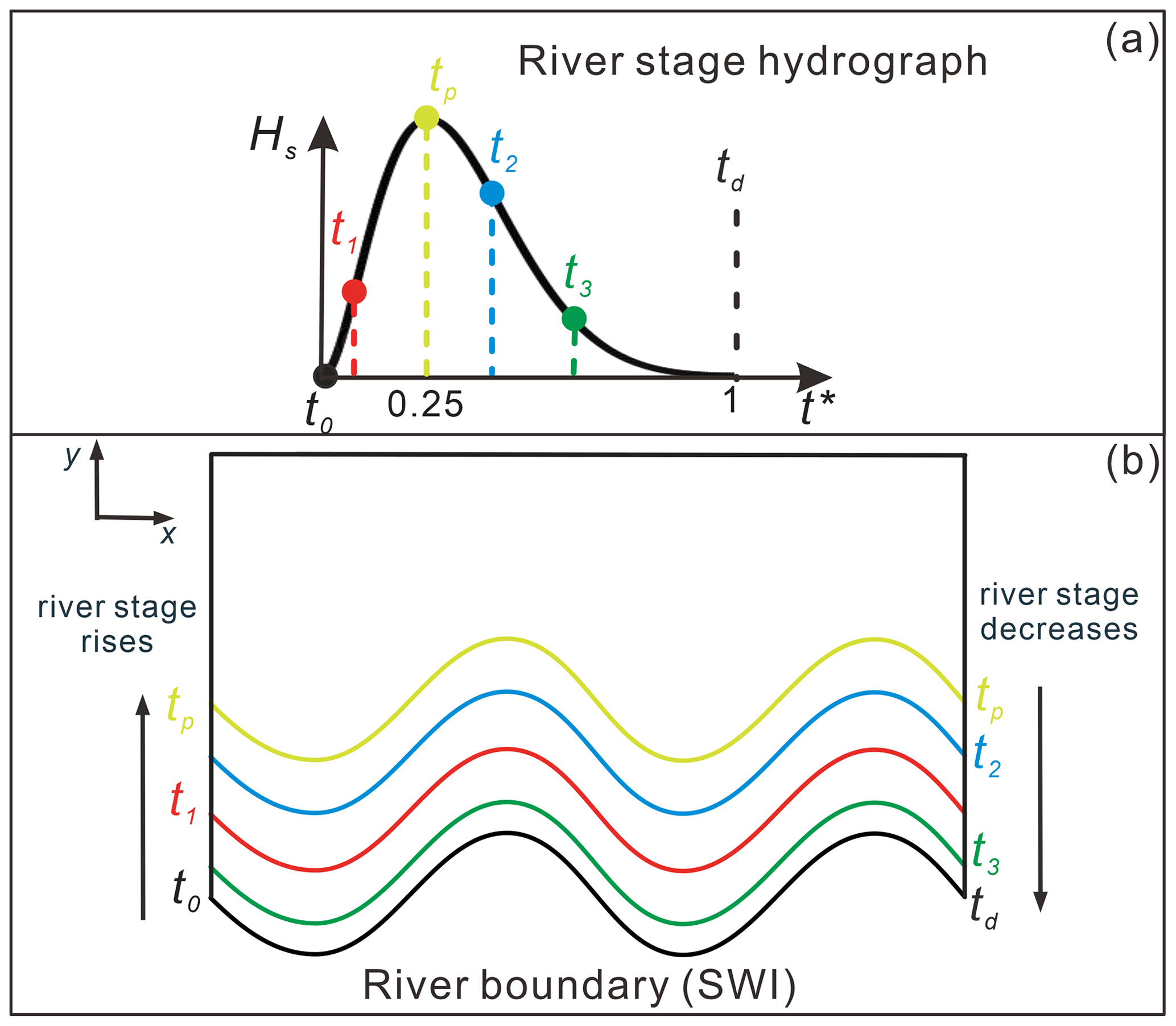
Figure 1 (a) River stage hydrograph during the flood event and (b) diagram showing displacement of the SWI during the flood event. The colored SWIs in (b) correspond to the times of colored dots in (a). When the river stage increases, the river boundary migrates into the aquifer and recovers to its initial location as the river stage decreases, as also indicated by the arrows.

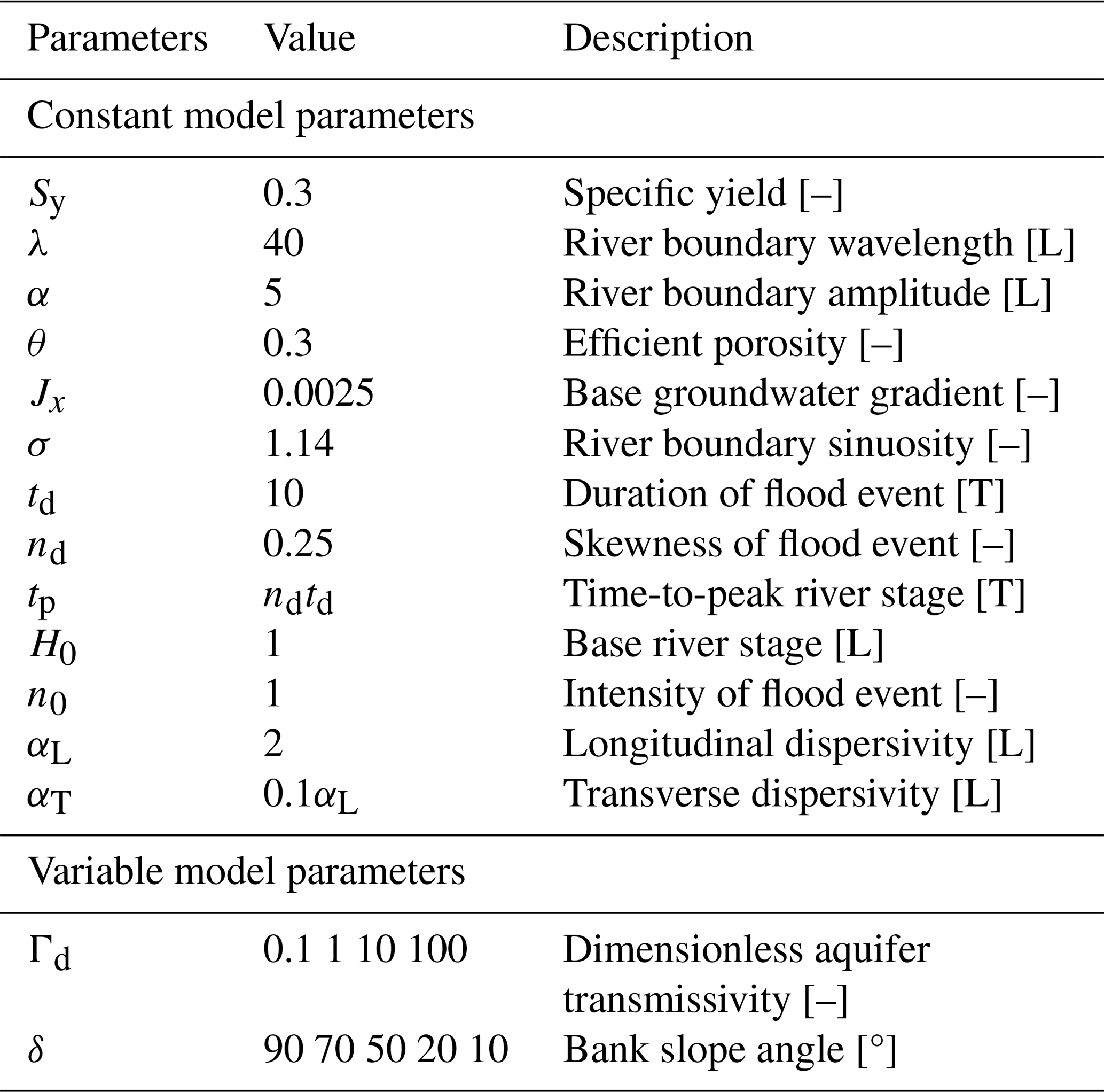
Table 1 Parameters and values used in our numerical model simulations.

2.2 Model parameterization, testing and scenarios

Hydraulic conditions used in our numerical modeling study are based on values from Gomez-Velez et al. (2017), who conducted a Monte Carlo analysis. They found that the dynamic variations of HEF and mean RTD are mainly determined by ambient groundwater flow and the ratio of aquifer hydraulic conductivity to the duration of the flood event, referred to as dimensionless constant $\mathrm{\Gamma }d=\frac{S_{\mathrm{y}}\mathit{\lambda }\mathrm{2}}{\mathrm{0.5}K(\mathrm{1}+n\mathrm{0})H\mathrm{0}{t}_{\mathrm{d}}}$, (see Table 1 and Fig. S2), where S_y is the specific yield [–], λ is the wavelength of the sinuous river, K is the hydraulic conductivity [LT⁻¹], n₀ is the intensity of the flood event [–], H₀ is the base river stage [L] and t_d is the duration of the flood event [T]).

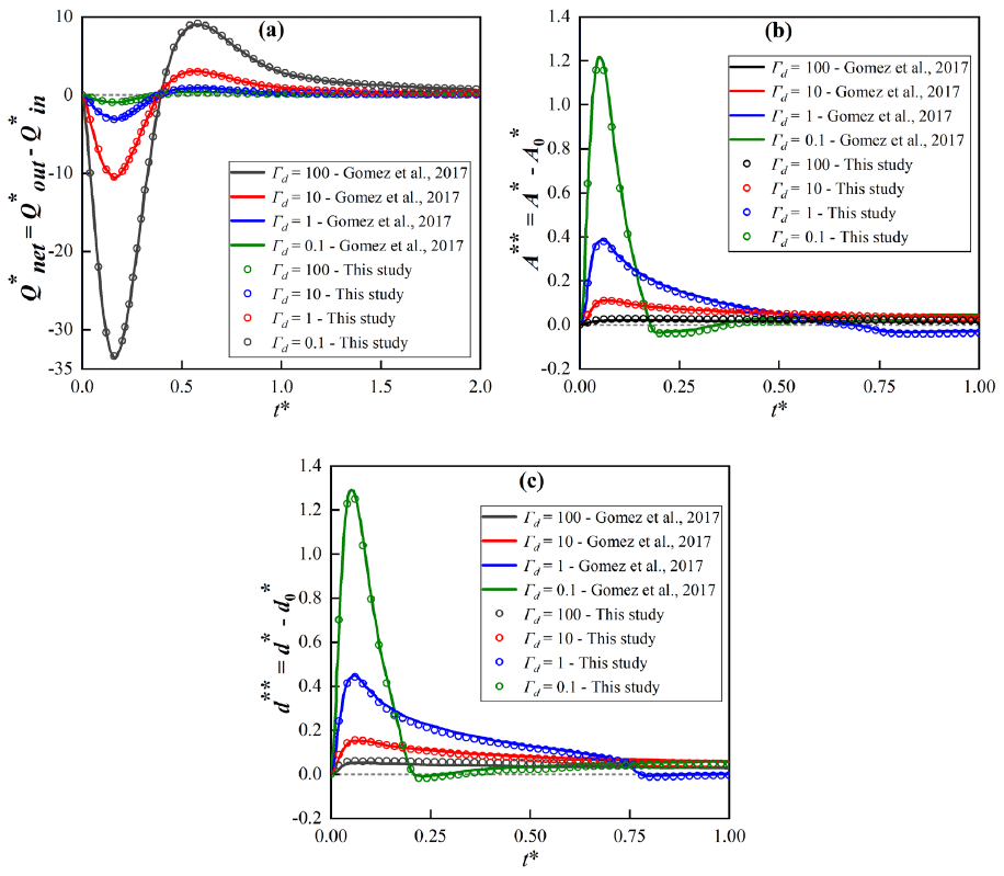
Figure 2 Comparison of results obtained in this study with those of Gomez-Velez et al. (2017) for the baseline case with a vertical riverbank and variable Γ_d: (a) net hyporheic exchange flux represented by $Q_{\text{net, HZ}}^{\ast }\left(t\right)$, (b) extent of the hyporheic zone $A^{\ast \ast }\left(t\right)$ and (c) penetration distance d^∗(t) of the hyporheic zone into the alluvial valley. A more refined mesh and different length scales used in this study can explain slight variations between our model and that of Gomez-Velez et al. (2017). Information regarding model fits can be found in the Supplement.

After setting up the baseline model case with a vertical riverbank (δ = 90°), we compared our model results for that case with those obtained by Gomez-Velez et al. (2017) for (a) net HEF represented by $Q_{\text{net, HZ}}^{\ast }\left(t\right)$; (b) area of HZ, $A^{\ast \ast }\left(t\right)$; and (c) penetration of the HZ, d^∗(t) for Γ_d = 0.1, 1, 10 and 100, and we found that our model simulated those cases with high accuracy (Fig. 2). Parameters $A^{\ast \ast }\left(t\right)$ andd^∗(t) are based on modeling the transport of a conservative solute while $Q_{\text{net, HZ}}^{\ast }\left(t\right)$ is based on modeling water flow. Slight differences between our model and that of Gomez-Velez et al. (2017) might be due to the use of a much more refined mesh in this study as well as different length scales.

To test whether our assumption of considering a vertical SWI and using the DGM to characterize the migration of the SWI was appropriate, we compared the vertical 2-D model with a 1-D model coupled with the DGM. Detailed information on this comparison as well as validation results is provided in Sect. S4 in the Supplement. The results show that our approach is reasonable when simulating HEF in a sloping riverbank aquifer.

We then considered a series of riverbank scenarios where the bank slope angle was varied, ranging from δ = 90° (vertical riverbank) to 10° (nearly horizontal case), and Γ_d values ranged from 0.1 to 100, corresponding to aquifer hydraulic conductivity ranging from 480 to 0.048 m d⁻¹, indicating high to low transmissivity. Table 1 presents the parameters used in our numerical modeling study. The finite-element models proposed in this study were set up using COMSOL software. Equations (S1), (S3) and (S6) in the Supplement were implemented using a customized partial differential equation (PDE) interface to include the Boussinesq equation, vertical integrated solute transport equation and equation for calculating residence (travel) time distributions (RTDs), respectively. The model domain was discretized into about 0.5 million variably sized triangular elements, with refinement imposed near the river boundary. Mesh-independent numerical solutions are achieved by limiting grid size (ΔL) to less than 0.2 m. Thus, the transverse and longitudinal Péclet numbers (calculated by $Pe=\mathrm{\Delta }L/{\mathit{\alpha }}_{\mathrm{L}}$ and $Pe=\mathrm{\Delta }L/{\mathit{\alpha }}_{\mathrm{T}}$, respectively) in both advection- and diffusion-dominated zones are less than 1, which is smaller than the upper limit of Pe = 4 to effectively avoid numerical oscillations and instabilities.

Similar to Gomez-Velez et al. (2017), we evaluated the impact of bank slope by comparing the net hyporheic exchange flux ($Q_{\text{net, HZ}}^{\ast }\left(t\right)$), area of HZ ($A^{\ast \ast }\left(t\right)$), penetration distance of the HZ ($d^{\ast \ast }\left(t\right)$) and mean RTD (${\mathit{\mu }}_r^{\ast }(\mathit{x},t)$) between vertical and sloping riverbank models. A detailed definition of these variables is provided in Sect. S5 in the Supplement.

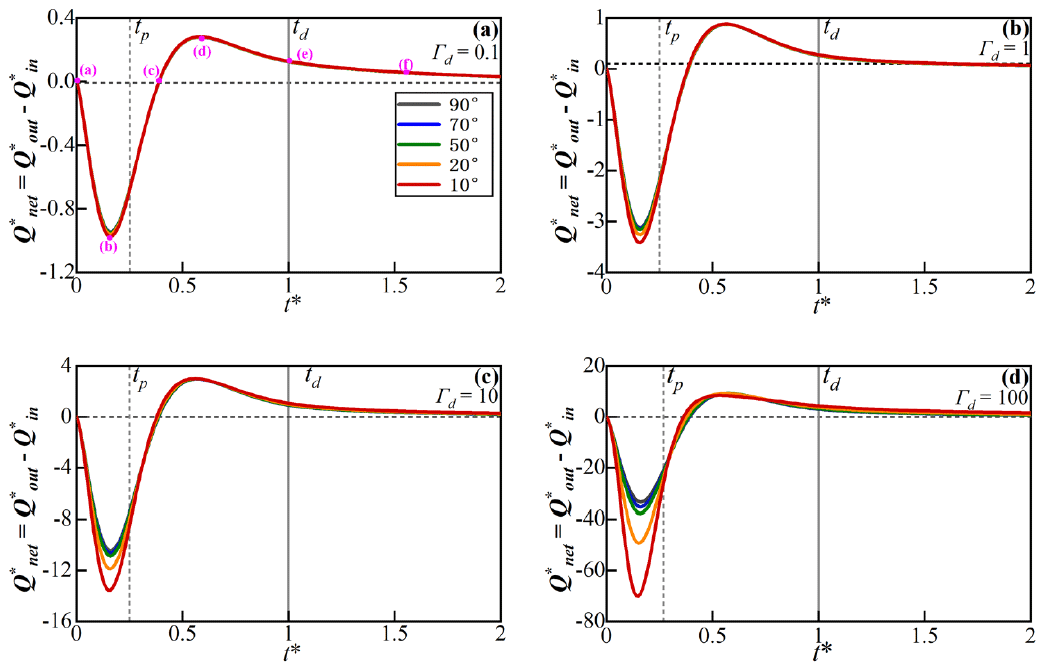
Figure 3 Temporal progression of dimensionless net HEF ($Q_{\text{ne, HZ}}^{\ast }\left(t\right)$) for four different aquifer transmissivity values (represented by Γ_d) and bank slope angles (δ, from 10–90°). Time to peak flood (t_p) and flood duration (t_d) are marked by vertical dashed lines. Pink dots in (a) marked by (a–f) correspond to the snapshots of the flow field shown in Fig. 4. A negative flux value here represents water flow from the river to the aquifer. Note that Γ_d negatively correlates with the transmissivity of the aquifer.

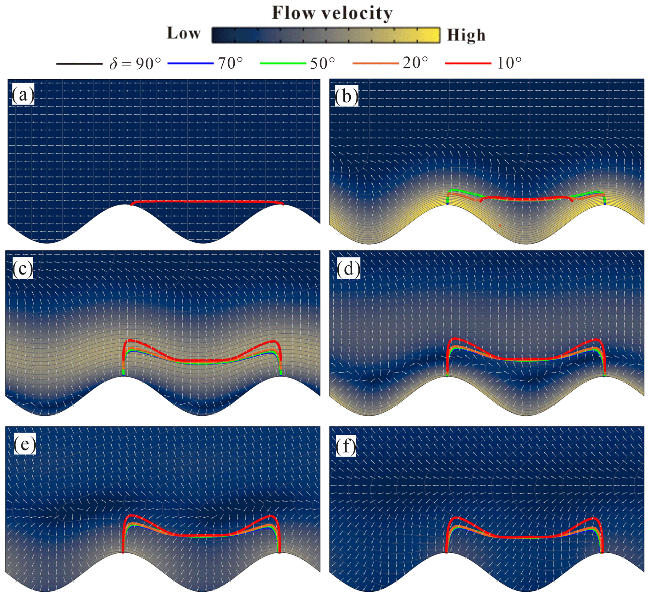
Figure 4 Plan view of the river channel and aquifer, showing the temporal progression of the alluvial flow field and spatial extent of the HZ. Panels (a–e) are snapshots of the flow field at different time steps (t^∗ = 0, 0.16, 0.39, 0.57, 1, 1.5) during the simulated event (pink dots in Fig. 3a). Colored surfaces represent the magnitude of the Darcy flux vector (blue is low, and yellow is high) and white isolines the dimensionless hydraulic head. Bold colored lines correspond to the HZ extent for different bank slope conditions.

3 Results

3.1 Effect of bank slope on hyporheic exchange flow and HZ extent

3.1.1 Hyporheic exchange flow

The flow field (velocity magnitude and direction) and net HEF ($Q_{\text{ne, HZ}}^{\ast }\left(t\right)$) changed dynamically during and after the simulated flood event. Figure 3a–d show the progression of net HEF for different aquifer transmissivity (Γ_d) and bank slope angle (δ) conditions. Snapshots of the flow field and the boundary of the HZ area (isolines of C(x,t) = 0.5 as concentration of a conservative solute) for different δ conditions at different times (pink dots in Fig. 3a) for Γ_d = 1 are shown in Fig. 4a–f.

Before the flood event (t = 0), steady-state base flow conditions are assumed, as shown in Fig. 4a. The inflow and outflow (along the upstream and downstream meander bend, respectively) are in balance. The bank slope has no effect on the HZ boundaries before the flood event. Before the peak river stage of the flood event is reached (0 < t < 0.25t_d), the onset of the flood event is indicated by the rising river stage and forces the river to infiltrate into the aquifer along the SWI (negative values of $Q_{\text{net, HZ}}^{\ast }\left(t\right)$ in Fig. 3), resulting in the expansion of the HZ as shown in Fig. 4b. The influx of river water into the HZ ($-Q_{\text{ne, HZ}}^{\ast }\left(t\right)$) reaches its maximum before the time-to-peak river stage (t = 0.25t_d) because the pressure wave propagates into the aquifer and decreases the head gradient between the river and the connected aquifer. For higher-transmissivity aquifers (lower Γ_d values in Fig. 3), the bank slope has a reduced impact on net outflux as the fast propagation of the pressure wave results in the hydraulic head near the SWI to be very similar. Among different aquifer transmissivity conditions, as aquifer transmissivity decreases, the ability of the aquifer to transmit the pressure wave becomes limited, and the interaction flux is dominated by the location (displacement) of the SWI and the river stage. On the other hand, a smaller slope angle induces a longer displacement of the SWI (M(t)) away from the river, where the groundwater head adjacent to the SWI is always relatively high (i.e., the head in base flow condition). This, consequently, leads to a larger head gradient near the SWI as well as larger dimensionless net fluxes under increasing Γ_d conditions as shown in Fig. 3.

The maximum dimensionless flux ratios $Q_{\text{max, var}}^{\ast }$ = $Q_{\text{max, s}}^{\ast }/Q_{\text{max, v}}^{\ast }$ of sloping (δ < 90°, $Q_{\text{max, s}}^{\ast }$) vs vertical (δ = 90°, $Q_{\text{max, v}}^{\ast }$) riverbank cases are shown in Fig. 5, which indicates the deviation in predicting peak net flux when neglecting the slope of the riverbank. The bank slope is found to increase infiltration by up to 120 % ($Q_{\text{max, var}}^{\ast }\approx \mathrm{2.2}$) for Γ_d = 100 with δ = 10°, while for larger slope angles or higher hydraulic transmissivities the dimensionless infiltration gradually decreases.

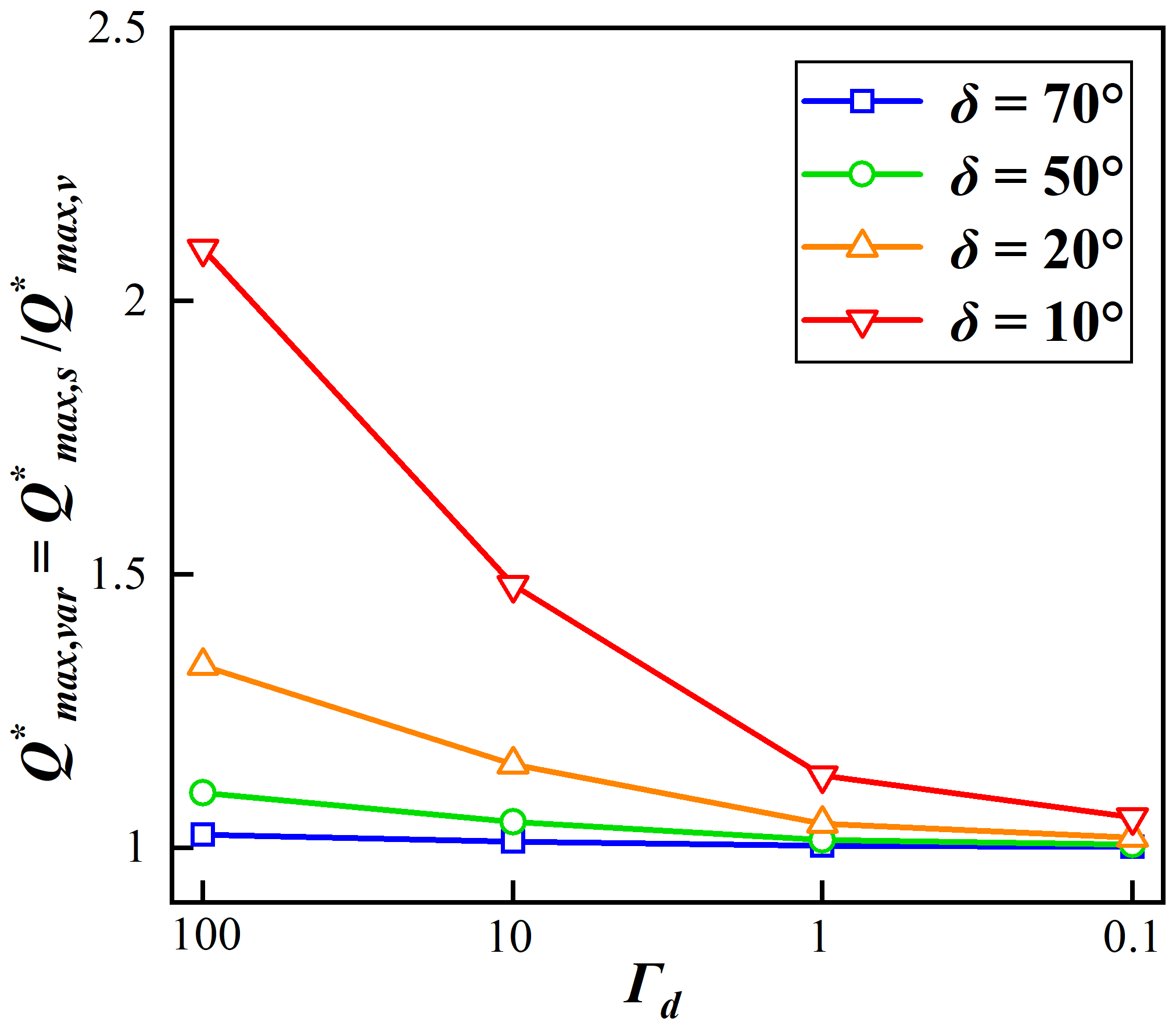
Figure 5 Ratio of maximum net flux for slope to no-slope (vertical riverbank) conditions $Q_{\text{max, var}}^{\ast }=Q_{\text{max, s}}^{\ast }/Q_{\text{max, v}}^{\ast }$ for four aquifer transmissivities and slope angles. Note that Γ_d negatively correlates with aquifer transmissivity.

As the river stage decreases after t_p, the head gradient near the SWI gradually reverses, and the net outflux starts increasing (the river is gaining water), as shown in Fig. 3. This is associated with the river stage declining below the groundwater level (see Fig. 4c–f). For the lowest hydraulic transmissivity condition (Γ_d = 100), bank slope can slightly extend the time required for the system to recover to initial conditions after t_p, but in general, the response of the net outflux to bank slope is negligible when compared to that of the influx. Eventually, the net flux converges to zero, which indicates the flow field within the aquifer recovers to the initial conditions. The bank slope has no impact on the HEF after the duration of the flood event.

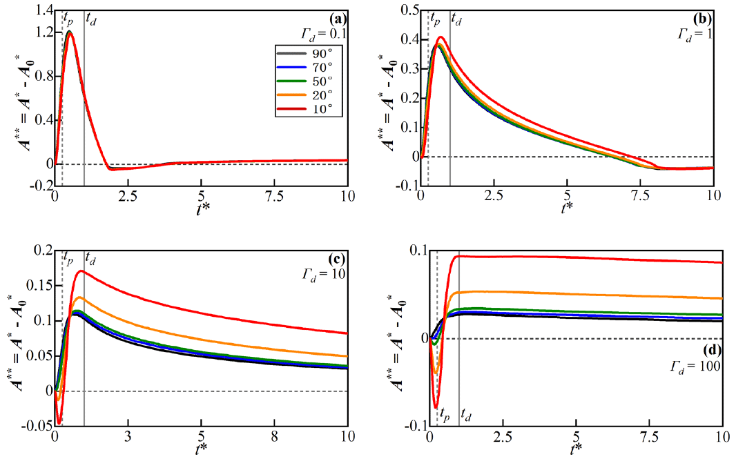
Figure 6 Temporal progression of dimensionless HZ area for different values of Γ_d and δ (colored lines). Time to peak (t_p) and flood duration (t_d) are marked by vertical dashed lines.

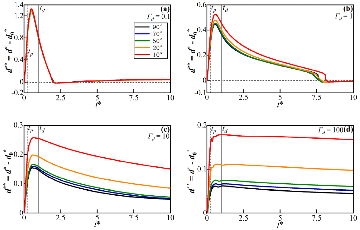
Figure 7 Temporal progression of dimensionless HZ penetration distance into the alluvial valley ($d^{\ast \ast }$) for different values of Γ_d and δ (colored lines). Time to peak (t_p) and flood duration (t_d) are marked by vertical dashed lines.

3.1.2 Patterns of hyporheic area and penetration distance

Figures 6 and 7 show the temporal progression of the dimensionless HZ area ($A^{\ast \ast }\left(t\right)$) and penetration distance ($d^{\ast \ast }\left(t\right)$) into the alluvial valley relative to the initial condition for varying aquifer transmissivity (Γ_d) and slope angles.

For vertical banks (δ = 90°, black lines in Fig. 6), the HZ area increases synchronously with the river stage (t < t_p). After the peak time of the flood event (t > t_p), the HZ area continues to extend as river water still recharges the aquifer. After the flood event (t > t_d), the river water that was stored in the aquifer (C(x,t) > 0) slowly discharges back into the river channel. Thus, the HZ area and penetration distance gradually rebound to initial conditions.

Under sloping riverbank conditions, the riverbank will at times be submerged by the rising river stage. Figures 6a and 7a show that the effects of bank slope on HZ area ($A^{\ast \ast }\left(t\right)$ in Fig. 6) and penetration distance ($d^{\ast \ast }\left(t\right)$ in Fig. 7) are almost counteracted by the high transmissivity of the aquifer while the influence of the bank slope was negligible. At the beginning of the flood event, Fig. 6b–d show that for conditions with a smaller sloping angle, the HZ area can be less than zero (HZ at these times is smaller than the initial condition). This is due to the fact that the movement of the SWI during a rising river stage towards the alluvial valley will submerge parts that were previously unsaturated as the aquifer with low transmissivity will propagate water more slowly. As aquifer transmissivity decreases from Fig. 6b–d, the relative HZ area remains negative for a longer time for smaller bank slopes. This indicates that bank slope has a more pronounced effect on HZ extent in cases where aquifer transmissivity is large as a low-transmissivity aquifer takes more time to propagate infiltrating river water.

After about half the flood duration (t > 0.5t_d), the HZ area ($A^{\ast \ast }$) becomes positive in all scenarios as the model domain previously submerged during the flood event re-emerges. As aquifer transmissivity decreases (Figs. 6a–d and 7a–d), the impact of bank slope gradually increases, especially in low aquifer transmissivity conditions, where a smaller bank slope can increase the peak values of area and penetration distance and delay the arrival time-to-peak value of the relative HZ area. After the flood event (t > t_d), the effect of the bank slope is counteracted by the higher aquifer transmissivity, and only lower transmissivities have a significant impact on the HZ, resulting in larger $A^{\ast \ast }\left(t\right)$ and $d^{\ast \ast }\left(t\right)$ as shown in Figs. 6b–d and 7b–d. For low-transmissivity scenarios, the bank slope can increase the peak area and penetration of the HZ by almost 200 %.

3.2 Spatiotemporal progression of mean residence time distribution

The progression of spatiotemporal patterns of mean RTD (i.e., travel time of river water in aquifer) is a useful evaluation method for identifying the dynamic variation of aging and rejuvenation of hyporheic water. Here we use the mean RT ratio between a sloping model and a vertical model ${\mathit{\mu }}_r^{\ast }(\mathit{x},t)$ = ${\text{log}}_{\mathrm{10}}\left({\mathit{\mu }}_{\mathit{\tau }-S}\right(\mathit{x},t)/{\mathit{\mu }}_{\mathit{\tau }-V}(\mathit{x},\mathrm{0}\left)\right)$ to evaluate the influence of bank slope on the prediction of mean RTD for a given location and time. Figure 8 presents mean RTDs for the initial condition, where ${\mathit{\mu }}_{\mathit{\tau }\mathrm{0}-max}$ is the maximum RT in the domain. It can be seen that the isolines representing the RT are almost horizontal in the area extending from the river, but RT near the upstream river bend is smaller than downstream because the initial flow direction is towards the negative direction of the x axis. Notably, μ(x,0) grows almost exponentially as y increases, and a positive correlation to Γ_d at a given location is observed.

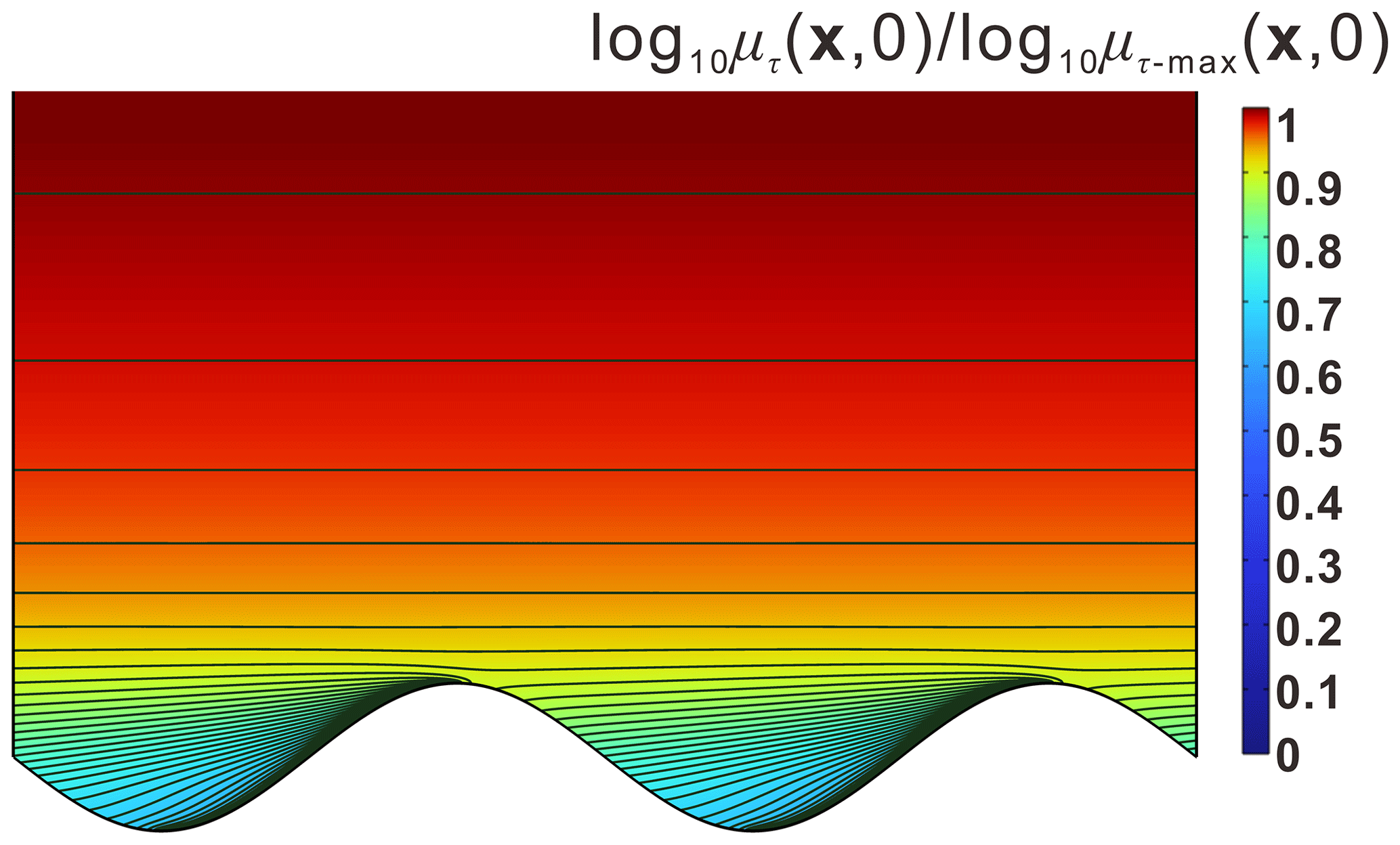
Figure 8 Plan view of relative mean residence time distributions [–] for baseline flow conditions (no bank slope), which are represented by ${\text{log}}_{\mathrm{10}}{\mathit{\mu }}_{\mathit{\tau }}(\mathit{x},\mathrm{0})/{\text{log}}_{\mathrm{10}}{\mathit{\mu }}_{\mathit{\tau }-\text{max}}(\mathit{x},\mathrm{0})$ to show the distribution pattern. The value of the contour lines grows exponentially with the distance from the river meander.

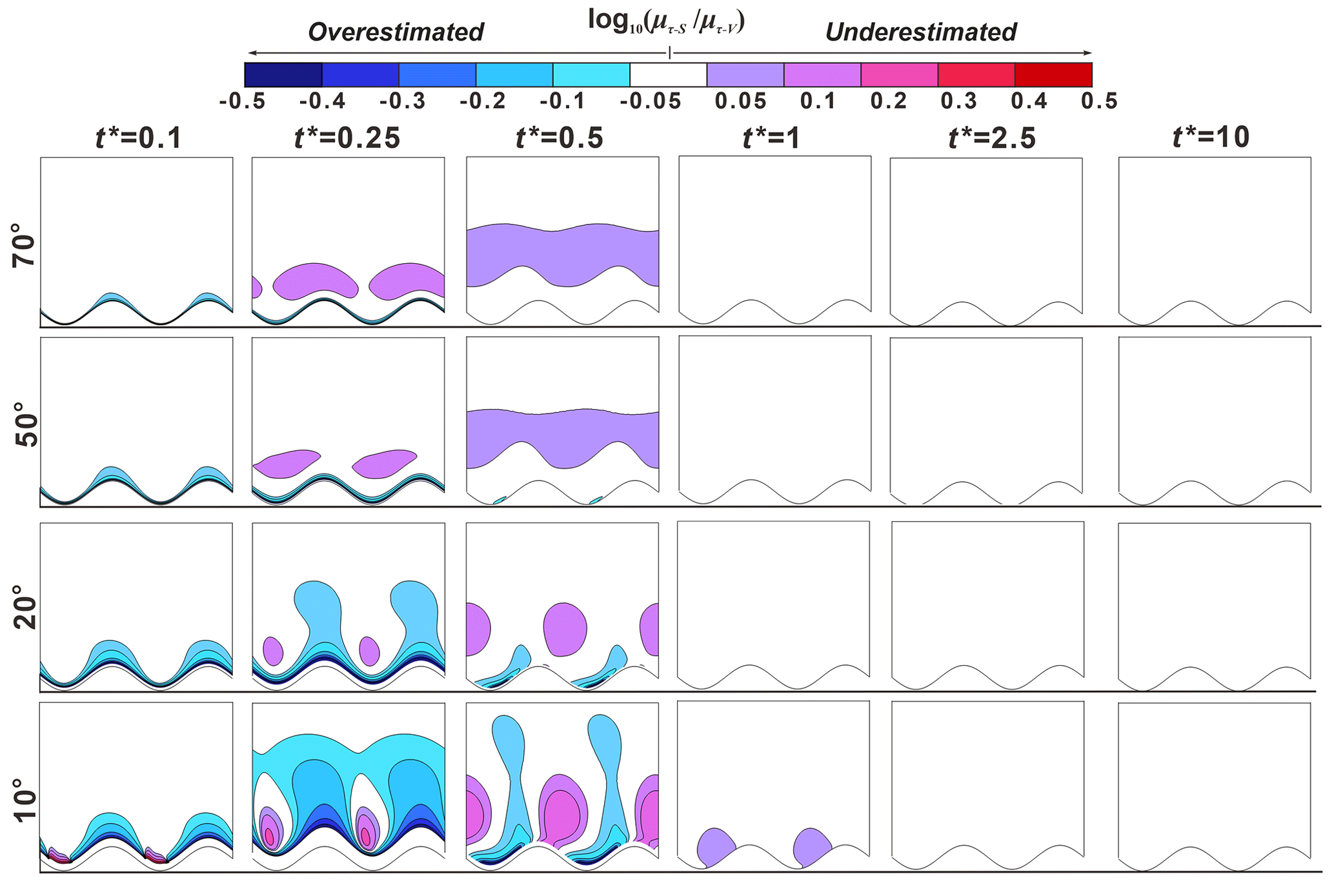
Figure 9 Five snapshots for the mean RTD ratio (${\mathit{\mu }}_r^{\ast }(\mathit{x},t)={\mathit{\mu }}_{r-S}^{\ast }(\mathit{x},t)/{\mathit{\mu }}_{r-V}^{\ast }(\mathit{x},t)$) between sloping (${\mathit{\mu }}_{r-S}^{\ast }(\mathit{x},t)$) and vertical riverbank conditions (${\mathit{\mu }}_{r-V}^{\ast }(\mathit{x},t)$) at different times t^∗ as a function of δ for Γ_d = 0.1. The horizontal lines beneath each figure are the reference lines to show the initial location of the peak point of the point bar. The lower sinuous lines at the reference lines are the initial SWIs. The colored areas indicate where the bank slopes have a significant impact on RT (difference in RT between sloping and vertical model larger than 12.2 %) and residence (travel) times of river water in the aquifer would be overestimated (cold-color area) or underestimated (warm-color area) if the effect of the bank slope was ignored.

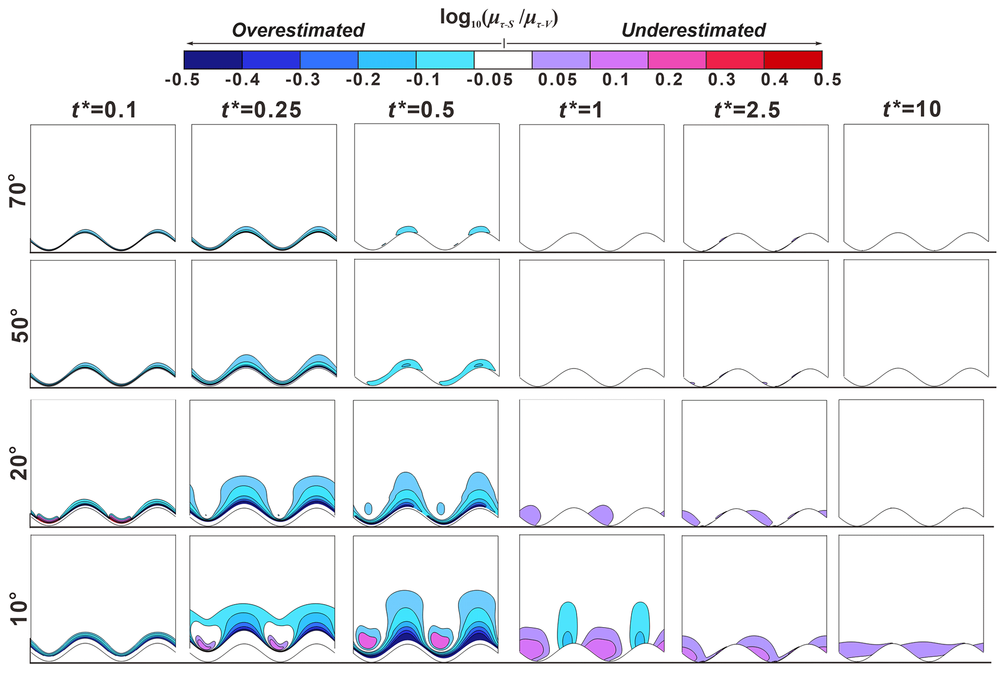
Figure 10 Five snapshots for the mean RTD ratio (${\mathit{\mu }}_r^{\ast }(\mathit{x},t)={\mathit{\mu }}_{r-S}^{\ast }(\mathit{x},t)/{\mathit{\mu }}_{r-V}^{\ast }(\mathit{x},t)$) between sloping (${\mathit{\mu }}_{r-S}^{\ast }(\mathit{x},t)$) and vertical riverbank conditions (${\mathit{\mu }}_{r-V}^{\ast }(\mathit{x},t)$) at different times t^∗ as a function of δ for Γ_d = 1. The horizontal lines beneath each figure are the reference lines to show the initial location of the peak point of the point bar. The lower sinuous lines at the reference lines are the initial SWIs. The colored areas indicate where the bank slopes have a significant impact on RT (difference in RT between sloping and vertical model larger than 12.2 %) and residence (travel) times of river water in the aquifer would be overestimated (cold-color area) or underestimated (warm-color area) if the effect of the bank slope was ignored.

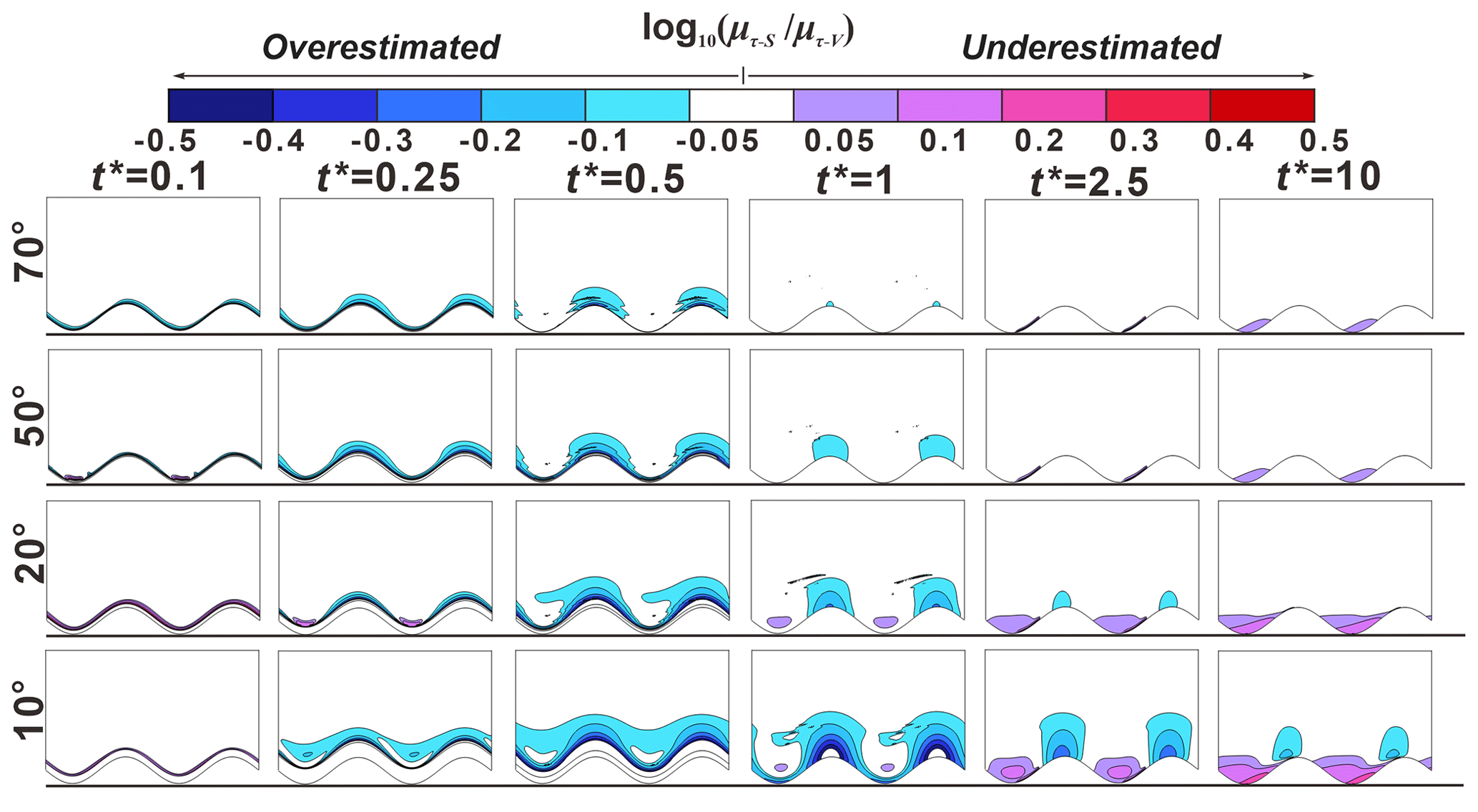
Figure 11 Five snapshots for the mean RTD ratio (${\mathit{\mu }}_r^{\ast }(\mathit{x},t)={\mathit{\mu }}_{r-S}^{\ast }(\mathit{x},t)/{\mathit{\mu }}_{r-V}^{\ast }(\mathit{x},t)$) between sloping (${\mathit{\mu }}_{r-S}^{\ast }(\mathit{x},t)$) and vertical riverbank conditions (${\mathit{\mu }}_{r-V}^{\ast }(\mathit{x},t)$) at different times t^∗ as a function of δ for Γ_d = 10. The horizontal lines beneath each figure are the reference lines to show the initial location of the peak point of the point bar. The lower sinuous lines at the reference lines are the initial SWIs. The colored areas indicate where the bank slopes have a significant impact on RT (difference in RT between sloping and vertical model larger than 12.2 %) and residence (travel) times of river water in the aquifer would be overestimated (cold-color area) or underestimated (warm-color area) if the effect of the bank slope was ignored.

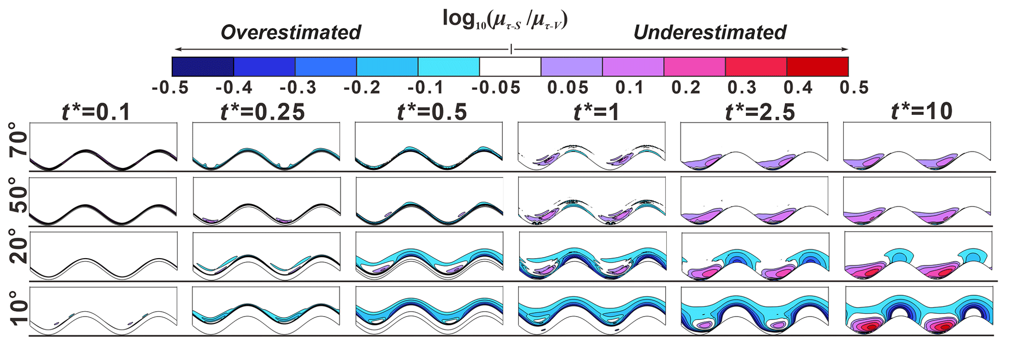
Figure 12 Five snapshots for the mean RTD ratio (${\mathit{\mu }}_r^{\ast }(\mathit{x},t)={\mathit{\mu }}_{r-S}^{\ast }(\mathit{x},t)/{\mathit{\mu }}_{r-V}^{\ast }(\mathit{x},t)$) between sloping (${\mathit{\mu }}_{r-S}^{\ast }(\mathit{x},t)$) and vertical riverbank conditions (${\mathit{\mu }}_{r-V}^{\ast }(\mathit{x},t)$) at different times t^∗ as a function of δ for Γ_d = 100. The horizontal lines beneath each figure are the reference lines to show the initial location of the peak point of the point bar. The lower sinuous lines at the reference lines are the initial SWIs. The colored areas indicate where the bank slopes have a significant impact on RT (difference in RT between sloping and vertical model larger than 12.2 %) and residence (travel) times of river water in the aquifer would be overestimated (cold-color area) or underestimated (warm-color area) if the effect of the bank slope was ignored.

Figures 9–12 present five snapshots of ${\mathit{\mu }}_r^{\ast }$ for different bank slope angles and different aquifer transmissivity values (Γ_d = 0.1, 1, 10 and 100, respectively). The five snapshots represent the rising limb of the flood event ($t^{\ast }=\mathrm{0.1}$), the peak of the flood event ($t^{\ast }=\mathrm{0.25}$), the falling limb of the flood event ($t^{\ast }=\mathrm{0.5}$) and a time after the flood event ($t^{\ast }=\mathrm{1}$, 2.5 and 10). The differences in residence time between sloping and vertical riverbank models are within 12.2 % in the white-colored areas (−0.05 < ${\mathit{\mu }}_r^{\ast }$ < 0.05) of Figs. 9–12, which indicates a minor effect of bank slope on mean RTD. The colored areas in Figs. 9–12 indicate model results where neglecting the bank slope will lead to an overestimation (${\mathit{\mu }}_r^{\ast }$ < −0.05) or underestimation (${\mathit{\mu }}_r^{\ast }$ > 0.05) of residence (travel) times.

At $t^{\ast }=\mathrm{0.1}$, a smaller bank slope can lead to a shorter travel time of river water in the aquifer (negative values of ${\mathit{\mu }}_r^{\ast }$) near the SWI compared to the vertical riverbank scenario. The area of shorter travel time caused by bank slope was positively related to aquifer transmissivity. The effect of bank slope is small for Γ_d = 10 and 100 because the groundwater mound (the raised groundwater stage) piles up around the river boundary, but that small area extended deeper into the alluvial valley for smaller slope angles. Due to the scattered and nested flow paths near the cut bank and point bar, respectively, the area of the negative value of ${\mathit{\mu }}_r^{\ast }$ at the cut bank of the SWI is larger than that at the point bar. The change of flow direction near the point bar leads to a prolonged flow path for the water in the river channel as well as to forced groundwater mixing with the slightly older water (Fig. 8 shows that the water was potentially older in the y direction compared to the −x direction in the point bar). This effect was amplified with decreasing the bank slope angle, but it is only statistically significant (${\mathit{\mu }}_r^{\ast }$ < −0.05 or ${\mathit{\mu }}_r^{\ast }$ > 0.05) when δ = 10° at $t^{\ast }=\mathrm{0.1}$.

At the time of peak flood ($t^{\ast }=\mathrm{0.25}$), the river still infiltrates into the aquifer. For Γ_d = 0.1, results of ${\mathit{\mu }}_r^{\ast }$ in Figs. 9 show that the bank slope can lead to both overestimated and underestimated RT areas. Both the magnitude of relative RT (${\mathit{\mu }}_r^{\ast }$) and the associated area increase with a decreasing slope due to the longer travel distance of river water into the aquifer. As the slope angle decreases, the underestimated travel time area was located closer to the peak of the cutbank. The impact of bank slope on mean RTD for Γ_d = 1 was rather similar in its pattern compared to Γ_d = 0.1, but the degree of that impact was reduced. For Γ_d = 10 and 100, only overestimated travel time area can be seen near the riverbank with a smaller area of impact compared to smaller Γ_d conditions because the groundwater has not sufficiently propagated into the aquifer due to lower transmissivity.

At $t^{\ast }=\mathrm{0.5}$, part of the aquifer that was submerged at $t^{\ast }=\mathrm{0.25}$ reemerges due to the decline in river stage. In most cases, smaller bank slopes can lead to wider reemergence of the aquifer, which therefore results in overestimated travel time area near the river boundary; however, this was not the case for Γ_d = 0.1, where the bank slope can lead to both an overestimated and an underestimated RT area. Furthermore, compared to when $t^{\ast }=\mathrm{0.25}$, the impact of bank slope becomes weaker for Γ_d = 0.1 but more relevant for the larger Γ_d values.

After the flood event (t^∗ > 1), the influence of bank slope on mean travel time is nearly eliminated for Γ_d = 0.1 and 1 due to the high aquifer transmissivity. However, for aquifers with lower transmissivity (Γ_d = 10 and 100), bank slope still has a significant effect on RT at $t^{\ast }=\mathrm{10}$ and leads to underestimated and overestimated RT areas near the point bar and the cut bank, respectively.

Overall, Figs. 9–12 indicate that the time when bank slope was relevant in predicting RT (travel time of groundwater in aquifer) was determined by the transmissivity of the aquifer. For more transmissive aquifers, the impact of bank slope on the prediction of groundwater travel time cannot be neglected during the flood event (0 < t < t_d), but that impact will be eliminated after the flood event due to the quick recovery of the aquifer to baseline conditions. For lower-transmissivity aquifers, the bank slope plays an important role in groundwater travel time after t > 0.5^∗t_d and has a more lasting influence on aquifer RT, as more time is required to recover to initial conditions.

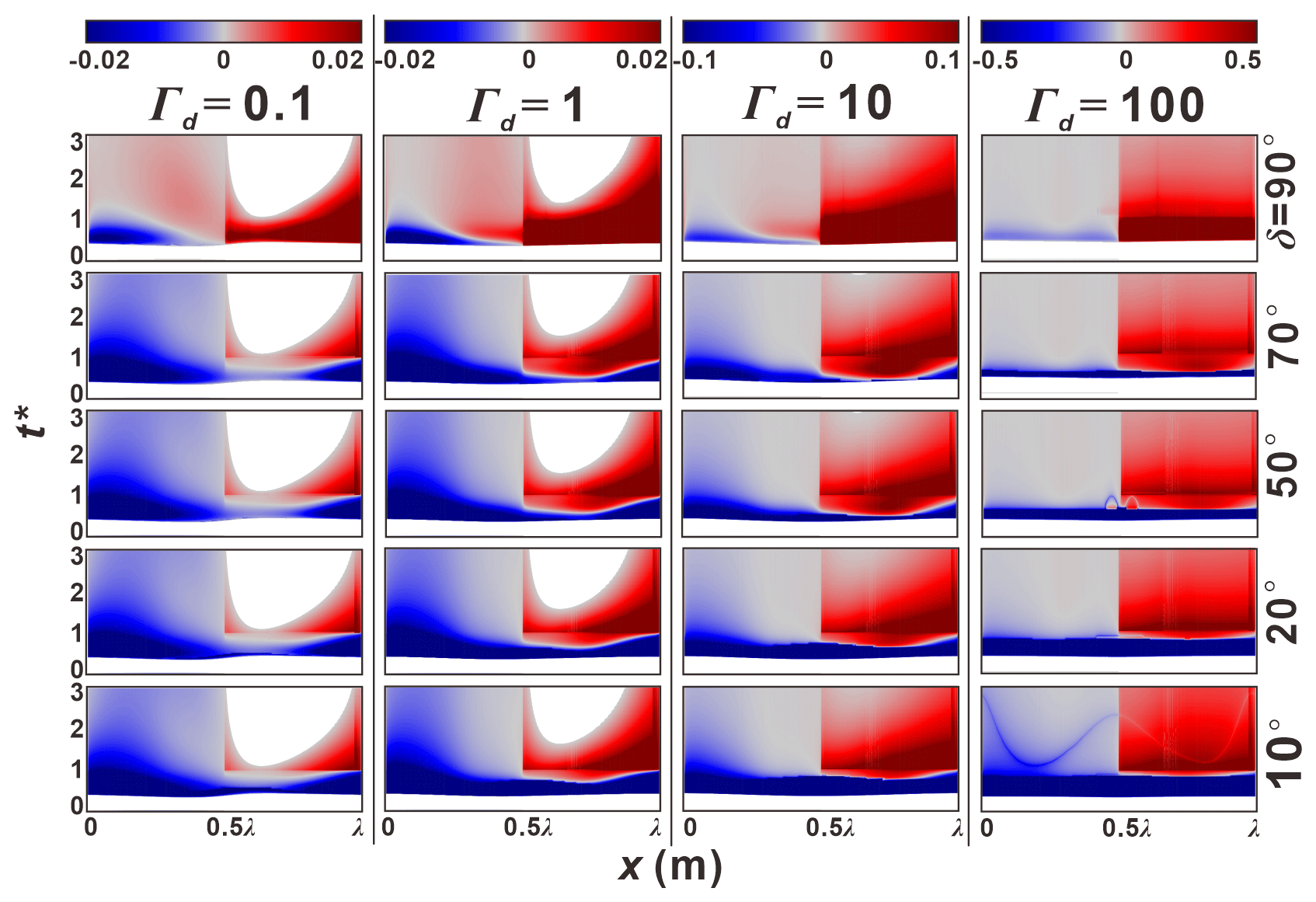
Figure 13 Temporal progression of flux-weighted ratios of RT to the RT for baseline conditions (${\mathit{\mu }}_{\text{out}}^{\ast }(x,t)=n\cdot Q_{\text{out}}^{\ast }(x,t){\text{log}}_{\mathrm{10}}\left({\mathit{\mu }}_{\mathit{\tau }}\right(x,t)/{\mathit{\mu }}_{\mathit{\tau }}(x,\mathrm{0}\left)\right)$) along the river meander as a function of δ and Γ_d. ${\mathit{\mu }}_{\text{out}}^{\ast }(x,t)$ indicates the difference of flux weighted water RT (travel time) that the aquifer discharges into river compared to the initial condition.

3.3 Relative flux-weighted residence time

Figures 13 shows the progression of the flux-weighted relative RT ${\mathit{\mu }}_{\text{out}}^{\ast }(x,t)$ = $n\cdot Q_{\text{out}}^{\ast }(x,t){\text{log}}_{\mathrm{10}}\left({\mathit{\mu }}_{\mathit{\tau }}\right(x,t)/{\mathit{\mu }}_{\mathit{\tau }}(x,\mathrm{0}\left)\right)$ for different slopes and aquifer transmissivities. $M_{\text{out}}^{\ast }(x,t)$ represents the difference in flux-weighted RT of the water discharged into the river compared to the initial condition. At the start of the flood event, there is no ${\mathit{\mu }}_{\text{out}}^{\ast }$ as river water infiltrates the aquifer. Following the decline in river stage, the aquifer begins to discharge the mixed water with different RT back into the river (see Fig. 4c).

For vertical riverbank conditions (δ = 90°, top row in Fig. 13), upstream (0.5λ < x < λ) and downstream (0 < x < 0.5λ) boundaries of the meander bend discharge older and younger water, respectively. The rejuvenated or aged waters that represent shorter and longer travel times compared to the baseline condition, respectively, were mostly discharged before the flood event (t^∗ < 1) due to the greater outflux as shown in Fig. 3a. It can also be seen that water was aged along the upstream bend compared to the more rejuvenated water along the downstream bend. After the flood event, ${\mathit{\mu }}_{\text{out}}^{\ast }$ gradually disappears along the upstream meander (blank areas) for Γ_d = 0.1 and 1 because the flow fields were recovering to baseline conditions. Therefore, the upstream meander gradually becomes the inflow boundary.

For cases with lower values of Γ_d (left columns in Fig. 13), ${\mathit{\mu }}_{\text{out}}^{\ast }$ reaches equilibrium earlier compared to cases with higher Γ_d as an increasing bank slope angle causes ${\mathit{\mu }}_{\text{out}}^{\ast }$ to gradually decrease the travel time of the outflowing water during the flood event. For larger Γ_d, ${\mathit{\mu }}_{\text{out}}^{\ast }$ was totally dominated by rejuvenated water during the flood event. Furthermore, smaller bank slope angles can both extend the time that younger water is discharging along the downstream meander and increase the difference in residence times of these younger waters between sloping and vertical conditions.

4 Discussion

4.1 Why we should account for the bank slope

Tilted riverbanks are common in nature and caused by erosion and bank collapse, as has been observed at multiple scales (Zingg, 1940). Previous studies have shown that bank erosion is stronger where the river planimetry is more sinuous, the river stage varies more frequently, or where the riverbank has larger sloping angles, ultimately leading to a flatter bank (Zingg. 1940; Haggerty and Gorelick, 1995; Mayor et al., 2008; Puttock et al., 2013). Yet, the impact of riverbank geometry and in particular the bank slope on sinuosity-driven lateral hyporheic exchange was ignored in most previous studies. Our results clearly indicate that HZ characteristics (HEF, area and penetration distance of HZ into the alluvial valley) can be underestimated along a meandering river depending on bank slope conditions.

We show that not accounting for the bank slope and river sinuosity can lead to an underestimation of the infiltration rate of water from the river to the alluvial aquifer (by up to 120 %), as well as the area and penetration distance. This effect is more pronounced for smaller bank slope angles (Fig. 5), which can be more likely found in lowland streams (Laubel et al., 2003), especially in areas with extensive cattle grazing at the streamside (Trimble, 1994).

Doble et al. (2012b), Siergieiev et al. (2015) and Liang et al. (2018) assessed the influence of the bank slope on HEF using a vertical cross-sectional profile. Siergieiev et al. (2015) found that the impact of bank slope on HEF was proportional to the hydraulic conductivity of the aquifer. However, we argue here that the bank slope is more relevant in rivers connected to aquifers with low hydraulic transmissivity (high hydraulic conductivity or low specific yield). Furthermore, we show (Fig. 14 as example) that using only one cross-sectional river profile perpendicular to the river axis does not capture the effect of river sinuosity on HEF as bank storage decreases from point bar to cut bank. This indicates that the accuracy of bank storage estimates can be improved by including river sinuosity, which has often been omitted in the past. In a meandering river with variable bank slope, river geometry thus has a sizable effect on bank storage progression and HEF and should be included in any scenarios.

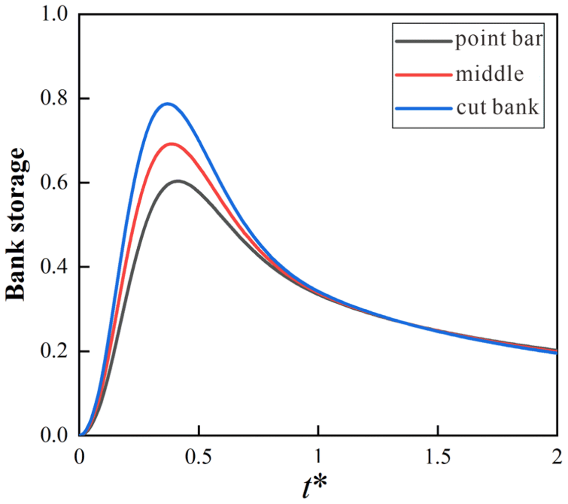
Figure 14 Bank storage versus time for Γ_d = 1 and δ = 90° condition at the peak of the point bar (x = 0), the middle (x = 0.25λ) and the peak of the cut bank (x = 0.25λ). Dimensionless bank storage was calculated by $\frac{{\int }_{Y(x,t)}^{Y(x,t)+\mathrm{4}\mathit{\lambda }}[h-z_b-H_{\mathrm{0}}]\mathrm{d}y}{\mathit{\lambda }{H}_{\mathrm{p}}}$.

4.2 Implications of bank slope on biogeochemical reactions

Under rather stable flow conditions, hyporheic exchange rate and river sinuosity control the biogeochemical zonation (RTD) in the HZ. A higher hyporheic exchange rate (caused, e.g., by a larger hydraulic conductivity in the aquifer or a more sinuous meander) will reduce the mean RTD, promoting biogeochemical reactions (Boano et al., 2010a; Gomez-Velez et al., 2012). However, for a transient flood event, the mean RTD could be both extended and reduced depending on the location with respect to the meander, due to variations in the complex flow paths (Gomez-Velez et al., 2017). Our results indicate that smaller bank slope angles could not only increase HEF and thus lead to increased transport of oxygen and nutrient rich stream water into the aquifer but also alter the location and the residence time of this water within the aquifer system.

Mean RTDs of river water in the alluvial aquifer have been used to evaluate the potential for biogeochemical reactions by comparing the RT with biogeochemical timescales (BTSs) for given solutes (Boano et al., 2010b; Gomez-Velez et al., 2012). Locations where the ratio of RT to BTS (expressed by Damköhler numbers) is small indicate a high reaction potential for that specific chemical species (Gomez-Velez et al., 2015; Pinay et al., 2015). It has been documented that the BTS for dissolved organic matter (DOC) can vary over 10 orders of magnitude (10⁻¹–10⁹ d) (Hunter et al., 1998), while the BTS for oxygen and nitrate has been found to vary over 8 orders of magnitude (10⁻²–10⁶ d) (Gomez-Velez et al., 2012). Here, we compare mean RTD within the overlapping ranges of these two BTS for vertical and sloping riverbank conditions (δ = 10°) at the peak time of the flood event (t^∗ = 0.25) for different aquifer transmissivity conditions and show the zonation of residence times using a BTS range of 10⁻¹–10⁶ d (Fig. 15).

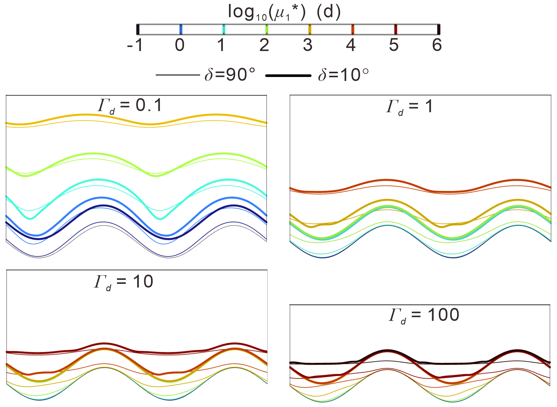
Figure 15 Plan view of the zonation of biogeochemical timescales (BTS, range of 10⁻¹–10⁶) for common HZ constituents such as DOC, oxygen or nitrate for different aquifer transmissivities at t^∗ = 0.25. Thick and thin lines indicate the comparison of vertical vs sloping riverbank (δ = 10°) conditions, while the different colors indicate the different exponents. Unlike the previous mean RTD figures in which relative mean RTD is expressed in dimensionless form, the spatial scales of mean RTD in this figure are dimensional in days.

Figure 15 indicates that neglecting the bank slope impacts the prediction of reaction potentials during hyporheic exchange processes, especially for locations with short timescales. The reaction hot spots (areas indicated by the overlapping BTS ranges) for sloping riverbank conditions expanded further into the aquifer compared with the vertical bank conditions, similar to the overestimated areas in Figs. 9 to 12. Note that we did not aim to include specific reaction models in our study but instead used mean RTD as an indicator for various biogeochemical reactions in the aquifer. Furthermore, the wavelength of the river sinusoid in Fig. 15 was λ = 40 m to offer a representative riverbank–aquifer condition. The zonation of BTSs for larger and smaller river sinusoid wavelengths will be reduced towards the river boundary or further expanded into the aquifer, respectively, for both sloping and vertical riverbank conditions. Although the dimensional BTSs for various spatial scales are not shown here, similar patterns between Figs. 9–12 and 15 imply the usability of the mean RTD results (Figs. 9–12) to infer potential biogeochemical reactions.

The impact of the bank slope on RT is basically controlled by aquifer transmissivity. For higher aquifer transmissivity conditions, the impact of the bank slope appears to be more pronounced when the river stage rises during a flood event. For lower aquifer transmissivity conditions, the bank slope seems more relevant for mean RTD after the flood event, and its impact is more long-lasting. Smaller bank slope angles could extend (near the point bar) or reduce (near the cut bank) pore water travel times throughout the flood event, compared to the non-sloping (vertical) riverbank condition. This indicates that compared with the vertical riverbank condition, point bars with bank slopes are more favorable for removing dissolved organic carbon and for nitrification, while cut banks with bank slope may have adverse effects on the groundwater quality near rivers. The vertical profile modeling study of Derx et al. (2014) suggested that for riverbank restoration projects, increasing HEF by reducing the slope angle may have a negative effect on restoration. The mean RTD results of this study also suggest that the impact of bank slope on groundwater quality is determined by the location with respect to the meander (near the point bar or cut bank). As such, our analysis of mean RTDs can provide valuable information on whether and where riverbank slope can induce biogeochemical hotspots and hot moments and help guide choices to be made in biogeochemical field surveys regarding location and sampling time under dynamic river stage conditions, especially when the connected aquifers have low hydraulic transmissivity.

4.3 Advantages and limitations of using a reduced 2-D model

In this study, we propose a parsimonious reduced-order, idealized horizontal 2-D model that simplifies the variation of the river–aquifer interface using the moving boundary method to depict the displacement of the SWI along a sloping riverbank. An advantage of this approach is reduced model complexity as compared to a three-dimensional model, which greatly reduces time and data requirements during model building and computational demand during the simulation of HEF and especially residence time distributions. Thus, our reduced-order model acts as a first step to gaining insight into the patterns of hyporheic exchange, riverbank storage and mean RTD in settings with more complex riverbank morphology and dynamic forcing. Future efforts should be focused on optimizing the computational method applied here and on including more detailed morphology and hydrodynamic characteristics.

In our simulations we assume a constant bank slope angle along the entire meandering river, while natural riverbanks often change their slope angle from reach to reach as well as with time. This variability could lead to more complex SWI travel distances and residence time distributions and new conceptualizations that account for the contribution of bank slope on time-varying RTD and HZ extent are needed. In our simulations we tested the model using a range of aquifer hydraulic conductivities. Although hydraulic conductivity (or transmissivity) is a critical parameter in the quantification of exchange fluxes and RTD between the two systems under varying slope conditions, other parameters such as valley water head fluctuation; water abstraction, e.g., for agriculture or drinking water supply; peak flood event characteristics; or larger-scale groundwater head fluctuation, e.g., due to changing groundwater recharge in the context of changing rainfall patterns, have not been considered here but might also impact HZ extent, RTD and river–aquifer exchange flux. For example, valley water head fluctuation and water abstraction in the aquifer will lead to a lower groundwater table, increasing the hydraulic gradient between river and aquifer. This will lead to the formation of a larger HZ area as well as longer travel distances and times of river water in the aquifer. Thus, reducing the slope of the riverbank could reduce the infiltration of polluted river water into the riparian aquifer.

The current study assumes a perennial stream and unconfined (phreatic) conditions in the connected aquifer as well as changing hydraulic gradients, leading to gaining and losing conditions in the river. Where there is no hydraulic gradient between the river and aquifer, no large-scale infiltration of river water into the riverbanks will occur, while local turbulent flow (e.g., due to obstacles in the river channel) might lead to localized infiltration over short distances and short timescales (Sawyer et. al., 2011; Stonedahl et al., 2013; Käser et al., 2013). Where the unconfined layer is small (e.g., in mountainous headwater streams with a rather small sediment layer overlying a hard-rock aquifer with relatively low hydraulic conductivity), the HZ is limited in its maximum extent, and travel times and distances are considerably shorter. However, in mountainous settings, slope angles are often much steeper due to erosion (here rivers incising into the bedrock), and further simulations are required to better understand the feedback between the bank slope angle, hydraulic gradient and maximum extent of the unconfined layer, allowing for hyporheic exchange processes. These simulations will also help us better understand the impact of the bank slope on quantitative and qualitative water supply to abstraction wells, e.g., used for the production of drinking water.

While using the Boussinesq equation neglects the influence of the vadose zone, this approach as well as the assumption of a vertically integrated distribution of hydraulic head has been widely used in the literature and proven adequate when simulating sinuosity-driven HEF patterns (Boano et al., 2006, 2010a; Cardenas, 2008, 2009a, b; Gomez-Velez et al., 2012, 2017; Kruegler et al., 2020). While we found differences in HEF patterns when comparing simple models using the Boussinesq with those using Richards' equation (Eq. S4 in the Supplement), these differences exist independent of using the DGM. However, we recommend in future studies to more systematically consider these two different approaches with respect to their advantages and limitations, e.g., in terms of computability or efficiency in predicting HEF under various conditions. While in an ideal scenario a 3-D modeling approach includes the vadose zone and the riverbank slope angle (both variable in time and space), at the moment, the implementation of such detailed models in practice suffers from limited computing capabilities.

5 Conclusions

The deformed geometry method was applied to characterize the expansion and contraction of hyporheic zones along sloping riverbanks and to evaluate the impact of bank slope on hyporheic exchange flux, progression of the HZ area and residence (travel) time distributions of the infiltrating water. To achieve this, several unconfined alluvial aquifers with varying slope angles and aquifer transmissivity values were simulated. Our results show that the bank slope in a sinuosity-driven river was non-negligible when the aims of numerical/analytical models are the prediction of the progression of the hyporheic zone during and after a flood event (transient flood forcing).

The overall findings of our work underline the need for including more realistic riverbank morphological conditions in simulations when studying lateral hyporheic exchange flow responses to dynamic forcings. Furthermore, our results show that more detailed information on the bank slope (e.g., through more measurements) can lead to a better understanding of hyporheic flow patterns and potentially result in improved biochemical process understanding for real-world conditions for more complex morphological and depositional environments. Several conclusions can be drawn from our study, as detailed here.

Sloping riverbanks can considerably increase HEF during a flood event, especially when the river is connected to an alluvial aquifer with rather high hydraulic conductivity and small bank slope angles as water can more easily infiltrate the connected aquifer. Smaller bank slope angles can lead to an extended hyporheic zone with river water infiltrating deeper (penetration distance) into the aquifer. However, bank slope only has a minor impact on the hyporheic outflow flux (water re-entering the stream).

During a flood event, the impact of the bank slope on mean residence time distributions (RTDs) is more pronounced for aquifers with high hydraulic transmissivity, due to the larger area and deeper penetration distance of the HZ for these conditions. On the contrary, the impact of the bank slope on mean RTD for lower-transmissivity aquifers is minor during the flood event, but the bank slope can have a significant and long-lasting effect post-flood.

River sinuosity should be considered when assessing the impact of the bank slope on mean RTD. A variable bank slope can lead to both longer and shorter residence times when compared to vertical riverbank conditions.

The bank slope has a greater impact on the residence time of hyporheic water in lower-transmissivity aquifers, thereby delaying the time of younger water discharge downstream of a meander bend, which also delays the outflow of older water upstream of that bend.

Appendix A: Nomenclature and abbreviations

Nomenclature
ΔL	Nodal spacing [m]
∇	Laplace operator
αL	Longitudinal dispersivity [L]
αT	Transverse dispersivity [L]
D	Dispersion–diffusion tensor [L2T−1]
DL	Water diffusivity [L2T−1]
Jx	Base groundwater gradient [–]

K	Hydraulic conductivity [LT−1]
n	Scaling number [–]
n0	Intensity of flood event [–]
nd	Skewness of flood event [–]
Sy	Specific yield [–]
td	Duration of flood event [T]
tp	Time-to-peak river stage [T]
α	Amplitude of the river boundary [L]
Γd	Dimensionless aquifer transmissivity [–]
δ	Bank slope angle [°]
δij	Kronecker delta function [–]
ϵ	Tortuosity [–]
η	Degree of flood event asymmetry [T−1]
θ	Effective porosity [–]
λ	River boundary wavelength [L]
σ	River boundary sinuosity [–]
τ	Residence time [T]
ω	Flood event frequency [T−1]
h(x,t)	Transient groundwater head [L]
Δh∗	Dimensionless parameter of ambient groundwater flow [–]
$A^{\ast \ast }\left(t\right)$	Dimensionless variation of HZ area relative to base flow conditions [–]
C(x,t)	Solute concentration in the aquifer
	[ML−3]
C0(x)	Solute concentration as initial condition [ML−3]
CS(x,t)	Solute concentration in the river [ML−3]
$d^{\ast \ast }\left(t\right)$	Dimensionless variation of HZ penetration distance relative to base flow conditions [–]
H(x,t)	Thickness of the saturated aquifer [L]
H0(x)	Initial river stage [L]
Hp	Peak river stage during the flood event [L]
Hr(t)	River stage at the downstream end [L]
hr(x,t)	Transient river stage [L]
M(t)	Displacement of the sediment–water interface [L]
Pe	Péclet number [–]
q	Specific discharge or Darcy flux [LT−1]
Q	Aquifer-integrated discharge [L2T−1]
$Q_{\text{in, HZ}}^{\ast }\left(t\right)$	Dimensionless net flux along the river boundary [–]
$Q_{\text{in, HZ}}^{\ast }\left(t\right)$	Dimensionless exchange flux from the aquifer to the river [–]
$Q_{\text{out, HZ}}^{\ast }\left(t\right)$	Dimensionless exchange flux from the river to the aquifer [–]
Y(x,t)	Location of the sediment–water interface boundary [L]
zb(x)	Elevation of the underlying impermeable layer [L]
Γd	Dimensionless parameter of aquifer transmissivity [–]
μr(x,0)	Mean (first order of) residence time distribution [T]

${\mathit{\mu }}_{\text{out}}^{\ast }(x,t)$	Flux-weighted ratio of mean RT to mean RT under baseflow conditions [–]
μn(x,t)	nth moment of residence time distribution [Tn]
${\mathit{\mu }}_r^{\ast }(\mathit{x},t)$	Mean residence time distribution ratio between slope and vertical riverbank model [–]
${\mathit{\mu }}_{\mathit{\tau }\mathrm{0}-max}$	Maximum RT in the domain [T]
${\mathit{\mu }}_{\mathit{\tau }}-S(\mathit{x},t)$	Mean residence time distribution of slope riverbank model [T]
${\mathit{\mu }}_{\mathit{\tau }}-V(\mathit{x},\mathrm{0})$	Mean residence time distribution of vertical riverbank model [T]
$\mathit{\rho }(\mathit{x},t,\mathit{\tau })$	Residence time distribution [T]
Abbreviations
HZ	Hyporheic zone
HEF	Hyporheic exchange flux
DGM	Deformed geometry method
SWI	Sediment–water interface
RTD	Residence time distribution
RT	Residence time
ALE	Arbitrary Lagrangian–Eulerian
2-D	Two-dimensional
BTS	Biogeochemical timescale