the Creative Commons Attribution 4.0 License.
the Creative Commons Attribution 4.0 License.
 | 15 Apr 2024
Benchmarking multimodel terrestrial water storage seasonal cycle against Gravity Recovery and Climate Experiment (GRACE) observations over major global river basins
Sadia Bibi
Ashraf Rateb
Bridget R. Scanlon
Muhammad Aqeel Kamran
Abdelrazek Elnashar
Ali Bennour
Ci Li
The increasing reliance on global models for evaluating climate- and human-induced impacts on the hydrological cycle underscores the importance of assessing the models' reliability. Hydrological models provide valuable data on ungauged river basins or basins with limited gauge networks. The objective of this study was to evaluate the reliability of 13 global models using the Gravity Recovery and Climate Experiment (GRACE) satellite's total water storage (TWS) seasonal cycle for 29 river basins in different climate zones. Results show that the simulated seasonal total water storage change (TWSC) does not compare well with GRACE even in basins within the same climate zone. The models overestimated the seasonal peak in most boreal basins and underestimated it in tropical, arid, and temperate zones. In cold basins, the modeled phase of TWSC precedes that of GRACE by up to 2–3 months. However, it lagged behind that of GRACE by 1 month over temperate and arid to semi-arid basins. The phase agreement between GRACE and the models was good in the tropical zone. In some basins with major underlying aquifers, those models that incorporate groundwater simulations provide a better representation of the water storage dynamics. With the findings and analysis of our study, we concluded that R2 (Water Resource Reanalysis tier 2 forced with Multi-Source Weighted Ensemble Precipitation (MSWEP) dataset) models with optimized parameterizations have a better correlation with GRACE than the reverse scenario (R1 models are Water Resource Reanalysis tier 1 and tier 2 forced with the ERA-Interim (WFDEI) meteorological reanalysis dataset). This signifies an enhancement in the predictive capability of models regarding the variability of TWSC. The seasonal peak, amplitude, and phase difference analyses in this study provide new insights into the future improvement of large-scale hydrological models and TWS investigations.
- Article
(17788 KB) - Full-text XML
-
Supplement
(5690 KB) - BibTeX
- EndNote


In the face of global climate change, there has been a growing focus on total water storage (TWS) as a crucial metric of the global hydrological cycle (Bolaños Chavarría et al., 2022). TWS serves as a comprehensive indicator of water availability, encapsulating various components of water storage, including canopy water, lakes, rivers, snow and ice, soil moisture, and groundwater. It regulates biogeochemical fluxes and energy in the climate system (e.g., the amount and rate of carbon dioxide (CO2) flux) between the land surface and the atmosphere (Pokhrel et al., 2021). Moreover, TWS is associated with flood and drought forecasts and has substantial repercussions for water resources, social safety, and global food security (Tapley et al., 2019). Therefore, monitoring TWS variations is crucial for quantifying water resource availability and improving the understanding of global water, energy, and carbon cycles and their interplay with climate change (Famiglietti, 2004). Irrespective of its hold over numerous processes and mechanisms in Earth's system, integrated TWS measurements are obscure due to poor gauging networks and complex river basin hydrology (Hassan and Jin, 2016).
Hydrological models are forced by precipitation (P) and various climatic parameters to anticipate the storage and flow of water on continents, along with the control of other Earth subsystems, for instance, the oceans and atmosphere via processes such as runoff (Q) and evaporation (E), respectively. Changes in the water budget of specific regions, such as major river basins, play an important role in the accurate monitoring of the stability and dynamical behavior of the water cycle (Werth and Güntner, 2010). For hydrological modeling, a reliable depiction of the continental hydrological cycle and its components is critical. Nevertheless, variations in TWS, on the other hand, become a fundamentally important independent source of information in evaluating large-scale models (Güntner, 2008). There are two types of hydrological models at the global scale: land surface models (LSMs) and global hydrology models (GHMs). LSMs have been developed to simulate fluxes between the land and the atmosphere (Bierkens, 2015). LSMs may not produce a reliable estimate of changes in TWS because of their emphasis on energy flow simulations (Scanlon et al., 2018). The hydrological community has developed GHMs for streamflow modeling at catchment outlets and for solving the water balance equation to deal with global water scarcity (Bolaños Chavarría et al., 2022). In contrast to LSMs, GHMs have a more realistic water budget scheme and simulate human interventions, such as water usage and infrastructure for water resources (Veldkamp et al., 2018). GHMs and LSMs perform differently in simulating the TWS owing to different physics and model structures, atmospheric forcing data, parameterizations, and land surface processes (Zhang et al., 2017). The differences between the models vary according to climatic conditions and basin geography, with notable disparities in tropical, snow-dominated, and monsoonal regions (Milly and Shmakin, 2002; Schellekens et al., 2017).
Furthermore, little is known about the geographical significance and features of certain storage processes. The lack of global comprehensive independent benchmarks hinders the comparison and validation of these models. For instance, many LSMs do not account for surface water storage or deeper groundwater (Güntner, 2008). In this regard, large-scale hydrological studies greatly benefit from the Gravity Recovery and Climate Experiment (GRACE) satellites, which were launched in March 2002 and have been incredibly helpful for the assessment of hydrological models (e.g., Lo et al., 2010; Schellekens et al., 2017; Trautmann et al., 2018), as well as for understanding global hydrological processes (Li et al., 2019; Eicker et al., 2014) and water storages (e.g., Kim et al., 2009). GRACE measurements have been applied to calculate model parameters and to evaluate model simulations at regional (Lo et al., 2010), continental (Trautmann et al., 2018), and global (Kraft et al., 2022; Trautmann et al., 2022) scales. Compared to GRACE-derived TWS trends, Scanlon et al. (2018) revealed that the TWS trends of GHMs were either underestimated or had the opposite sign over numerous basins across the globe. Other studies focusing on the seasonal cycle of total water storage change (TWSC) using models and GRACE – for instance, Zhang et al. (2017) – validated TWSC simulations from four hydrological models and found that model runs generally agree with observations only to a very limited extent. Discrepancies among the models were not solely attributable to uncertainties in meteorological forcing but rather to the model structure, parameterization, and representation of discrete storage components with dissimilar spatial features. In their comparison of basin average TWSC from GRACE with seven hydrological models over a seasonal timeframe, Scanlon et al. (2019) emphasized the implication of water storage components in addition to water fluxes for enhancing model performance. They discovered that changes in modeled fluxes overestimate seasonal TWSC in northern high-latitude basins while underestimating storage capacities in tropical basins due to a lack of storage compartments (such as surface water and groundwater). Nevertheless, the phase difference between GRACE and the modeled TWSC seasonal cycle was not generally covered.
In this study, we take advantage of Water Resource Reanalysis tier-1 (R1) and tier-2 (R2) products, which provide a large set of LSMs and GHMs (Schellekens et al., 2017). We investigate the performance of 13 models in simulating the seasonal peaks, amplitudes, and phases of the seasonal cycle relative to the latest release (RL06) of GRACE TWS for 29 major river basins under different climates.
Unique aspects of this study include the following:
-
to benchmark seasonal TWSC peaks, amplitudes, and phases based on 13 GHMs and LSMs against GRACE
-
to compare high-resolution and more optimally structured R2 models against R1 models and assess their ability to simulate TWSC variability and replicate water storage against GRACE TWSC.
2.1 Global river basins
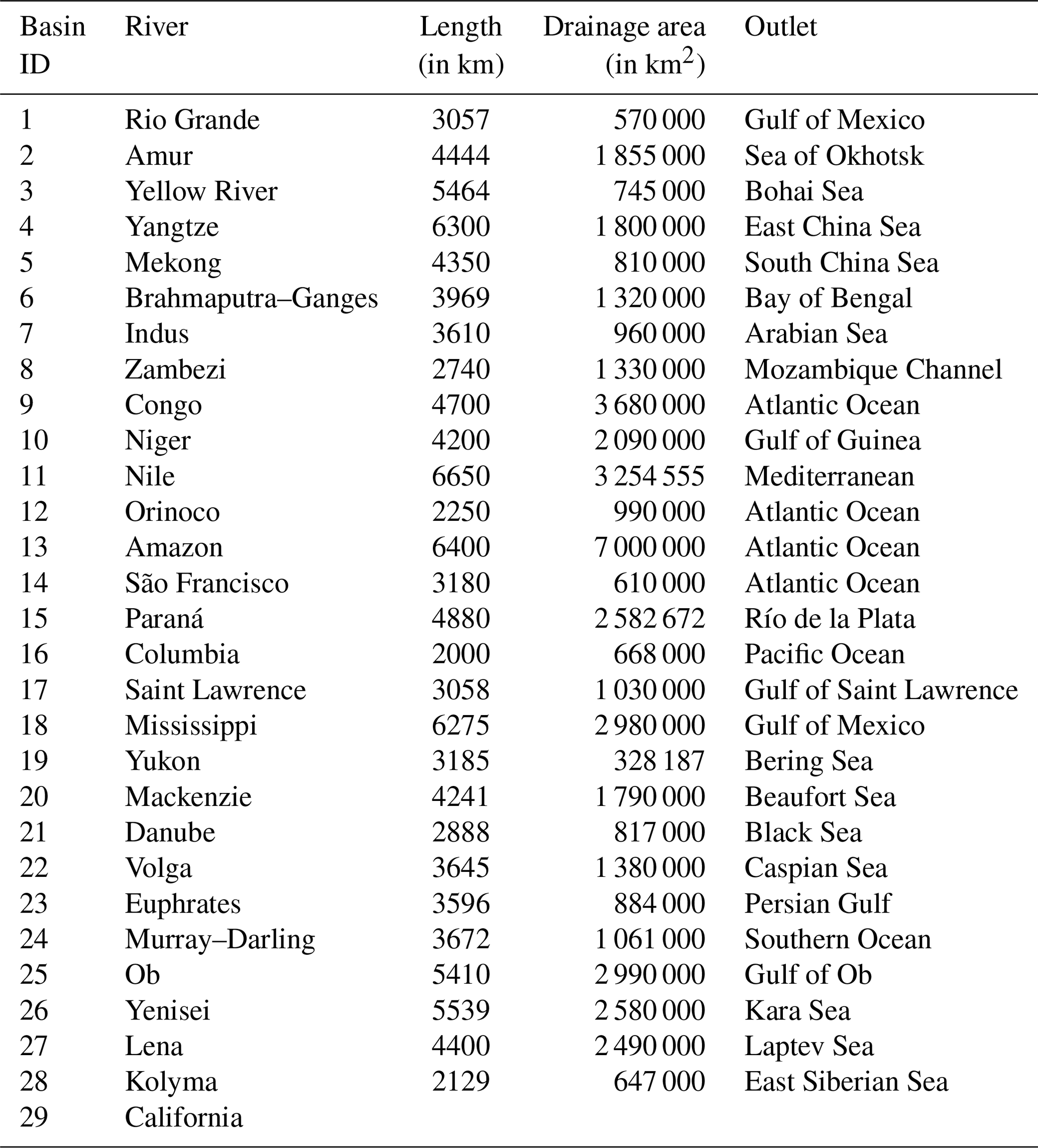
We selected 29 major global river basins (Fig. S1 in the Supplement) with drainage areas of ≥500 000 km2 (Table 1). According to the Köppen–Geiger climate (KGClim) classification scheme for 1984–2013 (Cui et al., 2021) (Fig. S2), these basins cover five climate zones: polar, boreal, temperate, arid, and tropical. In this study, we focused on boreal, temperate, arid, and tropical zones. The dataset referred to as KGClim is publicly available at 1 km spatial resolution and can be downloaded at https://doi.org/10.5281/zenodo.5347837 (Cui et al., 2021).
Table 1Summary of the length, drainage area, and outlet of the selected river basins.
2.2 GRACE data
We used release 6 (RL06) mascon solutions from the University of Texas Center for Space Research (CSR-M) and the Jet Propulsion Laboratory (JPL-M) water storage data (2003–2014) of equivalent water thickness. The data over the study period were sufficient to accommodate the average changes in the seasonal cycle of land water storage. Mascon solutions are great improvements over traditional spherical harmonics. Unlike spherical harmonics, mascon solutions do not require a postprocessing filter (Watkins et al., 2015; Save et al., 2016) and are more applicable to regional and global scales. JPL-M applies a coastline filter to attenuate the leakage between the ocean and land, and scale factors were applied at a grid scale to strengthen the signal smaller than 3 °. The CSR-M uses a finer hexagonal at a quarter-grid degree for coastline filters. The missing months in the GRACE record were filled using linear interpolation (Xiao et al., 2015; Liesch and Ohmer, 2016) as it is computationally efficient and straightforward to implement and preserves linear trends in the data. We used TWSC anomalies from JPL-M and CSR-M solutions in our study as these two solutions are widely recognized and have been extensively validated in the literature (i.e., Schellekens et al., 2017; Scanlon et al., 2021).
GRACE data can be accessed through these websites:
-
https://podaac.jpl.nasa.gov/dataset/TELLUS_GRACE_MASCON_CRI_GRID_RL06_V1 (last access: 20 January 2022)
-
http://www2.csr.utexas.edu/grace/RL06_mascons.html (last access: 11 February 2022).
2.3 EartH2Observe global water resource reanalysis data
We evaluated 13 hydrological models based on the global Water Resource Reanalysis (WRR). R1 and R2 models are Water Resource Reanalysis tier-1 and tier-2 products, which provide a large set of LSMs and GHMs developed by the eartH2Observe (E2O) (Schellekens et al., 2017). The model runs generated from WRR1 are abbreviated as R1, whereas model runs from WRR2 are abbreviated as R2. R1 is a 0.5° meteorological reanalysis dataset forced with ERA-Interim data (WFDEI) (1979 to 2012) (Weedon et al., 2014). R2 features a 0.25° meteorological reanalysis dataset forced with Multi-Source Weighted Ensemble Precipitation (MSWEP) data (1980 to 2014) (Beck et al., 2017). In R2 models, model algorithms were improved to better represent the hydrological processes by integrating anthropogenic impacts and Earth observation inclusions (Gründemann et al., 2018). A detailed description of these datasets and the improvement from R1 to R2 models can be found in Dutra et al. (2015, 2017) and Schellekens et al. (2017), respectively. The models used in this study are presented in Table S1 in the Supplement.
We investigated seasonal TWS anomalies from large-scale GHMs – including PCR-GLOBWB (R1 and R2), LISFLOOD (R1 and R2), HBV-SIMREG_R1, W3RA_R1, SWABM_R1, and WaterGAP3 (R1 and R2) – and LSMs – HTESSEL (R1 and R2), JULES_R1, and Surfex-Trip (R1 and R2).
To benchmark the selected models against GRACE TWSC (average JPL and CSR mascon), the 2003 to 2012 period was used as a common period for R1 and GRACE, and the 2003 to 2014 period was used for R2 models and GRACE TWS. E2O data can be accessed through the E2O Water Cycle Integrator portal (https://wci.earth2observe.eu/, last access: 10 March 2022).
2.4 Assessment of model performance
The monthly total water storage anomaly (TWSA) is the sum of all continental storage anomalies:
where SWSA is the surface water storage anomaly, SMSA is the soil moisture storage anomaly, GWSA is the groundwater storage anomaly, SnWA is the snow water equivalent anomaly, and CnWSA is the canopy water storage anomaly.
To derive the rate of change from the models, we used Eq. (2):
where TWSC is the climatological change in TWS; Q is the total outflow (net surface and groundwater outflow); t is time; and P and E are totals of precipitation and actual evapotranspiration, respectively.
The seasonal cycle was calculated by taking an average of each month (from January to December).
2.5 Statistical analysis
A Taylor diagram is a visual approach used to describe how well data (or datasets) correspond to the observations (Taylor, 2001). The resemblance between the two datasets was quantified using their correlation, cantered root-mean-square difference, and standard deviation. Taylor diagrams are particularly helpful in assessing various statistical aspects of complicated models or in evaluating the different models. Details of the correlation coefficient R and rms difference E are given in the Supplement.
We used the GRACE cycle to validate the GHMs' and LSMs' simulated seasonal cycles. We grouped models as GHMs (R1 and R2) and LSMs (R1 and R2) and presented the average behavior of each group against GRACE TWSC.
3.1 Comparison of seasonal peaks and amplitude between GRACE and models
This section compares the seasonal peaks and amplitude of TWSC derived from GRACE and 13 GHMs and LSMs over 29 basins in four climate zones (boreal, temperate, arid, and tropical). The seasonal peaks and amplitudes of TWSC exhibit variations in response to latitude and the corresponding climate zones. Figures 1–4 show the seasonal cycle of TWSC computed from the 13 model simulations (surrounding line charts with dashed lines for average values of GHMs (R1 and R2) and LSMs (R1 and R2)) over 29 basins and climate zone classification (center). Tables 3 and 4 illustrate the average peak magnitude and amplitude derived from GRACE, LSMs (R1 and R2), and GHMs (R1 and R2).
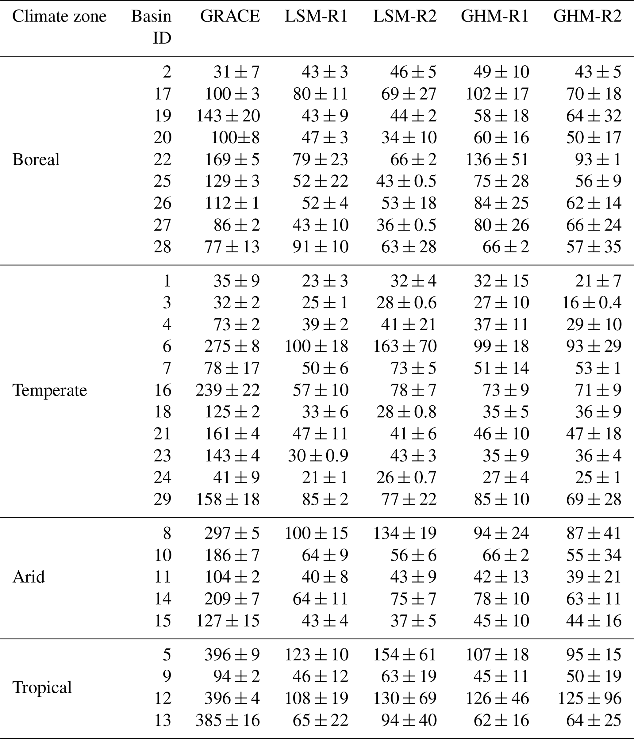
Figure 1 shows the seasonal variability of TWSC in the models and GRACE in snow-dominated catchments (boreal zone). GHM_R1 tends to overestimate the TWSC seasonal peak by ∼6–34 mm against GRACE in the boreal zone (with exceptions of the Mackenzie, Yukon, Ob, and Yenisei River basins, where the TWSC seasonal peak was underestimated by around 3–34 mm). GHM_R2 overestimated the peaks over Amur and Lena by ∼9 mm. For the mentioned basins, LSMs consistently underestimated TWSC peak magnitude by ∼6–49 mm (except for LSM_R2 being overestimated by ∼6 mm over Lena) (Table 3). In the Kolyma basin, the GRACE-observed seasonal peak measures 37±7 mm. GHMs performed well over this basin (they overestimated it by ∼2 mm), while LSMs (specifically R1) underestimated it by ∼15 mm. In the Yenisei and Ob basins, the GRACE-observed peak stands at ∼50–57 mm. Nevertheless, both LSMs and GHMs tend to underestimate TWSC, with LSMs falling short by about ∼25–31 mm and GHMs by approximately 7–20 mm for R1 and R2, respectively. In the boreal zone, the models' mean underestimated GRACE TWSC seasonal amplitudes by ∼2 %–69 % (Table 4), except over the Amur basin, where the models' mean TWSC was overestimated against GRACE by ∼38 %–58 %.
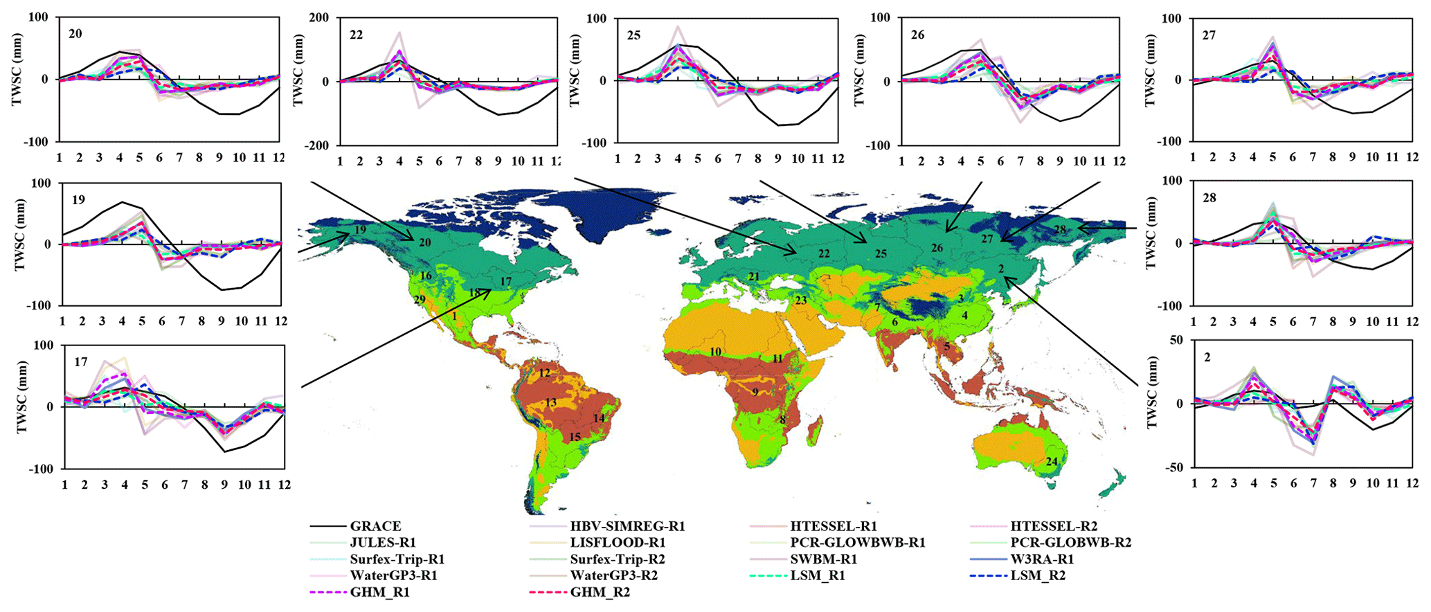
Figure 1Seasonal TWSC in the boreal zones from GRACE, GHMs, and LSMs. Base map represents KGClim climate zone classification. Details are provided in Fig. S2.
Over the temperate zone, all GHMs (R1) and LSMs (R1 and R2) underestimate the seasonal peaks by ∼7–112 mm (Fig. 2, Table 3). In Australia, the GRACE TWSC peak over the Murray–Darling River basin was recorded at 53±3 mm, and both LSMs and GHMs underestimated it by ∼40 mm.
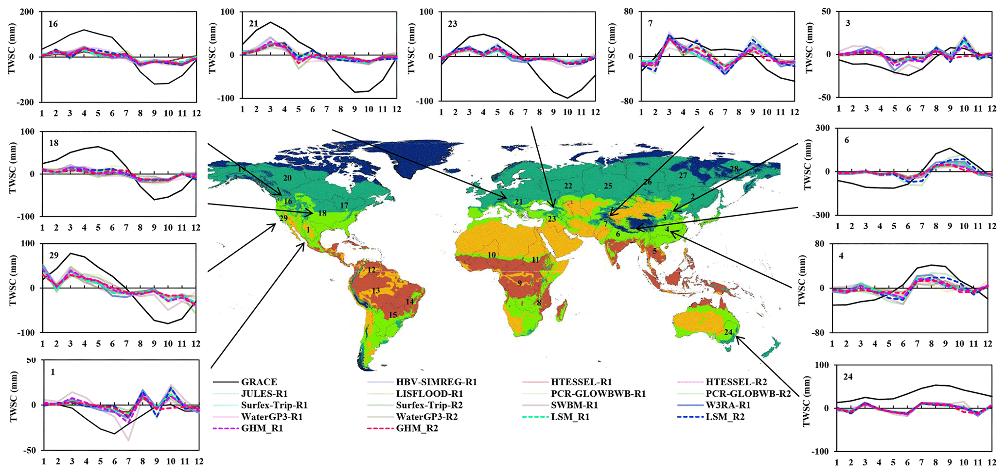
Figure 2Seasonal TWSC in the temperate zones from GRACE, GHMs, and LSMs. Base map represents KGClim climate zone classification. Details are provided in Fig. S2.
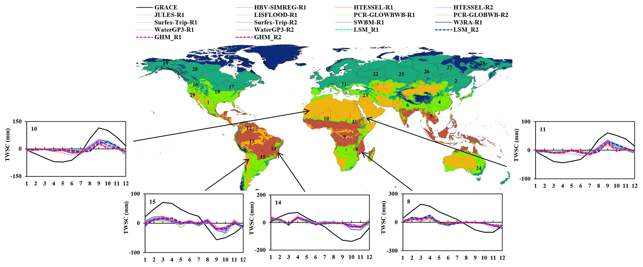
Figure 3Seasonal TWSC in the arid zones from GRACE, GHMs, and LSMs. Base map represents KGClim climate zone classification. Details are provided in Fig. S2.
Amongst Asian basins, the GRACE seasonal peak reached 42 mm over the Yangtze River basin. However, the average estimates from GHMs and LSMs fell short by ∼23–28 mm. The Yellow River basin exhibited weak GRACE signals, with TWSC peaks appearing at 8±1 mm; LSMs and GHM_R1 overestimated it by ∼2–9 mm, while GHM_R2 underestimated by ∼3 mm. Over two major river basins in Southeast Asia, the GRACE had strong signals in the Brahmaputra–Ganges River basin, where the TWSC peak was at 161±5 mm, while mean LSMs underestimated it by ∼72–105 mm, and GHMs underestimated it by ∼112 mm (Table 3). On the other hand, in the Indus River basin, GRACE signals were weak, and TWSC peaks appeared at 34±4 mm. LSM_R1 marginally underestimated the TWSC by ∼6 mm, while the LSM_R2 and GHM means underestimated it by ∼4 mm. In western Asia, the GRACE TWSC peak over the Euphrates basin was at 50±4 mm, whereas model means underestimated it by ∼29–38 mm. Furthermore, the GRACE seasonal peak was recorded as 76±5 mm over the European river basin of the Danube, while model means underestimated it by ∼45–54 mm.
In North America, models did not exhibit a pronounced seasonal cycle of water storage change. At the Columbia and Mississippi River basins, seasonal TWS fluctuations are subject to seasonal evolution of the moisture convergence. Over the Columbia basin, the GRACE TWSC peak was at 120±9 mm, though the model's mean was underestimated by ∼92 mm for LSM_R1 and by ∼81 mm for other model means. Mean model peaks appeared to be nearly flat against the GRACE TWSC seasonal peak (65±2 mm) in the Mississippi River basin, and models underestimated it by ∼53–55 mm. In the California region, the GRACE maximum storage change was 78±3 mm, and models underestimated it by ∼35–51 mm. Over the Rio Grande basin, GRACE signals were very weak, the TWSC peak was at 3±4 mm, and GHMs mean overestimated it by ∼6 mm. On the other hand, LSMs overestimated the TWSC peak by ∼8–16 mm. All the model means underestimated TWSC amplitude against GRACE TWSC by 64 %–79 % and 34 %–75 % for LSMs and GHMs, respectively (Table 4).
In arid basins, all the GHMs and LSMs underestimated the TWSC peaks by ∼36 to 145 mm (Fig. 3, Table 3). Over the Niger River basin, GRACE peaks appeared at 115±4 mm, while models underestimated it by ∼73 to 81 mm. Similarly, GRACE TWSC was observed at 61±2 mm in the Nile River basin, while model peaks were ∼29–36 mm below GRACE TWSC. Likewise, in the Zambezi, GRACE TWSC seasonal maxima were recorded at 190±5 mm, while models substantially underestimated the peak storage change, and model peaks appeared ∼118–142 mm below the GRACE TWSC. GRACE TWSC showed a clear climatology over the São Francisco and Paraná basins, with seasonal TWSC peaks at 73±3 and 71±8 mm, respectively, while the models underestimated them by ∼34–41 and ∼52–54 mm, respectively, compared against the GRACE signals. The models' behaviors were very ambiguous in these basins, especially over the Paraná River basin. Model means (all GHMs and LSMs) underestimated seasonal TWSC amplitude against GRACE TWSC; the difference between models and GRACE TWSC amplitude ranges between 54.5 %–70.9 % (Table 4).
Over the four tropical basins (Fig. 4), all models underestimated the seasonal TWSC crusts compared against that of GRACE. In the Mekong River basin, GRACE signals were very strong, and the TWSC peak was at 227±5 mm, while the GHMs and LSMs greatly underestimated it, and model TWSC crests ranged between ∼131–198 mm below the GRACE signals. Over the Congo River basin, the GRACE storage peak was at 45±1 mm, and model simulations fell short by ∼11–23 mm. In the Orinoco and Amazon basins, the GRACE peaks were at 180±2 and 184±4 mm, respectively, while models greatly underestimated it by ∼114–158 mm. The highest difference between the model and GRACE amplitude was observed over the Amazon basin (75 % to 83 %) in the tropical zone, while over the Congo River basin, the difference in amplitude was ∼32 %–52 %.
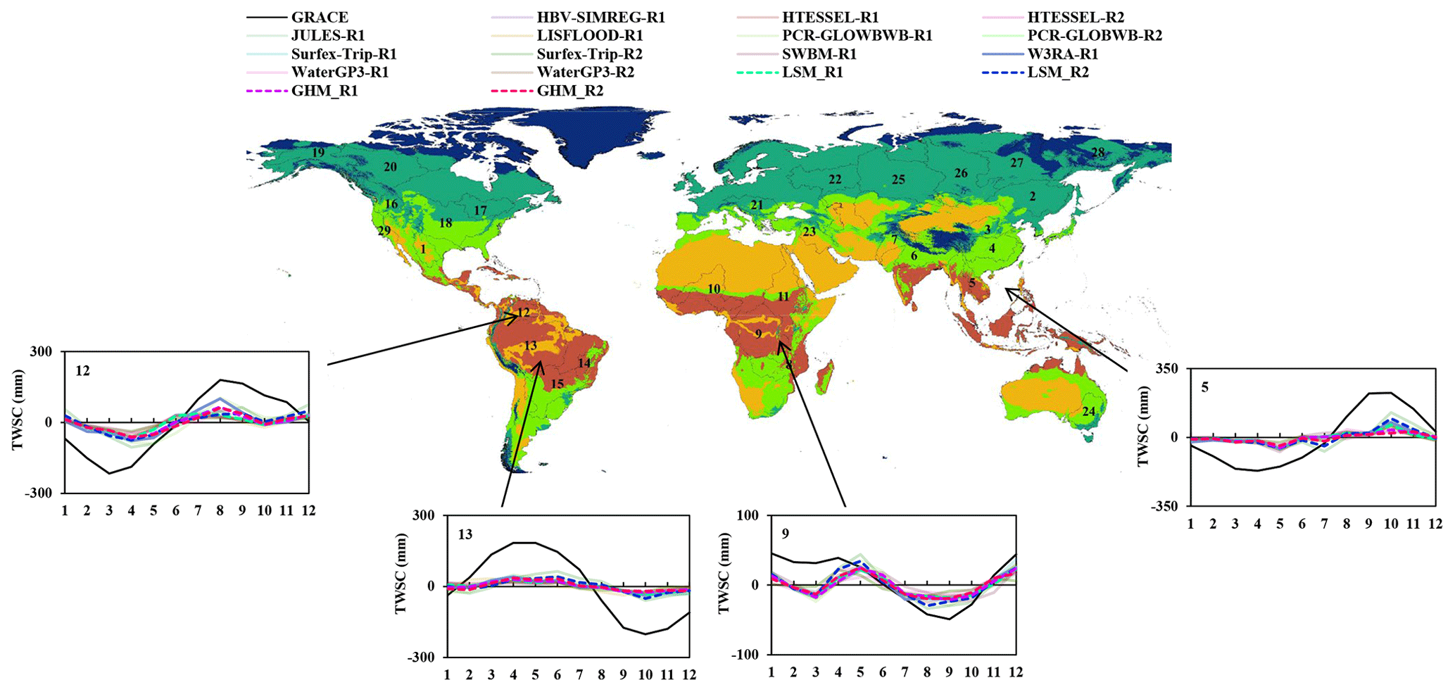
Figure 4Seasonal TWSC in the tropical zones from GRACE, GHMs, and LSMs. Base map represents KGClim climate zone classification. Details are provided in Fig. S2.
3.2 Phase difference between GRACE and models
The seasonal cycles of the boreal basins show TWS peaks in spring, which are largely generated by snowmelt. In snow-dominated basins (Fig. 1), seasonal TWSC variations from models and GRACE exhibited consistency in the timing of crest, except over the Saint Lawrence River basin, where R1 models peaks appeared 1 month earlier than GRACE, while troughs were inconsistent with GRACE TWSC over all the basins. The model TWSC precedes GRACE by 3–4 months. The trough in GRACE for all the basins started in September (except for the Kolyma and Amur basins, where they started in October), while in models, trough began in June, giving models a 3-month lead, except over the Yenisei and Amur basins (July) and Saint Lawrence (where most of the models showed ditch in May); models were 4 months ahead of GRACE observations. Figure 5 shows correlation coefficients of peak storage change at different time lags (months) between GRACE and model means. In Lena, LSM R1 showed the highest correlation with GRACE at a 1-month lag, indicating that peak storage in the R1 model occurred 1 month earlier than in GRACE.
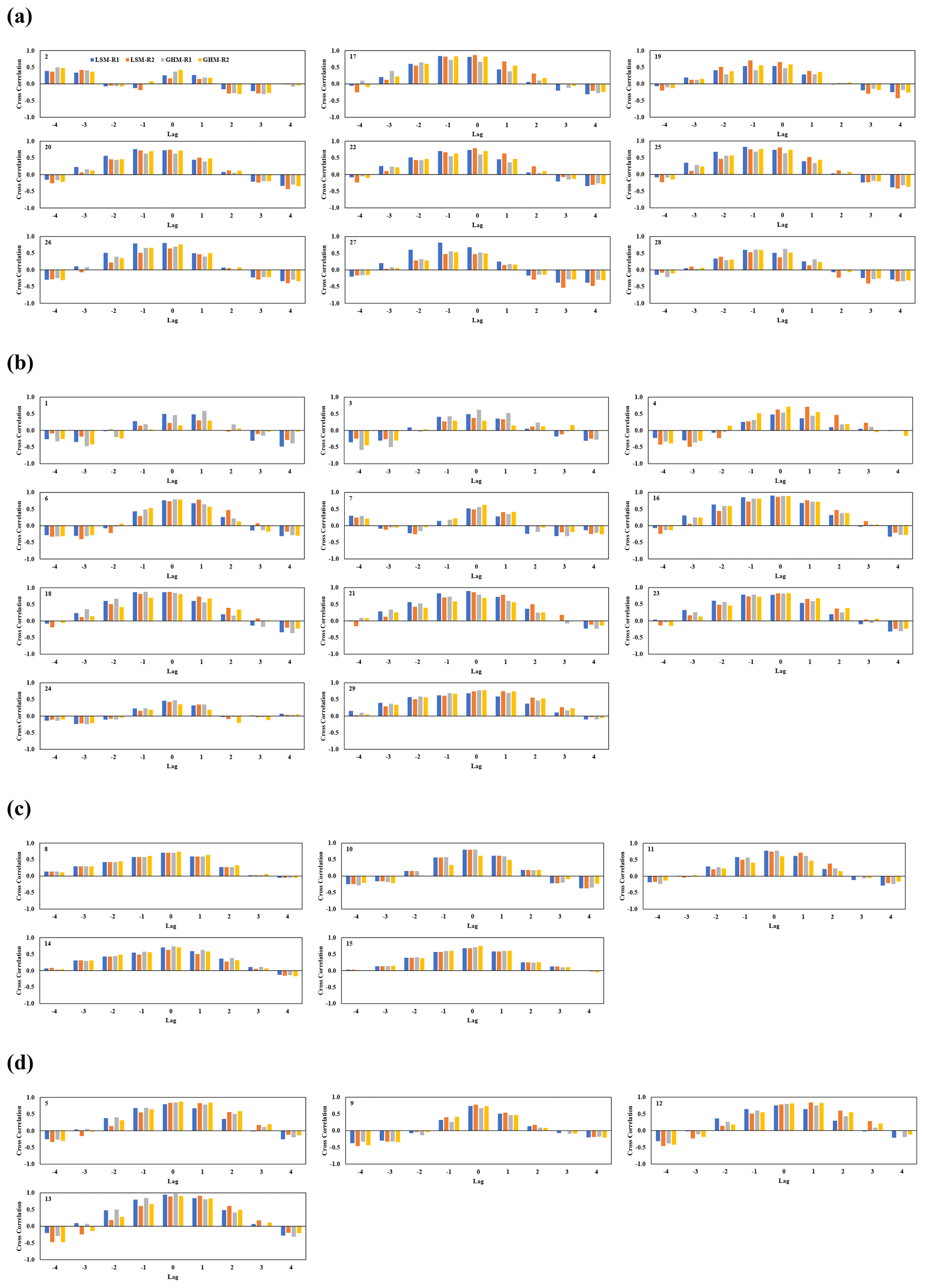
Figure 5The correlation coefficients at different time lags (months) between GRACE and the LSM (blue and orange bars for R1 and R2) and GHM (gray and yellow bars for R1 and R2, respectively). (a) Boreal, (b) temperate, (c) arid, and (d) tropical basins.
There was no phase difference between modeled and GRACE TWSC in the temperate zone, except for the Yellow River and Rio Grande River basin, where GRACE peaks were ahead of modeled TWSC by 1 month (Fig. 2).
In arid basins, modeled TWSC peaks have an identical phase compared to GRACE TWSC over the Niger and Nile River basins, while over the Zambezi and São Francisco River basins, modeled TWSC peaks appeared in April, resulting in a 1-month time lag over these two basins compared to GRACE, where peak storage was recorded in March (Fig. 3).
The model TWSC phases were quite consistent with GRACE over the Orinoco and Amazon River basins in the tropical zone. However, the GRACE peak over the Congo River basin was observed earlier in April, while modeled peaks were noted in May. Similarly, over the Mekong River, GRACE-observed peak water storage change was observed in September, while the models' peaks appeared in October (Fig. 4). Figure 5 shows the cross-correlation and time lag of LSMs and GHMs against GRACE over different basins in four climatic zones.
3.3 Evaluation of model performance
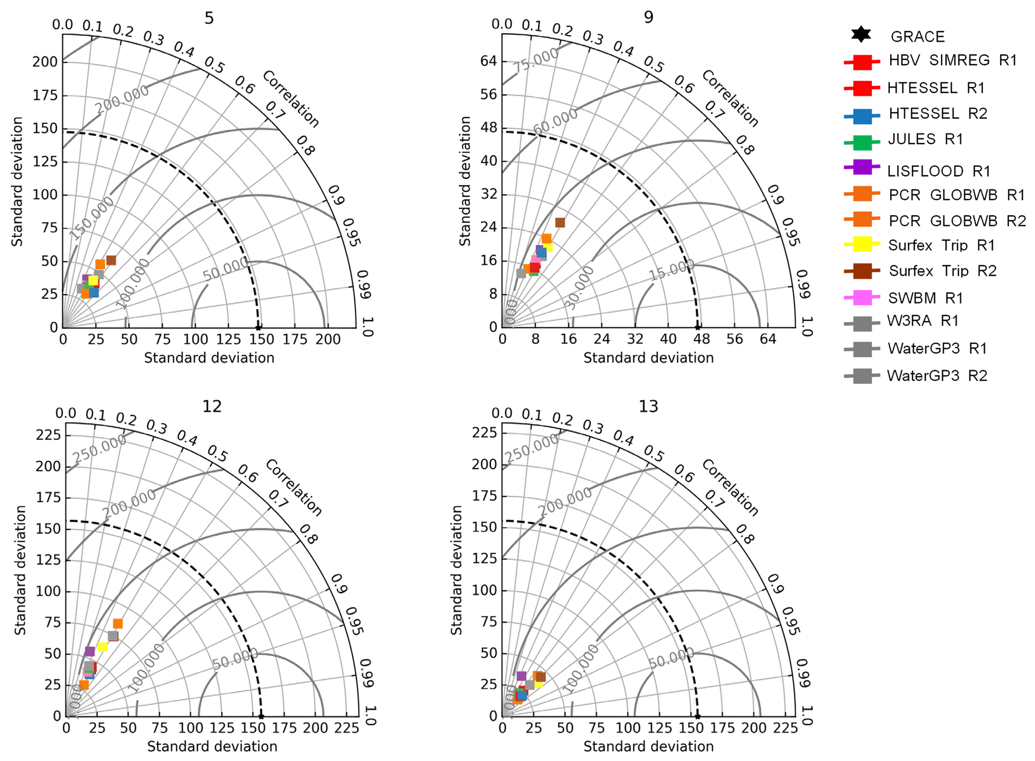
In cold basins (Fig. 6), the Taylor diagram does not clearly distinguish which of the 13 models better represents TWSC compared to GRACE. It is worth noting that correlations between the models and GRACE are weak over all the basins and range from R=0.1 to 0.5. The highest correlation (R=0.5) is found for the PCR-GLOBWB_R1, HTESSEL_R1, and HTESSEL_R2 over the Mackenzie, Volga, Ob, and Yenisei River basins, respectively. Almost all the models have smaller standard deviations than those observed by GRACE, while RMSE was very high and ranged between 25 to 90 mm.
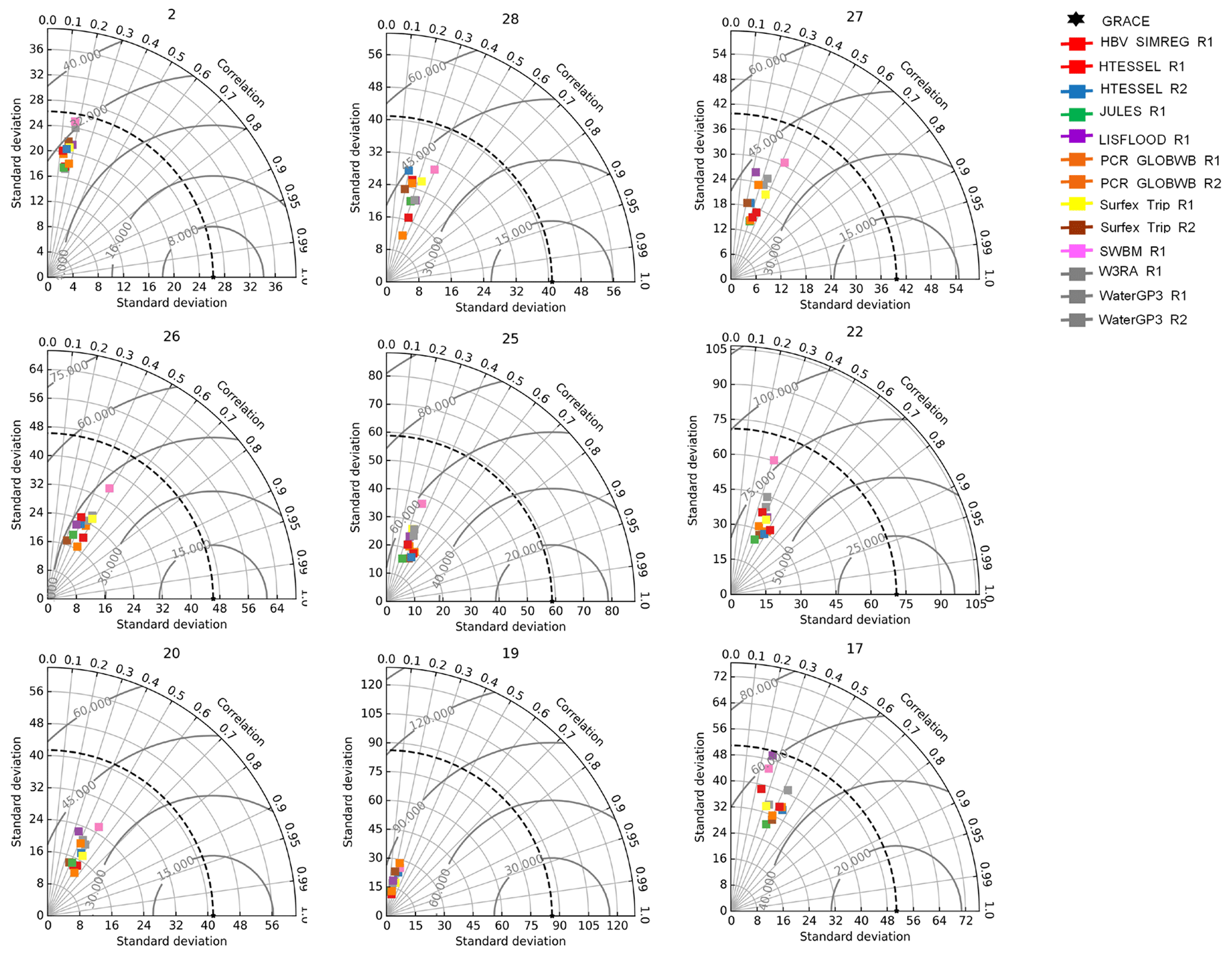
Figure 7 demonstrates the correlation between modeled and GRACE TWS over 11 temperate river basins. All 13 models had a good correlation with GRACE over the Columbia (R∼0.6) and Brahmaputra–Ganges River basins (R∼0.5 to 0.6) (except LISFLOOD_R1, SWBM_R1, and WaterGAP3_R1, which had a poor correlation over the Brahmaputra–Ganges River basin). Overall, SWBM_R1 demonstrated a good agreement with GRACE over the Euphrates, Columbia, and California, basins while LISFLOOD_R1 showed the lowest correlation against GRACE over this region., All the models exhibited no correlation with GRACE over the Rio Grande, Yellow River, and Yangtze River basins. All models have smaller standard deviations than GRACE observations, and RMSE ranged between 25 and 120 mm.
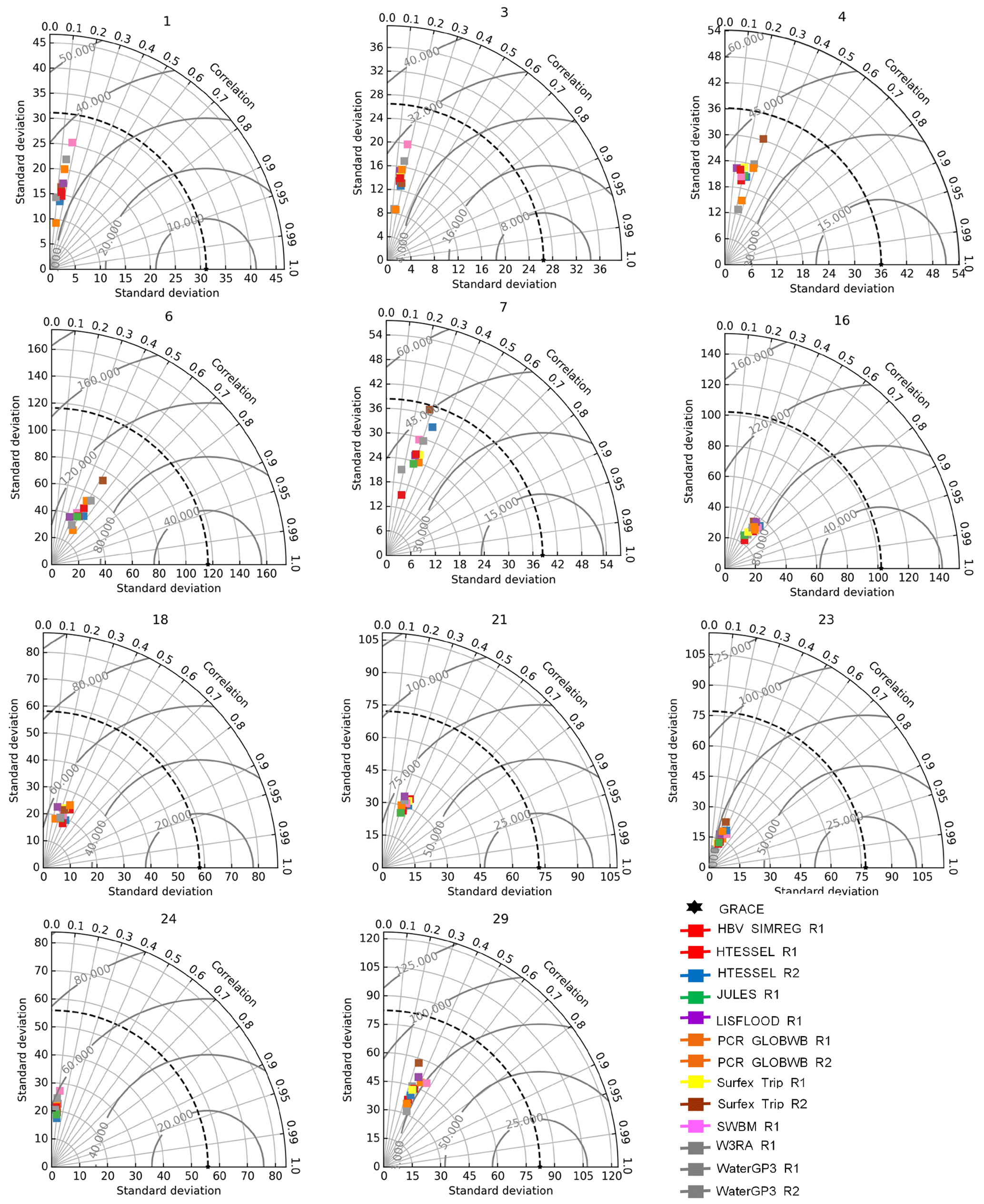
Figure 8 shows the correlation between models and GRACE TWSC climatology over five arid river basins. All 13 models had a strong correlation with GRACE over Niger River basins, with R ranging from 0.5 to 0.74. The highest correlation was observed for SWBM_R1 (r=0.74), and the lowest was observed for WaterGAP3_R1 (R=0.5). Furthermore, from the eight GHMs, HBV-SIMREG_R1, LISFLOOD_R1, PCR-GLOBWB_R1, SWBM_R1, and W3RA_R1 had good correlation over the Zambezi and Nile River basins, while all the five LSMs also showed good agreement with GRACE over the above-mentioned basins. All the models exhibited no correlation with GRACE over the São Francisco and Paraná River basins, except PCR-GLOBWB_R1, which had a good correlation with GRACE over the Paraná River basin. All models showed a lower standard deviation than GRACE over this region, and RMSE ranged between 30 and 110 mm.
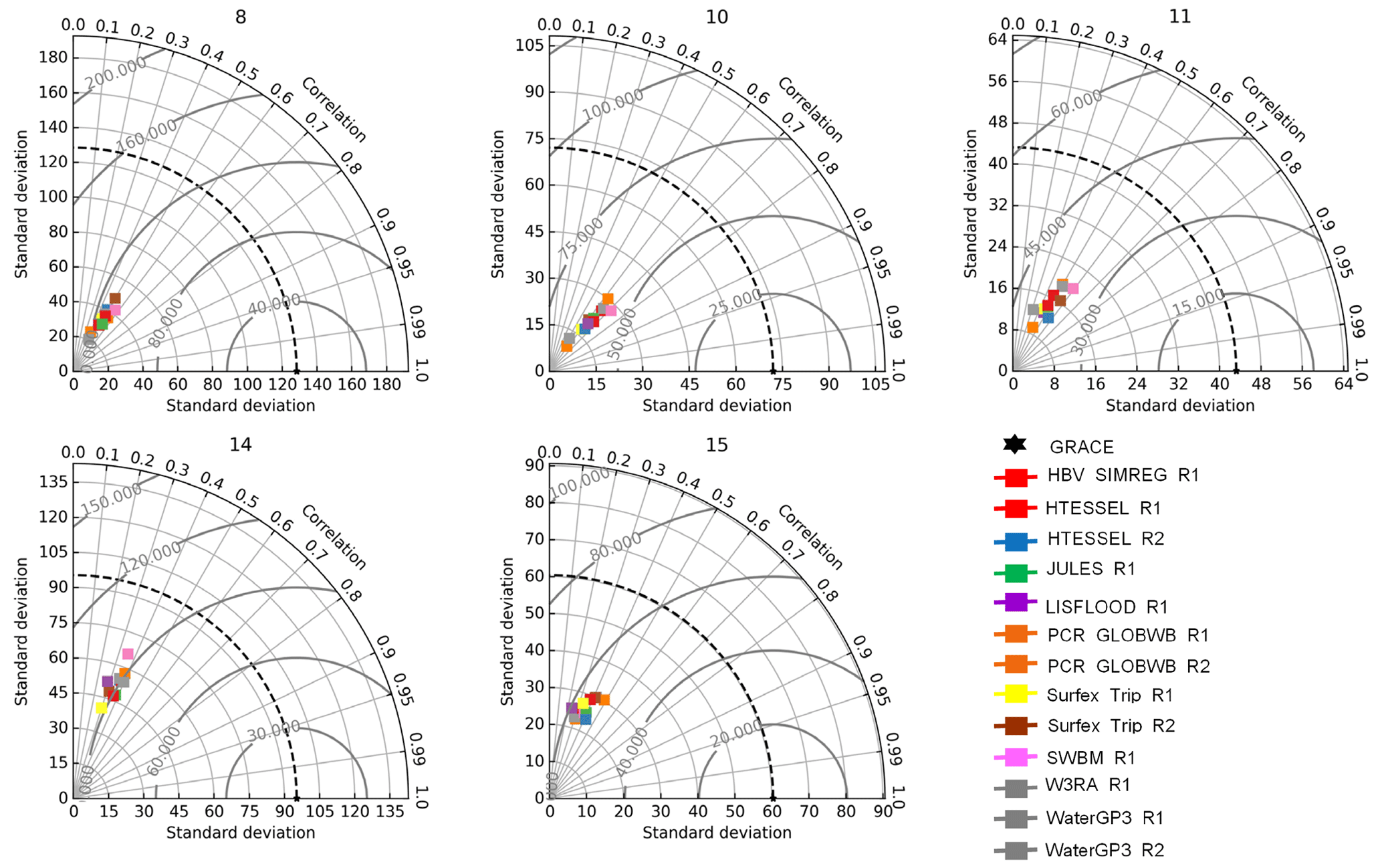
Figure 9 reveals that, compared to other climatic zones, models showed a good correlation with GRACE in the tropical zone. All models had a high correlation with GRACE over the Amazon River basins, with R=0.6–0.74, except LISFLOOD R1. Apart from HBV-SIMREG_R1 and W3RA_R1, other GHMs did not correlate with GRACE observations over the Congo River basin. Thus, HBV-SIMREG_R1 and W3RA_R1 were the best-performing models, while WaterGAP3_R1 was the least-performing GHM that correlated with GRACE only over the Amazon basin in this region. However, all LSMs exhibited excellent performance over these basins. Furthermore, R2 GHMs and LSMs revealed an excellent performance compared to R1 models. Almost all models have smaller standard deviations than GRACE-observed TWS, and RMSE ranged from 35 to 150 mm.
Figures 10 and 11 show the spatial relationship between the monthly time series of GRACE TWSC and the modeled TWSC (GHMs and LSMs, respectively). Figure 10 reveals a spatial correlation between the GRACE and GHM (R1 and R2) TWSC. Some models' TWSC, i.e., that of HBV_SIMREG_R1 and PCR_GLOBWB_R1, had a good correlation () with GRACE over some basins, i.e., the Amazon, Murray–Darling, and Indus River basins. For LSMs in Fig. 11, the R2 models showed a better correlation with GRACE TWSC than the R1 model. Two R2 models, HTESSE_R2 and Surfex-Trip_R2, showed a good correlation with GRACE over most of the basins. However, this correlation analysis did not illustrate any evident pattern of correlation (pixel correlation) at the basin scale between GRACE and LSM monthly time series (Fig. 11). Therefore, the seasonal analysis is a reasonable approach to access the model performance compared to GRACE-observed TWSC. Figures S3 and S4 compared seasonal maps of GRACE observations and TWSC estimated from GHMs and LSMs (FMA – spring, MJJ – summer, ASO – autumn, and NDJ – winter). The seasonal map in Figs. S5 and S6 revealed that the seasonal peak of GRACE is higher than GHMs and LSMs, except in the boreal zone.
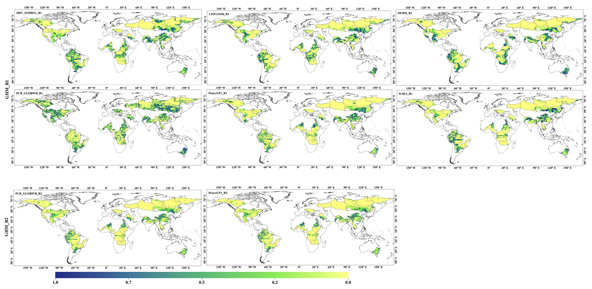
Figure 10Spatial correlation coefficient between GRACE and GHM (R1 and R2).
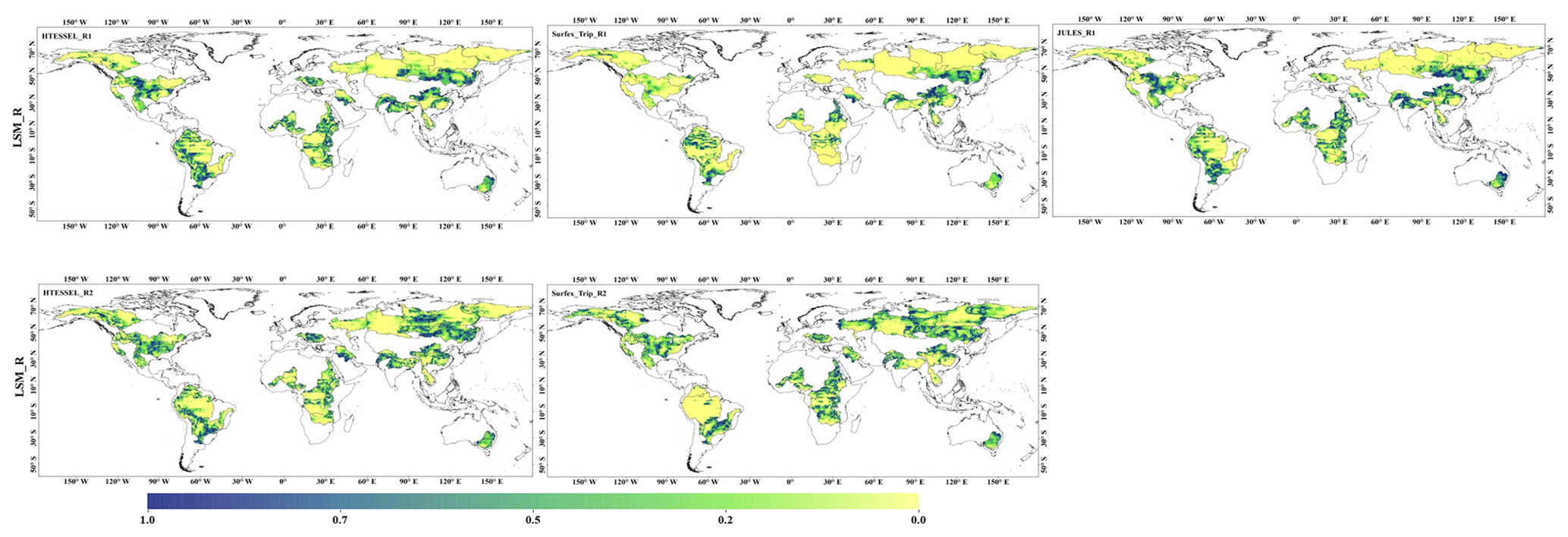
Figure 11Spatial correlation coefficient between GRACE and LSM (R1 and R2).
Across a range of timescales, seasonal features are more frequently used as analytical tools. Seasonal variations in TWS play a crucial role in understanding the water dynamics of a region, but they have received little attention due to a lack of independent data. We investigate multimodal seasonal TWSC considering peaks and phases from 13 models against GRACE. We first discussed the seasonal TWSC from GHMs and LSMs benchmarked against GRACE and identified disparities in their peaks and timing in different climatic zones. Table 5 summarizes the performance metrics of seasonal TWSC changes computed from 13 GHMs and LSMs against GRACE TWSC, where blue boxes corresponded to higher correlation and better performance, while red boxes indicated lower scores and poor representation. Overall, the model performed differently in the Northern Hemisphere (boreal zones), which is largely dominated by snow. When models simulate the climate patterns, they consider complex interactions between the atmosphere, land surface, and snow cover; snow modeling might be the most important factor in this region (Schellekens et al., 2017). However, accurately representing these processes in models can be challenging due to the inherent complexities of the climate system and the limited observational data available. As a result, model behavior in regions dominated by snow, such as boreal zones, may exhibit some discrepancies when compared to real-world observations.
In the Yukon and Mackenzie River basins in North America and in the Serbian basins, e.g., Lena, Yenisei, and Kolyma, water storage is mainly controlled by changes in snow cover. Models did not show good correlation performance, except for PCR-GLOBWB_R1 and HTESSEL (R1 and R2), which exhibited good correlation with GRACE over the basins located between 120° W to 100° E. R2 GHMs (PCR-GLOBWB_R2) and LSMs (HTESSEL_R2 and Surfex-Trip_R2) showed much poorer performance than the R1 models. Differences in simulations can be ascribed to the models' structures and their internal dynamics (Bolaños Chavarría et al., 2022). The poor representation of HTESSEL_R2 and Surfex-Trip_R2 could be attributed to various factors, including inaccuracies in simulating snow processes, deficiencies in representing other hydrological processes, and inadequate model calibration and/or validation. There is also the matter of model complexity – e.g., with an increased number of soil layers in HTESSEL_R2 (Table S2), one needs to account for additional vertical variations in soil properties, such as moisture content, temperature, and hydraulic conductivity. This complexity introduces more parameters and requires more accurate input data for each layer. If the additional layers are not properly calibrated or if the required input data are not available, it can result in increased uncertainty and poorer model performance. Similarly, Surfex-Trip_R2 has improved groundwater, surface energy and snow, flood plains, plant growth, and land use compared to the R1 model. However, if the improvements are not properly accounted for, if the model does not accurately simulate the interactions between plant growth and other hydrological processes, or if the improved vegetation parameters are not properly calibrated, they can introduce biases or inaccuracies that adversely affect the model's performance. Furthermore, improvements in R2 models generally influence reservoir storage rather than surface fluxes (Emanuel et al., 2017). Moreover, the poor performance of PCR-GLOBWB_R2 in the boreal region could be ascribed to a lack of a realistic depiction of the glacier and ice dynamics (Sutanudjaja et al., 2018). Improving the representation of glacier and ice dynamics in PCR-GLOBWB_R2 would require enhancements in the model's parameterization schemes and input data. This could involve incorporating more detailed information on glacier geometry, ice thickness, and movement patterns using remote sensing data, ground-based observations, and specialized glacier models. Additionally, considering the interactions between glaciers and climate variables, such as temperature, precipitation, and radiation, would be crucial for capturing the complex feedback mechanisms, or it may just be the presence of water storage in the cold basins that models fail to simulate accurately.
In the temperate regions, all GHMs demonstrated strong agreement with GRACE over the Columbia basin. Among the GHMs, HBV-SIMREG_R1, PCR-GLOBWB (R1 and R2), W3RA_R1, and WaterGAP3_R2 also showed good performance over the Brahmaputra–Ganges River basins. All the LSMs also showed excellent performance against GRACE over this basin, and HTESSEL_R2 had a good correlation with GRACE (R=0.62). Similar findings were reported by Zhang et al. (2017). Disparities between GRACE and models over other temperate basins can be attributed to the structure of the models, different water storage components for TWS calculation, different parameterization, and differences in runoff simulation and evaporation schemes (Zhang et al., 2017). In our case, the best-performing models are HBV-SIMREG_R1, W3RA_R1, JULES, HTESSEL (R1, R2), and Surfex-Trip (R1 and R2), which calculated the runoff by saturation and infiltration excess and used the Penman–Monteith method for evapotranspiration (Table 2). Nevertheless, the LISFLOOD_R1 also used the same parameterization scheme. PCR-GLOBWB_R2 and SWBM_R1 also used a similar approach for runoff generation but a different method to calculate evapotranspiration (Hamon (tier 1) or imposed as forcing for PCR-GLOBWB and inferred from net radiation in SWBM), while in WaterGAP3, evapotranspiration was calculated by the Priestly–Taylor method, and the beta function was used for runoff calculation. To gain a more detailed understanding of why these models behave differently over different basins in the temperate regions, it would be necessary to conduct a comprehensive analysis that investigates the specific aspects mentioned above for each model and basin of interest. However, the R2 models' performances were comparatively better than the R1 models in the temperate zone. This is consistent with a previous study of the medium-sized basin in Columbia (Bolaños Chavarría et al., 2022).
Table 2Models overview and key changes from WRR1 to WRR2.
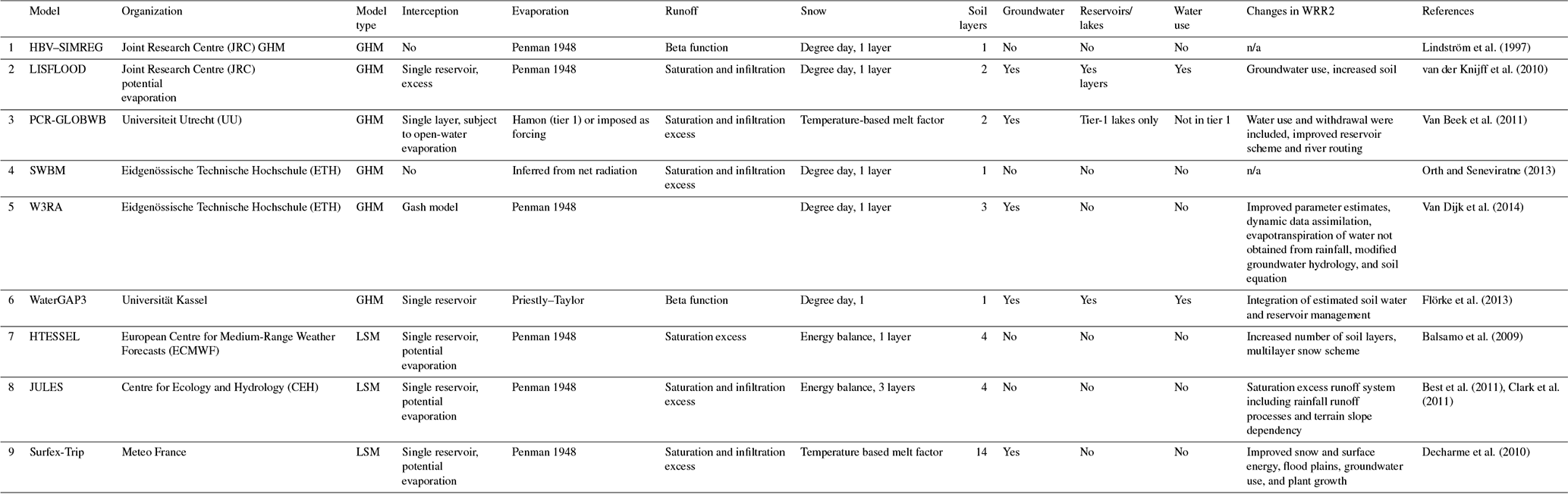
n/a stands for not applicable.
Table 3Peak magnitude (mm) derived from GRACE, LSM_R1, LSM_R2, GHM_R1, and GHM_R2; ± is the standard deviation.
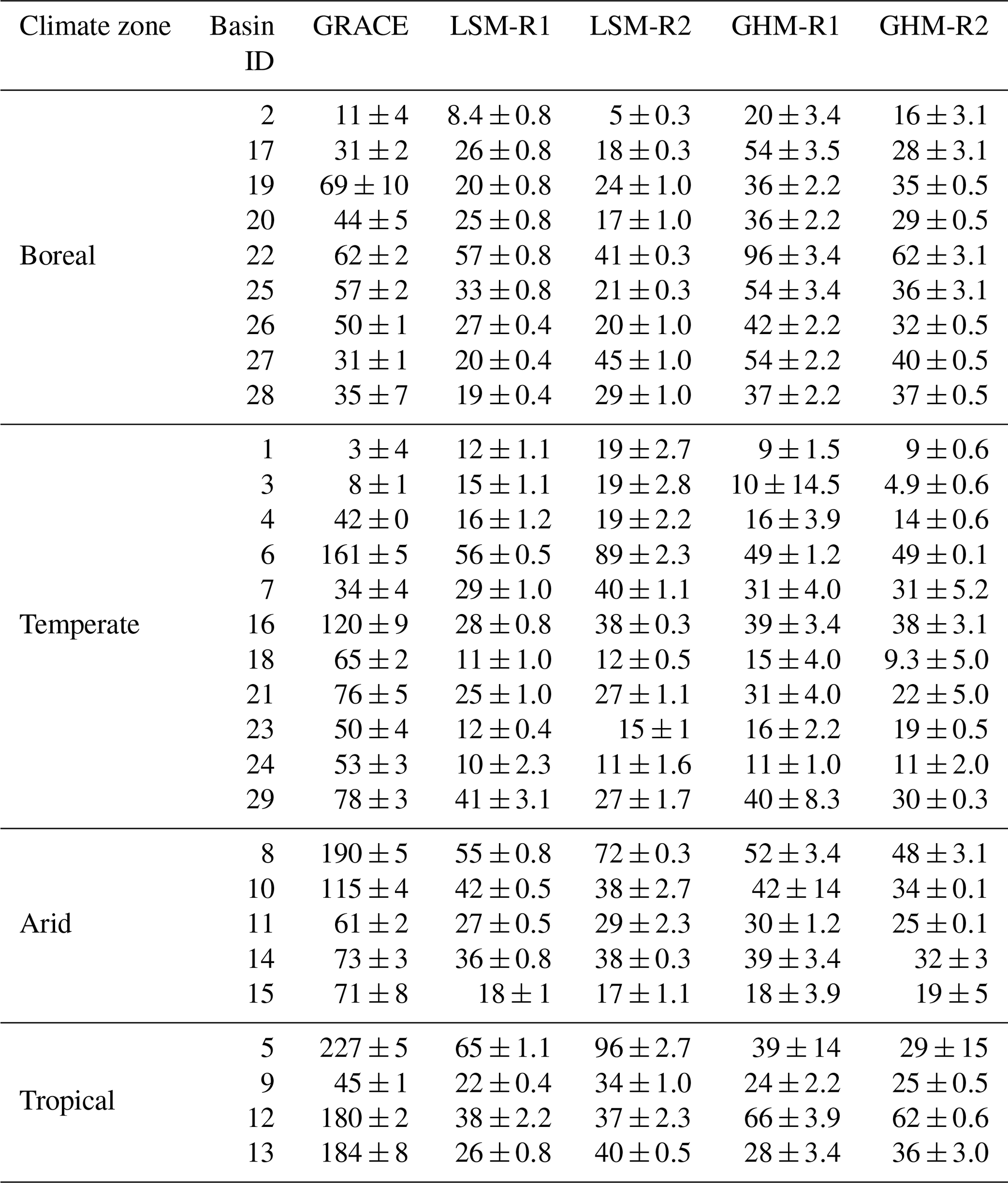
Table 4Amplitude (mm) derived from GRACE, LSM_R1, LSM_R2, GHM_R1, and GHM_R2; ± is the standard deviation.

In arid basins where subsurface water is the chief controller of TWSC variations, GHMs and LSMs exhibited a good correlation with GRACE observations over the Niger and Nile River basins. In the Niger River basin, the highest correlation was found for SWBM_R1, HBV-SIMREG_R1, and HTESSEL_R1. Furthermore, HBV-SIMREG_R1, LISFLOOD_R1, PCR-GLOBWB_R1, SWBM_R1, and W3RA_R1 had good correlation over Zambezi and Nile River basins, while all the LSMs also showed good agreement with GRACE over the above-mentioned basins. Our results are supported by a previous study conducted over the Niger and Nile River basins, where JSBACH and MPI-HM models exhibited a quite similar TWSC annual cycle when compared to GRACE (Zhang et al., 2017). However, the models behaved differently over different basins regardless of the differences in the models' structures. PCR-GLOBWB_R2 and WaterGAP3_R2 were among the least-performing models. However, in a previous study of the Limpopo River basin in southern Africa, WaterGAP3_R2 demonstrated the best performance in simulating flood events (Gründemann et al., 2018). The improved routing scheme in PCR-GLOBWB_R2, incorporation of water uses and groundwater abstraction, and reservoir management can also cause significant differences between the models because the addition of more sophisticated routing schemes and the incorporation of various water management components increase the complexity of the model. With added complexity, there is an inherent risk of introducing additional uncertainties or errors into the model. The interactions between different components and processes in the model can become more intricate, making it challenging to accurately capture TWSC. To incorporate water use, groundwater abstraction, and reservoir management components into PCR-GLOBWB_R2, certain assumptions and simplifications have been made. These assumptions can introduce biases or inaccuracies into the estimation.
Over the tropical regions, modeled TWSC had a strong correlation with GRACE observations in the Amazon basin in terms of phase, but models underestimated TWSC peaks. This indicates that the models were able to simulate the seasonal and interannual fluctuations in water storage, aligning with the observed patterns. However, the fact that the models underestimated the peaks of TWSC indicates that they did not accurately reproduce the magnitudes of water storage changes as observed by GRACE. Among other models, HBV-SIMREG_R1, PCR-GLOBWB (R1 and R2), W3RA_R1, WaterGAP3 (R1 and R2), HTESSEL_R2, and Surfex-Trip (R1 and R2) demonstrated an excellent representation of TWSC in the Amazon basin, where river channel storage is the most important factor in the seasonal TWSC variations, and accurate representation of the dynamics in hydrological models is crucial. This includes accounting for river routing, floodplain dynamics, and water exchanges between the river channels and other storage components. LISFLOOD_R1 did not show any correlation with GRACE over any of the five tropical basins, and our results are supported by similar findings reported in a previous study where LISFLOOD_R1 was the worst-performing model over medium tropical basins (Bolaños Chavarría et al., 2022). Similar findings were reported in a previous study (Scanlon et al., 2019) where the model underestimated seasonal TWSC in the subtropical zone ° near the Equator, where modeled medians were up to ∼40 % less than GRACE. LISFLOOD simulates surface water dynamics, including river flow, floodplains, and surface water storage. However, the model might have inherent limitations or simplifications that affect its ability to capture the complex hydrological processes specific to the tropical basins. The model's representation of important factors such as vegetation dynamics, groundwater interactions, or human activities might be inadequate for these regions.
Furthermore, the prevailing pattern may indicate that it is associated with subsided model performance in heavily regulated channel reaches and simulation of man-made structures; i.e., reservoirs remain challenging in the LISFLOOD model (van der Knijff et al., 2010). Overall, the R2 (PCR-GLOBWB_R2, WaterGAP3_R2, HTESSEL_R2, and Surfex-Trip_R2) models showed greater agreement with GRACE than the R1 models. Figures S5–S8 exhibit the distribution of GRACE and grouped model type (GHM or LSM) and forcing resolution (R1 and R2) in four climate zones. Disparities in the seasonal signal of TWSC between GRACE and the models can be caused by uncertainties in the models, in GRACE, or in both (Scanlon et al., 2019). Zhang et al. (2017) used GRACE observations to validate TWSC simulations from four numerical models over 31 global river basins. They observed that, over most of the basins, GRACE error was much smaller than RMS differences, and they concluded that model uncertainties were the primary cause of the differences. These biases can also result from the simulated storage capacity and storage compartments, e.g., SW and GW in the model; uncertainties in inflow or outflow runoff generation; and human intervention in the case of GHM or its absence in the case of LSM.
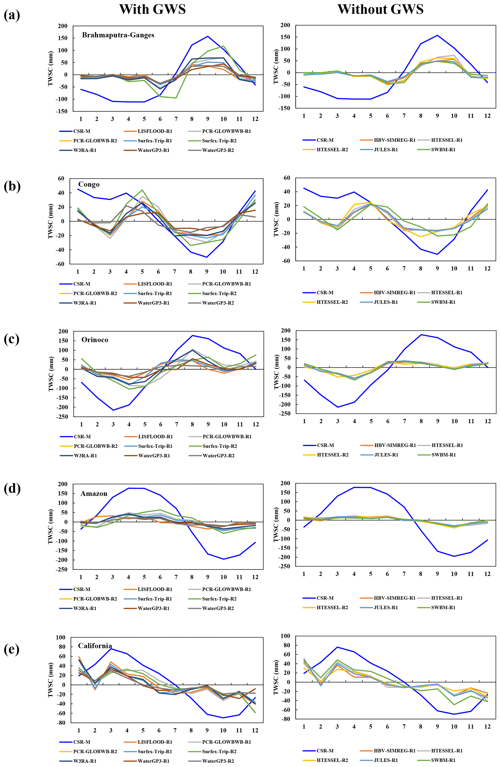
Figure 12Comparison between seasonal TWSC from GRACE and models with and without groundwater simulations in (a) Ganges–Brahmaputra, (b) Congo, (c) Orinoco, (d) Amazon, and (e) California basins.
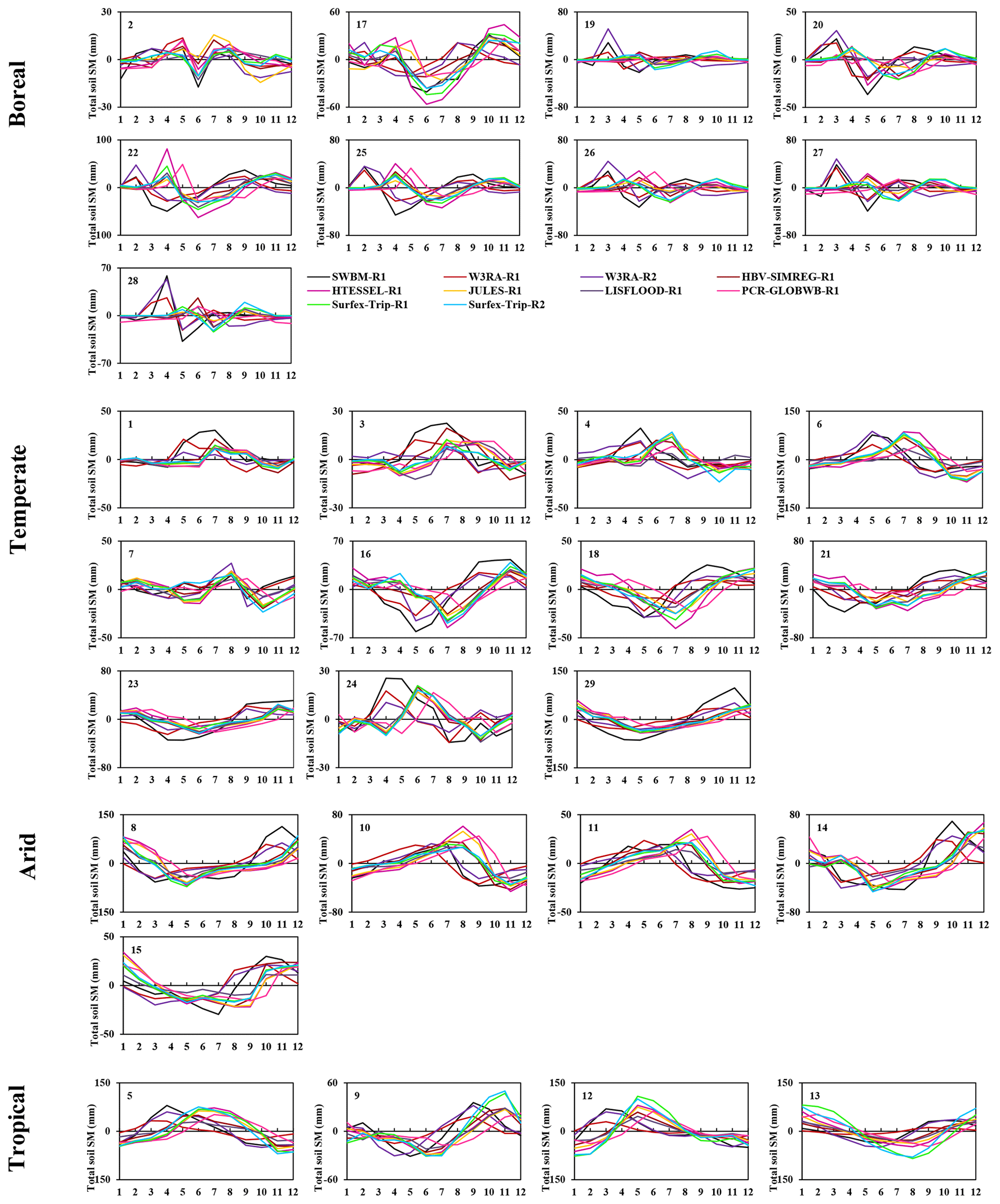
Figure 13Seasonal total soil moisture (SM) anomalies in the boreal, temperate, arid, and tropical zones in GHMs and LSMs.
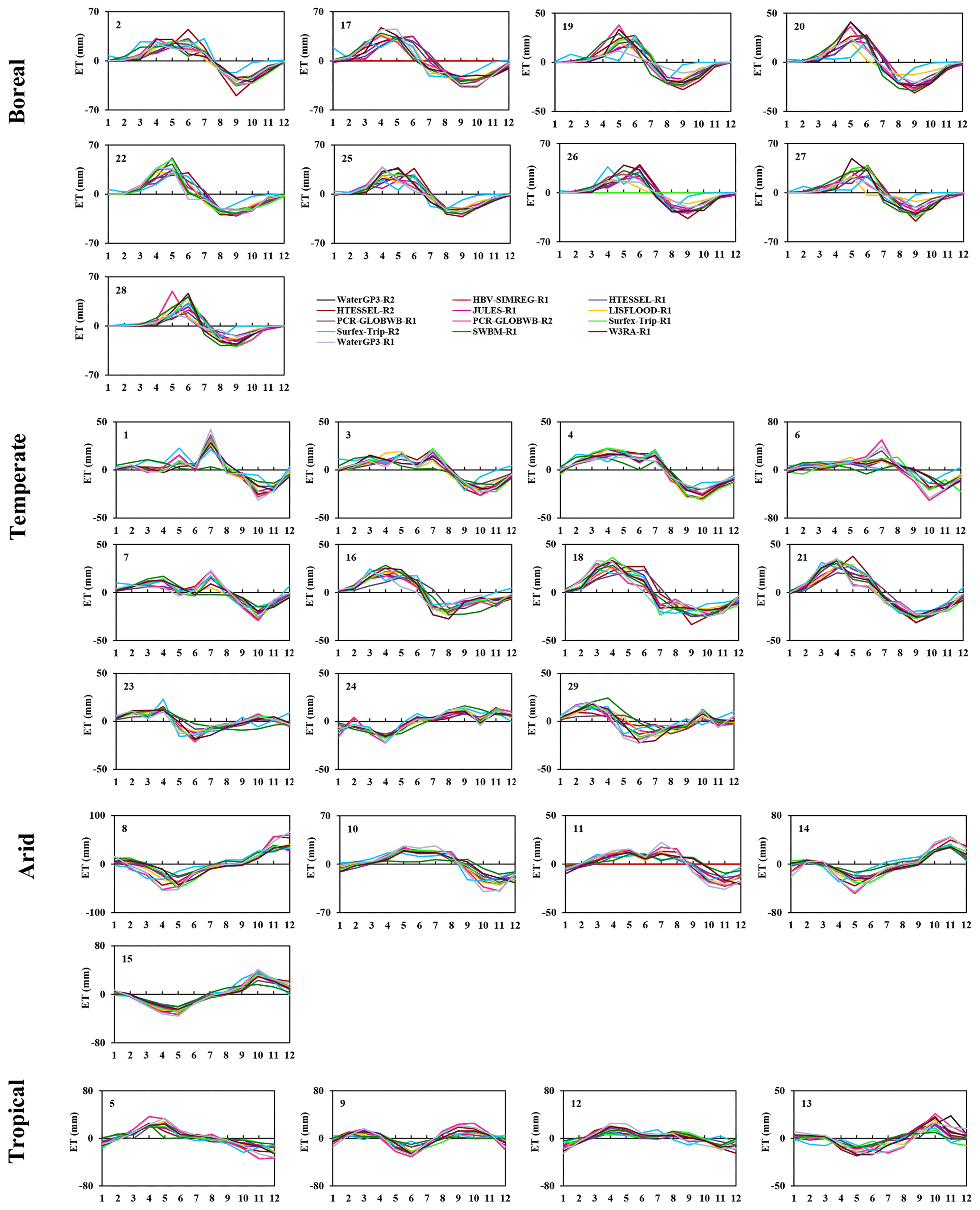
Figure 14Seasonal ET anomalies in the boreal, temperate, arid and tropical zones in GHMs and LSMs.
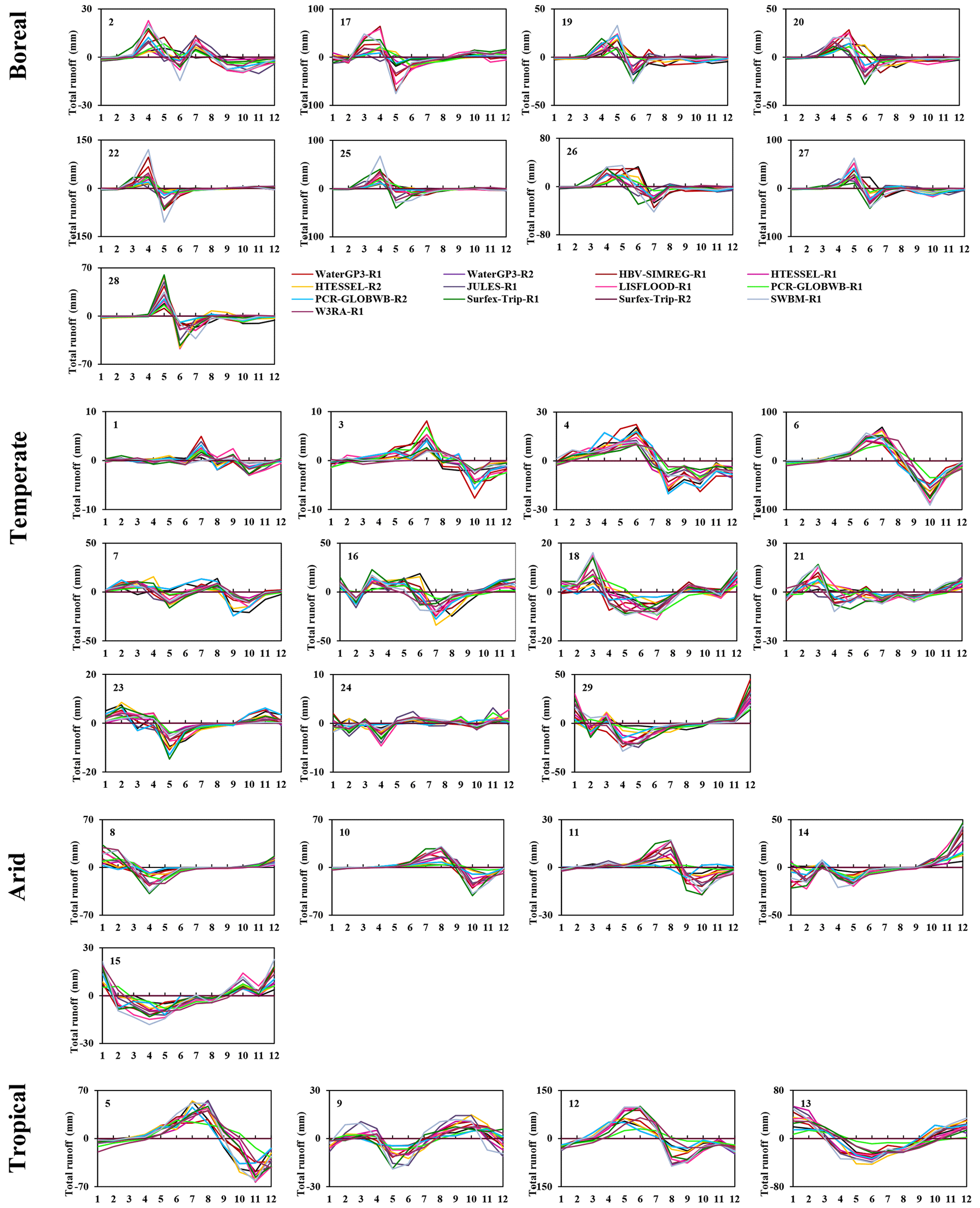
Figure 15Seasonal total runoff anomalies in the boreal, temperate, arid and tropical zones in GHMs and LSMs.
4.1 Causes of discrepancies in seasonal peaks and phases between models and GRACE TWSC
The differences in seasonal peaks and phases between GHMs and LSMs (R1 and R2) and GRACE TWSC can be attributed to several factors:
-
Model physics and assumptions. Each GHM and LSM utilizes a different set of equations, parameters, and assumptions to simulate the water cycle processes, including precipitation, evapotranspiration, groundwater flow, soil properties, vegetation dynamics, and runoff generation mechanisms (Table 2). These differences can lead to variations in how the models respond to the same input data. For instance, Fig. 12 shows a comparison between models with and without groundwater simulations over the Ganges–Brahmaputra, Congo, Orinoco, Amazon, and California basins with major underlying aquifers (https://www.un-igrac.org/resource/whymap-groundwater-resources-world-incl-thematic, last access: 15 July 2023). Over the Orinoco and Amazon basins, models without groundwater simulation greatly underestimated the seasonal water storage against GRACE observations; however, over the Ganges–Brahmaputra, Congo, and California basins, there was no big difference in seasonal TWSC amplitudes between models with and without groundwater, except for Surfex-Trip-R2 and PCR-GLOWBWB-R1 (only over Congo and California). Similarly, as shown in Fig. 1, there is a significant spread among the models (GHMs and LSMs) over cold regions, possibly due to different treatment of snow processes in each model. According to Schellekens et al. (2017), there is a discrepancy in the boreal zone's precipitation data, which may be another factor contributing to the wide variation between models and underestimation of TWSC compared to GRACE. Furthermore, models operate at coarse spatial resolutions, which may not capture the intricate details of the hydrological processes. For example, the models may not adequately simulate snowmelt, glacier dynamics, or the influence of local hydrogeological features that can affect water storage. In a region with small-scale land use changes or variations in soil properties, like urban development or agricultural practices, the model may not capture these variations adequately. This can result in peak differences between the model's output and GRACE observations. For instance, an improved parameterized model run of Surfex-Trip-R2 showed better agreement with GRACE TWSC over the Ganges–Brahmaputra, Congo, Orinoco, Amazon, and California basins (Fig. 12) compared to Surfex-Trip-R1.
-
Model parameterization. The overall structures of the model (like water storage compartment representation) and parameterization (like compartment capacity) play a critical role in model performance. The choice of soil properties and hydraulic conductivity parameters in the models significantly influences how water moves through the soil and contributes to runoff, groundwater recharge, and storage. Similarly, vegetation parameters, such as leaf area index (LAI), canopy resistance, and vegetation root depth, affect how much water is taken up by plants and transpired into the atmosphere. Most LSMs do not model SWS and GWS compartments, except for Surfex-Trip (Table 2). The partitioning of storage compartments like the soil layer also affects the model performance (Schellekens et al., 2017). As shown in Table 2, Surfex-Trip has 14 soil layers, while PCR-GLOWBWB-R1 has 2 layers, but both showed good agreement over the Congo and California basins; however, they did not agree well in many other basins. Furthermore, the thickness and total soil depth may be key factors in determining storage capacity in addition to the number of soil layers. According to Swenson and Lawrence (2015), an 8–10 m thick soil profile is needed to replicate GRACE TWSC in tropical basins such as the Amazon and Congo; however, the storage dynamics have been constrained as a majority of the models studied here have soil thicknesses between 1–4 m (Schellekens et al., 2017).
-
Inaccurate representation of human activities. Models that do not account for changes in land use and land cover, such as urbanization, deforestation, or agricultural expansion, may misrepresent the spatial distribution of surfaces and vegetation, affecting runoff and evapotranspiration patterns. Similarly, agriculture practices, such as irrigation, crop selection, and tillage practices, can significantly influence soil moisture dynamics and evapotranspiration rates. The presence and operation of reservoirs, dams, irrigation systems, and inter-basin water transfers can also alter river flow regimes, water storage, and groundwater recharge. Furthermore, water abstraction for domestic, industrial, and agricultural use besides irrigation can significantly impact water quantity. Inaccurate representation of these factors can lead to errors in simulating water balance components, including runoff, infiltration, and groundwater recharge. Table 2 shows that the majority of the models in the present study do not include reservoir or lake and water use modules, except for two GHMs, LISFLOOD and WaterGAP3. For PCR-GLOWBWB, the R1 model had lakes, but reservoirs and water use were not incorporated into it; in contrast, these components are incorporated into the R2 model (Schellekens et al., 2017). All these factors contributed indirectly to underestimations of TWSC against GRACE and discrepancies among the models.
-
Spatial resolution of input forcing data of the models. The data used to force the models were from the WFDEI and MSWEP datasets, with spatial resolutions of 0.5 and 0.25°, respectively, which are relatively coarse. These resolutions may not capture fine-scale variations in meteorological and environmental conditions within a grid cell. For models that require higher spatial detail to accurately represent local processes, using these datasets can lead to the loss of important information. Furthermore, the datasets assume uniform meteorological conditions within each 0.5 or 0.25° grid cell. In reality, conditions can vary significantly within a grid cell, especially in regions with complex topography or land cover changes. This can affect the representation of local hydrological processes (Trautmann et al., 2022). This could be another contributing factor for discrepancies among the models and underestimation of TWSC compared to GRACE over different regions (Figs. 1–4). Figure 13 shows seasonal total soil moisture (SM) anomalies of GHMs and LSMs in the four climate zones. There are large disparities in terms of SM anomalies amongst the models in various basins, even when the models are forced with the same input data, which directs the fact that the SM estimates have huge uncertainty, and further effort is required to enhance the outcomes.
-
Water fluxes. Models with the same climate forcing show a large spread in evapotranspiration (ET) seasonal amplitudes in different basins (Fig. 14). Even though this study does not specifically investigate variations in ET among the models, it is important to highlight that the wide array of methods employed by the models for calculating potential evapotranspiration (PET) could play a substantial role in the observed discrepancies. Schellekens et al. (2017) indicated that future updates to the dataset PET and net radiation calculation methods should be considered as these are likely major factors contributing to the observed variability in ET estimates. Similarly, in Fig. 15, the spread of total runoff derived from the GHMs and LSMs is fairly large. Different concepts of storage dynamics and runoff parameterizations, including the available energy partitioning, lead to a large spread among models for each basin. Schellekens et al. (2017) suggest that it is reasonable to consider the ensemble mean to be the most dependable estimate of global water fluxes, even though there is no independent method available to validate this assumption.
-
Uncertainty and errors in GRACE. GRACE measurements are affected by sources of error, such as atmospheric contamination and leakage effects (Scanlon et al., 2019). While GRACE satellite data provide valuable insights into TWSC, they also have limitations. The spatial resolution of GRACE data is relatively coarse, and the data are subject to errors and uncertainties. The GRACE satellite mission measures changes in Earth's gravity field, which can be transformed into estimates of changes in terrestrial water storage. Differences in data processing techniques, filtering, and corrections applied to GRACE data can lead to variations in the derived water storage estimates. Uncertainties and errors in models and GRACE observations can contribute to differences in seasonal peaks and phases.
It is important to note that the specific causes of differences can vary depending on the specific GHMs, LSMs, and GRACE products being compared. These are general possibilities, and the specific reasons for discrepancies may vary depending on the characteristics and complexities of each river basin and the model used.
4.2 Implications and outlook
Our multimodel seasonal TWSC comparison demonstrates the importance of using independent remote sensing data to evaluate GHMs and LSMs in diverse hydro-climatological settings. Our findings on seasonal assessments of peak storage change, amplitude, and phase difference provide future directions for model development, emphasizing the importance of an accurate representation of water stocks and other associated processes. It is important to note that models that include a more precise description of the internal storage dynamics provide a better comparison between simulated TWSC from global models and GRACE data. Comparing TWSC calculated from the balance of precipitation, evaporation, and observed basin outflow against directly computed TWSC variability from satellite observations may assist in finding models with improved structures and process representation.
This study evaluated 13 models (GHMs, LSMs) using different resolutions of the Water Resource Reanalysis (WRR1 and WRR2) to compare simulated total water storage change (TWSC) against GRACE observations over 29 major river basins. Model performance differs significantly across basins, even within the same climatic region. In snow-dominated basins, LSMs generally underestimate the TWSC peaks, and GHMs overestimate them. Models and GRACE exhibited consistency in the crust, but modeled TWSC preceded GRACE, with 3–4 months of lag in troughs. In temperate, arid, and tropical basins, GHMs and LSMs generally underestimate the peaks. However, the modeled TWSC phase is identical to that of GRACE, with a few exceptions. Furthermore, in basins with major underlying aquifers, models without groundwater simulation greatly underestimated the seasonal water storage changes compared against GRACE over the Orinoco and Amazon basins; however, over other basins with major underlying aquifers, there was no significant difference in seasonal TWSC amplitudes between models with and without groundwater modules.
For the Congo, Orinoco, and Ganges–Brahmaputra basins, those models incorporating groundwater simulations show substantially better agreement with GRACE and provide a more accurate depiction of the seasonal TWSC compared to the models without groundwater simulations.
Apart from uncertainties associated with GRACE measurements, it provides an independent means for model assessment. The negative phase differences between models and GRACE might indicate an overall underestimation of the TWS component (e.g., groundwater), leading to an overly rapid system response. The disparity in peaks and phases could suggest that either models are lacking stores, e.g., lakes and rivers, or the size of the stores is insufficient. There is no single model that performs best in all regions. However, performance statistics reveal that R2 models had a better correlation with GRACE than the coarse-resolution R1 models. This demonstrates that optimized model structure can increase the models' ability to simulate TWS variability and replicate water storage observations. Seasonal TWS variations have received little attention due to a lack of independent data for evaluation. The study provides insight into the peaks and phase differences between models and GRACE TWSC, which can potentially contribute to further improvement of GHMs and LSMs in the future.
GRACE data used in this study can be accessed through these websites: https://doi.org/10.5067/TEMSC-3MJC6 (NASA, 2024) and http://www2.csr.utexas.edu/grace/RL06_mascons.html (GRACE, 2024). E2O data can be accessed through the E2O Water Cycle Integrator portal (https://wci.earth2observe.eu/, earthH2Observe, 2024). KGClim is publicly available and can be downloaded at https://doi.org/10.5281/zenodo.5347837 (Cui et al., 2021).
The supplement related to this article is available online at: https://doi.org/10.5194/hess-28-1725-2024-supplement.
SB contributed to conceptualization, data curation, formal analysis, and visualization and prepared the paper with contributions from all the co-authors, along with conducting review and editing. TZ contributed to conceptualization, funding acquisition, project administration, supervision, visualization, and review and editing. AR and BRS contributed to methodology, visualization, and review and editing. MAK contributed to data curation and review and editing. AE, AB, and LC participated in formal analysis and visualization.
The contact author has declared that none of the authors has any competing interests.
Publisher's note: Copernicus Publications remains neutral with regard to jurisdictional claims made in the text, published maps, institutional affiliations, or any other geographical representation in this paper. While Copernicus Publications makes every effort to include appropriate place names, the final responsibility lies with the authors.
The authors are grateful to the University of Texas Center for Space Research, the Jet Propulsion Laboratory and the eartH2Observe for making available the GRACE and Water Resource Reanalysis data used in this study. We thank the three reviewers and the editor for their constructive comments.
This research has been supported by the National Key Research and Development Program of China (grant nos. 2020YFA0608603 and 2022YFC3202300) and the National Natural Science Foundation of China (grant no. 51961125204).
This paper was edited by Rohini Kumar and reviewed by Amar Deep Tiwari and two anonymous referees.
Balsamo, G., Beljaars, A., Scipal, K., Viterbo, P., van den Hurk, B., Hirschi, M., and Betts, A. K.: A revised hydrology for the ECMWF model: Verification from field site to terrestrial water storage and impact in the Integrated Forecast System, J. Hydrometeorol., 10, 623–643, 2009.
Beck, H. E., van Dijk, A. I. J. M., Levizzani, V., Schellekens, J., Miralles, D. G., Martens, B., and de Roo, A.: MSWEP: 3-hourly 0.25° global gridded precipitation (1979–2015) by merging gauge, satellite, and reanalysis data, Hydrol. Earth Syst. Sci., 21, 589–615, https://doi.org/10.5194/hess-21-589-2017, 2017.
Best, M. J., Pryor, M., Clark, D. B., Rooney, G. G., Essery, R. L. H., Ménard, C. B., Edwards, J. M., Hendry, M. A., Porson, A., Gedney, N., Mercado, L. M., Sitch, S., Blyth, E., Boucher, O., Cox, P. M., Grimmond, C. S. B., and Harding, R. J.: The Joint UK Land Environment Simulator (JULES), model description – Part 1: Energy and water fluxes, Geosci. Model Dev., 4, 677–699, https://doi.org/10.5194/gmd-4-677-2011, 2011.
Bierkens, M. F. P.: Global hydrology 015: State, trends, and directions, Water Resour. Res., 51, 4923–4947, https://doi.org/10.1002/2015WR017173, 2015.
Bolaños Chavarría, S., Werner, M., and Salazar, J. F.: Benchmarking global hydrological and land surface models against GRACE in a medium-sized tropical basin, Hydrol. Earth Syst. Sci., 26, 4323–4344, https://doi.org/10.5194/hess-26-4323-2022, 2022.
Clark, D. B., Mercado, L. M., Sitch, S., Jones, C. D., Gedney, N., Best, M. J., Pryor, M., Rooney, G. G., Essery, R. L. H., Blyth, E., Boucher, O., Harding, R. J., Huntingford, C., and Cox, P. M.: The Joint UK Land Environment Simulator (JULES), model description – Part 2: Carbon fluxes and vegetation dynamics, Geosci. Model Dev., 4, 701–722, https://doi.org/10.5194/gmd-4-701-2011, 2011.
Cui, D., Liang, S., Wang, D., and Liu, Z.: KGClim historical: A 1-km global dataset of historical (1979–2013) Köppen–Geiger climate classification and bioclimatic variables (Version V2) [Data set], Zenodo [data set], https://doi.org/10.5281/zenodo.5347837, 2021.
Decharme, B., Alkama, R., Douville, H., Becker, M., and Cazenave, A.: Global evaluation of the ISBA-TRIP continental hydrological system, Part II: Uncertainties in river routing simulation related to flow velocity and groundwater storage, J. Hydrometeorol., 11, 601–617, 2010.
Dutra, E., Balsamo, G., Calvet, J., Minvielle, M., Eisner, S., Fink, G., Pessenteiner, S., Orth, R., Burke, S., van Dijk, A., Polcher, J., Beck, H., Martinez de la Torre, A., and Sterk, G.: Report on the current state-of-the-art Water Resources Reanalysis, http://www.earth2observe.eu/?page_id=4704 (last access: 15 April 2024), 2015.
Dutra, E., Balsamo, G., Calvet, J.-C., Munier, S., Burke, S., Fink, G., van Dijk, A., Martinez de la Torre, A., van Beek, R., de Roo, A., and Polcher, J.: Report on the improved Water Resources Reanalysis (WRR2), EartH2Observe, Report, p. 94, https://doi.org/10.13140/RG.2.2.14523.67369, 2017.
earthH2Observe: How to use the WCI Portal, https://wci.earth2observe.eu/ (last access: 15 April 2024), 2024.
Eicker, A., Schumacher, M., Kusche, J., Döll, P., and Müller Schmied, H.: Calibration/Data Assimilation Approach for Integrating GRACE Data into the WaterGAP Global Hydrology Model (WGHM) Using an Ensemble Kalman Filter: First Results, Surv. Geophys., 35, 1285–1309, https://doi.org/10.1007/s10712-014-9309-8, 2014.
Emanuel, A., Fink, B. G., van Dijk, A. S., and Polcher, J.: WP5-Task 5.1-D.5.2 Report on the improved water resources reanalysis Deliverable Title D.5.2-Report on the improved Water Resources Reanalysis Filename E2O_D52.docx, https://www.researchgate.net/profile/Emanuel-Dutra/publication/327618852_Report_on_the_improved_Water_Resources_Reanalysis/links/5b99b69f299bf14ad4d69425/Report-on-the-improved-Water-Resources-Reanalysis.pdf (last access: 15 April 2024), 2017.
Famiglietti, J. S.: Remote sensing of terrestrial water storage, soil moisture and surface waters, Wiley, 197–207, https://doi.org/10.1029/150GM16, 2004.
Flörke, M., Kynast, E., Bärlund, I., Eisner, S., Wimmer, F., and Alcamo, J.: Domestic and industrial water uses of the past 60 years as a mirror of socio-economic development: A global simulation study, Global Environ. Change, 23, 144–156, 2013.
GRACE: CSR GRACE/GRACE-FO RL06.2 Mascon Solutions (RL0602), http://www2.csr.utexas.edu/grace/RL06_mascons.html (last access: 15 April 2024), 2024.
Gründemann, G. J., Werner, M., and Veldkamp, T. I. E.: The potential of global reanalysis datasets in identifying flood events in Southern Africa, Hydrol. Earth Syst. Sci., 22, 4667–4683, https://doi.org/10.5194/hess-22-4667-2018, 2018.
Güntner, A.: Improvement of Global Hydrological Models Using GRACE Data, Surv. Geophys., 29, 375–397, https://doi.org/10.1007/s10712-008-9038-y, 2008.
Hassan, A. and Jin, S.: Water storage changes and balances in Africa observed by GRACE and hydrologic models, Geod. Geodynam., 7, 39–49, https://doi.org/10.1016/j.geog.2016.03.002, 2016.
Kim, H., Yeh, P. J.-F., Oki, T., and Kanae, S.: Role of rivers in the seasonal variations of terrestrial water storage over global basins, Geophys. Res. Lett., 36, L17402, https://doi.org/10.1029/2009GL039006, 2009.
Kraft, B., Jung, M., Körner, M., Koirala, S., and Reichstein, M.: Towards hybrid modeling of the global hydrological cycle, Hydrol. Earth Syst. Sci., 26, 1579–1614, https://doi.org/10.5194/hess-26-1579-2022, 2022.
Li, B., Rodell, M., Kumar, S., Beaudoing, H. K., Getirana, A., Zaitchik, B. F., Goncalves, L. G., Cossetin, C., Bhanja, S., Mukherjee, A., Tian, S., Tangdamrongsub, N., Long, D., Nanteza, J., Lee, J., Policelli, F., Goni, I. B., Daira, D., Bila, M., Lannoy, G., Mocko, D., Steele-Dunne, S. C., Save, H., and Bettadpur, S.: Global GRACE Data Assimilation for Groundwater and Drought Monitoring: Advances and Challenges, Water Resour. Res., 55, 7564–7586, https://doi.org/10.1029/2018WR024618, 2019.
Liesch, T. and Ohmer, M.: Comparison of GRACE data and groundwater levels for the assessment of groundwater depletion in Jordan, Hydrogeol. J., 24, 1547–1563, https://doi.org/10.1007/s10040-016-1416-9, 2016.
Lindström, G., Johansson, B., Persson, M., Gardelin, M., and Bergström, S.: Development and test of the distributed HBV-96 hydrological model, J. Hydrol., 201, 272–288, 1997.
Lo, M.-H., Famiglietti, J. S., Yeh, J.-F., Syed, T. H., Lo, M.-H., and Famiglietti, J. S.: Click Here for Improving parameter estimation and water table depth simulation in a land surface model using GRACE water storage and estimated base flow data, Water Resour. Res., 46, W05517, https://doi.org/10.1029/2009WR007855, 2010.
Milly, P. C. D. and Shmakin, A. B.: Global Modeling of Land Water and Energy Balances. Part I: The Land Dynamics (LaD) Model, J. Hydrometeorol., 3, 283–299, https://doi.org/10.1175/1525-7541(2002)003<0283:GMOLWA>2.0.CO;2, 2002.
NASA: JPL GRACE Mascon Ocean, Ice, and Hydrology Equivalent Water Height Release 06 Coastal Resolution Improvement (CRI) Filtered Version 1.0 (TELLUS_GRACE_MASCON_CRI_GRID_RL06_V1), NASA [data set], https://doi.org/10.5067/TEMSC-3MJC6, 2024.
Orth, R. and Seneviratne, S. I.: Predictability of soil moisture and streamflow on subseasonal timescales: A case study, J. Geophys. Res.-Atmos., 118, 10963–10979, https://doi.org/10.1002/jgrd.50846, 2013.
Pokhrel, Y., Felfelani, F., Satoh, Y., Boulange, J., Burek, P., Gädeke, A., Gerten, D., Gosling, S. N., Grillakis, M., Gudmundsson, L., Hanasaki, N., Kim, H., Koutroulis, A., Liu, J., Papadimitriou, L., Schewe, J., Müller Schmied, H., Stacke, T., Telteu, C.-E., Thiery, W., Veldkamp, T., Zhao, F., and Wada, Y.: Global terrestrial water storage and drought severity under climate change, Nat. Clim. Change, 11, 226–233, https://doi.org/10.1038/s41558-020-00972-w, 2021.
Save, H., Bettadpur, S., and Tapley, B. D.: High-resolution CSR GRACE RL05 mascons, J. Geophys. Res.-Solid, 121, 7547–7569, https://doi.org/10.1002/2016JB013007, 2016.
Scanlon, B. R., Zhang, Z., Save, H., Sun, A. Y., Schmied, H. M., van Beek, L. P. H., Wiese, D. N., Wada, Y., Long, D., Reedy, R. C., Longuevergne, L., Döll, P., and Bierkens, M. F. P.: Global models underestimate large decadal declining and rising water storage trends relative to GRACE satellite data, P. Natl. Acad. Sci. USA, 115, E1080–E1089, https://doi.org/10.1073/pnas.1704665115, 2018.
Scanlon, B. R., Zhang, Z., Rateb, A., Sun, A., Wiese, D., Save, H., Beaudoing, H., Lo, M. H., Müller-Schmied, H., Döll, P., Beek, R., Swenson, S., Lawrence, D., Croteau, M., and Reedy, R. C.: Tracking Seasonal Fluctuations in Land Water Storage Using Global Models and GRACE Satellites, Geophys. Res. Lett., 46, 5254–5264, https://doi.org/10.1029/2018GL081836, 2019.
Scanlon, B. R., Rateb, A., Pool, D. R., Sanford, W., Save, H., Sun, A., Long, D., and Fuchs, B.: Effects of climate and irrigation on GRACE-based estimates of water storage changes in major US aquifers, Environ. Res. Lett., 16, 094009, https://doi.org/10.1088/1748-9326/ac16ff, 2021.
Schellekens, J., Dutra, E., Martínez-de la Torre, A., Balsamo, G., van Dijk, A., Sperna Weiland, F., Minvielle, M., Calvet, J.-C., Decharme, B., Eisner, S., Fink, G., Flörke, M., Peßenteiner, S., van Beek, R., Polcher, J., Beck, H., Orth, R., Calton, B., Burke, S., Dorigo, W., and Weedon, G. P.: A global water resources ensemble of hydrological models: the eartH2Observe Tier-1 dataset, Earth Syst Sci Data, 9, 389–413, https://doi.org/10.5194/essd-9-389-2017, 2017.
Sutanudjaja, E. H., van Beek, R., Wanders, N., Wada, Y., Bosmans, J. H. C., Drost, N., van der Ent, R. J., de Graaf, I. E. M., Hoch, J. M., de Jong, K., Karssenberg, D., López López, P., Peßenteiner, S., Schmitz, O., Straatsma, M. W., Vannametee, E., Wisser, D., and Bierkens, M. F. P.: PCR-GLOBWB 2: a 5 arcmin global hydrological and water resources model, Geosci. Model Dev., 11, 2429–2453, https://doi.org/10.5194/gmd-11-2429-2018, 2018.
Swenson, S. and Lawrence, D.: A GRACE-based assessment of interannual groundwater dynamics in the Community Land Model, Water Resour. Res., 51, 8817–8833, 2015.
Tapley, B. D., Watkins, M. M., Flechtner, F., Reigber, C., Bettadpur, S., Rodell, M., Sasgen, I., Famiglietti, J. S., Landerer, F. W., Chambers, D. P., Reager, J. T., Gardner, A. S., Save, H., Ivins, E. R., Swenson, S. C., Boening, C., Dahle, C., Wiese, D. N., Dobslaw, H., Tamisiea, M. E., and Velicogna, I.: Contributions of GRACE to understanding climate change, Nat. Clim. Change, 9, 358–369, https://doi.org/10.1038/s41558-019-0456-2, 2019.
Taylor, K. E.: Summarizing multiple aspects of model performance in a single diagram, J. Geophys. Res., 106, 7183–7192, 2001.
Trautmann, T., Koirala, S., Carvalhais, N., Eicker, A., Fink, M., Niemann, C., and Jung, M.: Understanding terrestrial water storage variations in northern latitudes across scales, Hydrol. Earth Syst. Sci., 22, 4061–4082, https://doi.org/10.5194/hess-22-4061-2018, 2018.
Trautmann, T., Koirala, S., Carvalhais, N., Güntner, A., and Jung, M.: The importance of vegetation in understanding terrestrial water storage variations, Hydrol. Earth Syst. Sci., 26, 1089–1109, https://doi.org/10.5194/hess-26-1089-2022, 2022.
Van Beek, L., Wada, Y., and Bierkens, M. F.: Global monthly water stress: 1. Water balance and water availability, Water Resour. Res., 47, W07517, https://doi.org/10.1029/2010WR009791, 2011.
van der Knijff, J. M., Younis, J., and de Roo, A. P. J.: LISFLOOD: a GIS-based distributed model for river basin scale water balance and flood simulation, Int. J. Geogr. Inform. Sci., 24, 189–212, https://doi.org/10.1080/13658810802549154, 2010.
van Dijk, A. I. J. M., Renzullo, L. J., Wada, Y., and Tregoning, P.: A global water cycle reanalysis (2003–2012) merging satellite gravimetry and altimetry observations with a hydrological multi-model ensemble, Hydrol. Earth Syst. Sci., 18, 2955–2973, https://doi.org/10.5194/hess-18-2955-2014, 2014.
Veldkamp, T. I. E., Zhao, F., Ward, P. J., de Moel, H., Aerts, J. C. J. H., Schmied, H. M., Portmann, F. T., Masaki, Y., Pokhrel, Y., Liu, X., Satoh, Y., Gerten, D., Gosling, S. N., Zaherpour, J., and Wada, Y.: Human impact parameterizations in global hydrological models improve estimates of monthly discharges and hydrological extremes: a multi-model validation study, Environ. Res. Lett., 13, 055008, https://doi.org/10.1088/1748-9326/aab96f, 2018.
Watkins, M. M., Wiese, D. N., Yuan, D. N., Boening, C., and Landerer, F. W.: Improved methods for observing Earth's time variable mass distribution with GRACE using spherical cap mascons, J. Geophys. Res.-Solid, 120, 2648–2671, 2015.
Weedon, G. P., Balsamo, G., Bellouin, N., Gomes, S., Best, M. J., and Viterbo, P.: The WFDEI meteorological forcing data set: WATCH Forcing Data methodology applied to ERA-Interim reanalysis data, Water Resour. Res., 50, 7505–7514, https://doi.org/10.1002/2014WR015638, 2014.
Werth, S. and Güntner, A.: Calibration analysis for water storage variability of the global hydrological model WGHM, Hydrol. Earth Syst. Sci., 14, 59–78, https://doi.org/10.5194/hess-14-59-2010, 2010.
Xiao, R., He, X., Zhang, Y., Ferreira, V., and Chang, L.: Monitoring Groundwater Variations from Satellite Gravimetry and Hydrological Models: A Comparison with in-situ Measurements in the Mid-Atlantic Region of the United States, Remote Sens., 7, 686–703, https://doi.org/10.3390/rs70100686, 2015.
Zhang, L., Dobslaw, H., Stacke, T., Güntner, A., Dill, R., and Thomas, M.: Validation of terrestrial water storage variations as simulated by different global numerical models with GRACE satellite observations, Hydrol. Earth Syst. Sci., 21, 821–837, https://doi.org/10.5194/hess-21-821-2017, 2017.