Flood frequency analysis using mean daily flows vs. instantaneous peak flows

In many cases, flood frequency analysis (FFA) needs to be carried out on mean daily flows (MDF) instead of instantaneous peak flows (IPF), which can lead to underestimation of design flows. Typically, correction methods are applied to the MDF data to account for such underestimation. In this study, we first analyse the error distribution of MDF-derived flood quantiles over 648 catchments in Germany. The results show that using MDF instead of IPF data can lead to underestimation of the mean annual peak flow (MHQ) by up to 80 % and mainly depends on the catchment area but appears to be influenced by gauge elevation as well. This relationship is shown to differ for summer vs. winter floods. To correct such underestimation, different linear models based on predictors derived from MDF hydrograph and catchment characteristics are investigated. Apart from the catchment area, a key predictor in these models is the event-based ratio of flood peak to flood volume ($p/V$ ratio) obtained by the MDF data. The $p/V$ models applied to either MDF-derived events or statistics seem to outperform other reference correction methods. Moreover, they require a minimum data input, are easily applied, and are valid for the entire study area. The best results are achieved when the L moments of the MDF maximum annual series are corrected with the proposed model, which reduces the flood quantile errors by up to 60 %. The approach behaves particularly well in smaller catchments (<500 km²), where reference methods fall short. However, the limit of the proposed approach is reached for catchment sizes under 100 km², where the hydrograph information from the daily series is no longer capable of approximating instantaneous flood dynamics and gauge elevations below 100 m, where the difference between MDF and IPF floods is very small.

1 Introduction

Common flood frequency analysis (FFA) is based on samples of maximum flows, e.g. annual maximum-flow series (AMS). The magnitude and variability of these maxima form the baseline for the choice of probability distribution, the estimation of its parameters, and eventually the deduction of flood quantiles as design criteria for various water works (Maidmennt, 1993). For FFA to be as accurate as possible, two criteria need to be met: first, a large number of observed peak flows is necessary to ensure an adequate selection and fitting of the probability distribution and, second, it is important that the peak flows are measured with high precision to account for the best description of the maximum flood magnitude and dynamics. However, embracing the true dimension of a peak requires continuous measurement of the flow at a high temporal resolution (e.g. at 15 min time steps). Such data are rarely available or, at best, only available for short periods, which is insufficient for flood frequency analysis. Typically, long observations of floods are available as mean daily flow records, and oftentimes FFA needs to be carried out on these records instead. The daily averaging naturally flattens the flood peak and the true maximum becomes unknowable. Particularly for small basins there is a considerable underestimation of the flood peak by the mean daily flows (Fill and Steiner, 2003). Hence, it becomes essential to develop new methods based on easily accessible data to correct the mean daily flows for a better representation of the flood peaks.

The degree of the above-mentioned smoothing, i.e. the difference between the true instantaneous peak flows (IPF) and the maximum mean daily flows (MDF) (here called the peak ratio), depends on the response time of a system, which is controlled by a multitude of factors. The average relationship between MDF and IPF peaks at a site depends greatly on its basin area (Fuller, 1914) and characteristics related to topography, like altitude, relief, and channel slope (Canuti and Moisello, 1982). For instance, there is a visible trend where the IPF–MDF ratio decreases with larger basin areas, which is expected because larger basins have higher baseflows (Ellis and Gray, 1966). Furthermore, the internal variability of the IPF–MDF ratio in a site's flow record is largely determined by the type of meteorological input causing the individual flood events (Viglione and Blöschl, 2009; Gaál et al., 2015). This means that the peak ratios of rainfall and snowmelt events are different from one another. A variety of studies make use of the dependencies named above in order to estimate IPF from MDF and can generally be classified as methods based only on catchment characteristics, as in Fuller (1914), Ellis and Gray (1966), Canuti and Moisello (1982), and Ding et al. (2015), or also including climate characteristics, as in Muñoz et al. (2012), Taguas et al. (2008), and Gaál et al. (2015). Mostly, these methods are in the form of linear models based on the maximum MDF and the selected catchment or climate predictors.

Other IPF-estimation methods aim to use the bare minimum of available data, i.e. solely the available MDF record. In these cases, the shapes of hydrographs are used to estimate the instantaneous peaks of events. The shape of a hydrograph can hold important information regarding an event's or even an entire site's flashiness and thus its peak ratio. Short flood events with steep rising and falling limbs are typical of a quickly reacting system, due to limited storage capacity and/or high-intensity rainfall or due to moderate-intensity rainfall on snow. In such events, the discrepancy between IPF and MDF will be significantly greater than for hydrographs with long durations and gentle slopes. For example, Ellis and Gray (1966) found that the peak ratio distinctively decreases with increasing hydrograph width.

Several approaches use the maximum mean daily flow and the discharge of the previous and/or successive day (e.g. Langbein, 1944) to estimate IPF. Chen et al. (2017) compared three of these methods, i.e. those of Sangal (1983) and Fill and Steiner (2003) and their own new method (referred to as the slope method). These methods are based on the rising and falling slopes of the event hydrograph, estimated from the 3 consecutive days around the peak, and differ in terms of how the information is integrated into the formula. They found out that their slope method and the Fill–Steiner method outperform the other two approaches and Fuller's method (Fuller, 1914) (estimation method based on basin area) and are probably applicable for a wide range of climates. However, both methods' performance deteriorates with decreasing catchment size, and they work best for areas larger than 500 km².

Of course, there exist more complex means to correct the divergence between MDF and IPF. This includes disaggregation of the daily flow series to a finer scale, as done by e.g. Stedinger and Vogel (1984), Tarboton et al. (1998), Kumar et al. (2000), Tan et al. (2007), and Acharya and Ryu Jae (2014). Also, hydrological modelling may be applied for IPF estimation, e.g. in combination with high-resolution disaggregated rainfall (Ding et al., 2016) or by using regionalized model parameters (Ding and Haberlandt, 2017). Several studies have applied machine-learning techniques to estimate instantaneous peaks from mean daily flows, including Shabani and Shabani (2012), Dastorani et al. (2013), and Jimeno-Sáez et al. (2017). While disaggregation, hydrological modelling, and machine learning proved to be very effective in their studies, they often require a number of computational steps and/or a variety of data sources. Indeed, the estimation methods based on the catchment or hydrograph characteristics remain even more desirable due to their simplicity, as they are based on easily accessible data and popular methods (i.e. linear models). So far, the two main IPF-estimation methods have been developed separately with no combination of both catchment and hydrograph information. In this study, on the other hand, we propose linear models that facilitate IPF estimation using a combination of daily event hydrographs and functional dependencies with catchment descriptors while keeping the data input to a minimum. A key predictor in these linear models is the ratio of direct event peak runoff to direct event volume. This ratio is expected to effectually describe the shape of a flood event, which in turn gives us an idea about the expected instantaneous peak: the larger the daily peak and the smaller the event volume, the larger the expected difference between IPF and MDF and vice versa. We assume that the peak-to-volume ratio ($p/V$) holds important information on the general behaviour of flood events (Gaál et al., 2015; Fischer, 2018; Tan et al., 2007) and thus the expected magnitude of the IPF peaks. Moreover, the $p/V$ of individual events can describe the internal variability at a site by reflecting different types of floods caused by different rainfall and/or snowmelt inputs. At the same time, the $p/V$ accounts for the variability between sites caused by local flood-generating processes governed by general physiographic and climatic conditions.

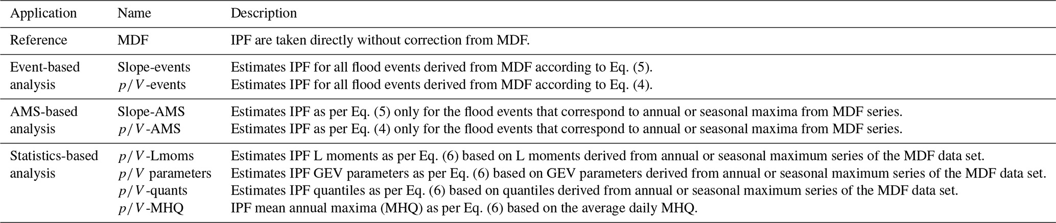
Another important point to be considered is that most of the studies mentioned above investigate the performance on the IPF maximum series and pay little attention to how these methods estimate the design flows with specific return periods. The general assumption is that, if the IPF maximum series are estimated well enough on average, so are the IPF quantiles. However, a well-estimated average IPF maximum may still lead to underestimation of design flows with a high return period (say 100 years). It makes sense to also investigate whether linear models based on MDF moments, parameters, or quantiles are more favourable for the estimation of the IPF quantiles. Accordingly, $p/V$ models are employed here to correct MDF information at different levels: correction of individual flood events from MDF, correction of MDF annual or seasonal maximum series, and direct correction of MDF-derived statistics (like mean maximum flow, L moments, distribution parameters, or even flood quantiles).

In this study, the linear models based on the $p/V$ as the key predictor (referred to here as $p/V$ models) are developed and assessed based on flow data from 648 catchments in Germany (as described in Sect. 2). The description of the methods and models used here for the estimation of the IPF from MDF information is given in Sect. 3.2. We then analyse the performance of the models in two main parts: their ability to estimate the mean maximum flow (MHQ) (see Sect. 4.1) and their ability to estimate probability distributions and the respective design floods (see Sect. 4.2). For the best model achieved, an uncertainty estimation is tackled by means of spatio-temporal resampling (see Sect. 4.3). Finally, the range and limitations of the proposed methodology and conclusions are given in Sects. 5 and 6, respectively.

2 Study area and data

This study uses flow data from 648 catchments distributed over Germany as shown in Fig. 1. For the analyses, continuous average daily flows (MDF) and instantaneous peak flows provided for each month as monthly peaks (IPF) are available. The selected sites represent the data sets of the federal agencies, which provide online access to both data sets (Lower Saxony, Saxony-Anhalt, Saxony, Bavaria and Baden-Württemberg; see the Data availability section).

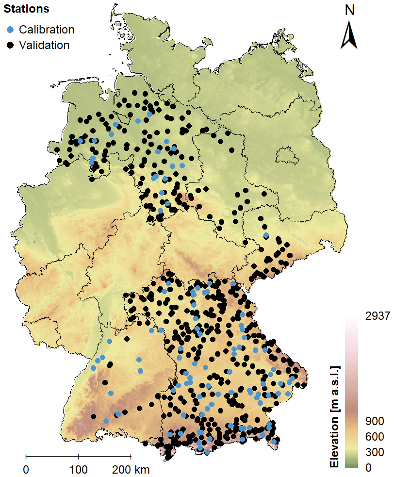
Figure 1 The spatial distribution of 648 catchments and their respective discharge gauges employed in this study. The 103 sites used for model calibration are marked in blue. The elevation is shown in the background colours and is provided by Jarvis et al. (2008), while the borders of the German federal states are shown with black lines.

Germany forms a transition zone from an oceanic climate in the north-west to a humid continental climate in the south-east. The north-western parts are influenced by wet air and have mild winters, while the more south-eastern parts are drier and exhibit larger temperature ranges. The average temperature for the entire country is 8.9 °C, the monthly averages ranging between 0.4 °C in January and 18 °C in July (reference period 1981–2010; DWD, 2021). The average annual precipitation is 819 mm, where amounts generally decrease from west to east and in strong dependence on the topography. Annual rainfall sums are generally highest over the Alps right at the southern border and the various secondary mountain ranges. The flat continental east is the driest. Temporally, the summer months are wettest, with rainfall often occurring in convective events. Snowfall occurs between October and April, where the amount and depth of snow cover increase with decreasing oceanic influence and increasing altitude.

Even though the entire area of Germany is not covered by the available data, the selected sites provide a cross section through the climatically and topographically distinct regions, from the flat oceanic north-west to the mountainous continental south-east.

The lengths of the discharge records vary substantially from 11 to 183 years, with a mean of 48.4 years (temporal span from 1831 to 2021). For the general assessment of differences in IPF and MDF floods and final model validation, all 648 sites with their variable record lengths are considered. For the assessment of flood frequency criteria, only sites with at least 30 years of observations are used (486). Model fitting (herein referred to as calibration) was carried out on a subset of 103 sites, whose discharge data were thoroughly checked. Also, their records were cropped to a common period from 1979 to 2012 to eliminate potential non-stationary effects. For the 103 sites used for calibration, a catalogue of catchment descriptors is available. For the remaining sites, only rudimentary information was obtained, i.e. catchment size, geographical position, and altitude of the gauges. Figure 2 shows how the 648 discharge gauges are distributed in terms of catchment size and elevation. It is evident that the majority of the sites have catchment areas under 500 km² and gauges situated at elevations higher than 100 m a.s.l.

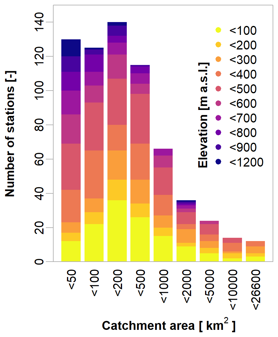
Figure 2 Distribution of catchment size and elevation for all 648 sites employed in this study.

3 Methods

3.1 Flood frequency analysis

FFA is applied to the two data sets for the available catchments in Germany: MDF and IPF. First, the maximum series are extracted from each data set either on an annual basis (AMS) or for each season of summer and winter (seasonal maximum series). For extrapolation of the maximum series and estimation of floods with specific return periods, distributions are fitted to the annual and seasonal samples of both IPF and MDF data sets. This enables the direct comparison of both flood quantiles and distribution parameters. For this study, the general extreme value distribution (GEV) of the following form is used for all the samples (Maidmennt, 1993):

$$\begin{array}{}\text{(1)}& F\left(x\right)=\exp \left\{-{\left[\mathrm{1}-{\displaystyle \frac{\mathit{\kappa }\cdot (x-\mathit{\xi })}{\mathit{\alpha }}}\right]}^{\frac{\mathrm{1}}{k}}\right\},\end{array}$$

with location parameter ξ, scale parameter α, and shape parameter κ. The parameters are estimated using sample L moments (Hosking and Wallis, 1997). The GEV has been proven before to be a suitable distribution for different catchments in Germany, as indicated by Haktanir and Horlacher (1993), Villarini et al. (2011), Ding et al. (2015), Ding et al. (2016) and Ding and Haberlandt (2017), and therefore it has been chosen in our study as well. The goodness of fit of the distributions is determined with the Cramér–von Mises test.

When extracting AMS, different flood peaks of different genesis (i.e. from convective or stratiform rainfall, from snowmelt, and so on) are mixed together and described by a single GEV distribution. However, if a certain flood type is dominating the annual maximum sample but is not typical for extremely large floods, then the fitted GEV distribution becomes misleading. To consider the different genesis in the flood peaks, maximum series are derived here for two seasons: summer (May–October) and winter (November–April). Then, a mixed model is applied, which combines two GEV distributions fitted to each of these sub-samples of the data: summer and winter floods. A simple maximum-mixing approach is used to combine the individual distributions to assess the annual non-exceedance probability of specific flood values:

$$\begin{array}{}\text{(2)}& F_{\mathrm{mix}}\left(x\right)=\prod _{i=\mathrm{1}}^n{f}_i\left(x\right),\end{array}$$

with f_i(x) as the annual non-exceedance probability calculated for each sub-sample (summer and winter) and F_mix(x) as the mixed-model annual non-exceedance probability for a flood value x. This approach allows the combined estimation of flood quantiles from multiple underlying distributions and thus the assessment of errors in seasonal FFA. The approach is described in detail in Fischer et al. (2016). In their study, they used thresholds to determine whether a seasonal maximum was actually a flood event, which may not be the case during dry summers. This threshold was defined as the minimum annual maximum flow. We do not censor our data with thresholds. That is, for matters of simplicity, we assume that every seasonal maximum is indeed a flood event.

3.2 Analysis and estimation of IPF

3.2.1 Calculation of the $p/V$ predictor from mean daily flows

Motivated by the recent findings of Fischer et al. (2016) and Fischer (2018) regarding different flood types, here the $p/V$ extracted from MDF is considered an important predictor that can help to estimate more accurately the IPF series from the MDF ones. This ratio is computed for each flood event extracted from the MDF data set as shown by Eq. (3):

$$\begin{array}{}\text{(3)}& p\backslash V\left({\displaystyle \frac{\mathrm{1}}{d}}\right)={\displaystyle \frac{Q_{\mathrm{dir}}\left[{\mathrm{m}}^{\mathrm{3}}\left[{\mathrm{d}}^{-\mathrm{1}}\right]\right]}{{\mathrm{Vol}}_{\mathrm{dir}}\left[{\mathrm{m}}^{\mathrm{3}}\right]}},\end{array}$$

where $p/V$ is the peak-to-volume ratio, Q_dir the direct peak flow, and Vol_dir the direct flood volume. Both Q_dir and Vol_dir are calculated for flood events extracted from MDF series (see below) after subtracting the baseflow.

To separate the flood events from the MDF, the initial steps of the procedure used by Tarasova et al. (2018) are carried out, which have been proven to be effective and convenient for the German catchments. For the initial step of baseflow separation, they selected the simple non-parametric algorithm provided by the Institute of Hydology (1980), which is able to identify the starting points of events in daily flow series in a wide range of catchments. The same method is applied to the series of mean daily flows in our study, which involves the following steps. First, 5 d non-overlapping blocks are used to find the minima, which are identified as turning points if they are more than 1.1 times smaller than their neighbouring minima. The baseflow is then derived by simple linear interpolation between the turning points. Discharge peaks are subsequently determined from the flow series, and for every peak the start and end of the respective flow event are defined by the nearest surrounding turning points. To prevent false identification of events due to natural variability, events are discarded if their peak discharge is not at least 10 % larger than the baseflow. Tarasova et al. (2018) suggested a second step of re-defining events with multiple peaks in an iterative procedure. This step is not carried out here, as it requires rainfall and snowmelt information, which is not available in our case. It is assumed that most of the events, especially the larger ones relevant for FFA, are separated correctly.

3.2.2 Estimation of instantaneous peak flows

In this study, we propose linear models to estimate IPF from the MDF data, where the peak-to-volume ratio (as described in Eq. 3) is one of the main predictors (referred to here as $p/V$ models). Other predictors that describe the catchment physiology or climate (referred to for simplicity as catchment descriptors) are also integrated and investigated. The combination of hydrograph shape and catchment characteristics as predictors is expected to better reproduce both the on-site and between-site variabilities in the IPF–MDF relationship and yield a more universal model. Several catchment descriptors describing land use, soil type, average climate variables, geographic information, and catchment morphology were investigated prior to the study. Two main descriptors, i.e. basin area and gauge elevation, were found to be more important for the linear model and hence are included in the study as shown here.

Since the $p/V$ ratio is calculated for each event, the first $p/V$ model investigated aims to correct individual flood events from MDF series. All events that contain maximum instantaneous monthly peaks are identified. For these events, the daily MDF_event and instantaneous IPF_event peaks as well as the $p/V_{\mathrm{event}}$ are computed. Then, a linear model of the following form is fitted:

$$\begin{array}{}\text{(4)}& {\mathrm{IPF}}_{\mathrm{event}}={\displaystyle \frac{{\mathrm{MDF}}_{\mathrm{event}}}{a+b_{\mathrm{1}}\cdot p\backslash V_{\mathrm{event}}+b_{\mathrm{2}}\cdot {\mathrm{CD}}_{\mathrm{1}}+\mathrm{\dots }+b_{n+\mathrm{1}}\cdot {\mathrm{CD}}_n}},\end{array}$$

where CD denotes additional catchment and climate descriptors that may be included in the models, and a and b are the parameters of the linear model fitted by the calibration procedure. The fitting of the model parameters is performed on the calibration set (as indicated in Sect. 2) only for the period 1972–2012.

To assess the performance of the new methodology, we also employ here the slope method developed by Chen et al. (2017) as a reference. The slope method estimates an IPF_event based on the slopes of the daily peak Q_peak to its preceding Q_pre and following daily flows Q_suc as shown in Eq. (5):

$$\begin{array}{}\text{(5)}& {\mathrm{IPF}}_{\mathrm{event}}=Q_{\mathrm{peak}}+{\displaystyle \frac{\left(Q_{\mathrm{peak}}-Q_{\mathrm{pre}}\right)\cdot \left(Q_{\mathrm{peak}}-Q_{\mathrm{suc}}\right)}{\mathrm{2}\cdot Q_{\mathrm{peak}}-Q_{\mathrm{pre}}-Q_{\mathrm{suc}}}}.\end{array}$$

Both of these estimation methods need information from the MDF hydrograph selected for each flood event observed. Hence, these methods can be applied in two ways: (1) IPF are estimated for all separate events in the average daily flow (MDF) series, even if these events have small daily peaks. Then, the flood frequency analysis is performed on the estimated event-based IPF (after selecting the maximum events for each year or season). (2) IPF are estimated for the maximum daily peak only. This means that the event hydrograph corresponding to the annual or seasonal daily maximum is considered for the calculation of $p/V$ in Eq. (4) or the peak discharges in Eq. (5). The obtained annual or seasonal maximum series are then used as a basis for the flood frequency analysis. In both cases, statistics are derived from the estimated IPF series and compared to the observed IPF ones. Procedure (1) is theoretically more accurate, since maxima in IPF and MDF do not necessarily occur at the same time (no temporal overlap). More precisely, events with maximum instantaneous peaks can have rather small mean daily peaks in some instances. Correcting only the maximum MDF would lead to underestimation of the IPF in these cases. On the other hand, Procedure (2) may prove more robust in cases where smaller events are not properly separated. That is, their volumes are overestimated or underestimated. These events would lead to unrealistic IPF estimates when using $p/V$ as a primary predictor. The larger events containing the annual maximum MDF are expected to be more properly separated by the algorithm described above.

Alternatively to the event-based estimation, the proposed $p/V$ model can also be applied directly to the MDF-derived statistics with the aim of reproducing the IPF statistics. These involve the estimation of flood statistics, i.e. MHQ, sample L moments, estimated distribution parameters, and derived flood quantiles based on averaged peak-to-volume ratios ($p/V_{\mathrm{mean}}$). These average $p/V$ ratios are obtained from all the annual and seasonal maximum MDF events at each site. As described above, these maximum events are expected to be properly separated, and although the maximum MDF events may not necessarily be identical to the maximum IPF events, their shape may hold important information about local processes. The model set-up is analogous to the event correction approach:

$$\begin{array}{}\text{(6)}& {\mathrm{IPF}}_{\mathrm{stat}}={\displaystyle \frac{{\mathrm{MDF}}_{\mathrm{stat}}}{a+b_{\mathrm{1}}\cdot p\backslash V_{\mathrm{mean}}+b_{\mathrm{2}}\cdot {\mathrm{CD}}_{\mathrm{1}}+\mathrm{\dots }+b_{n+\mathrm{1}}\cdot {\mathrm{CD}}_n}},\end{array}$$

where “stat” is the desired statistic being estimated, CD the selected catchment or climate descriptors, a and b the parameters of the model as fitted to the calibration set, and $p/V_{\mathrm{mean}}$ the average $p/V_{\mathrm{event}}$ for annual or seasonal series. The model is expected to represent the average conditions that determine the average deviation of MDF from IPF estimates. $p/V_{\mathrm{mean}}$ in itself is expected to be a good predictor that reflects local conditions like spatial scale, climate, geology, and other external factors that control flow variability obtainable from daily flow records. The additional inclusion of catchment descriptors is tested case by case and may contribute to the reproduction of the spatial variability of the target variable.

An overview of all the methods employed here together with their descriptions is given in Table 1. All methods consisting of the linear models based on the $p/V$ ratio as the main predictor ($p/V$ methods) have been optimized based on the calibration set only for the period 1972–2012. To select the best model, the coefficient of determination (R²) and the significance of the model parameters (based on the p value) are considered. For validation, all the sites with their respective observed periods are used. Through the validation we compare and assess the ability of the proposed models to capture the MHQ and the probability distribution and respective design floods.

Table 1 Description of all the methods employed here for the computation of IPF series and their respective statistics.

3.2.3 Analysis of the instantaneous peak flows

Since the IPF series are not continuous but rather one maximum per month (see Sect. 2), a direct comparison for each flood event is not possible. Instead, we focus here on the analysis of flood statistics. For this purpose, the general differences between IPF statistics IPF_stat and MDF-estimated flood statistics MDF_stat are calculated as follows:

$$\begin{array}{}\text{(7)}& \mathrm{error}\left(\mathit{\%}\right)={\displaystyle \frac{{\mathrm{MDF}}_{\mathrm{stat}}-{\mathrm{IPF}}_{\mathrm{stat}}}{{\mathrm{IPF}}_{\mathrm{stat}}}}\cdot \mathrm{100},\end{array}$$

where the error is computed at each site for any desired statistical quantity, like MHQ, L moments (Hosking, 1990), distribution parameters, and flood quantiles.

Apart from the error (%) at each site, two additional performance criteria are calculated over all the sites: the normalized root mean square error (nRMSE) as per Eq. (8 and the percent bias (pBIAS) as per Eq. (9):

$$\begin{array}{}\text{(8)}& {\displaystyle }& {\displaystyle }\mathrm{nRMSE}\left(\mathit{\%}\right)=\mathrm{100}\cdot {\displaystyle \frac{\sqrt{\frac{\mathrm{1}}{N}\cdot \sum _{i=\mathrm{1}}^N{\left({\mathrm{MDF}}_{{\mathrm{stat}}_i}-{\mathrm{IPF}}_{{\mathrm{stat}}_i}\right)}^{\mathrm{2}}}}{{\mathrm{sd}}_{{\mathrm{IPF}}_{\mathrm{stat}}}}},\text{(9)}& {\displaystyle }& {\displaystyle }\mathrm{pBIAS}\left(\mathit{\%}\right)={\displaystyle \frac{\sum _{i=\mathrm{1}}^N{\mathrm{MDF}}_{{\mathrm{stat}}_i}-{\mathrm{IPF}}_{{\mathrm{stat}}_i}}{\sum _{i=\mathrm{1}}^N{\mathrm{IPF}}_{{\mathrm{stat}}_{\mathrm{i}}}}},\end{array}$$

where N is the number of validation sites, MDF${}_{{\mathrm{stat}}_i}$ and IPF${}_{{\mathrm{stat}}_i}$ are the respective statistics from MDF and IPF series, and sd${}_{{\mathrm{IPF}}_{\mathrm{stat}}}$ is the standard deviation of IPF statistics over all the considered sites. These criteria are computed for each of the methods described in Table 1.

3.3 Uncertainty analysis

Since both the distribution fitting and the IPF estimation via $p/V$ models are approximations and not fully accurate, we eventually assess the overall level of uncertainty in the final IPF flood quantile estimates. As will be shown later in Sect. 4.2, the best correction approach is chosen to be the $p/V$-Lmoms – the model directly correcting the L moments of the MDF series. This is done using simple resampling with replacement procedures, resampling in time when selecting the maximum series for FFA, resampling in space when selecting the sites for the $p/V$ model (either for calibration or validation of the models), and resampling in both space and time. In the first step, the series of annual or seasonal maxima from both MDF and IPF data sets are analogously resampled 1000 times with replacement (temporal sample and parameter uncertainty). For each resampling, the desired flood quantiles are estimated using L moments. The range of these estimates provides the baseline level of uncertainty due to sample and parameter uncertainty. The temporal sample uncertainty is calculated at each site for the original IPF and MDF series (IPF-bs and MDF-bs, respectively) and is considered as a benchmark for comparison.

In the second step, $p/V$ models are fitted to each pairing of temporally resampled IPF and MDF series while considering all sites in the study area that have more than 30 years of observations. This means that the temporal sample uncertainty is propagated through the $p/V$ model ($p/V$-full). To assess the uncertainty of the selected $p/V$ model, another resampling is carried out, this time shuffling the set of considered sites, where the original MDF L moments are resampled again 1000 times with replacements before fitting the $p/V$ model ($p/V$-bs). Lastly, the total uncertainty in both space and time is assessed by combining the temporal sample and parameter uncertainty with the uncertainty of the fitted models: this means that the maximum series are resampled 1000 times, and for each of these sets, the sites are resampled 1000 times as well before fitting the $p/V$ model. So, the total uncertainty will be derived by 1000⋅1000 quantile estimates ($p/V$-bs-bs). Of course, the uncertainty ranges might change slightly if more realizations are included. For method comparison in terms of their uncertainty range, the number of random resamplings will influence all the methods similarly. On the other hand, 1000 realizations are enough to investigate the dominant sources of uncertainty. Finally, to capture the overall uncertainty, a previously conducted test showed that 1 000 000 realizations are enough to capture the overall trends of the uncertainty.

To assess the overall level of uncertainty, several indices are computed at each site. The first one is the relative width of the 95 % confidence intervals (CIs) calculated for all the aforementioned resampling estimates of the desired flood quantile:

$$\begin{array}{}\text{(10)}& \mathrm{CI}\mathrm{95}{\mathit{\%}}_{\mathrm{bs}}={\displaystyle \frac{x_{\mathrm{bs},\mathrm{0.975}}-x_{\mathrm{bs},\mathrm{0.025}}}{x_{\mathrm{bs},\mathrm{0.5}}}},\end{array}$$

where x_bs,0.025 and x_bs,0.975 are the 2.5 % and 97.5 % quantiles and x_bs,0.5 is the median of the respective sample.

The second one is the deviation of the IPF-estimated samples from the IPF original sample, which allows the assessment of error distributions:

$$\begin{array}{}\text{(11)}& {\mathrm{error}}_{\mathrm{bs}}={\displaystyle \frac{x_{\mathrm{bs}}-{\mathrm{IPF}}_{\mathrm{bs}}}{{\mathrm{IPF}}_{\mathrm{bs}}}}\cdot \mathrm{100}\mathit{\%},\end{array}$$

where IPF_bs is the temporal resample of the IPF original data and x_bs is the resample estimated from either the original MDF series or the modelled IPF series. From the resulting error vector, a variety of statistics can be computed for comparison.

Finally, the agreement of the 95 % confidence intervals of the MDF and $p/V$ model samples with the IPF confidence bands is determined as the percentage overlap at each site:

$$\begin{array}{}\text{(12)}& \begin{array}{rl}& \mathrm{overlap}=\\ & {\displaystyle \frac{\min \left(X_{\mathrm{bs},\mathrm{0.975}},{\mathrm{IPF}}_{\mathrm{bs},\mathrm{0.975}}\right)-\max \left(X_{\mathrm{bs},\mathrm{0.025}},{\mathrm{IPF}}_{\mathrm{bs},\mathrm{0.025}}\right)}{\max \left(X_{\mathrm{bs},\mathrm{0.975}},{\mathrm{IPF}}_{\mathrm{bs},\mathrm{0.975}}\right)-\min \left(X_{\mathrm{bs},\mathrm{0.025}},{\mathrm{IPF}}_{\mathrm{bs},\mathrm{0.025}}\right)}}\\ & \cdot \mathrm{100}\mathit{\%},\end{array}\end{array}$$

where IPF_bs is the temporal resample of the IPF original data and x_bs is the resample estimated from either the original MDF series or the modelled IPF series.

4 Results

4.1 MHQ

4.1.1 Comparison of MDF and IPF

Figure 3 demonstrates the error in MHQ estimated by MDF instead of IPF series (as per Eq. 7) in relation to the catchment size and the geographic location. It is clear that the larger the area, the smaller the deviation between MDF and IPF. In these cases, the MDF are good representations of the IPF peaks. Moreover, MHQ errors shown in Fig. 3 appear to be especially large at higher altitudes. This is indeed as expected, as mountainous catchments have a fast response time and are generally more heavily influenced by the meteorological forcing (by snowmelt processes or convective events). Overall, the MHQ error in our catchments seems to increase in the north–south direction, which could be a secondary effect of both increasing altitude and decreasing catchment size.

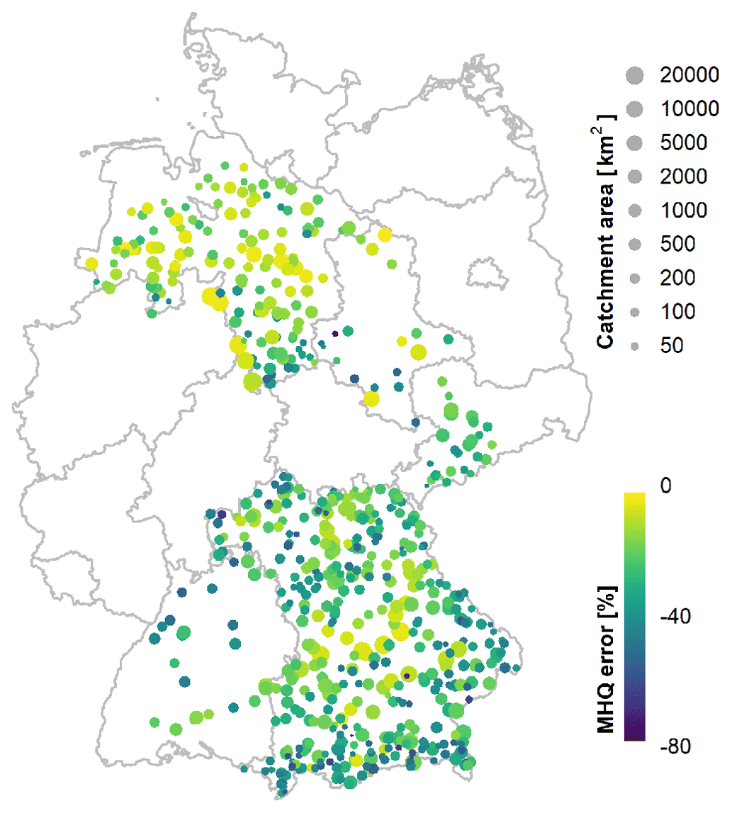
Figure 3 Spatial distribution of the mean annual maximum flow (MHQ) error (%) between mean daily (MDF) and instantaneous peak (IPF) flows obtained from all the sites (calculated as per Eq. 7).

When assessing the differences between mean daily and instantaneous peaks, it is also meaningful to take a closer look at different types of floods. For our German sites, the two most opposite types are (a) flood events induced by short intense rainfall, especially convective events dominant mainly in summer (May–October); and (b) extended flood events with a significant volume, as caused by snowmelt and/or stratiform rain occurring mainly in winter (November–April). Presumably, the latter flood type is much better represented by mean daily flow than the former. In order to roughly distinguish between the two types, the flow records are divided into summer (May–October) and winter (November–April) half-years. Due to the limited data availability, a clear distinction between convective, stratiform, and snowmelt events cannot be achieved here. Some snowmelt events in the high alpine catchments may still occur in May and June but are classified as summer events. However, the coarse division of the data into half-years rather than seasons is due to the subsequent analysis of seasonal flood statistics and application of the mixed seasonal model. In Fig. 4a–c, the MHQ error is shown for the entire year and also for the summer and winter seasons. The relationship with the catchment area is still clearly visible in all three cases. Also, the effect of the elevation becomes obvious, as sites at the lowest elevations (yellow points, below 100 m) show very small errors, even for small catchment sizes down to approximately 100 km². This is the clearest stratification in the error due to elevation; the errors at higher altitudes appear less distinguishable.

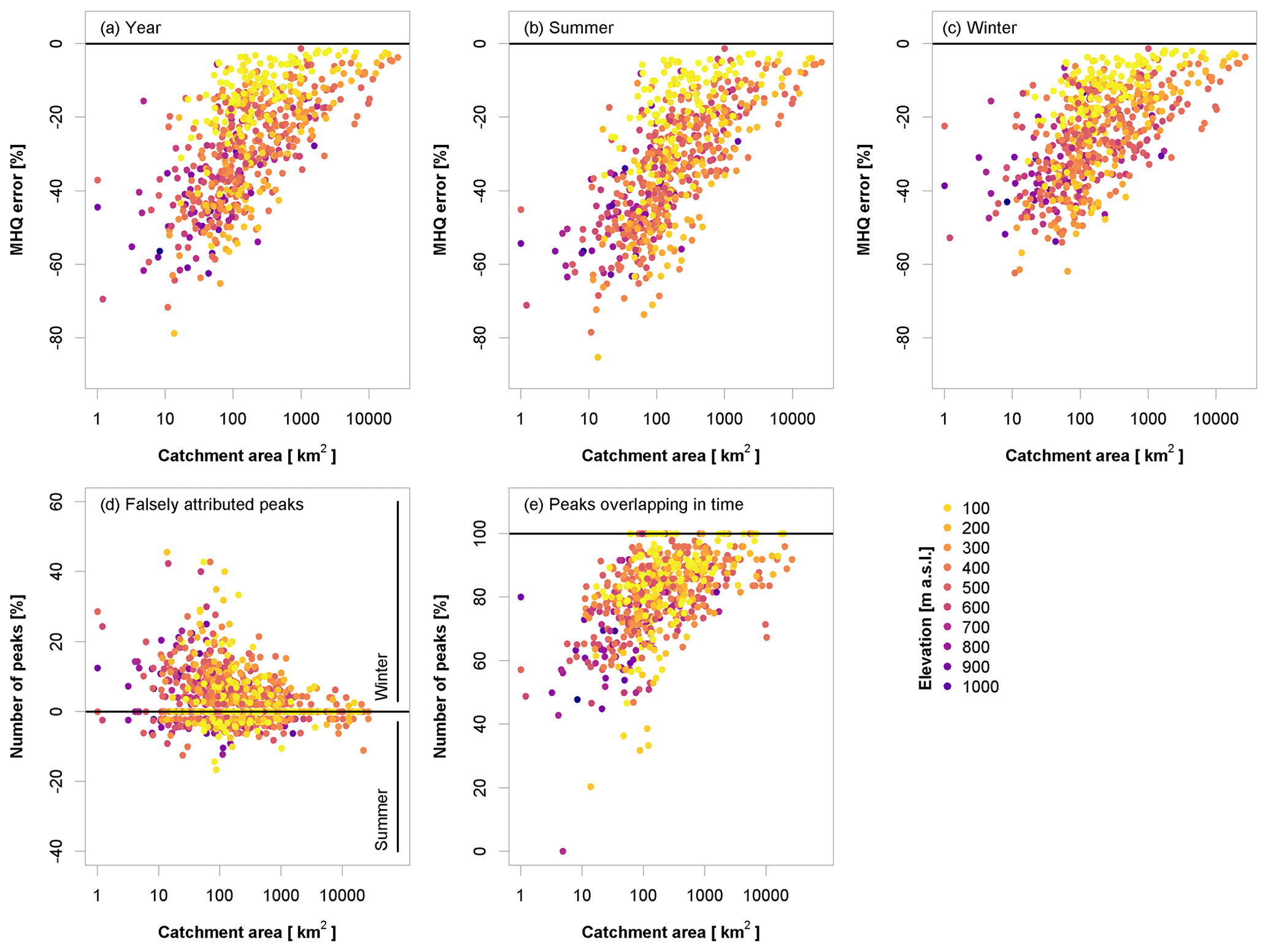
Figure 4 (a–c) Error (%) in the MHQ (as per Eq. 7) obtained in relation to catchment size and gauge elevation for the entire year (a), summer (b), and winter (c); (d, e) percentage of peaks falsely attributed by MDF to the winter or summer half-year (d) and percentage of peaks in MDF and IPF that overlap in time (within a 5 d buffer) (e). Results are illustrated for all the sites.

There is, however, a clear distinction between the summer and winter seasons. As expected, the MHQ error is smaller overall in the winter months, where snowmelt and stratiform events prevail, while the convective events in summer are poorly captured by MDF. The error in the annual peaks is a mixture of the two seasons: which season contributes more to the annual peaks depends on the individual flood regimes. When looking at the IPF data, at 68.8 % of the considered sites the winter floods exceed on average their summer counterparts, while 29.2 % of the sites are dominated by summer floods. When considering MDF instead, only 22.1 % of the sites are identified as having maximum peaks in summer. This indicates that the mean daily flow significantly smoothens the summer peaks to a point where they are no longer relevant for the overall flood behaviour. Figure 4d shows the percentages of annual maxima at each site that are attributed to the wrong season when using MDF. Each site is represented by two dots: negative values show the percentages of all annual maxima that are falsely attributed to summer, while positive values show the falsely attributed winter peaks. It is obvious that with decreasing catchment size an increasing number of annual maxima are falsely identified in the winter half of the year, while the actual instantaneous maxima occur in summer.

Another general issue highlighted by this analysis, independent of seasonality, is that the peaks of both the IPF and MDF data sets do not necessarily occur on the same day (there is no temporal overlap). In their study, Chen et al. (2017) illustrated that only for 82 % of the events investigated did the peaks of both IPF and MDF series occur on the same day. This suggests that instantaneous maxima are not always identifiable in the mean daily flows. That is, the maxima obtained from the daily series are inevitably found in other places. The temporal overlap of IPF- and MDF-derived peaks for our catchments is shown in Fig. 4e. In general, the smaller the catchment, the smaller the temporal overlap between instantaneous and daily peaks. This problem needs to be kept in mind when attempting to estimate instantaneous peaks from daily peaks, since the two may belong to significantly different events (different genesis) and thus to different populations.

4.1.2 Estimation of MHQ

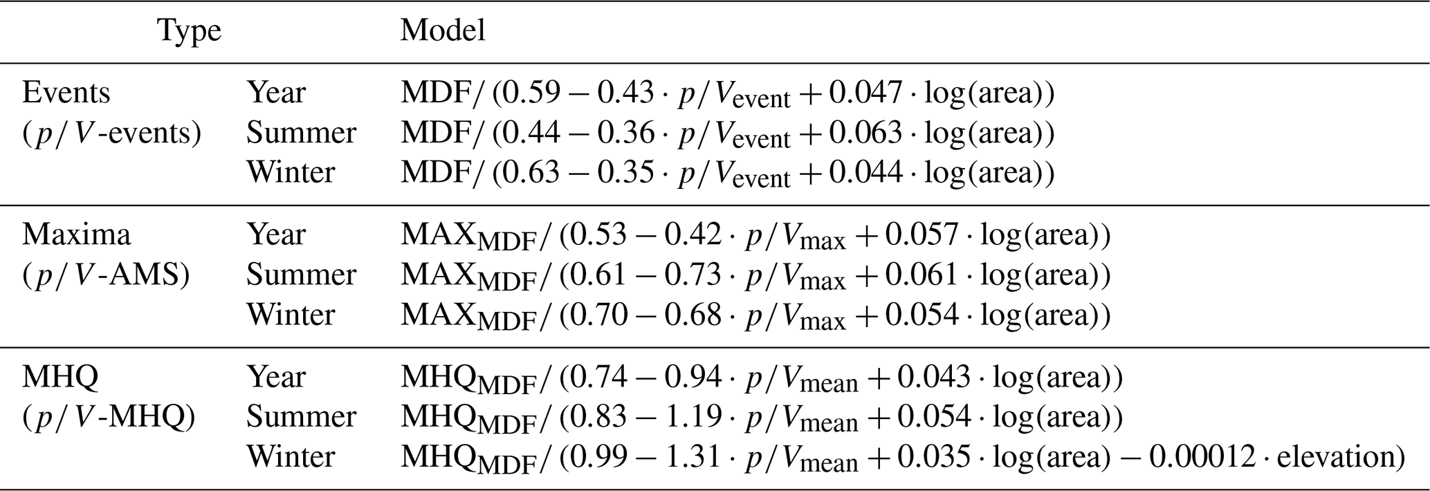
So far, the error in the MHQ between MDF and IPF has been shown to be influenced by both catchment area and gauge elevation. Both of these predictors may be helpful in correcting MDF for better agreement with the IPF data. Moreover, there seems to be a significant linear dependence between the peak ratios MDF / IPF, the $p/V$ ratio, and the logarithm of the catchment size. We first test the suitability of various predictors for predicting MHQ from IPF by fitting the $p/V$ models to the individual events of MDF ($p/V$-events), to the MDF maximum series ($p/V$-AMS), or, lastly, directly to the MDF mean maximum flow ($p/V$-MHQ). Various model combinations with the available predictors (catchment area, elevation, and $p/V$ ratio) are tested using the calibration data set, and their respective coefficients of determination are shown in Table 2. The selected models are marked in bold in Table 2, and their respective full-model formulas are given in Table 3. For most models, the majority of variances in the IPF–MDF relationship are explained by the $p/V$ ratio and the catchment area. For winter, including gauge elevation appeared to improve the model slightly.

Table 2 Coefficients of determination for various model combinations (see Table 1 for a description of the models). Values are obtained by fitting the models only to the calibration set. Bold numbers indicate the best $p/V$ model for each application, and asterisks indicate at least one non-significant predictor in the $p/V$ models.

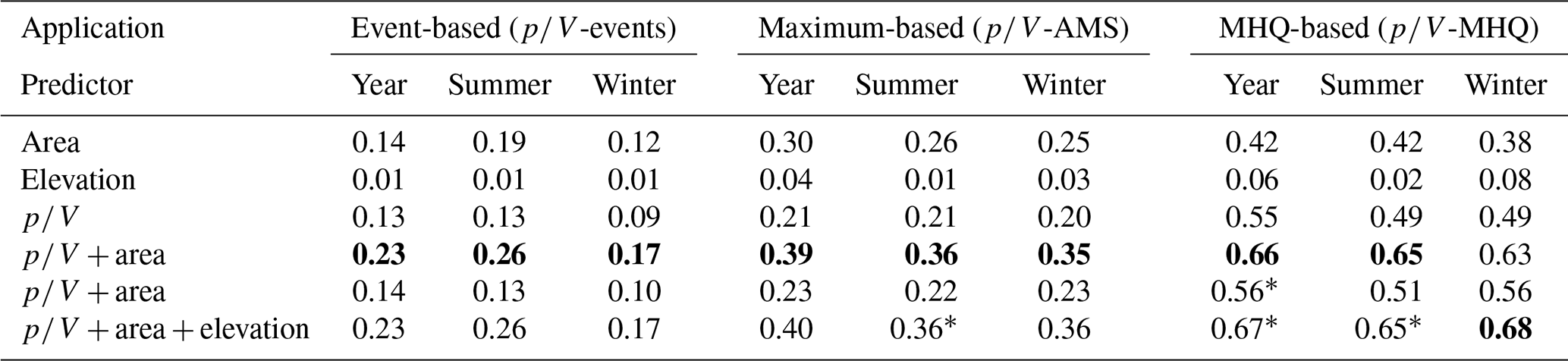
Table 3 The best $p/V$ models (as shown in bold in Table 2) fitted to the calibration set for correction of individual events ($p/V$-events), annual or seasonal maxima ($p/V$-AMS), and the MHQ ($p/V$-MHQ).

The models show a similar performance for the annual and summer peak ratios in both the correction of individual events ($p/V$-events) and the mean maximum flow ($p/V$-MHQ). For winter, the model performance seems to differ, especially when correcting the individual events ($p/V$-events). It appears that the models using the $p/V$ have more difficulty estimating the winter peak ratio. This could be due to improper event separation, which will be discussed in more detail below and which leads to unrealistic $p/V$ ratios. The fact that elevation is a significant predictor in the MHQ model ($p/V$-MHQ) may also suggest that the peak ratios in winter are more heterogeneous.

Figure 5 shows the change in mean absolute error in the annual MHQ after correction with the different methods in relation to catchment size and elevation: positive values indicate that the error has increased after correction, while negative values indicate that the error has decreased after correction. The slope method (Fig. 5a) applied to the individual events (slope-events) yields a rather constant reduction in the error independent of catchment size. However, there are several outliers produced by this method, which can be attributed to improper separation of smaller events. Applying the slope method only to the annual maximum MDF events (slope-AMS), as done in Fig. 5b, shows a much smoother and more constant error reduction. The corrections using the $p/V$ models proposed here (Fig. 5c–e) yield a much larger improvement for the smaller catchments (where the original MDF error was generally larger than in the bigger catchments). Nevertheless, these corrections simultaneously lead to an increase in the error in several cases. This deterioration appears to affect the sites that were highlighted before in Sect. 4.1.1, i.e. those with the lowest elevations in the data set where the original MDF error was quite low.

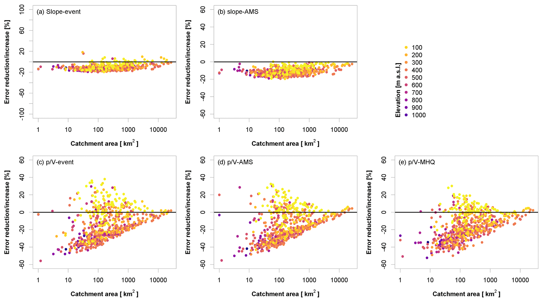
Figure 5 Error reduction (negative values) vs. error increase (positive values) in the MHQ for different IPF-estimation methods when compared to MDF. For an overview of the methods, the reader is directed to Table 1. Values are obtained by applying the selected methods to the validation set.

The differences between correcting the individual events ($p/V$-events) and the annual maxima ($p/V$-AMS) (as illustrated in Fig. 5c and d, respectively) by means of the $p/V$ models appear rather small. This suggests that even though the annual maximum from the MDF in many cases does not occur at the same time as the annual maximum from the IPF, the method still yields an appropriate estimate of the true IPF. On the other hand, directly correcting the MHQ ($p/V$-MHQ in Fig. 5e) results in a slightly lower error reduction for the smaller catchments but also appears to produce fewer outliers and is thus considered more robust.

It should be noted that working with large data sets and automatic event separation without manual post-correction leads to problems that could potentially be avoided when considering individual time series more carefully. Several events are identified as too long or too short (or not at all), so their volumes are overstated or understated, respectively. This results in false $p/V$ ratios and in some cases severe overestimation or underestimation of the peaks. The weight of such events is assumed to be significantly lower when correcting flood statistics based on average $p/V$ ratios. In addition, the overall performance can only be assessed for events that contain the monthly instantaneous maximum flow, i.e. primarily larger events. How the event correction performs for minor events cannot be analysed here.

Figure 6 summarizes the overall model performances to estimate the IPF MHQ at all the validation sites and compares the individual methods to the error using MDF directly. It is obvious that all the methods give significantly better IPF estimates than the MDF alone. The slope correction methods (both slope-events and slope-AMS) have quite a large bias (median error around −10 %), which is, as seen above, not only disadvantageous. Still, the overall error is smaller for the $p/V$ models ($p/V$-events, $p/V$-AMS, and $p/V$-MHQ), where the median error is 0 %–2 %, with fewer positive outliers produced by the $p/V$-MHQ approach.

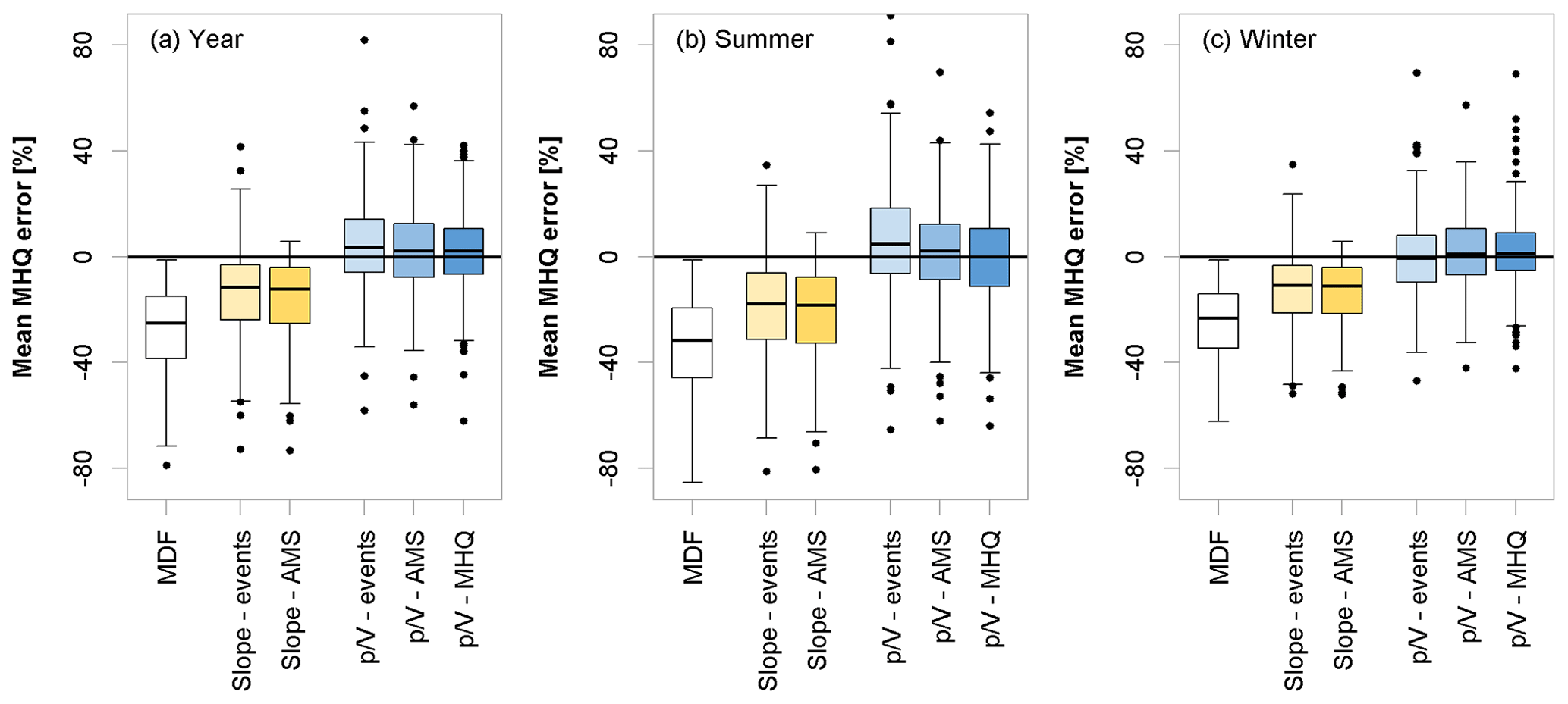
Figure 6 Error (%) comparison of different methods to estimate the mean MHQ for the entire year (a), summer (b), and winter (c). Values are obtained by applying the selected methods to the validation set. For an overview of the methods, the reader is directed to Table 1.

Table 4 summarizes the nRMSE (%) and pBIAS (%) of the MHQ estimated by the different model variants. In terms of nRMSE, the performances of the slope and $p/V$ methods are comparable, with the slope methods being more biased. There are a number of outliers produced by the $p/V$ methods, especially positive ones, that affect the overall nRMSE. As seen in Fig. 5, this primarily concerns the low-elevation catchments below 100 m. The values in parentheses in Table 4 indicate the performance criteria for gauges with catchment areas under 500 km². Here, the advantage of the $p/V$ approaches over the slope methods becomes apparent even though a large number of low-elevation catchments fall into this category, which negatively affects the overall error.

Table 4 Normalized root mean square error (nRMSE, %) and percentage bias (pBIAS, %) of estimated vs. observed instantaneous MHQ over all validation sites for different methods. The values in parentheses show the performances for catchment sizes under 500 km².

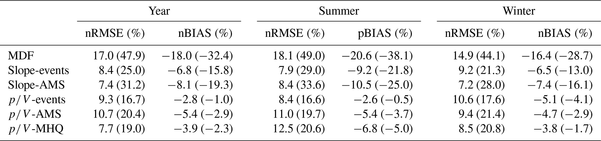
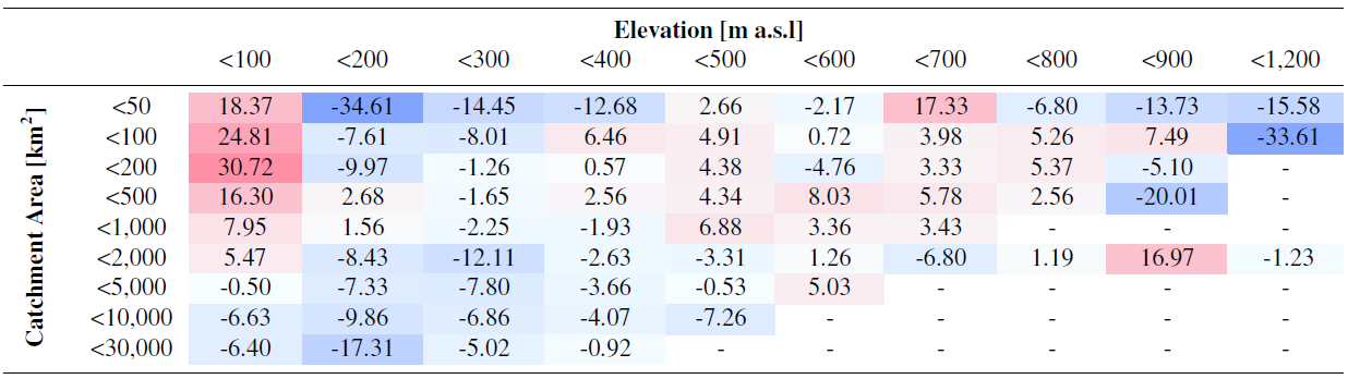
Table 5 Average prediction error (%) of the $p/V$-MHQ model for the annual MHQ calculated over the validation sites and shown here for different ranges of area and elevation. Red shades indicate overestimation, blue shades underestimation.

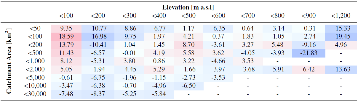
Table 5 shows the average error between the annual MHQ predicted by the $p/V$-MHQ model with the observed instantaneous annual MHQ, distributed for different catchment sizes and elevations. It becomes obvious that, for the lowest elevations, the instantaneous annual MHQ is overestimated, especially for smaller catchment sizes. Catchments in the range of 100 to 200 m altitude also show quite large errors, but these are mostly negative. It is also apparent that the catchments with outlets at higher elevations exhibit large negative errors in most cases.

4.2 Probability distributions and derived design flows

So far, the proposed $p/V$ models have been analysed in terms of their ability to better estimate the MHQ from MDF data. In this sub-section, the focus is shifted to the ability of the methods to estimate the parameter distribution of the IPF and the derived flood quantiles. The GEV distribution appears to be a generally suitable distribution for the sites in the data set. A Cramér–von Mises test is carried out for the original IPF and MDF samples as well as for the slope and $p/V$-corrected samples at each site, and they are certified to be a good fit in all cases (p value = 5 %).

4.2.1 Comparing MDF and IPF distributions

A comparison between the estimated parameters for the IPF and MDF samples for the year and the seasons is shown in Fig. 7. As expected, the location parameters are consistently underestimated by the MDF series, with the largest errors in summer. This naturally leads to an overall downward shift of the “true” distribution when estimated from MDF values. The scales, normalized here by the location, appear to be primarily overestimated in summer, leading to distributions that are steeper for MDF samples than for IPF samples. For the year and winter, the errors in the scale parameters appear to be balanced in their directions. The shape parameters differ quite substantially between the seasons. In summer, the vast majority of the estimated parameter values are negative in both IPF and MDF. This indicates a heavy-tail behaviour for the summer floods. The fact that these negative values are in many cases smaller in the MDF sample than in the IPF sample suggests that the tails are overstated in the former case. For the year and winter season, again, no clear trend is visible. The distribution parameters of the low-elevation gauges appear to be very well-estimated by the MDF. For the higher elevations, the estimation of the shape parameters seems especially difficult. For the whole year, the IPF shape is underestimated at a lot of the gauges, while it is primarily overestimated in winter. Overall, due to the underestimation of the location parameter, underestimation of both lower and higher flood quantiles by the MDF sample is expected.

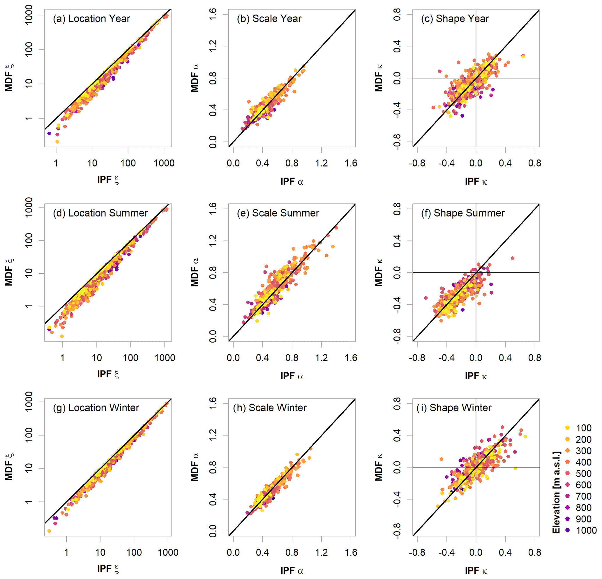
Figure 7 Estimated generalized extreme value (GEV) parameters from the IPF vs. MDF annual or seasonal maximum series. Here, only validation sites with observations longer than 30 years are shown.

Generally, the heavy tails of the summer distributions, in contrast to the flatter tails in winter, let the summer floods become dominant at higher quantiles. For a return period of 100 years, the summer floods exceed the winter peaks at 61.9 % of the sites. For 50 and 10 years, this exceedance occurs at 51.2 % and 35.7 % of the sites. This behaviour is also noticeable in the MDF but for fewer gauges, i.e. 53.4 %, 43.2 %, and 21.0 % for 100-, 50-, and 10-year return periods.

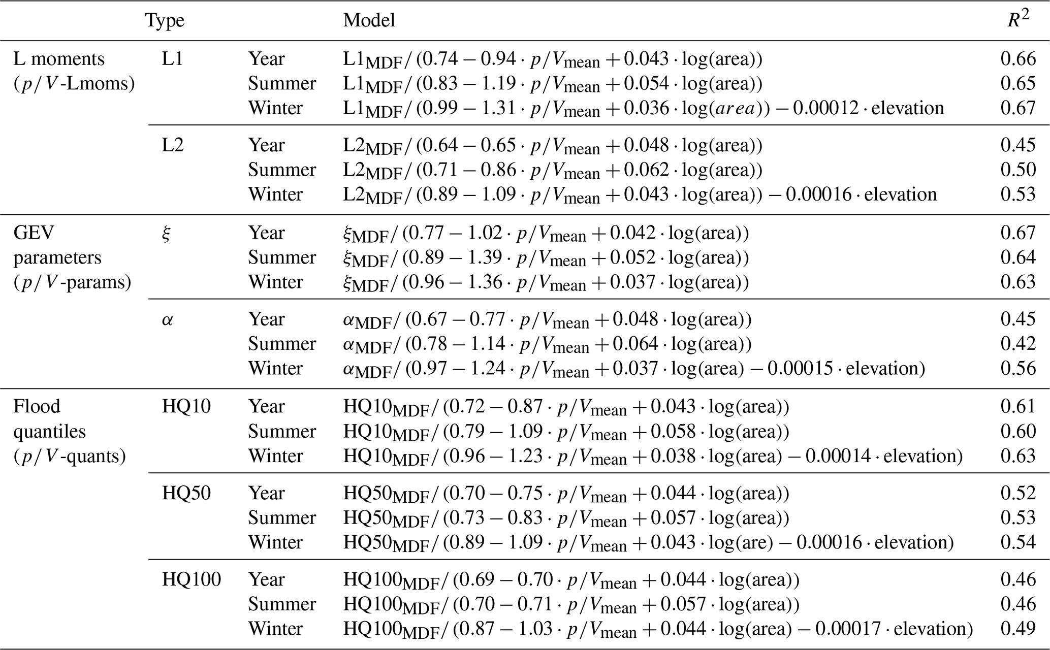
Table 6 $p/V$ models fitted to the calibration data set for correction of L moments ($p/V$-Lmoms), GEV parameters ($p/V$-params), and flood quantiles ($p/V$-quants) derived from the MDF annual or seasonal maximum series. For an overview of the methods, the reader is directed to Table 1.

4.2.2 Estimation of IPF distributions and quantiles

Three approaches were tested to estimate IPF flood quantiles based on MDF statistics: (a) correcting the sample L moments required for parameter estimation ($p/V$-Lmoms), (b) correcting the parameters of the fitted distribution ($p/V$-params), and (c) directly correcting the desired flood quantiles ($p/V$-quants). Method (a) is convenient, since a single model for each L moment facilitates a correction of the complete distribution and hence each desired flood quantile. Estimating the L moments has the additional advantage of not being restricted to a certain type of probability distribution. A proper distribution can be selected and fitted locally using the corrected L moments. Still, the other methods may prove more robust and are hence tested as well. The final models for each target variable are selected according to the procedure for the MHQ (see Table 2) using the calibration data set. For reasons of conciseness, only the final models are presented in Table 6.

For further comparisons, distributions were also fitted to the annual and seasonal maxima that were previously corrected using the slope (slope-events) and $p/V$ methods for events ($p/V$-events). Since the shape parameter is generally difficult to estimate, especially for such a short time period, and the models' estimates are generally close to the observed MDF shape parameter, it will not be estimated using the model variants. Instead, the MDF shape parameter estimate will be used in all instances. Figure 8 shows the errors (%) in GEV-parameter estimates for the different approaches in comparison to the original uncorrected MDF error (%) computed over the 486 validation sites with a minimum of 30 years of observations. Since the $p/V$-quants method directly corrects the MDF quantiles, it cannot be used to estimate the GEV parameters and hence is not illustrated in Fig. 8. All the methods shown clearly improve the estimation for the location and scale parameters when compared to the original MDF estimates. The corrections based on the $p/V$ models proposed here ($p/V$-events, $p/V$-Lmoms, and $p/V$-params) are less biased than the slope method (slope-events) proposed by Chen et al. (2017). Particularly the correction of the MDF sample L moments ($p/V$-Lmoms) shows the smallest error and bias.

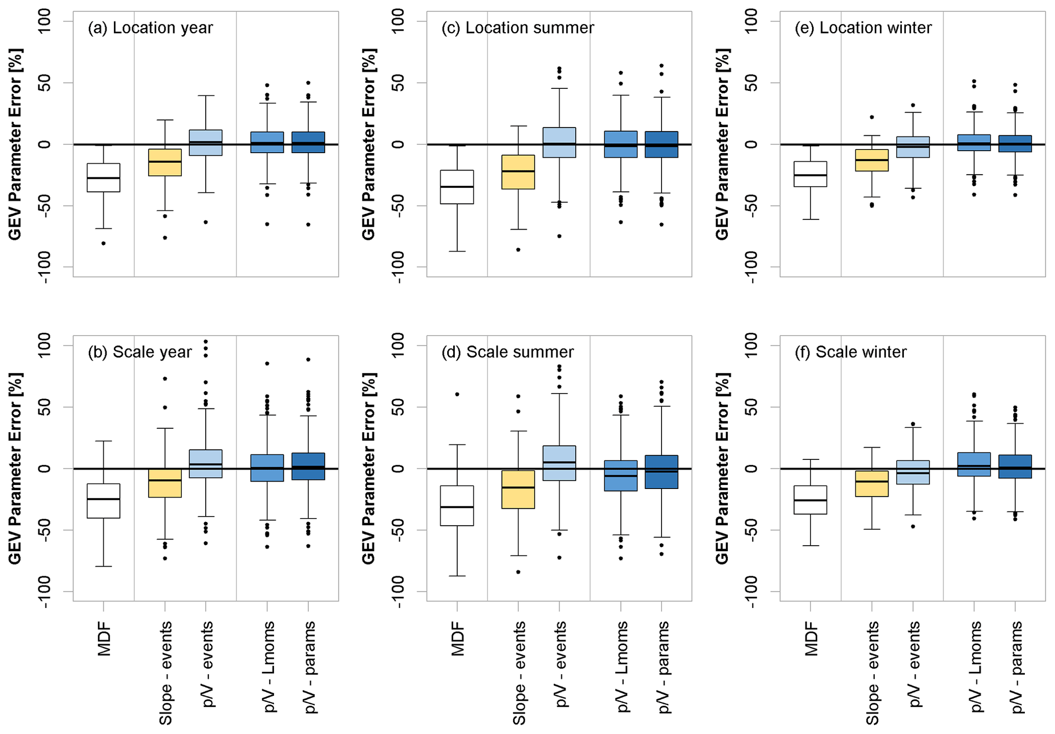
Figure 8 Error (%) comparison of various IPF-estimation methods (see Table 1 for an explanation of the methods) regarding their ability to estimate GEV distribution parameters based on annual or seasonal maximum series. Only validation sites with more than 30 years of observations are used for the boxplots.

Figure 9 demonstrates the quality of the different correction approaches for the 10-, 50-, and 100-year floods at the 486 validation sites. With increasing return periods, the performance of all the correction methods appears to decline. Differences in the tails of the fitted distributions are more difficult to capture with the analysed approaches. This turns out to be especially valid for the low-altitude catchments. The overcorrection that was observed for the mean is even more pronounced here, which leads to an average decline in model performance. Also, the general uncertainty in parameter estimation and extrapolation far beyond the time series length needs to be kept in mind. Overall, even the estimation of the “true” IPF quantiles is potentially defective in itself, as will be discussed in the next section.

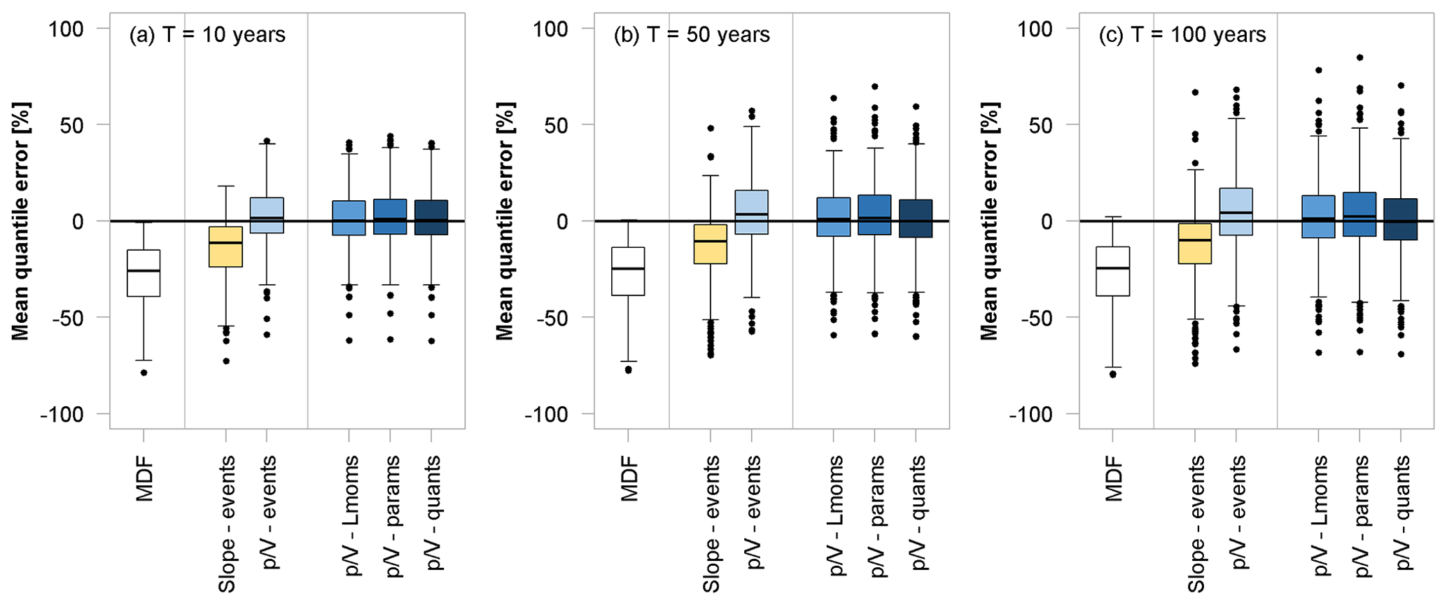
Figure 9 Error (%) comparison of various IPF-estimation methods (see Table 1 for an explanation of the methods) regarding their ability to estimate different flood quantiles based on annual maximum series. Only validation sites with more than 30 years of observations are used for the boxplots.

Table 7 Performance of different IPF-estimation methods in terms of nRMSE (%) and pBIAS (%) for different flood quantiles estimated from annual maximum series. The performance is computed over validation sites with more than 30 years of observations, while the values in parentheses show the performance for catchment sizes under 500 km². For a description of the methods shown here, see Table 1.

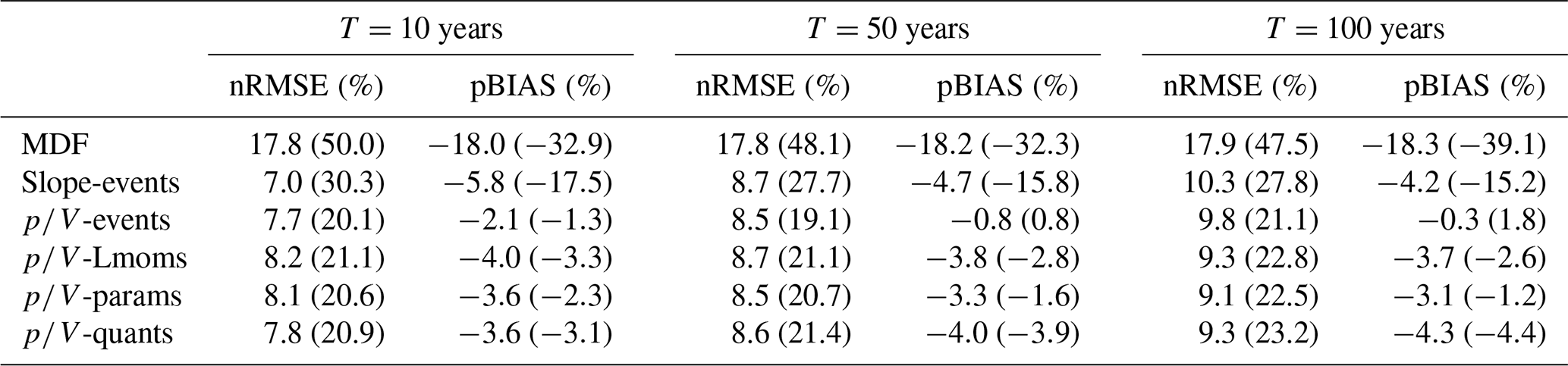
Table 8 Average prediction error (%) of the $p/V$-Lmoms model for the 100-year flood (HQ100) calculated over the validation sites and shown here for different ranges of catchment area and gauge elevation. Red shades indicate overestimation, blue shades underestimation.

Since the average $p/V$ ratio is used for the direct correction of L moments, parameters, and flood quantiles, it is expected that the performance will decrease with increasing return periods, as the $p/V_{\mathrm{mean}}$ may not relate much to the higher quantiles. Still, even for the 100-year flood, these approaches appear to work just as well as the $p/V$-events approach, as also indicated by the performance criteria (nRMSE, %, and pBIAS, %) given in Table 7. The performance of all three methods is comparable, but due to its previously mentioned advantages, the L-moment method ($p/V$-Lmoms) is considered the superior approach in this setting. Among the event correction techniques, the slope method performs similarly to the $p/V$ method in terms of overall error but is again more biased. When focusing on the catchments with areas under 500 km², the superiority of the $p/V$ methods becomes apparent.

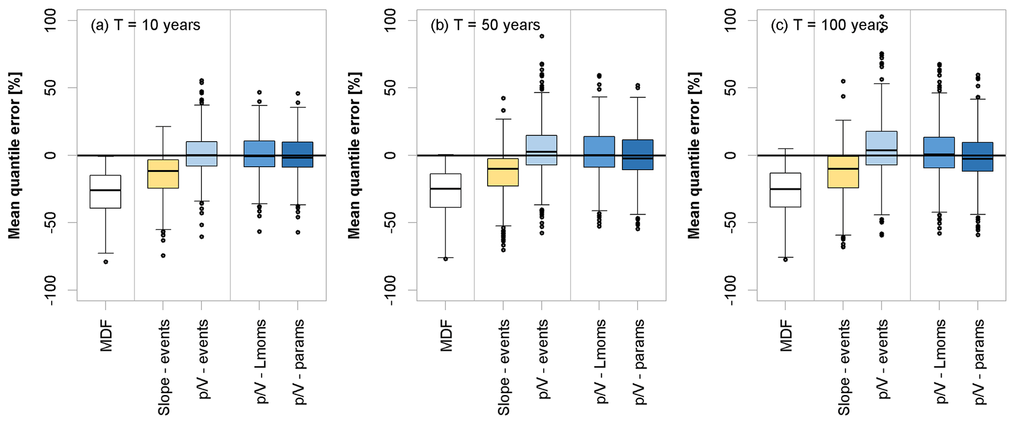
Figure 10 Error (%) comparison of various IPF-estimation methods (see Table 1 for an explanation of the methods) regarding their ability to estimate different flood quantiles based on a mixed model of seasonal maximum series. Only validation sites with more than 30 years of observations are used for the boxplots.

The distribution of the prediction error for the correction of L moments ($p/V$-Lmoms) over the different catchment areas and elevations can be found in Table 8. The errors are exemplarily shown for the 100-year flood. The error distribution is comparable to the MHQ shown in Table 5. Again, the overestimation for the lowest elevations is especially striking, as is the significant underestimation at higher altitudes.

Finally, the model performance of the mixed models, combining summer and winter floods, is analysed for different flood quantiles. Their behaviour is generally comparable to the annual maximum series approach, as shown in Fig. 10. Even though the quantiles obtained with the mixed models may be more extreme and more parameters may need to be estimated and corrected, there is no indication that the IPF correction will not function in this case. The nRMSE (%) and pBIAS (%) values for the mixed models are shown in Table 9. According to these values, the event correction methods appear to perform best overall. For the smaller catchments (<500 km²), the $p/V$ methods outperform the slope method.

Table 9 Performance of different IPF-estimation methods in terms of nRMSE (%) and pBIAS (%) for different flood quantiles estimated from mixed models of seasonal maximum series. The performance is computed over validation sites with more than 30 years of observations, while the values in parentheses show the performance for catchment sizes under 500 km². For a description of the methods shown here, see Table 1.

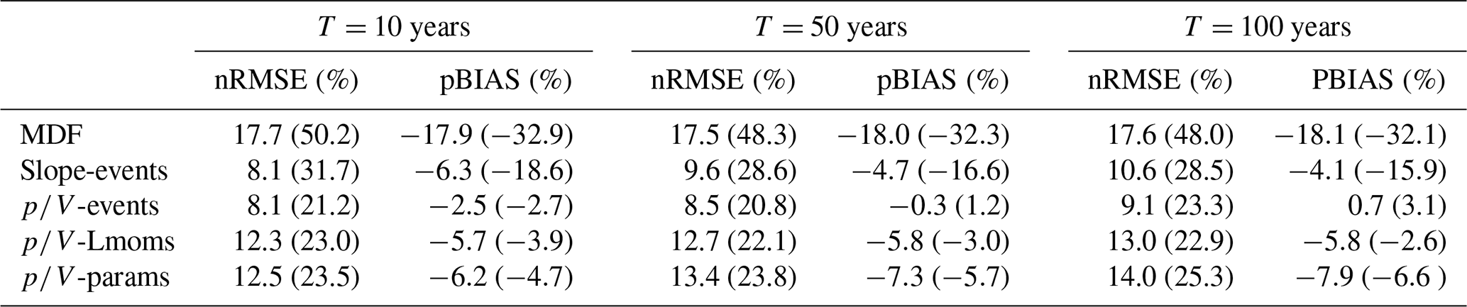
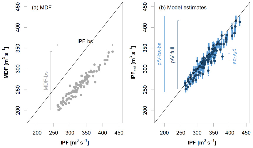
Figure 11 Example of uncertainty ranges with 100 realizations at a single site: (a) HQ100 from IFP-bs vs. MDF-bs, illustrating the sample and parameter uncertainty; (b) HQ100 from IPF_bs vs. estimated IPF, where $p/V$-bs illustrates the $p/V$-Lmoms model uncertainty (shown as dark blue points). $p/V$-full illustrates the propagation of sample and parameter uncertainty through the $p/V$-Lmoms model, and $p/V$-bs-bs illustrates the total uncertainty that combines both sample and parameter uncertainty with the $p/V$-Lmoms model uncertainty.

4.3 Uncertainty analysis

The results of the resampling procedure used to assess uncertainty in the IPF estimates are exemplarily shown in Fig. 11 for the 100-year flood (HQ100) at a single site with a reduced number of 100 realizations. In Fig. 11a, the IPF and MDF estimates for each temporal resampling of the annual maximum series are plotted against each other (IPF-bs and MDF-bs, respectively). This shows the bandwidths of both the IPF and MDF estimates as a result of sample and parameter uncertainty. Figure 11b shows the resampled IPF flood quantiles (IPF-bs) vs. the quantiles estimated using the $p/V$-Lmoms model by considering different sources of uncertainty; $p/V$-bs illustrates the uncertainty only due to the fitting of the $p/V$-Lmoms model, $p/V$-full indicates the sample and parameter uncertainty (MDF-bs) propagated through the $p/V$-Lmoms model, and $p/V$-bs-bs combines the sample and parameter uncertainty (MDF-bs) with the $p/V$-Lmoms model uncertainty ($p/V$-bs) to tackle the total uncertainty. In this example, it becomes obvious that uncertainty from the $p/V$ model ($p/V$-bs) is significantly smaller than the sample and parameter uncertainty (MDF-bs or even IPF-bs). This is valid for the majority of the sites and is hardly affected by the number of realizations.

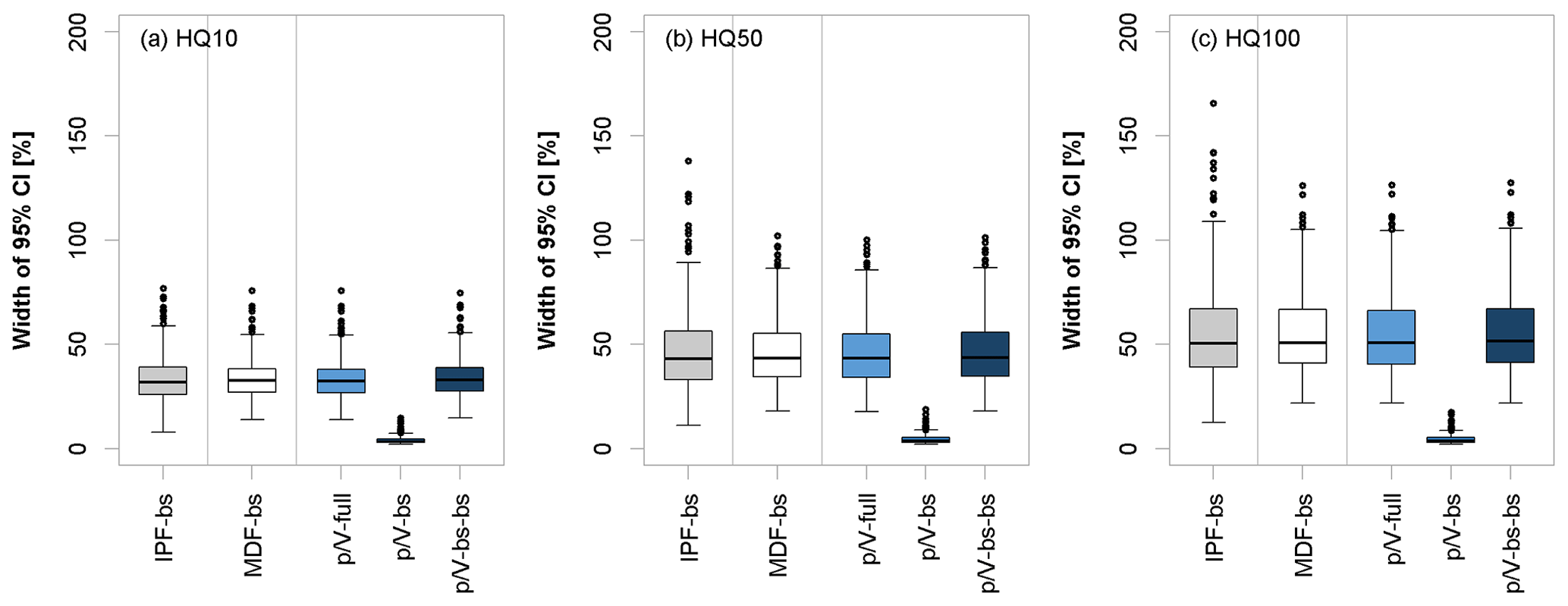
Figure 12 Relative widths of the 95 % confidence interval (as per Eq. 10) of various uncertainty types for different flood quantiles, where IPF-bs and MDF-bs show the sample and parameter uncertainty of the original series, $p/V$-full shows the sample and parameter uncertainty propagated through the $p/V$-Lmoms model, $p/V$-bs shows only the uncertainty of the $p/V$-Lmoms model, and $p/V$-bs-bs shows the total uncertainty that combines both sample and parameter uncertainty with the $p/V$-Lmoms model uncertainty. The boxplots here are obtained for validation sites with more than 30 years of observations.

Figure 12 shows the relative widths of the 95 % confidence intervals for all types of uncertainty estimated. The average widths of the IPF-bs, MDF-bs, and $p/V$-full seem to be similar to each other, where the IPF sample and parameter uncertainty shows greater variability. The width of the average range of the $p/V$-Lmoms model uncertainty ($p/V$-bs) is very small at all the sites and therefore contributes little to the overall level of uncertainty ($p/V$-bs-bs). Thus, the overall uncertainty of the $p/V$-Lmoms model is mainly influenced by the sample and parameter uncertainty of the original MDF series.

In order to assess the full range of the errors in the $p/V$-Lmoms model estimates, they are compared to the range of errors in the MDF estimates. Here, the errors for the uncertainty both in MDF (MDF-bs) and $p/V$-Lmoms ($p/V$-bs-bs) estimates are computed according to Eq. (11). Figure 13 shows the median deviations of the MDF-bs and $p/V$-bs-bs quantiles from the respective IPF-bs quantiles, as well as the lower and upper limits of the 95 % confidence intervals of the errors for the 10-, 50-, and 100-year flood quantiles. The median errors from $p/V$-bs-bs are very similar over the three quantiles, but the higher quantile HQ100 exhibits higher outliers. This is in agreement with the performance of the $p/V$-Lmoms model illustrated in Fig. 9. This means that the median errors obtained over the 1 000 000 realizations are very similar to the actual model errors at each site. Moreover, it is obvious that the overall uncertainty gets larger with increasing return periods, as can be seen by the increasing distance between lower and upper confidence limits. The $p/V$-Lmoms estimates appear to be slightly positively skewed, which is especially noticeable in the 95 % confidence interval for the HQ100. At many of the sites, there is a significant overestimation of the true IPF quantile when combining sample and parameter uncertainty with $p/V$-Lmoms model uncertainty. The MDF estimates, on the other hand, exhibit the expected persistent underestimation.

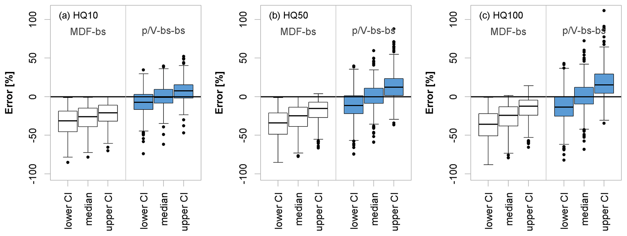
Figure 13 Error distribution obtained as per Eq. (11) for three flood quantiles (a HQ10, b HQ50 and c HQ100 years) from considering the sample and parameter uncertainty of the mean daily flow (MDF) series (MDF-bs in white) and total uncertainty of the $p/V$-Lmoms model ($p/V$-bs-bs in blue). Shown are the median errors as well as the lower and upper limits of the 95 % confidence intervals obtained at the validation sites with more than 30 years of observations.

Figure 14 summarizes the general overlap of the confidence intervals of MDF and estimated IPF with the confidence intervals of the observed IPF for the three flood quantiles (as per Eq. 12). It becomes obvious that the agreement between IPF and the $p/V$-Lmoms model estimates is significantly greater than with the MDF values. This observation suggests that with high probability the $p/V$-Lmoms model estimates are in the range of the “true” IPF quantiles. The fact that overlaps in both the MDF and the models increase with increasing return periods suggests again the overall level of uncertainty in the higher IPF quantiles due to sample and parameter uncertainty.

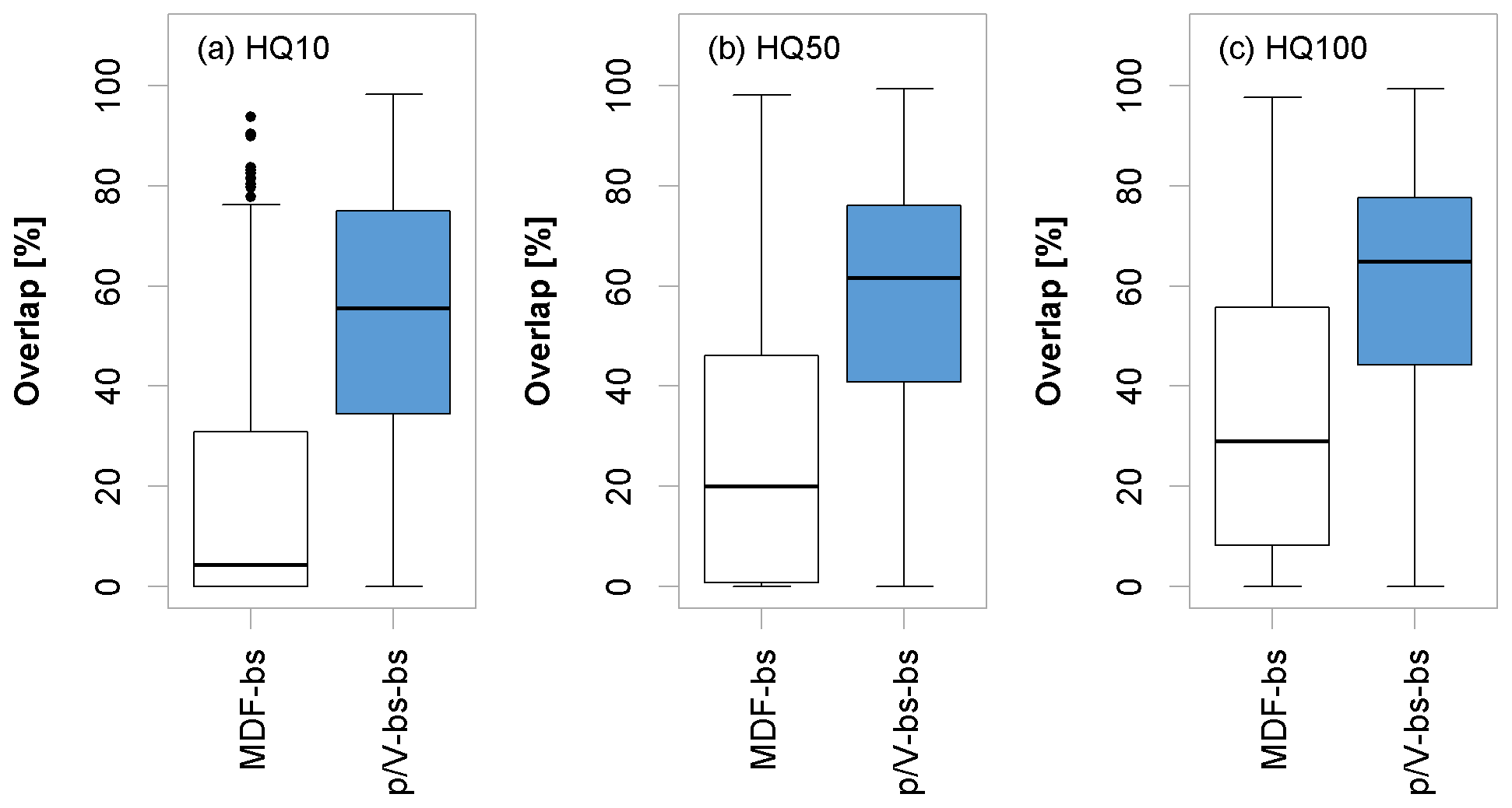
Figure 14 Percentage overlap for the three flood quantiles as per Eq. (12) computed from the 95 % confidence intervals of the MDF sample and parameter uncertainty (MDF-bs) and $p/V$-Lmoms total uncertainty ($p/V$-bs-bs). The boxplots are obtained by considering validation sites with more than 30 years of observations.

5 Discussion

5.1 Factors affecting the correction of MDF to IPF statistics

In theory, the relative deviation between MDF and IPF peaks depends greatly on catchment size, as shown, for instance, in Fuller (1914) and Ellis and Gray (1966). The effect of the catchment size is clearly visible in our data set. The larger the area, the smaller the error between the instantaneous peak and daily flows and, consequently, the respective computed statistics. For catchments smaller than 1000 km², this error can reach down to −80 %. Small catchments without an appreciable buffering capacity react quickly to even low rainfall, leading to short and steep flood waves that are hardly reproduced on coarsely averaged timescales. Factors like steep slopes, impermeable underground, and short but intense rainfall contribute to the flashiness of storm events and make these events less representable through daily flow records. For areas larger than 5000 km², this error becomes very small ($<-\mathrm{20}$ %). This agrees well with the findings of Ellis and Gray (1966) and Chen et al. (2017), which state that, for basins larger than 10 000 km², the peak ratio between MDF and IPF series converges to 1. Larger basins are typically characterized by high baseflow and long response times, which translates to a good representation of IPF from the MDF.

Apart from catchment size, elevation can play also an important role, as shown in Canuti and Moisello (1982). Mountainous catchments have a fast response time and are generally more heavily influenced by meteorological forcing, such as snowmelt processes or convective events, as demonstrated by Gaál et al. (2015). Therefore, the error is expected to increase with high elevation. In our case study, errors at high-altitude sites seem to be particularly significant (40 % to 60 % underestimation). However, this could be a combined effect of small catchments, as mountainous basins are typically smaller in size. On the other hand, sites with elevations lower than 100 m a.s.l. exhibit smaller errors and are stratified according to catchment size. For example, basins larger than 5000 km² show a lower error at an elevation of 100 m compared to 300 m a.s.l. The effect of the elevation on the higher altitudes is less visible in our data set. Apart from the error in the peak magnitude, a weak link is also visible between the high elevation and a smaller temporal overlap between the MDF and IPF peaks.

Different flood genesis, considered here by separating the data into two seasons (winter and summer), also exhibits different error behaviour. Overall, summer IPF statistics were up to 20 % more underestimated than winter IPF statistics. This occurs mainly due to the presence of frequent convective events and moderate rainfall on snow – which enable faster catchment responses. As the summer peaks are underestimated, consequently, when performing a typical annual maximum flow series, summer events will be underrepresented, resulting in a non-representative fitted probability distribution. This is visible in catchments with areas under 500 km², where up to 40 % of annual peaks are falsely chosen from the winter season. Apart from not being able to properly identify flood magnitudes when using mean daily flow, this is a serious issue for the classification of flood regimes, identification of dominating flood types, and application of heterogeneous flood frequency analyses when daily data are the only available options.

Additionally, other factors such as the type and amount of precipitation, soil initial conditions and characteristics, or slope and land use have been shown to influence the on-site variation between instantaneous peak and daily flows. Since their combined effect generates a distinctive daily flow hydrograph, the $p/V$ ratio becomes an important predictor for describing the on-site and between-site variations when correcting MDF events or statistics. The same principle also holds for the slope-method correction suggested by Chen et al. (2017). However, in contrast to the slope method, the $p/V$ ratio contains information about the direct flood volume, which may describe the variability between events and catchments better. This is shown to be the case mainly for catchments under 500 km², where the proposed linear models based on the $p/V$ ratio outperform the slope method. However, this can be attributed to the integration of the most important predictors (such as area, elevation, or $p/V$ ratio) or to the poor performance of the slope methods for areas under 500 km² as discussed in Chen et al. (2017).

5.2 Range of applications and limitations

All the correction methods applied here, either on MDF peak flow events or MDF statistics, generated better agreement with IPF statistics than the statistics from the pure MDF series. The slope methods overall exhibited a constant underestimation around 10 % to 20 % of the IPF statistics. This also agrees with the results from Chen et al. (2017), where a similar underestimation for catchments in Iowa, USA, was also observed. On the other hand, the $p/V$ methods were less biased than the slope method. Although all the $p/V$ models proposed had similar performance, the L-moment method ($p/V$-Lmoms) is more preferable due to its convenience. Correcting the MDF L moments not only ensures a complete correction of the distribution, including both low and high quantiles, but is also not restricted to a type of probability distribution. The method of correcting the error in MDF floods using the $p/V$ ratio performs well and is easily applicable in our study area. However, its great simplification and mere approximation of physical flood-generating processes result in some problems and limitations that will be listed and discussed here.

The first aspect that may influence the performance of the proposed IPF correction method is the event separation technique. The chosen technique determines how flood events and thus the required hydrograph characteristics are defined. The choice of baseflow-separating algorithm can greatly affect the identification of start and end points of flood events. Strict independence criteria and thresholds for event recognition may lead to rejection of crucial flood events when considering daily time series. Lax criteria, on the other hand, may create unnaturally long multi-peak events and false inclusion of small events, leading to unrealistic hydrograph characteristics and IPF estimates. Thus, the additional step of refining multiple peak events, as suggested by Tarasova et al. (2018), should be carried out when rainfall and snowmelt information is available. In their study, the refinement led to a reduction in multi-peak events from more than 50 % to 44.7 % of all identified events. In this study, the ratio of multi-peak to single-peak events is 57.9 % for the year, 58.2 % for summer, and 58.4 % for winter.

Using the $p/V_{\mathrm{event}}$ in order to correct individual events and then using the corrected series for FFA in theory represents a more sensible approach than using the $p/V_{\mathrm{mean}}$ from the annual MDF maxima. As mentioned above, maximum MDF events do not necessarily coincide with maximum IPF events, which is why correcting all events first and then selecting the annual maxima should yield a more appropriate IPF sample. However, again, correcting individual events depends greatly on a very careful event separation, which could not be achieved in this case and which led to some unrealistic IPF estimates. Nonetheless, if a proper event separation is possible, the event correction method may have the greater potential. In such a case, a single model would be sufficient to account for all aspects of IPF estimation, including high flood quantiles.

A problem for IPF correction, which has been exhaustively discussed above, has to do with the gauges that exhibit little difference between MDF and IPF floods, even though their $p/V$ ratio would suggest a much larger error. For our catchments, this applies to the lowest-altitude gauges in the data set. The MDF at these sites are overcorrected and thus exhibit severe overestimation of the true IPF. We therefore discourage the application of the suggested correction methods at catchment outlets situated below 100 m a.s.l.

This observation may also suggest that other factors need to be considered for proper error estimation or that the parameters of the correction models need to be adjusted for different subsets of data. This is also relevant for the question of the universality of the proposed method. Our data set is limited and representative of a temperate humid climate and moderate altitude. Thus, a qualitative sensitivity analysis was carried out on the full 648-site data set in order to identify patterns that could be extrapolated to other regions. The subsets were selected by combinations of geographical location, catchment size, and gauge elevation. The target variable was the mean annual maximum IPF. Differences in the individual models due to different degrees of freedom are natural, which is why only the subsets that lead to significant deviations from the original model are mentioned here.

Two sets of sites deviate noticeably from the original model. The first includes the low-altitude gauges discussed before. Here, the overall error is so small that no correction yields better results than correction via the $p/V$ approach. The second group includes the catchments with areas under 50 km². The errors for these sites appear very scattered and randomly distributed. Comparing the $p/V$ from the daily series with the $p/V$ obtained from instantaneous events, it becomes obvious that the difference increases with decreasing catchment size and becomes excessively large and random for catchment sizes under 100 km². The correction using the mean daily $p/V$ only functions where unknown instantaneous flood dynamics are roughly approximated by observed daily flow variability. The smaller the temporal scale of an instantaneous flood event, the more poorly it is reproduced in the daily records. If instantaneous events manifest themselves primarily on a sub-daily basis, the possibility of describing their dynamics via daily flows becomes ineligible. This observation is also in accordance with the observed temporal shifts between MDF and IPF events, which are increasingly pronounced in smaller catchments. In summary, the proposed correction method flounders at smaller scales below 100 km². Even though the IPF estimation leads to a general improvement at this scale, the daily flood timescale is a poor predictor in these catchments. In other cases, when the flood timescale is larger than 1 d, the $p/V$ predictor should be able to capture the flood dynamics. Still, attention must be paid to the baseflow separation to ensure that the calculated $p/V$ predictor is representative of the catchment behaviour.

On the other hand, for catchments between 100 and 500 km², the $p/V$ models showed the best results. This can be attributed to the selected predictors, whose combination is more representative of these catchments. It can also be attributed to the available data set, as the majority of the sites have a catchment area under 500 km² and the fitted linear models may favour the minimization of the errors for these catchments, although the conducted uncertainty analysis showed that the model uncertainty (due to the selected sites) is very low compared to the local parameter and sample uncertainty.

Nevertheless, the effect of the data set should not be neglected when determining which and how many locations should be grouped together for the fitting of the linear model. Even in the optimal case that the $p/V$ predictor describes the flood dynamics correctly at each site, the question of how well a single linear model can represent the whole group of sites arises. Although L moments are considered more robust than parameters or quantiles, they may differ significantly for a particular group. Hence, a more reasonable approach would be to break the group down into sub-groups. In our case, longitude and latitude did not appear to have any effect on the model fitting. Dividing the study area into quadrants did not result in any differences between the subsets, even when considering a similar catchment size and elevation. Also, neither the record length nor the period of record appeared to have an influence.

The distinction between summer and winter for representation of the two most opposite flood types is particularly valid for this study area and should be adjusted where flood types are otherwise distributed. In general, even the rough distinction between different flood types for IPF estimation proved meaningful in our case, as it revealed different dynamics and MDF–IPF relationships. This observation could be further exploited by more carefully defining and distinguishing between flood types, as e.g. proposed by Fischer (2018) or Tarasova et al. (2018).

Finally, one should note that the type of distribution for flood quantile estimation can only be selected based on daily data and may differ from the optimal IPF distribution. For our data, the GEV proved flexible enough to be a good match for both MDF and IPF, but this could differ in other cases.

6 Conclusions and outlook

As in other studies before this one, it could be shown that the mean daily flow (MDF) and instantaneous peak flow (IPF) relationship depends primarily on the catchment size. It could also be observed that other factors, in this case gauge elevation, play a role in determining the difference between MDF and IPF floods. The relationship also appeared to differ between the two types of floods considered here, i.e. winter and summer floods. Since summer floods are often caused by short but intense rain events and thus exhibit steep rising and falling limbs, their sub-daily peaks are much higher than and difficult to estimate from the smoothed average daily peaks. Long, voluminous winter floods, on the other hand, show a much smaller IPF–MDF ratio and are easier to model.

This study has also shown that hydrograph characteristics, like the peak-to-volume ratio of flood events, can be used to estimate instantaneous peak flows when only average daily series are available. The $p/V$ ratio may be used to predict both the IPF of individual events and instantaneous flood statistics, including mean annual and seasonal maximum flows and flood quantiles. Due to improper flood event separation, the event correction method produced some outliers in our case but may work significantly better when flood events can be defined more carefully. In general, the $p/V$ method requires a minimum of data and can be applied using only information from the daily series itself. The performance could be marginally improved by including gauge elevation as an additional predictor in some of the models.

The general recommendation for estimating IPF flood quantiles is to use the average $p/V$ approach for correction of L moments. This method is convenient, since L moments can be globally corrected, while distributions may be locally fitted afterwards. It turns out that the first two L moments are easily estimated using $p/V_{\mathrm{mean}}$, while higher-order L moments or L-moment ratios are more difficult to model with this approach.

There are two limitations where the proposed method should be handled with care: (a) at sites with elevations below 100 m, since it overestimates the true difference between IPF and MDF; and (b) at catchments smaller than 100 km², where it underestimates the error, so that the full correction potential cannot be achieved. Still, in comparison to the slope method, the $p/V$ approach works significantly better for smaller catchment areas, especially under 500 km². For larger catchments, the slope method appears very robust for all catchment sizes and elevations. The $p/V$ methods perform better in many larger catchments, but outliers may be produced where the above-mentioned restrictions are met. For future analyses, it will be meaningful to test the universality of the proposed approach in other study regions. Also, the effect of the flood event separation on the IPF-estimation performance should be analysed in more detail, especially in order to improve the event correction technique. Finally, it will be interesting to see whether explicit consideration of more carefully defined flood types can improve the IFP estimation in mixed models.