Evaporation and sublimation measurement and modeling of an alpine saline lake influenced by freeze–thaw on the Qinghai–Tibet Plateau

Saline lakes on the Qinghai–Tibet Plateau (QTP) affect the regional climate and water cycle through water loss (E, evaporation under ice-free conditions and sublimation under ice-covered conditions). Due to the observational difficulty over lakes, E and its underlying driving forces are seldom studied when targeting saline lakes on the QTP, particularly during ice-covered periods (ICP). In this study, the E of Qinghai Lake (QHL) and its influencing factors during ice-free periods (IFP) and ICP were first quantified based on 6 years of observations. Subsequently, three models were calibrated and compared in simulating E during the IFP and ICP from 2003 to 2017. The annual E sum of QHL is 768.58±28.73 mm, and the E sum during the ICP reaches 175.22±45.98 mm, accounting for 23 % of the annual E sum. E is mainly controlled by the wind speed, vapor pressure difference, and air pressure during the IFP but is driven by the net radiation, the difference between the air and lake surface temperatures, the wind speed, and the ice coverage during the ICP. The mass transfer model simulates lake E well during the IFP, and the model based on energy achieves a good simulation during the ICP. Moreover, wind speed weakening resulted in an 7.56 % decrease in E during the ICP of 2003–2017. Our results highlight the importance of E in ICP, provide new insights into saline lake E in alpine regions, and can be used as a reference to further improve hydrological models of alpine lakes.

1 Introduction

Saline lakes account for 23 % of the total area and 44 % of the total water volume of Earth's lakes (Wurtsbaugh et al., 2017). They are critical in shaping the regional climate and maintaining ecological security and sustainable development in arid regions (Messager et al., 2016; Wurtsbaugh et al., 2017; Woolway et al., 2020; Wu et al., 2021, 2022). Under the influences of climate change and human activities, saline lakes worldwide have changed rapidly in terms of their area, level, temperature, ice phenology, energy, and water exchange, which have become issues of concern (Gross, 2017; Wurtsbaugh et al., 2017; Woolway et al., 2020). Evaporation under ice-free periods (IFP) and sublimation under ice-covered periods (ICP) are important mechanisms of the transfer of energy and water between lakes and the atmosphere and are among the major factors influencing changes in lake water volume (Ma et al., 2016; Zhu et al., 2016; Woolway et al., 2018, 2020; Guo et al., 2019).

In contrast to freshwater lakes, E (evaporation under IFP and sublimation under ICP) of saline lakes involves a more complex process and is affected not only by climate conditions, lake depth, temperature, stratification, thermal stability, and hydrodynamics, but also by salinity (Salhotra et al., 1985; Hamdani et al., 2018; Obianyo, 2019; Woolway et al., 2020). For example, dissolved salt ions can reduce the free energy of water molecules (i.e., reduce water activity) and result in a reduced saturated vapor pressure above saline lakes at a given water temperature (Salhotra et al., 1987; Mor et al., 2018). Previous studies have investigated the relationship between the E and salinity of saline lakes together with discrepancies in the controlling factors between different timescales (Salhotra et al., 1987; Lensky et al., 2018; Hamdani et al., 2018; Mor et al., 2018). These studies have mainly focused on saline lakes in arid and temperate zones, and the interaction and mutual feedback between the water bodies of saline lakes and the atmosphere remain unclear. There are few studies on the E of alpine saline lakes that exhibit complex hydrology and limnology.

Saline lakes account for over 70 % of the total lake area on the Qinghai–Tibet Plateau (QTP) (Liu et al., 2021) and thus profoundly affect the regional climate and water cycle through the E (Yang et al., 2021). However, continuous year-round direct measurements of saline lake E are scarce, which hinders the exploration of lake E at different timescales. Observations of E from saline lakes have been obtained for Qinghai Lake (QHL) (Li et al., 2016), Nam Co (Wang et al., 2015; Ma et al., 2016), Selin Co (Guo et al., 2016), and Erhai (Liu et al., 2015) via the eddy covariance (EC) technique or pan E on the QTP, but these observations are mainly for the IFP (approximately mid-May to mid-October). Thus, there are considerably fewer E observations during the ICP and full-year period of lakes, mostly because of the harsh environment and limited accessibility to the QTP (Zhu et al., 2016). However, most lakes on the QTP exhibit a long and stable ICP lasting more than 100 d due to the low annual air temperature (T_a) (Cai et al., 2019), which suggests that E observations are currently lacking for nearly a quarter of the year (from the IFP to the ICP). Although studies have commented on the importance of E during the ICP (Li et al., 2016; Wang et al., 2020) and clarified that freezing–breakup processes could result in sudden changes in lake surface properties (such as albedo and roughness) and affect the water and energy exchange between the lake and atmosphere (Cai et al., 2019; Yang et al., 2021), the dynamic processes of energy interchange and the E of saline lakes during the ICP and its responses to climatic variability on the QTP still constitute a knowledge gap in lake hydrology research. Thus, there is an urgent need to better quantify lake E during the ICP on the QTP.

Many models have been employed to calculate lake E, mainly including the Dalton formula series based on mass transfer and aerodynamics, energy and water balance formula series, Penman formula series considering both aerodynamics and the energy balance, and empirical formulas based on statistical analysis (Dalton, 1802; Bowen, 1926; Penman, 1948; Harbeck et al., 1958; Finch and Calver, 2008; Hamdani et al., 2018; Wang et al., 2019a). However, the reported values exhibit large discrepancies in their seasonal variations and annual amounts between those models (Zhu et al., 2016; Ma et al., 2016; Guo et al., 2019; Wang et al., 2019a, 2020), and almost all the models were calibrated and verified against E observations during the IFP, while E during the ICP was either not calculated or was unverified (Wang et al., 2020) as a result of the deficiency in the observed E during the ICP (Zhu et al., 2016; Guo et al., 2019). In addition, compared with small lakes, large and deep lakes exhibit higher E levels and delayed seasonal E peaks because more energy is absorbed and stored in large and deep lakes during the IFP and is released during the ICP (Wang et al., 2019a). Thus, the effect of changes in ice phenology on lake E is particularly important, which calls for different models for E simulation during the IFP and ICP.

Furthermore, with increasing overall surface air warming and moistening, solar dimming, and wind stilling since the beginning of the 1980s (Yang et al., 2014), lakes on the QTP have experienced a significant temperature increase (at a rate of 0.037 ^∘C yr⁻¹ from 2001 to 2015) (Wan et al., 2018) and ice phenology shortening (at a rate of −0.73 d yr⁻¹ from 2001 to 2017) (Cai et al., 2019). Changes in T_a, water surface temperature (T_s), wind speed (WS), and ice phenology could impose different effects on energy interchange and molecular diffusion due to differences in the state phase and reflectance of water between the ICP and IFP, thus altering lake E (Wang et al., 2018). Although many studies have reported a decrease in lake E on the QTP by model simulations (Ma et al., 2016; Zhu et al., 2016; Li et al., 2017; Guo et al., 2019), owing to E neglect during the ICP, the potential mechanisms of lake E and its different responses to climate variability during the ICP and IFP remain unclear.

In this study, based on 6 continuous years of direct measurements of lake E and energy exchange flux data obtained with the EC technique pertaining to QHL, the largest saline lake on the QTP, between 2014 and 2019, we quantified the characteristics of energy interchange and E on diurnal, seasonal (IFP, ICP, and cycle year: AN), and yearly timescales and identified the potential factors influencing E during the IFP and ICP. In addition, combined with reanalysis climate datasets, a mass transfer model (MT model), an atmospheric dynamics model (AD model), and a model based on energy, temperature, and WS (the Jensen–Haise, JH, model) were calibrated and verified, with the optimal model chosen for the simulation of lake E and its response to climatic variability during the IFP and ICP from 2003 to 2017. The results highlight the importance and potential mechanisms of E during the ICP and can be used as a reference to further improve hydrological models of alpine lakes.

2 Materials and methods

2.1 Study area

QHL (36^∘32^′–37^∘15^′ N, 99^∘36^′–100^∘47^′ E; 3194 m a.s.l.), with an area of 4432 km² and a catchment of 29 661 km², is the largest inland saline lake in China (Li et al., 2016). The average depth of the lake is 26 m. The average salt content is 14.13 g L⁻¹, and the pH ranges from 9.15 to 9.30. The hydrochemical type of the lake water is Na–SO₄–Cl (Li et al., 2016). Surrounded by mountains, QHL is a typical closed tectonic depression lake which is fed by five major rivers, i.e., the Buha, Shaliu, Hargai, Quanji, and Heima rivers (Jin et al., 2015). The total annual water discharge is approximately 1.56×10⁹ m³, of which the Buha River contributes 50 % and the Shaliu River contributes approximately one-third (Jin et al., 2015). The mean annual T_a, precipitation, and E values between 1960 and 2015 were −0.1 ^∘C, 355 mm, and 925 mm, respectively (Li et al., 2016). The seasonal stratification of QHL corresponded to that of a dimictic lake, with the spring overturn taking place around May and the fall overturn appearing around November–December (Su et al., 2019). The ICP usually begins in late November, ends in mid–late March or even early April, and lasts approximately 100 d. Under the effects of climate warming, QHL has experienced temperature increases, area expansion, and ICP shortening in the last 2 decades (Tang et al., 2018; Han et al., 2021).

2.2 Site description and energy exchange flux and climate data

The instruments to measure the energy exchange flux and micrometeorological parameters were installed at the Chinese Torpedo Qinghai Lake test base (36^∘35^′27.65^′′ N, 100^∘30^′06^′′ E; 3198 m a.s.l.) located in the southeastern QHL approximately 737 m from the nearest shore (Li et al., 2016) (Fig. 1). The water depth underneath this platform is 18 m. The torpedo test tower has a height of 10 m above the water surface. The EC system was installed on a steel pillar mounted on the northwestern side of the top of the torpedo test tower with a total height of 17.3 m above the lake water surface (Li et al., 2016). A three-dimensional sonic anemometer (model CSAT3, Campbell Scientific Inc., Logan, UT, USA) was used to directly measure horizontal and vertical wind velocity components (u, v, and w) and the virtual temperature. An open-path infrared gas analyzer (model EC150, Campbell Scientific Inc.) was applied to measure fluctuations in water vapor and carbon dioxide concentrations. Fluxes of sensible heat (H) and latent heat (LE) were calculated from the 10 Hz time series at 30 min intervals and were recorded by a data logger (CR3000, Campbell Scientific Inc.). The observation instruments were powered by solar energy.

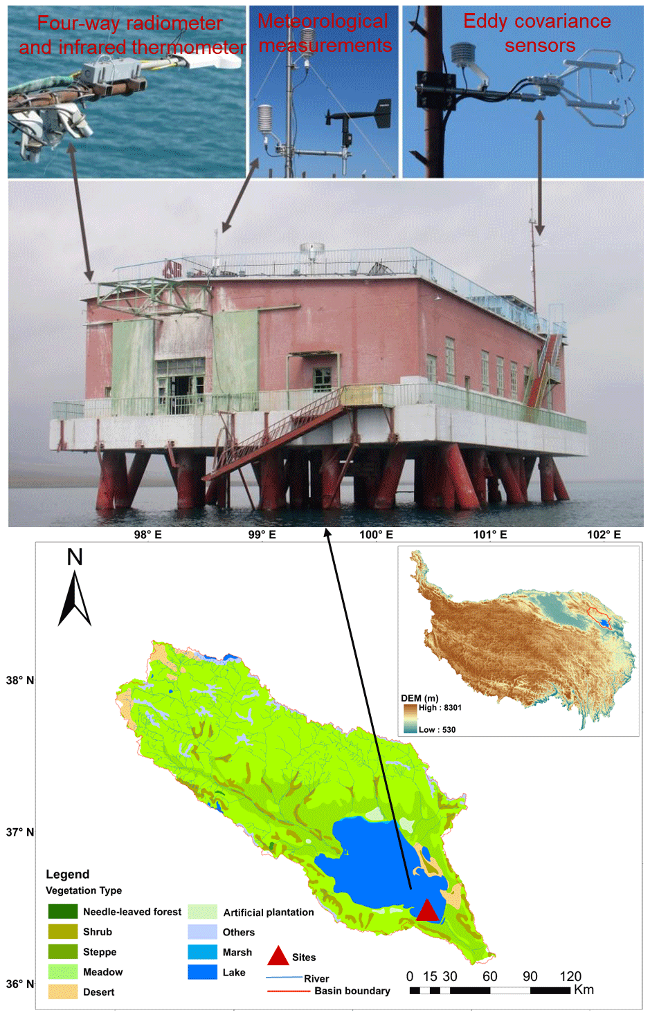
Figure 1 Locations of Qinghai Lake (below) and the measurement site of the Chinese Torpedo Qinghai Lake test base (above). The insets in the uppermost picture are photos of the four-way radiometer and infrared thermometer (left), meteorological variable measurements (middle), and eddy covariance sensors (right). The scale is just for the Qinghai Lake basin.

A suite of auxiliary micrometeorology was also measured as 30 min averages of 1 s readings on the eastern side of the top of the torpedo test tower, 3 m from the EC instruments. The net radiation (R_n) was calculated from the incoming shortwave, reflected shortwave, and incoming and outgoing longwave radiation, which were measured by a net radiometer (CNR4, Kipp & Zonen B.V., Delft, the Netherlands) 10 m above the lake surface (Fig. 1; Table S1 in the Supplement). The T_a, relative humidity (RH), and air pressure (Pres) were measured at a height of 12.5 m above the water surface (Table S1). A wind sentry unit (model 05103, RM Young, Inc., Traverse City, MI, USA) was employed to measure the WS and wind direction (WD) (Table S1). The T_s was measured with an infrared thermometer (model SI-111, Campbell Scientific Inc.) approximately 10 m above the water surface, and the water temperature (T_l) was measured with five temperature probes (109 L, Campbell Scientific Inc.) at depths of 0.2, 0.5, 1.0, 2.0, and 3.0 m. Precipitation was measured with an automated tipping-bucket rain gauge (model TE525, Campbell Scientific Inc.) and a precipitation gauge (model T-200B, Campbell Scientific Inc.) (Table S1). The observation system began operation on 11 May 2013. In this study, we unified all observational data at 30 min intervals and analyzed the data from 1 January 2014 to 31 December 2019 (Table S1).

2.3 Reanalysis climate datasets

The reanalysis climate datasets used to drive the lake E models were acquired from the interim reanalysis dataset v5 (ERA5) produced by the European Centre for Medium-Range Weather Forecasts (https://cds.climate.copernicus.eu/cdsapp#!/search?type=dataset, last access: 6 January 2024) and the China Regional High-Temporal-Resolution Surface Meteorological Elements-Driven Dataset (CMFD) (https://cstr.cn/18406.11.AtmosphericPhysics.tpe.249369.file, last access: 6 January 2024). Gridded hourly ERA5 skin temperature and daily WS, daily CMFD T_a, Pres, RH, and downward shortwave radiation (R_s at a spatial resolution of 0.1^∘ from 2001 to 2018 were analyzed in this study (Table S1). The daily skin temperature was generated by averaging the hourly temperature over 24 h per day and was adopted as the lake surface temperature. We extracted climate data pertaining to QHL via a grid mask with a spatial resolution of 0.1^∘ and averaged the data in all the pixels. Considering the advantages of long time spans and high resolution, the ERA5 and CMFD datasets developed based on land station data have been recognized as the best currently available reanalysis products and have been widely applied in land surface and hydrological modeling studies in China (Ma et al., 2016; Zhu et al., 2016; Tian et al., 2021; Xiao and Cui, 2021). To reduce the uncertainty caused by the input data, the daily lake surface temperature and WS from ERA5, T_a, R_s, RH, and Pres from the CMFD for QHL were adjusted with fitting equations of the observed daily T_s (R²=0.92, P<0.01), WS (R²=0.55, P<0.01), T_a (R²=0.90, P<0.01), R_s (R²=0.73, P<0.01), RH (R²=0.63, P<0.01), and Pres (R²=0.95, P<0.01) from 2014 to 2018 (Fig. S1 in the Supplement), and the equations are shown below.

$$\begin{array}{}\text{(1)}& {\displaystyle }& {\displaystyle }{T}_{\mathrm{a}}^{\mathrm{ad}}=\mathrm{1.01}\times T_{\mathrm{a}}^{\mathrm{CMFD}}+\mathrm{0.71}\text{(2)}& {\displaystyle }& {\displaystyle }{T}_{\mathrm{s}}^{\mathrm{ad}}=\mathrm{0.71}\times T_{\mathrm{s}}^{\mathrm{ERA}\mathrm{5}}+\mathrm{3.30}\text{(3)}& {\displaystyle }& {\displaystyle }{R}_{\mathrm{s}}^{\mathrm{ad}}=\mathrm{0.86}\times R_{\mathrm{s}}^{\mathrm{CMFD}}+\mathrm{34.63}\text{(4)}& {\displaystyle }& {\displaystyle }{\mathrm{WS}}^{\mathrm{ad}}=\mathrm{0.60}\times {\mathrm{WS}}^{\mathrm{ERA}\mathrm{5}}+\mathrm{0.76}\text{(5)}& {\displaystyle }& {\displaystyle }{\mathrm{RH}}^{\mathrm{ad}}=\mathrm{0.68}\times {\mathrm{RH}}^{\mathrm{CMFD}}+\mathrm{19.95}\text{(6)}& {\displaystyle }& {\displaystyle }{\mathrm{Pres}}^{\mathrm{ad}}=\mathrm{0.97}\times {\mathrm{Pres}}^{\mathrm{CMFD}}+\mathrm{30.72}\end{array}$$

$T_{\mathrm{a}}^{\mathrm{ad}}$, $T_{\mathrm{s}}^{\mathrm{ad}}$, $R_{\mathrm{s}}^{\mathrm{ad}}$, WS^ad, RH^ad, and Pres^ad are the T_a, T_s, R_s, WS, RH, and Pres, respectively, of ERA5 and CMFD after adjustment.

2.4 Lake ice coverage dataset and ice phenology

The daily lake ice coverage of QHL from 2002 to 2018 was extracted from a lake ice coverage dataset of 308 lakes (with an area greater than 3 km²) on the QTP retrieved from the National Tibetan Plateau Data Center (Qiu et al., 2019). The dataset with a time span from 2002 to 2018 was generated from the Moderate Resolution Imaging Spectroradiometer (MODIS) normalized difference snow index (NDSI, with a spatial resolution of 500 m) product with the SNOWMAP algorithm, and the data under cloud cover conditions were redetermined based on the temporal and spatial continuity of lake surface conditions (Qiu et al., 2019). Based on the lake ice coverage, the IFP was defined as having ice coverage lower than 10 %, and the ICP was defined as having ice coverage higher than 10 % (Qiu et al., 2019). The ICP was divided into three stages: freeze (FZ: 10 % < ice coverage < 90 %), complete freeze (CF: ice coverage > 90 %), and thaw (TW: 10 % < ice coverage < 90 %) (Qiu et al., 2019). We defined the cycle year (annual: AN) from the beginning of the IFP to the end of the ICP. This ice coverage has been compared with that from two other datasets based on passive microwaves and was found to be highly consistent with the others at an average R² of 0.86 and a root mean square error (RMSE) of 0.13 in QHL (Qiu et al., 2019). Thus, this dataset is very accurate and suitable for the division of lake ice phenology in QHL.

2.5 Data processing of the observed energy exchange flux and climate data

The EC fluxes were processed and corrected based on the 10 Hz raw time series data in the data processing software EdiRe, including spike removal, lag correction of water to carbon dioxide relative to the vertical wind component, sonic virtual temperature correction, performance of planar fit coordinate rotation, density fluctuation correction (WPL correction), and frequency response correction (Li et al., 2016). Since the shortest distance between the Chinese torpedo Qinghai Lake test base and the southwestern lakeshore is only 737 m, there may be insufficient fetch for a turbulent flux under certain conditions. Therefore, footprint analysis was conducted to eliminate data influenced by the surrounding land. For further details on the process and results of the footprint analysis, see Li et al. (2016). In addition to these processing steps, quality control of the 30 min flux data was conducted using a five-step procedure: (i) data originating from periods of sensor malfunction were rejected (e.g., when there was a faulty diagnostic signal), (ii) data within 1 h before or after precipitation were rejected, (iii) incomplete 30 min data were rejected when the missing data constituted more than 3 % of the 30 min raw record, (iv) data were rejected at night when the friction velocity was below 0.1 m s⁻¹ (Blanken et al., 1998), and (v) data with large footprints (>700 m) and a wind direction from 180 to 245^∘ were eliminated.

To further control the quality of the energy exchange flux (sensible heat flux and latent heat flux: H and LE, respectively) and micrometeorological dataset (R_n, T_a, T_s, T_l, RH, WS, Pres, and albedo), data outside the mean ± 3 × standard deviation were removed for each variable. Then, gap-filling methods entailing a look-up table and mean diurnal variation (Falge et al., 2001) were adopted to fill gaps in the flux measurement data. The look-up table method was applied when the meteorological dataset was available synchronously. Otherwise, the mean diurnal variation method was adopted. The heat storage change (G, W m⁻²) was estimated as a residual of the energy balance:

$$\begin{array}{}\text{(7)}& G=R_{\mathrm{n}}-\mathrm{LE}-H,\end{array}$$

where R_n is the net radiation (W m⁻²), H is the sensible heat flux (W m⁻²), and LE is the latent heat flux (W m⁻²). Lake E was calculated as

$$\begin{array}{}\text{(8)}& E=\mathrm{LE}÷\mathit{\lambda },\end{array}$$

where λ is the latent heat of vaporization (MJ kg⁻¹), taken as 2.45 MJ kg⁻¹ in this paper (Allen et al., 1998).

2.6 Models for daily lake evaporation simulation

To evaluate the interannual variation in QHL E from 2003 to 2017, we validated three models during the AN, IFP, and ICP. Qinghai Lake is a saline lake, and many studies have pointed out that it is worth considering the influence of salinity on saline lake evaporation. With the increase in salinity, it will exert a greater inhibition on evaporation (Hamdani et al., 2018; Mor et al., 2018). Thus, the water activity coefficient (α), which is defined as the ratio between the vapor pressure above saline water and that above freshwater at the same temperature, has been introduced to characterize the effect of salinity on saline lake evaporation (Salhotra et al., 1987; Lensky et al., 2018). Because saline water drains out salt during freezing (Badawy, 2016), we only introduced the α into the evaporation simulation of Qinghai Lake during IFP. The three models were as follows.

1. MT model (Harbeck et al., 1958)

   $$\begin{array}{}\text{(9)}& {\displaystyle }& {\displaystyle }{E}_{\mathrm{MT}}=N\times F\left(\mathrm{WS}\right)\times \mathrm{\Delta }e\text{(10)}& {\displaystyle }& {\displaystyle }F\left(\mathrm{WS}\right)=a\mathrm{1}\times \mathrm{WS}+a_{\mathrm{2}}\text{(11)}& {\displaystyle }& {\displaystyle }\mathrm{\Delta }e=\left\{\begin{array}{ll}\mathit{\alpha }\times e_{\mathrm{s}}-\mathrm{RH}\times e_{\mathrm{a}}& \mathrm{during}\mathrm{IFP}\\ e_{\mathrm{s}}-\mathrm{RH}\times e_{\mathrm{a}}& \mathrm{during}\mathrm{ICP}\end{array}\right.\text{(12)}& {\displaystyle }& {\displaystyle }{e}_{\mathrm{s}}=\mathrm{6.105}\times \exp \left({\displaystyle \frac{\mathrm{17.27}\times T_{\mathrm{s}}}{T_{\mathrm{s}}+\mathrm{237.7}}}\right)\text{(13)}& {\displaystyle }& {\displaystyle }{e}_{\mathrm{a}}=\mathrm{6.105}\times \exp \left({\displaystyle \frac{\mathrm{17.27}\times T_{\mathrm{a}}}{T_{\mathrm{a}}+\mathrm{237.7}}}\right)\end{array}$$

   E_MT is the E rate (mm d⁻¹), N is the mass transfer coefficient, WS is the wind speed (m s⁻¹), Δe is the vapor pressure difference, RH is the relative humidity, and e_s and e_a are the saturated vapor pressures at the lake surface temperature (T_s) and air temperature (T_a), respectively. An α value of 0.97 was suggested for QHL during IFP, as measured with a portable water activity meter (AwTester, China). This model inherently accounts for the water salinity through Δe and requires calibration of coefficients N, a₁, and a₂, which were taken to be 1.26, 0.04, and 0.17 during the AN, respectively; 0.41, 0.17, and 0.28 during the IFP, respectively; and 0.90, 0.18, and 0.28 during the ICP, respectively, in this study.

2. AD model (Hamdani et al., 2018)

   $$\begin{array}{}\text{(14)}& {\displaystyle }& {\displaystyle }{E}_{\mathrm{AD}}={\displaystyle \frac{\mathrm{0.622}\times C_{\mathrm{e}}}{{\mathit{\rho }}_{\mathrm{w}}\times P}}\times {\mathit{\rho }}_{\mathrm{a}}\times \mathrm{WS}\times \mathrm{3.6}\times {\mathrm{10}}^{\mathrm{6}}\times \mathrm{\Delta }e\text{(15)}& {\displaystyle }& {\displaystyle }{\mathit{\rho }}_{\mathrm{a}}=\mathrm{1.293}\times \left({\displaystyle \frac{\mathrm{273.15}}{\mathrm{273.15}+T_{\mathrm{a}}}}\right)\times {\displaystyle \frac{\mathrm{Pres}}{\mathrm{101.325}}}\end{array}$$

   ρ_w and ρ_a denote the water and air densities (kg m⁻³), respectively, and ρ_w is approximately 1.011×10³ kg m⁻³ for QHL. Moreover, Pres is the air pressure (mbar), and C_e is a transport coefficient obtained via calibration to address missing friction velocity values in the reanalysis climate datasets and taken to be $\mathrm{4.10}\times {\mathrm{10}}^{-\mathrm{3}}$, $\mathrm{3.80}\times {\mathrm{10}}^{-\mathrm{3}}$, and $\mathrm{8.40}\times {\mathrm{10}}^{-\mathrm{3}}$ during the AN, IFP, and ICP, respectively, in this paper.

3. Statistical model based on solar radiation (JH model) (Wang et al., 2019b)

   $$\begin{array}{}\text{(16)}& E_{\mathrm{JH}}={\mathrm{JH}}_{\mathrm{1}}\times \left({\mathrm{JH}}_{\mathrm{2}}\times \left(T_{\mathrm{a}}-T_{\mathrm{s}}\right)+{\mathrm{JH}}_{\mathrm{3}}\right)\times \left(R_{\mathrm{s}}\right)\times \left(\mathrm{WS}\right)\end{array}$$

   R_s is the incoming solar shortwave radiation (W m⁻²); JH₁, JH₂, and JH₃ must be calibrated and were taken to be 0.06, $-\mathrm{2.20}\times {\mathrm{10}}^{-\mathrm{3}}$, and $\mathrm{5.03}\times {\mathrm{10}}^{-\mathrm{3}}$ during the AN, respectively; 0.08, $-\mathrm{2.00}\times {\mathrm{10}}^{-\mathrm{3}}$, and 0.04 during the IFP, respectively; and 0.02, $\mathrm{7.40}\times {\mathrm{10}}^{-\mathrm{3}}$, and 0.18 during the ICP, respectively, in this paper.

The three models were selected, first, as they are typical representatives in considering mass transfer, aerodynamics, and energy transfer; second, because their demand parameters are easy to acquire and are adaptive to being promoted; and third, as they have been proven to be efficient in saline lakes (Hamdani et al., 2018). These models were first calibrated and validated based on daily E observations from 2014 to 2019 during AN, IFP, and ICP, respectively. The RMSE and goodness of fit (R²) were used to evaluate the effectiveness of the models. A model with high R² and low RMSE values was selected for lake E simulation during the AN, IFP, and ICP.

2.7 Statistical analysis

Summer and fall were taken as June to August and September to November, respectively. During data analysis, we first divided the 30 min observed energy exchange flux and climate data from 2014 to 2019 by the AN, IFP, and ICP based on the calculated ice phenology. Hence, we obtained datasets of 5 cycle years from the IFP in 2014 to the ICP in 2018 (Fig. S2). Second, we calculated the multiday average 30 min energy exchange flux during the IFP and ICP in each year to evaluate the basic statistical characteristics of the diurnal E and exchange flux. The daily energy exchange flux and climate data were calculated by averaging the 30 min observed data for each day, and the daytime (nighttime) energy exchange flux and climate data were calculated by averaging the 30 min observed data of 08:00 to 19:30 LT (20:00 to 07:30 LT). One-way ANOVA was performed to compare the difference in E and G between the IFP and ICP in each year from 2014 to 2018. Third, to explore the key factor controlling lake E, partial least squares regression and random forest methods were used to calculate the sensitivity coefficient (representing the regression coefficient of each variable, which means the amount of change in E caused by the variation per unit in the variable) and importance of R_n, WS, Δe, Pres, albedo, WD, T_a−T_s, T_l, and ICR to E during the daytime and nighttime of IFP and ICP, respectively. The two methods analyze the relationship between E and climate and environmental factors from linear and nonlinear processes, respectively, and have been widely used in the study of hydrological and ecological fields (Desai and Ouarda, 2021; Li et al., 2022; Sow et al., 2022). Finally, three models were validated and two models were selected to separately calculate the interannual E during the IFP and ICP from 2003 to 2017 (the available ice phenology exhibits a limited cycle year from 2003 to 2017). Four controlled tests were then conducted to quantify the contribution of the variation in T_a, T_s, WS, and R_s to lake E from 2003 to 2017. The analysis of partial least squares regression, random forest methods, and E simulation, calibration, and verification was conducted with daily datasets. The partial least squares and random forest analyses were conducted in R, and the others were conducted in MATLAB.

3 Results

3.1 Diurnal and seasonal characteristics of evaporation and the energy budget during the different freeze–thaw periods

The average E, LE, G, H, and R_n values (average from 2014 to 2018) were 1.20±0.09 mm d⁻¹, 68.01±4.93 W m⁻², 192.18±7.00 W m⁻², 16.25±1.21 W m⁻², and 276.45±3.32 W m⁻², respectively, during the IFP; and 1.11±0.20 mm d⁻¹, 63.15±11.31 W m⁻², 79.23±18.12 W m⁻², 4.68±0.37 W m⁻², and 147.06±14.23 W m⁻², respectively, during the ICP. The daytime E, LE, G, H, and R_n values were notably lower during the ICP than during the IFP, except for E and LE in 2014 (Figs. 2 and 3; Table S2). In addition, the daily peak LE and E values typically occurred at approximately 12:00 LT during the IFP and at approximately 14:00 LT during the ICP and exhibited an approximately 2 h lag during the IFP and a 4 h lag during the ICP over G and R_n (Fig. 2). At night, although lower E (at an average rate of 0.81±0.17 mm d⁻¹) and LE (46.02±9.71 W m⁻²) levels occurred during the ICP than during the IFP (at average rates of 0.94±0.05 mm d⁻¹ and 53.09±2.94 W m⁻², respectively), E (LE) accounted for 42 %–45 % and 41 %–45 % of the total daily E during the IFP and ICP, respectively (Figs. 2 and 3; Table S2). Regarding G, a similar release rate was found during the IFP and ICP, but the heat release time was longer during the ICP than during the IFP (Fig. 2).

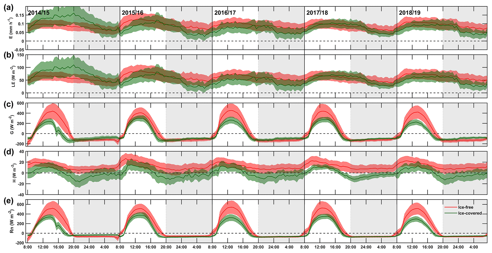
Figure 2 Diurnal characteristics of evaporation (E), latent heat flux (LE), sensible heat flux (H), heat storage change (G), and net radiation (R_n) of Qinghai Lake (QHL) during the ice-free and ice-covered periods (IFP and ICP) from 2014 to 2018. The multiday average 30 min data during the IFP and ICP in each cycle year are shown here, and the colored shading indicates 0.5 SD (standard deviation). The gray area indicates nighttime. The labels 2014/2015, 2015/2016, 2016/2017, 2017/2018, and 2018/2019 indicate the cycle years of the freeze–thaw cycles.

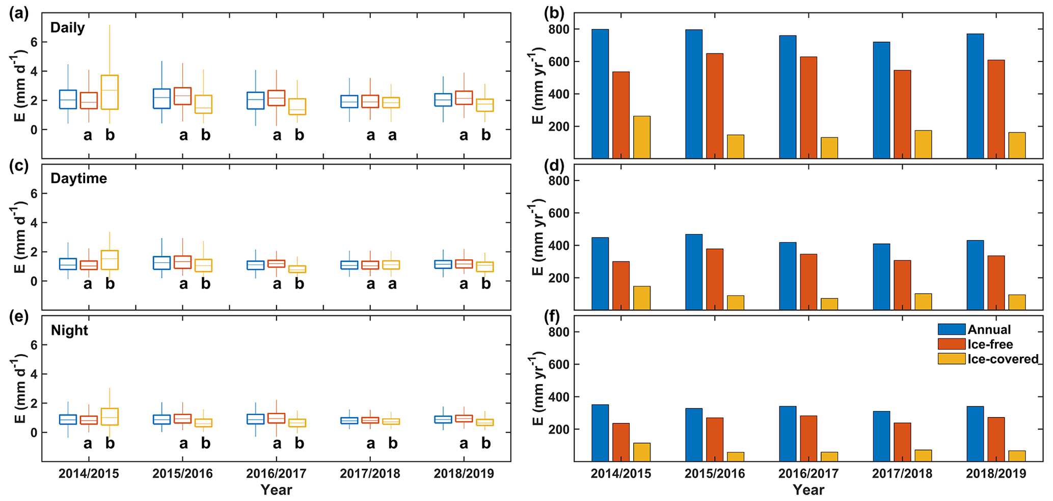
Figure 3 E rate (a, c, e) and annual E sum (b, d, f) of QHL during the cycle year (annual: AN) and IFP and ICP in each cycle year from 2014 to 2018. Panels (a) and (b) show daily data, panels (c) and (d) show daytime data, and panels (e) and (f) show nighttime data. The whiskers in panels (a), (c), and (e) show the 1.5 interquartile range, while the letter associated with the whiskers indicates statistically significant differences via one-way ANOVA during the different freeze–thaw periods in each year from 2014 to 2018. The labels 2014/2015, 2015/2016, 2016/2017, 2017/2018, and 2018/2019 indicate the cycle year of freeze–thaw cycling.

The daily E ranged from 1.96 to 2.34 mm d⁻¹ during the IFP and from 1.57 to 2.71 mm d⁻¹ during the ICP, and the average E sum reached 593.37±44.87 mm yr⁻¹ during the IFP and 175.22±45.98 mm yr⁻¹ during the ICP from 2014 to 2018 (Figs. 3 and S2; Table S2). This suggested average E sums of 77 % during the IFP and 23 % during the ICP throughout the cycle year from 2014 to 2018 (with a lake E sum ranging from 719.45 to 798.55 mm yr⁻¹ and an average value of 768.58±28.73 mm yr⁻¹) (Fig. 3). In terms of G, QHL initially released heat in fall, which lasted until the lake was completely frozen, after which heat was absorbed from the lake thawing period throughout the summer (Figs. S2 and S3).

3.2 Response of evaporation to climatic factors during the different freeze–thaw periods

The key controlling factor of lake E was explored based on the daily observed energy exchange flux and climate data (E, R_n, WS, Δe, Pres, albedo, WD, T_a−T_s, and T_l) and ICR during the IFP and ICP from 2014 to 2018. The Δe (with sensitivity coefficients of 0.28 in the daytime and 0.22 in the nighttime, P<0.05), WS (with sensitivity coefficients of 0.54 in the daytime and 0.43 in the nighttime, P<0.05) and Pres (with sensitivity coefficients of 0.26 in the daytime and 0.14 in the nighttime, P<0.05) notably increased E (Fig. 4), and the effect was greater in the daytime than in the nighttime during the IFP (Fig. 4). The R_n (with a sensitivity coefficient of 0.25 in the nighttime, P<0.05), WS (with sensitivity coefficients of 0.30 in the daytime and 0.22 in the nighttime, P<0.05), T_a−T_s (with sensitivity coefficients of 0.59 in the daytime and 0.39 in the nighttime, P<0.05), and ICR (with sensitivity coefficients of 0.20 in the daytime and 0.17 in the nighttime, P<0.05) imposed a significant positive effect on E during the ICP (Fig. 4). Similarly, the top five important factors calculated with the random forest method were WS, Δe, Pres, WD, and T_s during the IFP and T_a−T_s, T_a, WS, R_n, and ICR during the ICP (Fig. S4). This indicated that E of QHL was mainly controlled by WS, Δe, and Pres during the IFP but was driven by R_n, T_a−T_s, WS, and ICR during the ICP.

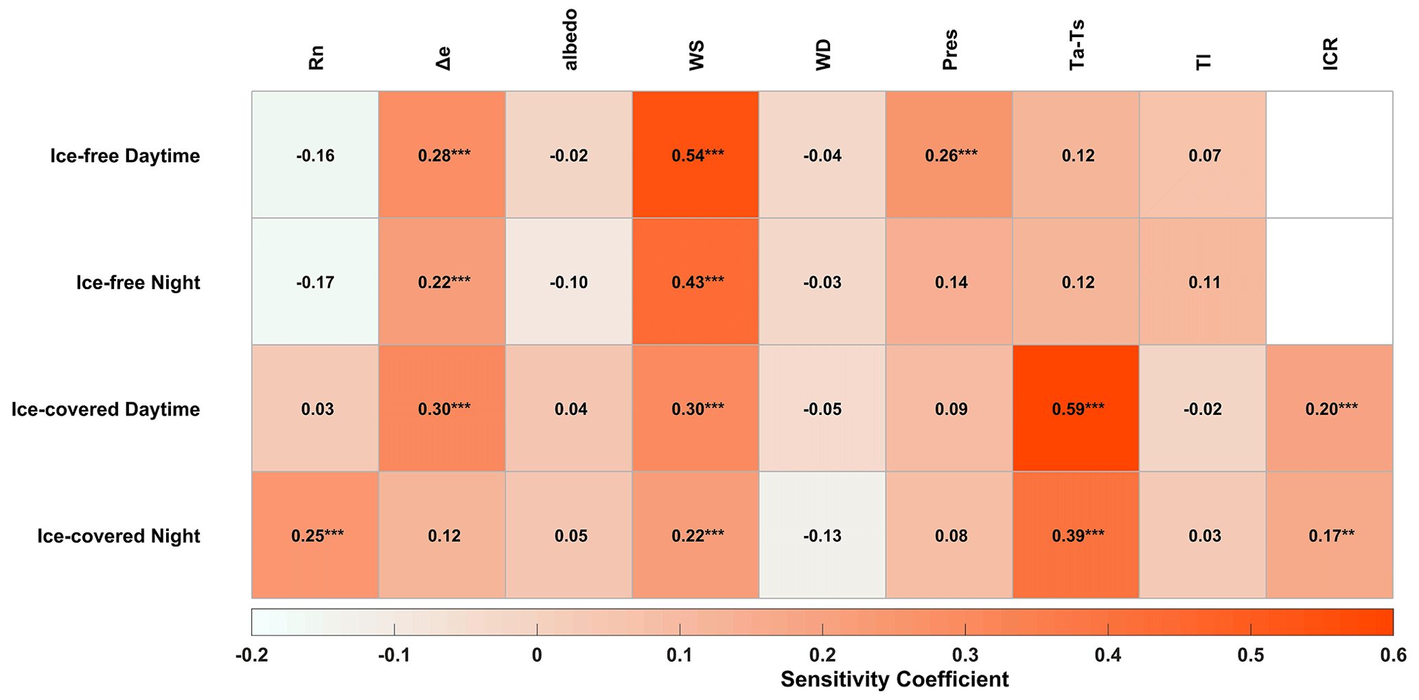
Figure 4 Sensitivity coefficient between the daytime and nighttime climatic factors and the E rate of QHL during IFP and ICP. ^*, ${}^{**}$, and ${}^{***}$ indicate statistical significance at the P<0.1, P<0.05, and P<0.01 levels, respectively, via Student's t tests. R_n, Δe, WS, WD, Pres, T_a−T_s, T_l, and ICR indicate the net radiation, vapor pressure difference, wind speed, wind direction, pressure, difference between the air and lake surface temperatures, average temperature of the lake body from 0 to 300 cm, and ice coverage rate, respectively.

3.3 Evaporation simulation and interannual variation

Three models (MT, AD, and JH) were calibrated and validated to evaluate the interannual variation in QHL E from 2003 to 2017. In the case of model performance, the MT model based on molecular diffusion performed the best in terms of E simulation during the IFP (with the largest R² and smallest RMSE values of 0.79 and 0.85, respectively), while the JH model based on energy exchange performed the best during the ICP (with the largest R² and smallest RMSE values of 0.65 and 1.02, respectively) (Figs. S5 and S6). Thus, the interannual variation in E from 2003 to 2017 was calculated with the MT model during the IFP and with the JH model during the ICP (Fig. 5). From 2003 to 2017, increases in Δe (at a rate of 0.01 hPa yr⁻¹) and T_s (at a rate of 0.001 ^∘C yr⁻¹) resulted in an increase in E (at a rate of 1.62 mm yr⁻¹ for the E sum) during the IFP (Figs. 5 and S7). Conversely, ignoring the increases in T_a (at a rate of 0.04 ^∘C yr⁻¹) and T_a−T_s (at a rate of 0.04 ^∘C yr⁻¹), with decreasing WS (at a rate of −0.005 m s⁻¹ yr⁻¹), E (at a rate of −1.98 mm yr⁻¹ for the E sum) decreased during the ICP, which resulted in an inapparent decrease in E (at a rate of −0.36 mm yr⁻¹ for the E sum) during the AN (Figs. 5 and S7).

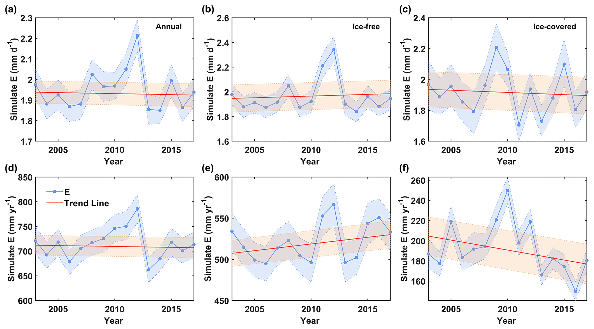
Figure 5 Interannual variability in the simulated E rate (a–c) and annual E sum (d–f) of QHL in AN, IFP, and ICP from 2003 to 2017. The blue shading indicates 0.5 SD, and the red shading indicates the 95 % confidence interval of the trend line.

4 Discussion

4.1 Lake evaporation during the ice-covered period

The results of this study highlight the important contribution of lake ice sublimation to the total amount of lake E. Due to the low snow coverage of Qinghai Lake in winter (with a maximal snow coverage of less than 16 % of the area of Qinghai Lake), evaporation and sublimation of lake ice and water are the major sources of E during the ICP of 2013–2018 (Fig. S8). The experimental and simulation results of Jambon-Puillet et al. (2018) verified that the E rates of liquid droplets and ice crystals remain the same under unchanged environmental conditions. In this study, the E rate of QHL during the ICP ranged from 1.57 to 2.71 mm d⁻¹, approximately 0.73–1.38 times that of liquid water during the IFP (Table S2), with similar results to those findings of liquid droplets and ice crystals. Few studies have examined lake ice E during the ICP, most of which have focused on polar sea ice and alpine snowpacks (Froyland et al., 2010; Froyland, 2013; Herrero and Polo, 2016; Christner et al., 2017; Lin et al., 2020). Observational and modeling studies of Antarctic ice sheets or lakes have found that the monthly E rate of ice ranged from −4.6 to 13 mm per month from June to September (Antarctic) (Froyland et al., 2010). In this study, we found that the E sum ranges from 130.59 to 262.45 mm during the ICP (approximately 51.60 to 81.3 mm per month, by multiplying the mean daily E of ICP by 30) from 2014 to 2018, which is higher than the previous observations from Antarctic ice sheets or lakes. This may be because Antarctic ice sheets or lakes are located at high latitudes with low solar radiation and are therefore cooler from the surface to greater depths with energy-limiting conditions for E (Persson et al., 2002). However, the lakes on the QTP freeze seasonally, and most of these lakes can store a large amount of heat because of the high solar radiation during the IFP (Fig. 6), which leads to the observed E during the ICP (Huang et al., 2011, 2016). Studies on surface E of a shallow thermokarst lake in the central QTP region have found that E reaches up to 250 mm yr⁻¹ during the ICP (Huang et al., 2016), which is close to our observed E levels (130.59–262.45 mm yr⁻¹). Our results further showed that E of QHL accounted for 23 % of the annual E during the ICP. Wang et al. (2020) evaluated 75 large lakes on the QTP and demonstrated that the E of these lakes in winter accounted for 12.3 %–23.5 % of the annual E, which suggests that E of these lakes during the ICP was the same as that during the other seasons. Furthermore, considering that the area of QHL is 4432 km² (Li et al., 2016), QHL releases 3.39±0.13 km³ of water into the air every year, which corresponds to the sum of the water for animal husbandry, industrial, and domestic uses in Qinghai Province (an average of 2014 to 2017) (Dong et al., 2021).

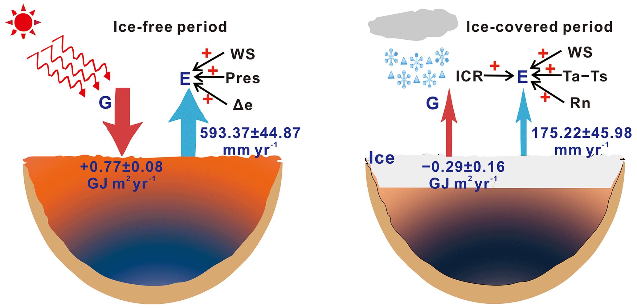
Figure 6 E and G in QHL during IFP and ICP. WS, Pres, Δe, T_a−T_s, R_n, and ICR are the wind speed, air pressure, vapor pressure difference, difference between T_a and T_s, net radiation, and ice coverage rate of the lake, respectively. The red plus sign indicates a positive effect of the variable on E.

4.2 Responses of lake evaporation to salinity

Salinity greatly influences the E of saline lakes by changing both water density and thermal properties; dissolved salt ions can reduce the free energy of water molecules and result in a higher boiling point and reduced saturated vapor pressure above saline lakes (Salhotra et al., 1987; Abdelrady, 2013; Mor et al., 2018). Therefore, an increase in the salinity of a lake would decrease its E rate. For example, Houk (1927) compared the E of pure water with that of saline lakes of different densities (salinity) in Nevada, USA, and found that, when the density (salinity) of water increased by 1 %, the E of saline lakes decreased by 0.01 % compared with that of pure water. Similarly, Mor et al. (2018) found that the E rate in the diluted plume is nearly 3 times larger than that in an open lake in the Dead Sea. Thus, the thermodynamic concept of water activity which is defined as the ratio of water vapor pressure on the surface of saline water and freshwater at the same temperature (the water activity of freshwater is 1, while that of saline water is lower than 1, and the higher the salinity is, the lower the water activity in lakes is) has been widely used in E simulations of saline lakes (Salhotra et al., 1987; Abdelrady, 2013; Mor et al., 2018). In our study, we measured the water activity of QHL as 0.97 by a salinity of 14.13 g L⁻¹ and applied it to the MT and AD models for E simulation of IFP during 2003 to 2017, which makes it more theoretical to explain the E process of saline lakes and reduces the uncertainty of estimation in saline lake E. For example, with the salinity of 133 g L⁻¹ of surface water, water activity was measured to be 0.65 and has been widely used in its E simulation of the Dead Sea (Metzger et al., 2018; Mor et al., 2018; Lensky et al., 2018), and Abdelrady (2013) improved the surface energy balance system (SEBS) of E in saline lakes by constructing an exponential function between lake salinity and water activity, which reduced the simulated E by 27 % and the RMSE from 0.62 to 0.24 mm (3 h)⁻¹ in Great Salt Lake. Therefore, considering salinity is essential for enhancing the accuracy of E simulations in saline lakes.

4.3 Responses of lake evaporation to climate variability

In addition, climate and environment are also important factors affecting lake E and vary significantly between the different seasons. Previous studies have shown that lake E is mostly affected by WS and Δe in summer and by WS, Δe, T_a−T_s, and G in winter (Zhang and Liu, 2014; Hamdani et al., 2018). This suggests that energy exchange between lakes and air may be one of the main drivers of E during the ICP under the same atmospheric boundary conditions (Fig. 6). Since most lakes store heat in summer, they release heat and sufficiently produce E in winter (Blanken et al., 2011; Hamdani et al., 2018). In this study, we also found that QHL began to store heat in the lake thawing period and released heat in fall or when the lake began to freeze (Figs. 6 and S3). Therefore, E of QHL was mostly controlled by WS, Δe, and Pres during the IFP, whereas it was mainly affected by R_n, T_a−T_s, and WS during the ICP (Fig. 6).

Furthermore, the QTP has been suffering surface air warming and moistening, solar dimming, and wind stilling since the beginning of the 1980s (Yang et al., 2014; Kuang and Jiao, 2016), which affects the hydrothermal processes of the lake, such as increasing T_s and shortening lake ice phenology (Wan et al., 2018; Cai et al., 2019). An increase in T_s enhances the diffusion of water molecules and enlarges Δe between the water surface and the air, which in turn promotes evaporation (Wang et al., 2018; Woolway et al., 2020), while a reduction in solar radiation decreases the energy input of the lake and wind stilling enhances the stability of the atmosphere above the water surface, which in turn inhibits evaporation (Roderick and Farquhar, 2022; Guo et al., 2019). We found a decrease in E during the AN from 2003 to 2017 due to the steeper decrease in E caused by solar dimming and wind stilling during the ICP than the increase engendered by the increase in T_s during the IFP. From 2003 to 2017, E decreased at average rates of $-\mathrm{6.48}\pm \mathrm{4.77}$ mm yr⁻¹ (3.23 %) and $-\mathrm{1.17}\pm \mathrm{14.291}$ mm yr⁻¹ (7.56 %) due to decreases in R_s and WS, respectively, during the ICP (Fig. 7; Table S3), while the increase in T_s increased E at an average rate of 13.58±20.75 mm yr⁻¹ (3.54 %) during the IFP (Fig. 7; Table S3). Previous studies have found similar results in Selin Co and Namu Co (Zhu et al., 2016; Guo et al., 2019). For example, Guo et al. (2019) found that E was mainly controlled by WS, and a decrease in WS led to a decrease in E from 1985 to 2016 in Selin Co.

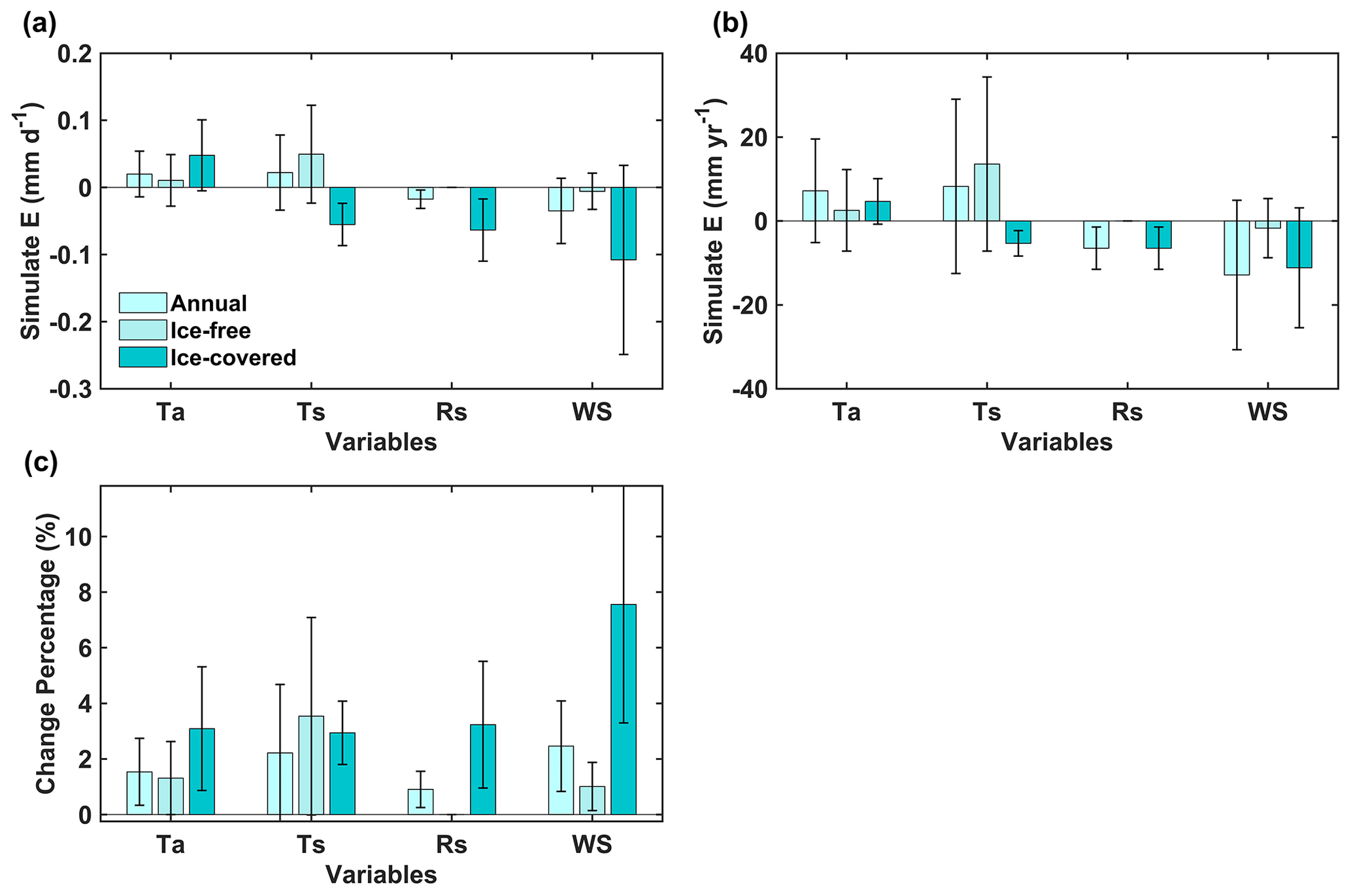
Figure 7 The multiyear average contributions of the changes in air temperature (T_a), lake surface temperature (T_s), downward shortwave radiation (R_s), and wind speed (WS) to the simulated E of QHL in the AN, IFP, and ICP from 2003 to 2017. Panel (a) shows the multiyear average change in the E rate caused by T_a, T_s, R_s, and WS; panel (b) shows the multiyear average change in the annual E sum caused by T_a, T_s, R_s, and WS; and panel (c) shows the multiyear average change percentage of E caused by T_a, T_s, R_s, and WS. The whiskers indicate 0.5 SD.

In addition, changes in lake ice phenology significantly affected lake E during the IFP and ICP. Compared with 2003 to 2007 (101.40±7.00 d), the average ICP decreased by 10.8 d from 2013 to 2017 (90.60±6.08 d) (Table S3). A shortened ICP suggests a much lower albedo in the cycle year and could result in higher R_s absorption and a shorter period for heat-induced recession, which could increase lake E (Wang et al., 2018). Furthermore, lake E is also affected by the lake area, water level, and physical and chemical properties (Woolway et al., 2020), especially for saline lakes (Salhotra et al., 1987; Mohammed and Tarboton, 2012; Mor et al., 2018). Increasing the water salinity could reduce E (Salhotra et al., 1987; Mor et al., 2018) because the dissolved salt ions could reduce the free energy of water molecules (i.e., reduced water activity) and result in a lower saturated vapor pressure above saline lakes at a given water temperature (Salhotra et al., 1987; Mor et al., 2018). However, the changes in lake physical and chemical properties attributed to lake freezing increase the complexity of the underlying mechanism, simulation of ice E, and its response to climate change, and more studies are needed to further explore interactions between the different factors.

4.4 Limitation

Based on six continuous year-round direct measurements of lake E and energy exchange flux, we determined the E loss during the ICP and calibrated and verified different models for E simulation during the IFP and ICP. Due to the lack of accurate measurements of deep lake temperatures, energy budget closure ratios of EC observations in QHL are not given in this study. EC measurements have been widely used to quantify the E of several global lakes, including Lake Superior in North America, Great Slave Lake in Canada, Lake Geneva in Switzerland, Lake Valkea–Kotinen in Finland, and Taihu Lake, Erhai Lake, Poyang Lake, Nam Co, Selin Co, and Ngoring Lake in China (Blanken et al., 2000, 2011; Vercauteren et al., 2009; Nordbo et al., 2011; Wang et al., 2014; Li et al., 2015, 2016; Liu et al., 2015; Guo et al., 2016; Ma et al., 2016; Lensky et al., 2018). With most of the known energy budget closure ratios over 0.7, EC observations of lakes are regarded as an accurate and reliable direct measurement method of E, even in lakes over the QTP (Wang et al., 2020). Moreover, compared with land stations, the energy budget closure ratios over lake surfaces can be significantly influenced by the large amount of heat storage (release) during different seasons (Wang et al., 2020), which would increase the uncertainty about the quantification of E. In addition, quantification of E during the ICP depends on accurate ice phenology identification, and a longer ICP suggests more E. Therefore, the different data sources and phenological classification methods of ice phenology comprise one source of uncertainty. Moreover, lake salinity changes dynamically at diurnal, seasonal, and interannual scales, but due to the difficulty in continuously observing lake salinity, the fixed water activity in our study may cause the underestimation in E of QHL due to the decrease in salinity by the expansion of QHL. Furthermore, in addition to the traditional lake evaporation models (Dalton formula series, energy and water balance formula series, Penman formula series, and empirical formula based on statistical analysis), the one-dimensional lake thermodynamics model has been widely used for the simulation of lake ice thickness and energy balance (ice sublimation) in ICP (Pour et al., 2017; Stepanenko et al., 2019; Xie et al., 2023). Considering that this study concentrated on verifying the consistency of the accuracy of the traditional models for the evaporation simulation during IFP and ICP, it ignored the one-dimensional lake thermodynamics model for ice sublimation. It is suggested to build the observation system of lake thermodynamic parameters and to verify and develop suitable one-dimensional or even three-dimensional lake thermodynamic evaporation models for QHL in future studies.

5 Conclusions

In summary, based on six continuous year-round 30 min direct flux measurements throughout the cycle year from 2014 to 2018, the night E of QHL occupied over 40 % during both the IFP and ICP. With a multiyear average of 175.22±45.98 mm yr⁻¹, E during the ICP accounted for 23 % of the total cycle year E sum, which is an important component in calculating the E of saline lakes. A difference-based control factor of E was also found during the IFP and ICP. E of QHL was mainly controlled by atmospheric dynamic factors (WS, Δe, and P) during the IFP, whereas it was driven by both energy exchange and atmospheric boundary conditions (R_n, T_a−T_s, and WS) during the ICP. Thus, the MT model based on molecular diffusion performed best in lake E simulation during the IFP, while the JH model based on energy exchange performed best during the ICP. Furthermore, simulation of the E of QHL showed a slight decrease from 2003 to 2017 caused by a decrease in E during the ICP, and WS weakening may have resulted in an average reduction of 7.56 % in lake E during the ICP from 2003 to 2017. Our results suggest that E during the ICP is non-negligible for saline lake E, and E simulation should be further improved in future model simulation studies considering the difference in its potential mechanisms during the ICP.