Identification of parameter importance for benzene transport in the unsaturated zone using global sensitivity analysis

One of the greatest threats to groundwater is contamination from fuel derivatives. Benzene, a highly mobile and toxic fuel derivative, can easily reach groundwater from fuel sources and lead to extensive groundwater contamination and drinking water disqualification. Modelling benzene transport in the unsaturated zone can quantify the risk for groundwater contamination and provide needed remediation strategies. Yet, characterization of the problem is often complicated, due to typical soil heterogeneity, numerous unknown site and solute parameters, and the difficulty of distinguishing important from non-important parameters. Thus, sensitivity analysis (SA) methods, such as global SA (GSA), are applied to reduce uncertainty and detect key parameters for groundwater contamination and remediation. Nevertheless, studies devoted to identifying the parameters that determine transport of fuel derivatives in the unsaturated zone are scarce. In this study, we performed GSA to assess benzene transport in the unsaturated zone. First, a simple GSA (Morris) screening method was used for a homogenous sandy vadose zone. Then, a more computationally demanding (Sobol) variance-based GSA was run on the most influential parameters. Finally, the Morris method was tested for a heterogeneous medium containing clay layers. To overcome model crashes during GSA, several methods were tested for imputation of missing data. The GSA results indicate that benzene degradation rate (λ_k) is the utmost influential parameter controlling benzene mobility, followed by aquifer depth (z). The adsorption coefficient (K_d) and the van Genuchten n parameter of the sandy soil (n₁) were also highly influential. The study emphasizes the significance of λ_k and the presence of clay layers in predicting aquifer contamination. The study also indicates the importance of heterogenous media representation in the GSA. Though identical parameters control the transport in the different soil types, in the presence of both sand and clay, parameters directly affecting the solute concentration like λ_k and K_d have increased influence in clay, whereas n is more influential for sand comprising most of the profile. Overall, GSA is demonstrated here as an important tool for the analysis of transport models. The results also show that in higher dimensionality models, the radial basis function (RBF) is an efficient surrogate model for missing data imputation.

1 Introduction

Petroleum products such as petrol and diesel are among the most abundant chemicals of ecological concern used nowadays. During petroleum exploration, production, transport, and storage, petroleum products often find their way to the environment by accidental leaks and spills (Logeshwaran et al., 2018; López et al., 2008; Nadim et al., 2000). Consequently, groundwater is often polluted by surface sources, posing a substantial potential risk to potable water worldwide (López et al., 2008; Nadim et al., 2000; Logeshwaran et al., 2018; Reshef and Gal, 2017; Kessler, 2022). Since petroleum substances in general, and fuel components in particular, are considered toxic, carcinogenic, and mutagenic (Logeshwaran et al., 2018), strict regulations limit their maximum allowed concentration in groundwater to the parts-per-billion level (U.S. EPA, 2018).

Fuel products are usually comprised of different types of hydrocarbons. Fuel compounds like benzene are among the most commonly found groundwater pollutants (Schmidt et al., 2004; Logeshwaran et al., 2018). Specifically, benzene is highly soluble and thus one of the most mobile fuel constituents in the subsurface (Farhadian et al., 2008). In the US alone, about 9×10⁵ kg was reported to be released into the terrestrial and aquatic environment by the petroleum industries between 1987 and 1993 (Fan et al., 2014). In Israel, benzene was detected in 60 % of all sites monitored for fuel contamination (Reshef and Gal, 2017). Benzene's low maximum acceptable concentration of 5 µg L⁻¹ in drinking water (Farhadian et al., 2008; Kessler, 2022) raises great concerns that benzene leakages into groundwater may disqualify extremely large volumes of drinking water. Most fuel-related contamination reaches groundwater from or near the soil surface (Troldborg et al., 2009). Therefore, it is important to assess the risk to groundwater from soil contamination and to understand the fate and transport of fuel components travelling from the soil surface, through the unsaturated zone, and down to the groundwater.

Since actual water flow and contaminant transport in the subsurface are difficult to measure and predict, mathematical models are used to solve such transport problems (Bear and Cheng, 2010). Many studies have been performed to examine the fate and transport of petroleum hydrocarbons, and specifically of benzene, mostly in saturated homogeneous porous media (Lu et al., 1999; Brauner and Widdowson, 2001; Choi et al., 2005, 2009). Few studies have also assessed the movement of benzene in unsaturated porous media (Berlin et al., 2016; Berlin and Suresh, 2019; Troldborg et al., 2009; Ciriello et al., 2017). Benzene transport models typically combine Darcy-type water flow; advective–dispersive transport; and a source/sink term considering various physical, chemical, and biological processes including sorption, dissolution, and biodegradation (Mohamed and Sherif, 2010). Yet, the typical heterogeneity of the subsurface environment and the difficulty in obtaining sufficient relevant physical and bio-geochemical characterizations of the site lead to high uncertainty of these parameters (Ciriello et al., 2017; Tartakovsky, 2007). Soil heterogeneity and layering, for example, have been shown to considerably affect contaminant transport in some studies (Rivett et al., 2011; Chen et al., 2019), while in others their effect seemed negligible (Botros et al., 2012; Akbariyeh et al., 2018). This of course depends on the model scale, type of system (natural or irrigated), and type of contaminant tested. Also, soil and contaminants' parameters can be estimated using various methods, such as laboratory measurements, scaling, and inverse modelling (Botros et al., 2012; Akbariyeh et al., 2018; Berlin et al., 2016; Berlin and Suresh, 2019; Troldborg et al., 2009; Ciriello et al., 2017). This adds another aspect of uncertainty to the model. Thus, sensitivity analysis (SA) is required to determine the contribution of the individual input parameter to the uncertainty of the model output (Song et al., 2015). More specifically, SA can determine which are the non-influential input parameters that are redundant or can be fixed and reveal the order of parameter importance and the magnitude of parameter interactions (Razavi et al., 2021).

Various SA methods are available; they can generally be classified as local sensitivity analysis (LSA) or global sensitivity analysis (GSA) methods. LSA methods are mostly “one-at-a-time” (OAT) methods (Saltelli and Annoni, 2010; Razavi et al., 2021). These methods are based on changing the uncertain input parameter by a specific interval several times around a “local point” in the problem space (Saltelli and Annoni, 2010; Razavi et al., 2021). The difference or the derivative of the output compared with the base-case output is then tested. LSA methods are usually simple and efficient in analysing simple models, but they are less suitable for multiple-parameter, non-linear, and non-additive models. This is because derivatives are informative at the base point where they are computed but do not enable exploration of the rest of the input parameter space (Saltelli and Annoni, 2010). Moreover, OAT methods are efficient in finding the most influential input parameters but cannot rank the influence of the input parameters or measure parameter interactions (Saltelli and Annoni, 2010). In GSA, on the other hand, the input parameters are changed over the entire sampling space, and the variance or probability distribution of the output is tested rather than the derivative. Variance-based GSA methods are most commonly used since they are conceptually simple and easy to implement (Upreti et al., 2020; Khorashadi Zadeh et al., 2017; Jaxa-Rozen et al., 2021; Saltelli et al., 2010, 2004; Sobol, 2001; Song et al., 2015; Nossent et al., 2011; Brunetti et al., 2016, 2017). Yet, when the model output is highly skewed or multi-modal, the variance may not adequately represent output uncertainty (Liu et al., 2006; Borgonovo, 2007). Therefore alternative methods, such as moment-independent (Liu et al., 2006; Borgonovo, 2007) and moment-based (Dell'Oca et al., 2017) methods, were developed using the output probability density function (PDF) to fully characterize the output uncertainty. In some studies, PDF methods were shown to perform better for ranking the importance of parameters, and though highly influential parameters were usually common, the ranking of these parameters was similar (Wang and Solomatine, 2019; Upreti et al., 2020; Khorashadi Zadeh et al., 2017), and in some cases variance-based methods were preferred (Upreti et al., 2020). In addition to finding the most influential input parameters, GSA can rank the parameters' influence and their interactions (Saltelli and Annoni, 2010; Razavi et al., 2021). Yet, the main drawback of GSA methods is their computational cost.

Most hydrological models have numerous parameters resulting in high-dimensional and non-linear problems. Therefore GSA methods are usually recommended in hydrological modelling (Song et al., 2015). Song et al. (2015) recommended GSA application before final modelling to better understand the model and its dominating parameters and as a tool to reduce the model parametric dimensionality. In their review, Song et al. (2015) identified three main “hot spots” in GSA application with hydrological modelling, that are relevant to many other disciplines. The three hot spots are as follows:

1. Computational cost and subsequent meta-modelling are used instead of running the models multiple times, where the reliability and goodness of fit of meta-models should be explored.

2. Selecting an appropriate GSA method, monitoring the convergence, and estimating the uncertainty of the GSA results are important for hydrological models.

3. GSA methods involve many hypotheses or have other limitations, including the independence of input variables, where in practice, the parameters employed by hydrological models usually have interactions or correlations that need to be considered.

So far, LSA/GSA has rarely been applied for contaminant transport in the unsaturated zone (Davis et al., 1994; Gatel et al., 2019; Gribb et al., 2002; Pan et al., 2011; Rockhold, 2018; Ciriello et al., 2017), where most studies have considered a homogenous media. Specifically for benzene, few local sensitivity analyses have indicated the degradation and adsorption coefficients as the most important parameters for benzene transport in the unsaturated zone (Gribb et al., 2002; Zanello et al., 2021). In one GSA performed to assess the risk of benzene contamination of groundwater (Ciriello et al., 2017), the porosity and hydraulic conductivity of the media were found to be the dominant parameters for the model uncertainty. Yet in that study, properties related to benzene itself (such as its degradation rate or adsorption coefficient) were treated as deterministic quantities and were not tested by the GSA (Ciriello et al., 2017). Moreover, we are not aware of any SA performed for benzene transport in layered heterogenous unsaturated media. Hence, more research is needed to understand the key parameters controlling contaminant transport in the subsurface in general, and for benzene, in particular, to improve prediction and mitigation of groundwater contamination.

The objective of this study was to assess the specific impact of each of the multiple parameters that affect benzene transport in the unsaturated zone. For that purpose, a mechanistic model was used to simulate the transport of benzene in an unsaturated zone representing Israel's coastal plain vadose zone. Simulations of both homogenous (sand) and heterogeneous (sand with clay layers) vadose zones were conducted. Two GSA methods were tested for the homogenous media simulations, to analyse the parameter importance: the Morris method (Morris, 1991), a reliable, computationally cheap alternative to variance-based GSA, and the Sobol method (Sobol, 2001), a computationally heavy and variance-based method and probably the most well-established and widely applied type of GSA (Khorashadi Zadeh et al., 2017; Jaxa-Rozen et al., 2021; Saltelli et al., 2010, 2004; Sobol, 2001; Song et al., 2015; Nossent et al., 2011; Brunetti et al., 2016, 2017, and many more) (see Sect. 2.3 for a description of these methods). The heterogeneous media simulation was tested by the Morris method, where the effect of the parameters of both soil types was tested as well as the clay layers' distribution.

A common though usually overlooked problem in GSA application is that some of the model runs do not converge but crash due to numerical instability and the assignment of random sets of parameters of different values (Razavi et al., 2021; Sheikholeslami et al., 2019). Owing to the novelty of GSA in hydrological research, there is not one agreed and established way to deal with these missing data, and the information in the literature is still scarce (Sheikholeslami et al., 2019). Consequently, and as part of the overall analysis done in this study, we tested several methods for missing data imputation in cases where the model does not converge or crashes.

2 Materials and methods

A mechanistic model was generated to investigate the potential transport of benzene in the vadose zone underlain by Israel's coastal plain aquifer. The model was applied for both homogenous and heterogeneous media. For simplicity, initial runs solely included a homogenous sandy soil profile, as sand and sandstone are the main constituents of Israel's coastal plain aquifer (Kurkar Group; Turkeltauub, 2011). Yet, in most natural environments, the soil profile is non-homogenous, containing clay layers and other materials. In a study conducted in Israel's coastal plain vadose zone, Rimon et al. (2007) reported that the occurrence of different soil materials, and specifically clay interbeds, strongly affects flow patterns to the aquifer. Therefore, later model runs included clay interbeds.

2.1 Mechanistic model and input parameters

The one-dimensional mechanistic model included water flow, solute transport, biodegradation, adsorption, and volatilization. Water flow in the unsaturated zone was modelled by a modified form of Richard's one-dimensional equation:

$$\begin{array}{}\text{(1)}& {\displaystyle \frac{\partial \mathit{\theta }}{\partial t}}={\displaystyle \frac{\partial }{\partial z}}\left[K\left({\displaystyle \frac{\partial h}{\partial z}}+\mathrm{1}\right)\right],\end{array}$$

where h is the water matric head [L], θ is the volumetric water content, t is time [T], z is the vertical coordinate [L] (positive upward), and K is the unsaturated hydraulic conductivity function [L T⁻¹] given by

$$\begin{array}{}\text{(2)}& K(h,z)=K_{\mathrm{s}}\left(z\right)K_{\mathrm{r}}(h,z),\end{array}$$

where K_r is the relative hydraulic conductivity [–] and K_s the saturated hydraulic conductivity [L T⁻¹].

Table 1 Constant input parameters for the model.

The unsaturated soil hydraulic properties θ(h) and K(h) are described by the van Genuchten–Mualem formulation (Mualem, 1976; van Genuchten, 1980):

$$\begin{array}{}\text{(3)}& {\displaystyle }& {\displaystyle }\mathit{\theta }\left(h\right)={\mathit{\theta }}_{\mathrm{r}}+{\displaystyle \frac{{\mathit{\theta }}_{\mathrm{s}}-{\mathit{\theta }}_{\mathrm{r}}}{[\mathrm{1}+\mathrm{|}|\mathit{\alpha }h\mathrm{|}{|}^n{]}^m}}h<\mathrm{0}\text{(4)}& {\displaystyle }& {\displaystyle }K\left(h\right)=K_{\mathrm{s}}{S}_{\mathrm{e}}^l{\left[\mathrm{1}-{\left(\mathrm{1}-S_{\mathrm{e}}^{\mathrm{1}/m}\right)}^m\right]}^{\mathrm{2}}\text{(5)}& {\displaystyle }& {\displaystyle }{S}_{\mathrm{e}}={\displaystyle \frac{\mathit{\theta }-{\mathit{\theta }}_{\mathrm{r}}}{{\mathit{\theta }}_{\mathrm{s}}-{\mathit{\theta }}_{\mathrm{r}}}},\end{array}$$

where

$$\begin{array}{}\text{(6)}& m=\mathrm{1}-\mathrm{1}/n,n>\mathrm{1}.\end{array}$$

In Eqs. (3)–(6), θ_s is the saturated water content and θ_r is the residual water content. α [L⁻¹], n, and m are the van Genuchten fitting parameters; S_e is the effective saturation, and l is the pore-connectivity parameter (Eq. 4).

Solute transport was described by the advection–dispersion equation:

$$\begin{array}{}\text{(7)}& \begin{array}{rl}{\displaystyle \frac{\partial \mathit{\theta }c}{\partial t}}+\mathit{\rho }{\displaystyle \frac{\partial s}{\partial t}}+{\displaystyle \frac{\partial a_{\mathrm{v}}g}{\partial t}}=& {\displaystyle \frac{\partial }{\partial z}}\left(\mathit{\theta }{D}^{\mathrm{w}}{\displaystyle \frac{\partial c}{\partial z}}\right)+{\displaystyle \frac{\partial }{\partial z}}\left(a_{\mathrm{v}}{\mathit{\tau }}_{\mathrm{g}}{D}^{\mathrm{g}}{\displaystyle \frac{\partial g}{\partial z}}\right)\\ & -{\displaystyle \frac{\partial qc}{\partial z}}-{\mathit{\lambda }}_k\mathit{\theta },\end{array}\end{array}$$

where c, s, and g are solute concentrations in the liquid [M L⁻³], solid [MM⁻¹], and gaseous [M L⁻³] phases, respectively. ρ [M L⁻³] is the solid-phase bulk density. D^w is the dispersion coefficient in the liquid phase [L² T⁻¹] given by Bear (1972) as

$$\begin{array}{}\text{(8)}& \mathit{\theta }{D}^{\mathrm{w}}={\mathit{\alpha }}_{\mathrm{L}}q+\mathit{\theta }{D}^{\mathrm{M}}{\mathit{\tau }}_{\mathrm{w}},\end{array}$$

where D^M is benzene's molecular diffusion coefficient in the aqueous phase [L² T⁻¹], q is the absolute value of the Darcian fluid flux [L T⁻¹] evaluated using the Darcy–Buckingham law, and $q=-K\left(\frac{\mathrm{d}h}{\mathrm{d}z}+\mathrm{1}\right)$. α_L is the longitudinal dispersivity [L], and τ_w and τ_g are tortuosity factors in the liquid and gas phase, respectively [–], evaluated using the relationship described by Millington and Quirk (1961). a_v is the air content [L³ L⁻³], D^g is the benzene molecular diffusion coefficient [L² T⁻¹] in the gas phase, and λ_k is a first-order rate biodegradation constant for benzene in the liquid phase [T⁻¹] (solid- and gas-phase degradation was assumed negligible).

Benzene adsorption was assumed linear (Wołowiec and Malina, 2015; Baek et al., 2003) of the form s=K_dc, where K_d is the distribution coefficient [L³ M⁻¹] (see Table S2 in the Supplement for literature values).

The gaseous-phase (g) and aqueous-phase (c) concentrations in Eq. (7) are related by a linear expression of the following form:

$$\begin{array}{}\text{(9)}& g=k_{\mathrm{g}}c,\end{array}$$

where k_g is an empirical constant [–] equal to (K_HR_uT^A)⁻¹ (Stumm and Morgan, 1981), in which K_H is Henry's law constant [M T² M⁻¹ L⁻²], R_u is the universal gas constant [M L² T⁻² K⁻¹ M⁻¹], and T^A is the absolute temperature [K].

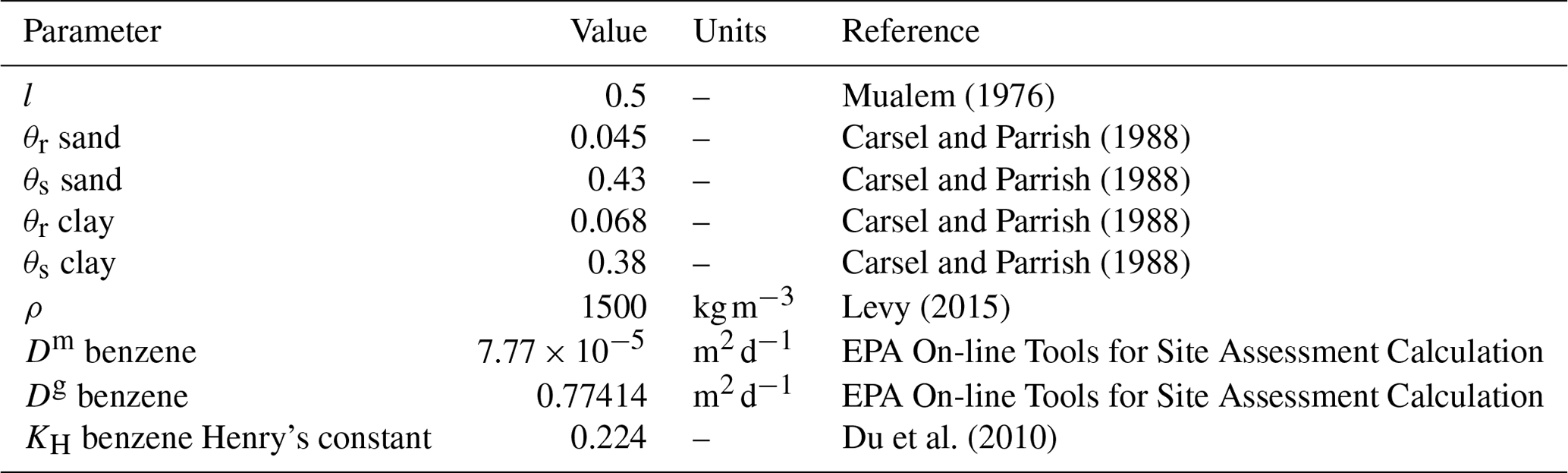
The values of θ_s, θ_r, l, D^M, D^g, K_H, and ρ were kept constant in the model and are listed in Table 1. D^M, D^g, and K_H are constant properties for benzene and were therefore not changed. The pore-connectivity parameter l in the hydraulic conductivity function was estimated to be about 0.5 as an average for many types of soils (Mualem, 1976). The range of θ_s, θ_r, and ρ values in the literature was limited (Carsel and Parrish, 1988; Domenico and Schwartz, 1990; Gribb et al., 2002; Schaap et al., 2001). In a local sensitivity analysis of benzene transport in the vadose zone, Gribb et al. (2002) found that ρ is an insignificant parameter, and θ_r is only significant in pure clayey soils.

Table 2 Input parameters and their range used for GSA.

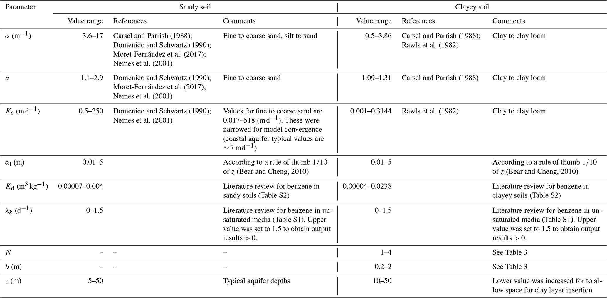
The sensitivity of the model to the values of α, n, K_s, α_L, λ_k, and K_d was tested in the GSA. The range of tested values along with the corresponding references can be found in Table 2. Specifically, we found that λ_k values greatly vary between different studies, mainly due to the differences in experimental conditions and aquifer characteristics (see Table S1 in the Supplement for literature values). Though the highest λ_k value we encountered in the literature was 174 (d⁻¹) (Lahvis et al., (1999); Table S1), we set the upper limit of λ_k to 1.5 (d⁻¹) (Table 2). This was done for two main reasons:

• a.

  From an early stage it was evident that λ_k is a very influential parameter and high values mostly resulted in output values of zero, thereby lowering the overall sensitivity.

• b.

  The Morris analysis takes the range and divides it into a given number of levels (four or six, in our case). Since the range of λ_k included values spanning over 4 orders of magnitude (1 × 10⁻²–1 × 10² (d⁻¹)), much of the range would have been missed by the analysis.

2.2 Model domain and boundary conditions

The profile depth (z) was set as a variable input parameter in the range of 5–50 m (Table 2). This range was obtained from a dataset of fuel-contaminated sites of Israel's coastal plain (see Fig. S1 in the Supplement) from Israel's Ministry of Environmental Protection and reported by Israel's Water Authority (Reshef and Gal, 2017). In runs that tested the occurrence of clay layers, the thickness (b) and number (N) of clay layers were additionally tested as variable GSA input parameters (Table 2).

An upper atmospheric boundary condition (BC) was set at the top of the profile with average daily precipitation and potential evaporation data from the Beit Dagan meteorological station for 2019 (Fig. 1). Potential pan evaporation data were converted to Penman–Monteith potential evaporation by multiplying the data by monthly coefficients obtained for the Israeli coastal plain (Gal et al., 2012). On days when evaporation data were not available, a monthly averaged evaporation value of the available data for the specific month was used as input. At the bottom boundary, where the aquifer was positioned, a Dirichlet BC of constant matric head (h=0) was set.

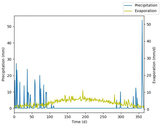
Figure 1 Daily precipitation and potential evaporation data of Beit Dagan meteorological station for 2019 – set as the upper BC of the model.

For the first 10 years, only water flow was considered, to enable stabilization of the hydraulic conditions in the profile and establish annual periodic conditions. According to our tests, stabilization takes about 4 years. Hence, benzene was introduced following 10 years.

For the solute transport, an upper Dirichlet BC prescribing benzene saturation concentration (1.77 kg m⁻³ – solubility of benzene in water at 25 °C; Stewart, 2010) was set to mimic a constant fuel lens on the surface. A bottom Neumann BC of zero concentration gradient was set, enabling free drainage to the aquifer.

The model was run using the Hydrus-1D software package (Šimùnek et al., 2013), a finite element model for simulating the one-dimensional movement of water and solutes in variably saturated media. In the homogenous media analysis, the soil profile was divided into 51 equal nodes. Yet when clay layers were introduced, a higher resolution was required to represent the heterogeneity of the profile and the thinner layers, as compared to the whole profile. In these runs, the profile was divided such that the total number of nodes was equal to ($(z\cdot \mathrm{20})+\mathrm{1}$). Clay layers were assigned in the profile according to the number of clay layers (N) and their thickness (b), such that they were equally distributed in the profile, generating alternating sand and clay layers. Each of the layers of both clay and sand was divided into (b⋅20) nodes.

Heterogeneous media analysis included clay layers within the sandy soil to obtain a more realistic representation of Israel's coastal plain vadose zone, mostly comprising sandy soil but also including clay layers and interbeds (Ecker, 1999).

Table 3 Summary of the distribution of clay layers.

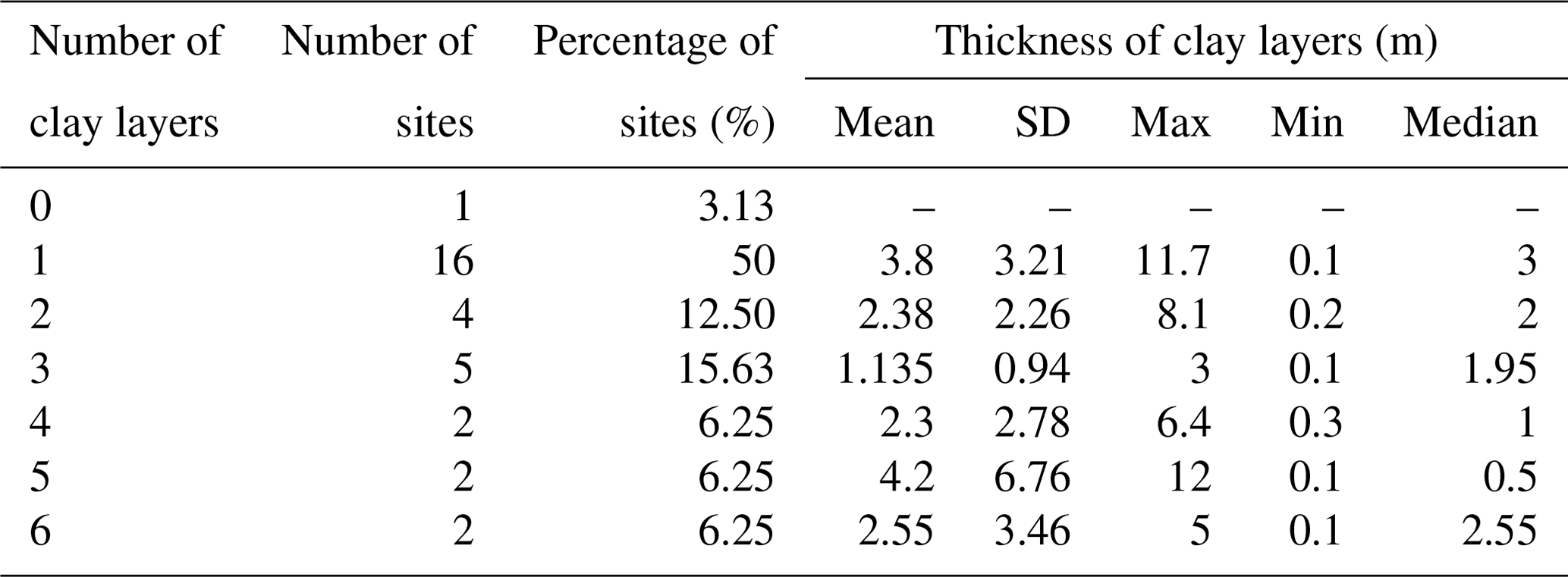
To create a representative configuration of the clay layers in the vadose zone above Israel's coastal plain aquifer, we examined the distribution of clay layers in selected fuel-contaminated sites. For that purpose, we constructed a database consisting of records obtained from the Israel Ministry of Environmental Protection from 32 fuel-contaminated sites containing dozens of monitoring boreholes. Each borehole in the database was sampled at multiple depths and characterized for the soil type. We classified these soil types into four main categories: gravel, sand, clayey sand (consisting of 55 % sand and 45 % clay), and clay, according to the soil type name on the database (see Table S9 in the Supplement for the categories). For each site, the percentage of each of the four soil types at each specific depth was extracted (i.e. the number of boreholes having a given soil type at a specific depth divided by the total number of boreholes penetrating that depth). We then recorded the percentage of clay at each depth; layers with a clay percentage higher than 25 % were considered clayey (Whiting et al., 2011). This yielded the number of clay layers and their thicknesses for each site (an example of one site is presented in Table S10 in the Supplement). Based on this methodology, the distribution of clay layers in contaminated sites at Israel's coastal plain vadose zone was calculated (Table 3).

Table 3 shows that only in 1 of the 32 examined sites had no clay layers at all. A proportion of 50 % of the sites only had one clay layer, and most of the sites had one to three layers (∼ 78 %), whereas almost 20 % had four to six layers. The mean of the layers' thickness ranged from 1–4 m. However, the standard deviation was high, and the actual thickness ranged from 11.7 to 0.1 m. Due to this variance in the distribution of clay layers (Table 3), it was decided to examine the number of clay layers (N) and their thickness (b) as additional input parameters in the sensitivity analysis of the heterogeneous media within the range of values reported in Table 3. The range of tested N and b can be found in Table 2. We are not aware of other studies that tested the distribution of clay layer interbeds in a SA for contaminant transport. However, Dai et al. (2017) tested the spatial distribution uncertainty of other parameters in a GSA, such as the elevations of the contact between aquifer and aquitard, the hourly head boundary conditions, and the hydraulic conductivity field.

The model was run for a total of either 100 years for the Morris analysis or 60 years for the Sobol analysis (in this case, the number of years was reduced to lower the overall high computational cost of the Sobol analysis). At the end of each run, the benzene concentration in the aquifer and the total flux to the aquifer were examined.

2.3 Global sensitivity analysis

2.3.1 The Morris method

The Morris or the elementary effect (EE) method was introduced by Morris (1991) and improved by Campolongo et al. (2007). It can be viewed as an extension of the OAT method, since it randomly generates sets of reference values from the entire parameter space and computes the difference of output (EE) caused by a fixed parameter change, altering only one parameter at a time. However, it can also be viewed as a GSA method, since it averages multiple EEs computed at different points in the parameter space. This method provides qualitative sensitivity measures (i.e. ranking the input parameters in order of importance); however it does not quantify the relative importance of each given parameter (Saltelli et al., 2004).

In the Morris method, each input parameter (x_i, where $i=\mathrm{1},\mathrm{\dots },k$), is assumed to vary across p selected levels in the space of the input parameter. The parameter space is normalized to a uniform distribution in [0,1] and partitioned into (p−1) equal sections. The algorithm starts at a randomly chosen point in the k-dimensional space and creates a trajectory (or a path) through the k-dimensional variable space. Each parameter is randomly chosen from the set (p−1) sections, and a fixed increment Δ (a multiple of $\mathrm{1}/(p-\mathrm{1})$) is added to each parameter in random order to compute an EE of each parameter, where EE is the difference of output y caused by the change Δ in the respective parameter. The EE for the ith input parameter can be described as

$$\begin{array}{}\text{(10)}& {\mathrm{EE}}_i\left(x_{\mathrm{1}}\mathrm{\dots }{x}_k\right)=\left({\displaystyle \frac{\begin{array}{c}Y(x_{\mathrm{1}},x_{\mathrm{2}},\mathrm{\dots },x_i+{\mathrm{\Delta }}_i,\mathrm{\dots },x_k)\\ -Y(x_{\mathrm{1}},x_{\mathrm{2}},\mathrm{\dots },x_i,\mathrm{\dots },x_k)\end{array}}{{\mathrm{\Delta }}_i}}\right).\end{array}$$

Changing each parameter once from one set of reference values completes one path, which together with the base case requires (k+1) simulations. Conducting simulations over multiple paths produces an ensemble of EE_is for each parameter. The number of required runs is then r(k+1), where r is the number of paths or trajectories. All EE_i values computed for randomly chosen paths are used to compute two final sensitivity measures ${\mathit{\mu }}_i^{\ast }$ and σ_i (Campolongo et al., 2007):

$$\begin{array}{}\text{(11)}& {\mathit{\mu }}_i^{\ast }={\displaystyle \frac{\mathrm{1}}{r}}\sum _{j=\mathrm{1}}^r\mathrm{|}{\mathrm{EE}}_{i,j}\mathrm{|},\end{array}$$

where ${\mathit{\mu }}_i^{\ast }$ is the mean of absolute values of the EE_i. ${\mathit{\mu }}_i^{\ast }$ can be regarded as a global sensitivity index, since it represents the average effect of each parameter over the parameter space. Thus, it is used to identify influential and non-influential parameters.

The second measure σ_i is the standard deviation of the EE_i:

$$\begin{array}{}\text{(12)}& {\mathit{\sigma }}_i=\sqrt{{\displaystyle \frac{\mathrm{1}}{r}}\sum _{j=\mathrm{1}}^r{\left({\mathrm{EE}}_{j,i}-{\displaystyle \frac{\mathrm{1}}{r}}\sum _{j=\mathrm{1}}^r\mathrm{|}{\mathrm{EE}}_{j,i}\mathrm{|}\right)}^{\mathrm{2}}}.\end{array}$$

It is used to identify non-linear and/or interaction effects.

The review by Song et al. (2015) reported that in different studies, the number of paths (r) varies from 20 to 1250 paths, representing a total of 280 to 40 000 numerical simulations, with an average of 500 paths. Both Brunetti et al. (2018) and Turco et al. (2017) combined the Hydrus model (1D and 2D, respectively) with the Morris method. Brunetti et al. (2018) set r=100 for a total of 1700 simulations, and Turco et al. (2017) set r=8 for a total of 40 simulations. In this study we set r=250, considering that the data will be further analysed by the Sobol GSA. This gave us a total number of 3000 and 4000 simulations for the analysis with and without clay layers, respectively.

2.3.2 The Sobol method

While the OAT and the Morris sensitivity methods are difference-based, the Sobol–Saltelli method is variance-based (Saltelli and Annoni, 2010). Variance-based methods are used to quantitatively identify both the importance of individual model parameters and parameter interactions. The Sobol method is based on a decomposition of the total model variance into two main elements: variance of the individual parameter and variance due to interaction with other parameters (Sobol, 2001). Decomposition of the model variance can be written as follows (Saltelli et al., 2004):

$$\begin{array}{}\text{(13)}& {\displaystyle }& {\displaystyle }V=\sum _{i=\mathrm{1}}^k{V}_i+\sum _{i=\mathrm{1}}^k\sum _{j>i}^k{V}_{ij}+\mathrm{\dots }{V}_{\mathrm{1},\mathrm{2},\mathrm{\dots },k}\text{(14)}& {\displaystyle }& {\displaystyle }{V}_i=V\left[E\right(Y\mathrm{|}{x}_i\left)\right]\text{(15)}& {\displaystyle }& {\displaystyle }{V}_{ij}=V\left[E\right(Y\mathrm{|}{x}_i{x}_j\left)\right]-V_i-V_j,\end{array}$$

where V stands for the total variance of the model output. V_i is the variance of each input parameter x_i, and E(Y|x_i) represents the mean of the system response Y when the parameter x_i is fixed at different values. V_ij represents the variance due to interactions between two parameters x_i and x_j, and V_1…k describes the variance among k parameters. These elements, represented by Sobol's sensitivity indices (SIs), provide quantitative information about the variance associated with a single parameter or related to interactions of multiple parameters. The main sensitivity index or the first-order sensitivity index S_i quantifies the main effect of parameter x_i on the total variance of Y, excluding the interactions with other parameters:

$$\begin{array}{}\text{(16)}& S_i={\displaystyle \frac{V_i}{V\left(Y\right)}}.\end{array}$$

The total-order sensitivity index $S_{T_i}$ of a single parameter x_i includes both the parameter's main variance effect and the proportion of the variance due to interactions of x_i with the other parameters:

$$\begin{array}{}\text{(17)}& S_{T_i}=S_i+\sum _{i\ne j}{S}_{ij}+\mathrm{\dots }+S_{\mathrm{1}\mathrm{\dots }k}.\end{array}$$

The values of the indices vary from 0 to 1, where 0 indicates no influence and 1 indicates a strong influence on the variance.

Parameter spaces were sampled using the Sobol quasi-random, cross-sampling strategy (Sobol, 2001). Rather than generating random numbers, this technique generates a uniform distribution in the probability space. The distribution appears qualitatively random, but sampling only takes place in regions of the probability function that were not previously sampled.

To assess the accuracy of the Sobol indices, confidence intervals of the indices should be constructed. The analytical procedure for confidence interval calculation involves repeating the r(2k+2) model runs several times, which was too time consuming and computationally demanding in this case. Therefore the bootstrapping approach was used instead (Efron and Tibshirani, 1986). Archer et al. (1997) suggested using bootstrap confidence intervals to produce confidence intervals of complicated data structures. The bootstrapping approach is based on resampling the parameter space of the data that are already available many times with replacement (randomly selecting values and allowing for duplicates) and constructing a distribution of the output (Efron and Tibshirani, 1986). Here, resamples were taken from the existing dataset Y with replacement, and the indices' values were recalculated. The result is an estimate of the mean and variance of each of the indices and allows us to calculate the confidence interval. The method thus relies on computational cost rather than on an analytical cost (running the model again). Here, the samples used for the model evaluation were resampled 1000 times with replacement, and 95 % confidence intervals were constructed (Archer et al., 1997).

Still, confidence intervals for the first-order indices (S₁) using the Sobol sampling method gave values of more than 100 %. This was also observed by Brunetti et al. (2016) and Hartmann et al. (2018), who also studied transport in unsaturated media. This may be a result of insufficient sample size, since Sobol's convergence requires a very large sample size (Saltelli et al., 2004). Therefore, we extracted S₁ values using the delta method developed by Plischke et al. (2013), by calculating S₁ values from given data through emulators and bootstrapping rather than running the model itself multiple times.

More details on the Sobol sample size can be found in the Supplement.

The Morris and the Sobol sensitivity analyses were executed using the Python programming language and, specifically, the Sensitivity Analysis Library (SALib) (Herman and Usher, 2017). SALib uses a Python script that overwrites the input parameters given by the GSA in the relevant Hydrus-1D model input files. The script then executes the model and returns the final aquifer solute concentration and the total solute flux to the aquifer at the end of the simulation. This procedure is repeated for the number of runs set for the GSA, with changes in the input parameters according to the sampling technique. SALib then computes the indices of the two methods: ${\mathit{\mu }}_i^{\ast }$ and σ_i and their confidence interval for the Morris method and the Sobol indices and their confidence interval for the Sobol method. Both Morris and Sobol methods have already been applied with the Hydrus software package by Périard et al. (2013; Hydrus-2D/3D), Brunetti et al. (2016, 2018; Hydrus-1D), Turco et al. (2017; Hydrus-2D), Hartmann et al. (2018; Hydrus-2D), and others.

2.4 Treatment of missing output data

Owing to the arbitrary choice of input parameters and multiple model runs, the model sometimes does not converge and crashes. This makes data analysis problematic because sampling order is important for the analysis results of most GSA methods. Since there is not yet an agreed and established way of handling these missing data (Sheikholeslami et al., 2019), we tested the following methods:

Missing data removal. This method consists of removing the missing data points, or by removing full trajectories, so that the order of sampling within trajectories remains undisturbed. However, by removing data, valuable information can be lost. In addition, in most methods, removing data may render the entire sample since it no longer follows the sampling sequence and data structure. Thus, this study only tested value removal for the Morris method where full trajectories can be removed.

Missing data imputation. A missing value is replaced with some other value. The following missing data imputation approaches were tested.

1. Constant value substitution is an easy and computationally cheap method for imputing missing data. The missing data can be replaced with zeros in cases where the output is typically near zero or with the mean or the median, in cases where the distribution is skewed. Sheikholeslami et al. (2019) for example, used the median substitution technique for a rainfall-runoff model and a land surface hydrology model. A shortcoming of this replacement methods is the potential for reducing the variance and distorting other statistical properties of the output (Sheikholeslami et al., 2019). In this study, both the zero and the median substitutions gave similar final GSA indices, with slightly different confidence intervals. Therefore, only the zero substitution results are presented.

2. The K nearest-neighbour (KNN) substitution technique uses neighbourhood observations to fill in missing data. The underlying rationale behind the KNN-based techniques is that the sample points closer to x_i should provide better information for imputing the failed output, where x_i is an input parameter vector for which a simulation model fails to return an outcome. In the KNN method, the failed output is replaced by a response value of a weighted average of the K (the number of samples) nearest neighbours. The KNN algorithm computes the distance of the test observation to every observation in the K nearest neighbours and then imputes the missing value with the average model response of K simulations (Duneja and Puyalnithi, 2017). The computed neighbouring distance between the samples is typically the Euclidean distance (Duneja and Puyalnithi, 2017; Troyanskaya et al., 2001). Lower K values generally result in predictions with high variance and low bias and vice versa for high K values (Hastie et al., 2009). Thus, in this study, we tested both a lower K value of 5, as was used by Shapiro and Day-Lewis (2022) for groundwater hydrology models, and a higher K equal to the square root of the size of the dataset – a rule of thumb in the KNN method reported to correctly distinguish signal from noise (Duneja and Puyalnithi, 2017). The KNN analysis was conducted using the programming language Python with the scikit-learn KNN regressor.

3. RBF emulation-based substitution – model emulation or surrogate modelling – is a strategy that develops statistical, cheap-to-run surrogates for the output of complex, computationally intensive models (Razavi et al., 2012a). The emulator usually uses a low computational cost function that fits the non-missing response values Y_a to predict the values for the missing response Y_m. There are various types of model emulations that can be used for hydrological models such as polynomial regressions, kriging, artificial neural networks, RBFs, and support vector machines (Razavi et al., 2012; Zhou et al., 2022). The RBF is one of the most commonly used function approximation techniques because it can provide an accurate emulation of high-dimensional problems for a low computational cost. Sheikholeslami et al. (2019), for example, employed the RBF approximation for crashed model simulation emulation, which performed better than all other methods tested in that study. The RBF approximation is a weighted summation of n_a number of functions that can approximate the predictive response Y at a point x_i. Here n_a was set to the number of non-missing sample points. Detailed equations of the RBF approximation can be found in the Supplement. The RBF imputation analysis was also conducted with the Python program using the SciPy RBF interpolation package.

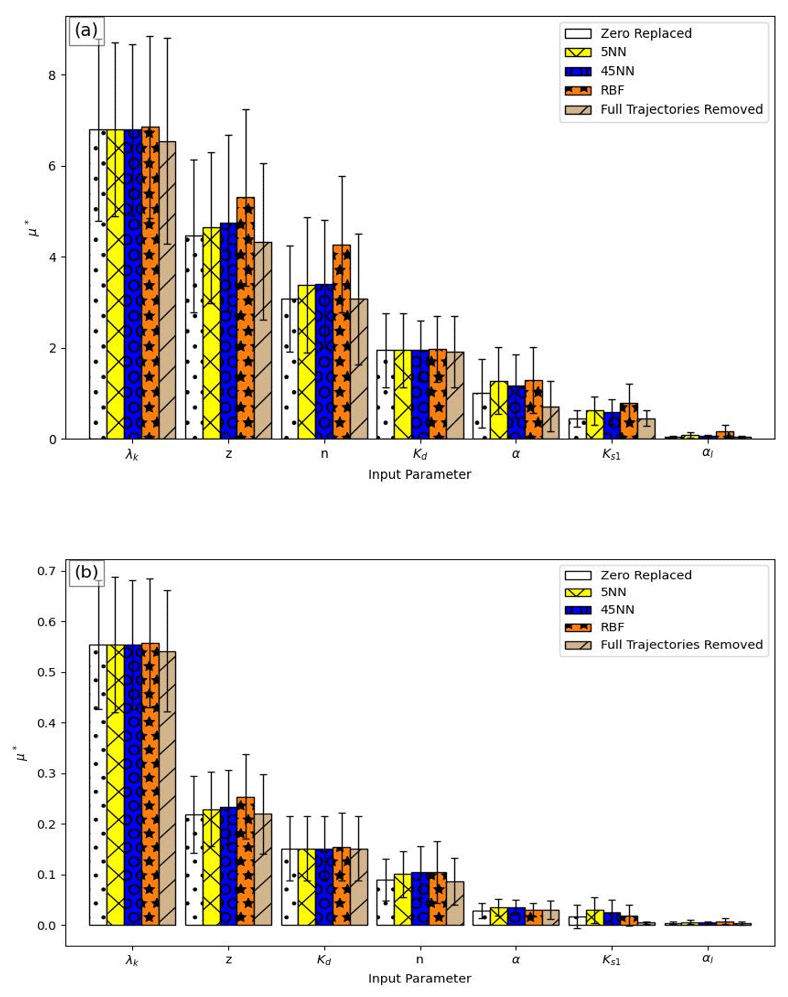
Figure 2 Morris analysis results for homogenous sandy soil obtained using different methods for missing data imputation/removal for (a) cumulative benzene flux to the aquifer and (b) final benzene concentration in the aquifer. Black bars represent μ^∗ confidence intervals.

3 Results and discussion

3.1 Homogenous media analyses

3.1.1 Morris analysis for homogenous sandy soil

In this analysis, the model's sensitivity to seven input parameters (k) was tested (Table 2), considering two model outputs: benzene aquifer concentration at the end of the simulation and benzene cumulative flux to the aquifer. The analysis was conducted for 250 paths (r) and six levels (p; i.e. dividing the parameters' space to five equal segments, where the parameter can be assigned six different values) for 2000 simulations overall (r(k+1)). Out of these simulations, only 42 simulations (2.1 %) did not converge or crashed. To avoid bias in the results, we used the methodology described in Sect. 2.4 to either replace the missing values or remove the trajectories that contain missing values. Three imputation methods are presented: zero substitution, the RBF emulator, and the KNN method with K=5 and K=45 (representing the square root of the sample size). Figure 2 presents μ^∗ for these different methods. Detailed values of all indices for the different methods can be found in the Supplement (Tables S3 and S4). Small differences were observed between the different methods for the values of μ^∗, the μ^∗ confidence interval, and σ, for each of the input parameters, with the same order of parameter importance. The similarity between the different methods stems from the scarce missing values, hardly affecting the overall results. In all strategies for handling missing data, it is evident that the GSA performed worst for the weakly influential parameters – α, K_s, and α_l, exhibiting a high ratio of the μ^∗ confidence interval to μ^∗ (Fig. 2, Tables S3 and S4). This was also evident in global sensitivity analyses obtained using the Hydrus model for other hydrological problems (Brunetti et al., 2016, 2022; Hartmann et al., 2018; Zhou et al., 2022; Brunetti et al., 2017).

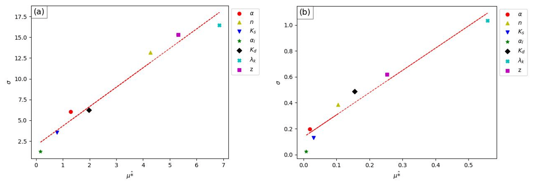
Figure 3 Morris analysis results for homogenous sandy soil with RBF imputation for (a) cumulative benzene flux to the aquifer and (b) final benzene concentration in the aquifer.

The effect of the different parameters on the output can also be seen in Fig. 3a and b, where μ^∗ versus σ is presented for the Morris analysis conducted with the RBF emulation substitution method used to replace the crashed data. Though minimal differences were observed among all methods (Fig. 2), the RBF results are shown here for consistency purposes, since the RBF method gave the best results in the heterogeneous media case (see Sect. 3.2).

In all cases, the input parameter with the strongest effect on the system was the degradation rate λ_k, followed by the profile depth z (Figs. 2 and 3). The next two influential parameters are the adsorption coefficient K_d and the van Genuchten n parameter. Both showed a similar effect on the concentration, though the effect of n on the flux to the aquifer was much more pronounced and K_d was slightly more influential for the concentration. Finally, the van Genuchten α parameter, the hydraulic conductivity K_s, and the dispersivity α_l showed little effect on the model results.

Zanello et al. (2021) reported similar results in a LSA for a model of BTEX transport in an unsaturated homogenous sandy soil using Hydrus-2D/3D software. They found that the order of the input parameters' influence on BTEX arrival to the aquifer (tested as concentration) was ${\mathit{\lambda }}_k>K_{\mathrm{d}}>z>K_{\mathrm{s}}$. The stronger influence of K_d compared to z in that study is probably due to the low z values tested there (2.5–4 m), representing a shallow aquifer. In another study, Davis et al. (1994) modelled the constant leakage of benzene in a loamy sand soil to an aquifer beneath a manufacturing facility. Benzene concentrations of ∼ 1 mg L⁻¹ were found in the groundwater beneath the source (∼ 25 mg L⁻¹), though in monitoring wells ∼ 100 m from the source no benzene was detected. In their LSA, they too found that λ_k was the dominant mechanism for benzene attenuation and found K_d to be very influential. Moreover, similarly to our study, their model was insensitive to α_l (Davis et al., 1994). Indeed, the great importance of biodegradation for the removal of petrol hydrocarbons in aerobic environments has been recognized and reported in the literature (Lahvis et al., 1999; Berlin et al., 2016; Yadav and Hassanizadeh, 2011; Berlin and Suresh, 2019; Alvarez et al., 1991; Abu Hamed et al., 2004). This result is demonstrated once again in our study.

Generally, the order of influence of the parameters was similar for the cumulative flux to the aquifer and for the final concentration in the aquifer (Fig. 3), except for K_d and n as stated above. For both the flux and the concentration, a correlation between μ^∗ and σ is observed, as reflected in their arrangement around the same diagonal line (Fig. 3, red line), indicating that none of the parameters have solely a linear effect (μ^∗ being the mean effect). Instead, all parameters exhibit an interaction effect (σ – the standard deviation of the effect), where the interactions increases with the increase in the mean.

3.1.2 Sobol analysis for homogenous sandy soil

The Sobol analysis for homogenous media was conducted for the four most influential parameters of the Morris analysis: λ_k, z, n, and K_d, to obtain more quantitative information on the parameters' influence and interactions. A total of 5000 sets of parameters were generated, constituting an overall total of 50 000 model runs for r(2k+2). Of the 50 000 model runs, 881 samples did not converge. The same methodology used for the Morris analysis was used for imputation of missing values (Sect. 2.4). However, with the Sobol analysis, it was impossible to remove the missing points, since the order of sampling is significant to the overall analysis, and sampling is not divided into sets of trajectories. Hence, the data removal method was not used.

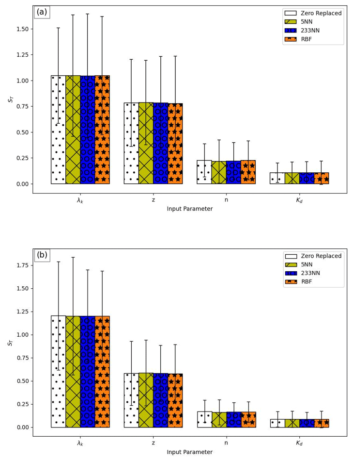
Figure 4 The Sobol total indices (S_T) for homogenous sandy soil obtained using different methods for missing data imputation for (a) cumulative benzene flux to the aquifer and (b) final benzene concentration in the aquifer. Black bars represent S_T confidence intervals.

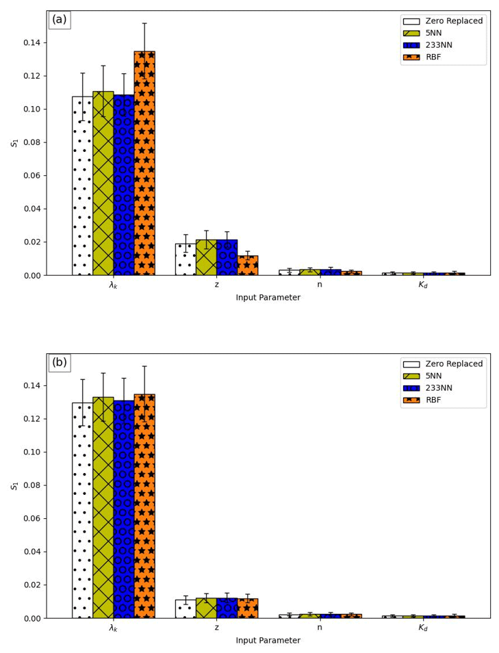
Figure 5 Sobol first-order indices (S₁) for homogenous sandy soil obtained using different methods for missing data imputation for (a) cumulative benzene flux to the aquifer and (b) final benzene concentration in the aquifer. Black bars represent μ^∗ confidence intervals.

Figures 4 and 5 show the S₁ and S_T Sobol indices for the different methods of missing data replacement. Detailed and averaged values of all methods can be found in the Supplement (Tables S5–S8). All missing data imputation methods gave similar results (Figs. 4 and 5 and Tables S5–S8). This is expected given the low dimensionality of the model (four input parameters). Here, the GSA also performed the worst for the weakly influential parameters (n and K_d) exhibiting a high ratio of the confidence interval to indices.

A similar effect of the different parameters' order and magnitude of importance on the two outputs was observed. Like the Morris analysis, λ_k and z were found to be the most influential parameters with the highest total-order (S_T) and first-order (S₁) index values (Figs. 4 and 5). S_T, unlike S₁, often sums to more than 100 % because it is the sum of S₁ and all the higher-order Sobol indices involving the parameter (Saltelli et al., 2004). The difference S_T−S₁ is a measure of how much parameter x_i is involved in interactions with any other input variable (Saltelli et al., 2004). The total index S_T (Figs. 4 and 5) demonstrates that most of the variance in both flux and concentration is caused by λ_k, consisting of the variation of λ_k itself (S₁ of ∼ 11.38 % and 13.21 % for the flux and concentration, respectively; Tables S5 and S6) and the interactions with other parameters. It should be noted that z has a relatively low main effect (S₁ of 1.85 % and 1.17 % for the flux and concentration, respectively; Tables S5 and S6) but a high total effect of ∼ 58 % and 78 % for the flux and concentration, respectively (Tables S7 and S8), indicating that this parameter has a limited direct impact on the variance of the output but a strong interaction effect, most likely with the degradation coefficient. The total Sobol index of an input parameter is the sum of the first-order Sobol index and all the higher-order Sobol' indices involving that parameter. Hence, the sum of the total Sobol sensitivity indices is equal to or greater than 1 (Gatel et al., 2020). If no higher-order interactions are present, the sum of both the first- and total-order Sobol indices is equal to 1. Sums of S_T values > 100 % were also reported by Brunetti et al. (2017), Schübl et al. (2022), Zhou et al. (2022), and Nossent et al. (2011).

Ciriello et al. (2017) performed a Sobol analysis for benzene contamination in an unsaturated soil assuming a very deep aquifer that contamination does not reach and in a shallow aquifer. They reported K_s as one of the most important parameters, while α and n were both found to be mostly insignificant. However, it is hard to compare that study and this one because λ_k, K_d, and z which were found to be highly significant in this study were not tested in that study. In addition, we tested moderate aquifer depths (more than 5 m).

λ_k is the only parameter with S₁ higher than 10 % and hence the only parameter with a strong main effect on the output variance. When the sum of all first-order indices is less than 100 %, the model is non-additive, meaning that it is affected by interactions (Neumann, 2012; Nossent et al., 2011). Here, the sum of all first-order indices is < 15 %, indicating that the model is non-additive and very much affected by interactions. Only 13.7 % and 14.8 % of the variance for the flux and concentration, respectively, are attributable to the first-order effect (Tables S5 and S6; showing the sum of S₁ for the flux and concentration, respectively), highlighting the fundamental role of interactions between parameters.

Overall, the Sobol method results agreed with those of the Morris method. Indeed, the Morris method was proposed as an efficient tool to be used prior to variance-based GSA, in order to screen important and unimportant factors and to provide the first inspection of the model's behaviour at a reasonable computational cost (Brunetti et al., 2018; Song et al., 2015; Wainwright et al., 2013). Similarities between Morris and variance-based methods were also observed by Herman et al. (2013) and Sarrazin et al. (2016).

3.2 Heterogeneous media

Morris analysis for heterogeneous media

In this analysis, 12 parameters concerning the soil type were examined, α, n, K_s, α_l, λ_k, and K_d, both for sand and clayey soil (represented below with a subscript of 1 and 2, respectively). Three additional general profile parameters were tested, z, N, and b, comprising 15 parameters overall (Table 2).

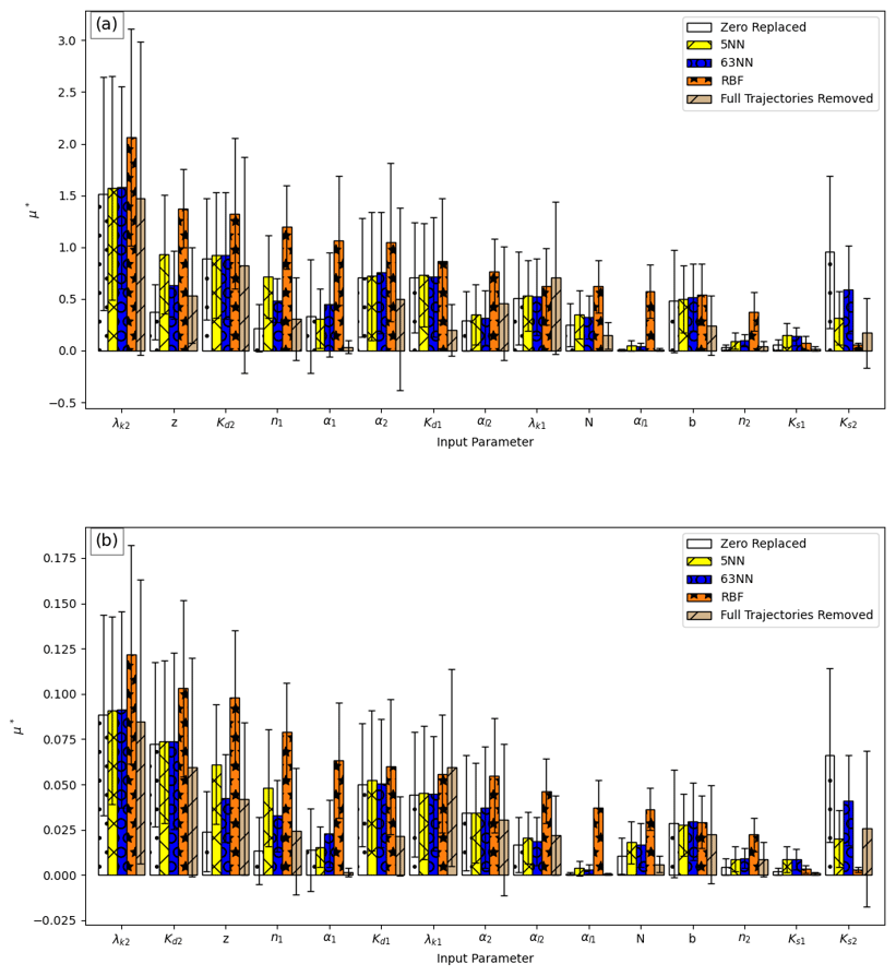
Figure 6 Morris analysis results for heterogeneous media: μ^∗ values for (a) cumulative benzene flux to the aquifer and (b) final benzene concentration in the aquifer.

The analysis was conducted for 250 paths (r) and four levels for an overall total of 4000 simulations (r(k+1)), from which 959 did not converge or crashed. The increase in the ratio of failures compared with the previous analysis (2.1 % for the homogeneous Morris analysis versus ∼ 24 % here) can be attributed to the complex transport in the heterogeneous medium and the difficulty in modelling flow between sand and clay layers, as well as to the increase in the number of model parameters (dimensionality of the parameter space) increasing the arbitrary combinations of parameters during GSA (Sheikholeslami et al., 2019). The same methodology was used for missing data imputation or removal, as discussed above. Unlike the previous analyses, the different methods for missing values imputation yielded dissimilar confidence interval levels, as well as dissimilar μ^∗ values for some parameters (Fig. 6). Also, an overall increase in the ratio between μ^∗ and its confidence interval was observed (Fig. 6). In the Supplement, the ratio between the μ^∗ confidence interval and μ^∗ is presented in Fig. S2 in the Supplement to clearly illustrate the difference between the different methods and parameters. GSA results with high confidence interval values were also reported by other studies that used Hydrus models (Brunetti et al., 2016, 2022; Hartmann et al., 2018; Zhou et al., 2022; Brunetti et al., 2017). Though the authors do not address this issue, it indicates that more model runs are needed for the indices to converge (Sarrazin et al., 2016). Yet, a clear μ^∗ ranking is observed, with an overall consistency with the previous results of the homogeneous case and among the different methods.

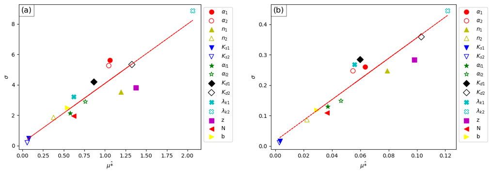
Figure 7 Morris analysis results for heterogeneous media for (a) cumulative benzene flux to the aquifer and (b) final benzene concentration in the aquifer.

Full trajectory removal performed the poorest for most parameters, while the RBF emulation method performed the best (Figs. 6 and S2). The two KNN methods gave better results than the zero substitution. These results are similar to those reported by Sheikholeslami et al. (2019), in which the RBF-emulation-based substitution performed better than the single NN and than a constant value substitution (the median, in their case). Detailed values of all methods' indices can be found in the Supplement (Tables S11 and S12). A correlation between μ^∗ and σ for all input parameters is again demonstrated by their arrangement around one diagonal line (the red line in Fig. 7a and b), indicating that the interactions' effect increases with the increase in the total effect of each parameter.

Figure 7a and b show the effect of the different parameters on the outputs, in terms of μ^∗ versus σ, using the RBF method. Like the GSA results of the homogenous media, it is evident that the degradation coefficient λ_k2, the sorption coefficient K_d2 of the clay soil, the depth z, and the van Genuchten n₁ parameter of the sand layers are the most dominant factors controlling benzene transport to the aquifer. The degradation coefficient of the clay layers λ_k2 was found to be the most dominant parameter, considering both the cumulative flux and the concentration at the end of the simulation. The sorption coefficient of the clay layers K_d2 is second-most influential for the concentration but equally important as the depth z, which comes in third place for the flux, followed by n₁ in fourth place. Benzene adsorption for clay minerals is higher than that for sand (Berlin and Suresh, 2019; Zytner, 1994) and was set accordingly in the GSA (Table 1); therefore, its overall increased influence is not surprising, as well as the increased influence of λ_k2 in these layers, as the solute is attenuated due to sorption. The stronger effect of K_d2 on the concentration as compared with the flux is expected, since sorption directly affects the solute concentration. On the other hand, n₁ of the sand was much more influential than n₂, probably since it is a parameter affecting the flow, and sand comprises most of the profile. We note that these four parameters were also found to be significant for homogenous soil analysis; thus, they should be carefully examined when modelling the fate and transport of benzene.

A large group of moderately influential parameters follow these four most influential parameters. For the flux, α₁ and α₂ follow in importance in fifth and sixth place, followed by the sand adsorption coefficient K_d1, which comes in seventh place. For the concentration, α₂ is also at the fifth place; however, K_d1 and λ_k1 are more influential and come in sixth and seventh place, respectively, also showing a greater degree of interaction effect, just before α₁ at the eighth place. The parameters K_d1 and λ_k1 are likely to affect concentration more than flux, since they affect benzene directly, similarly to K_d2 here and K_d1 in the homogenous media analysis. They both lower benzene concentrations but have less effect on the total flux.

Following these influential parameters, the dispersivities α_l2 and α_l1 of both soil types are less influential but still somewhat close to the middle of the graph, together with clay layers distribution parameters, b and N, and with λ_k1 for the flux. The least influential parameters are n₂ of the clay layer and the hydraulic conductivities of both soil types, K_s1 and K_s2. Interestingly, Gribb et al. (2002), who conducted LSA for a risk assessment model of benzene and naphthalene transport to groundwater through sand, loam, and clay soils, also reported high model sensitivity to λ_k and K_d for all soils. In their case, the model was also less sensitive to K_s, except for pure loam and clay soils. For other parameters that were not tested here (porosity, bulk density, residual water content, and initial concentration), the model was only sensitive in the case of pure clayey soil. However, their study assumed homogenous media of each soil type, which may have obscured the effect of a specific parameter for different soil types in a single profile. In the present study, it is also evident that λ_k and K_d are very influential, depending also on the soil type, whereas K_s is the least influential parameter.

The results for both the homogenous and heterogeneous media indicate that the most dominant factor controlling benzene arrival to the aquifer is λ_k, the rate of benzene removal from the media by biological degradation. This rate can vary greatly from extremely fast to very slow rates, depending on parameters such as initial benzene concentration and soil water content (Table S1). In general, the degradation rate is lower for higher concentrations and lower water content, and vice versa. Since the values of λ_k vary greatly in the literature, this parameter must be carefully selected in hydrological modelling for benzene transport, and further research to elucidate its value onsite is encouraged.

The parameters z, K_d, and n₁ followed λ_k in importance; K_d usually had a stronger effect on the concentration than on the flux. The aquifer depth is an easy-to-measure parameter, and it should be included in any model for benzene transport. Likewise, n can be evaluated quite easily using tools such as Rosetta to establish soil texture (Schaap et al., 2001). The adsorption coefficient of the clay layers was also found to be highly significant. Therefore, examination and characterization of the onsite soil types are also extremely important. Most studies that tested SA for benzene transport in different soils types used homogenous media representation of each soil type and tested one soil type at a time (Davis et al., 1994; Gatel et al., 2019; Gribb et al., 2002). In this study, we tested the effects of both parameters of the individual soil types and the distribution of the clay layers using b and N. Thus, we offer an improved assessment of the importance of each parameter of each soil type and show that clay layer should be represented and characterized, though the exact layering distribution is only moderately influential. On the other hand, literature values may be used for non-influential parameters, including the hydraulic conductivities K_s1 and K_s2 and n₂.

4 Summary and conclusions

This paper explores the effect of different model parameters on benzene transport in the vadose zone of Israel's coastal plain aquifer and its potential arrival to the aquifer below. A physical model was implemented to simulate benzene transport in the unsaturated zone. The model was initially employed for homogenous sandy soil, as sand comprises the vast majority of the vadose zone. Next, the model was set to describe heterogeneous soil containing clay layers representing lithology obtained from data of contaminated sites. Two GSA methods were applied to examine the effect of the model input parameters on benzene concentration in the aquifer at the end of the simulation and on benzene cumulative flux to the aquifer. Additionally, treatment of missing data due to model crashes was demonstrated.

The results for both the homogenous and heterogeneous media showed that the most dominant factor controlling benzene arrival to the aquifer is benzene degradation coefficient (λ_k). Following λ_k, the depth (z) of the aquifer was highly significant. The adsorption coefficient K_d and van Genuchten n parameter of the sand soil were also found to be highly significant.

A substantial interaction effect between the parameters was observed; the parameters with the highest individual effect showed a high interaction effect and vice versa. The degree of individual parameter influence on the model was shown to be small (< 15 %) by the Sobol analysis, indicating the great importance of interactions between parameters.

The different methods for missing data handling yielded a similar overall ranking of the influential parameters identified by the GSA. However, the RBF-emulation-based substitution showed better results compared to the KNN and zero substitution techniques, particularly when the transport between layers was considered, and the model dimensionality and subsequent number of failures were high. In that case, the data removal technique performed markedly worse.