the Creative Commons Attribution 4.0 License.
the Creative Commons Attribution 4.0 License.
 | 09 Jan 2024
Projecting sediment export from two highly glacierized alpine catchments under climate change: exploring non-parametric regression as an analysis tool
Lena Katharina Schmidt
Till Francke
Peter Martin Grosse
Axel Bronstert
Future changes in suspended sediment export from deglaciating high-alpine catchments affect downstream hydropower reservoirs, flood hazard, ecosystems and water quality. Yet, quantitative projections of future sediment export have so far been hindered by the lack of process-based models that can take into account all relevant processes within the complex systems determining sediment dynamics at the catchment scale. As a promising alternative, machine-learning (ML) approaches have recently been successfully applied to modeling suspended sediment yields (SSYs).
This study is the first, to our knowledge, exploring a machine-learning approach to derive sediment export projections until the year 2100. We employ quantile regression forest (QRF), which proved to be a powerful method to model past SSYs in previous studies, for two nested glaciated high-alpine catchments in the Ötztal, Austria, above gauge Vent (98.1 km2) and gauge Vernagt (11.4 km2). As predictors, we use temperature and precipitation projections (EURO-CORDEX) and discharge projections (AMUNDSEN physically based hydroclimatological and snow model) for the two gauges. We address uncertainties associated with the known limitation of QRF that underestimates can be expected if values in the projection period exceed the range represented in the training data (out-of-observation-range days, OOOR). For this, we assess the frequency and extent of these exceedances and the sensitivity of the resulting mean annual suspended sediment concentration (SSC) estimates. We examine the resulting SSY projections for trends, the estimated timing of peak sediment and changes in the seasonal distribution.
Our results show that the uncertainties associated with the OOOR data points are small before 2070 (max. 3 % change in estimated mean annual SSC). Results after 2070 have to be treated more cautiously as OOOR data points occur more frequently, and glaciers are projected to have (nearly) vanished by then in some projections, which likely substantially alters sediment dynamics in the area. The resulting projections suggest decreasing sediment export at both gauges in the coming decades, regardless of the emission scenario, which implies that peak sediment has already passed or is underway. This is linked to substantial decreases in discharge volumes, especially during the glacier melt phase in late summer, as a result of increasing temperatures and thus shrinking glaciers. Nevertheless, high(er) annual yields can occur in response to heavy summer precipitation, and both developments would need to be considered in managing sediments, as well as e.g., flood hazard. While we chose the predictors to act as proxies for sediment-relevant processes, future studies are encouraged to try and include geomorphological changes more explicitly, e.g., changes in connectivity, landsliding, rockfalls or vegetation colonization, as these could improve the reliability of the projections.
- Article
(5005 KB) - Full-text XML
- BibTeX
- EndNote


Fluvial suspended sediment export from glacierized, high-alpine areas can be up to 1 order of magnitude higher (per unit area) than in non-glacierized downstream areas (Hinderer et al., 2013; Beniston et al., 2018). Thus, sediment dynamics in these high-alpine areas and changes therein have important implications for downstream hydropower generation and reservoir sedimentation (Schöber and Hofer, 2018; Guillén-Ludeña et al., 2018; Li et al., 2022), water quality (as well as nutrient and contaminant transport) (Bilotta and Brazier, 2008), aquatic species and riverine ecosystems (Milner et al., 2009, 2017; Gabbud and Lane, 2016; Huss et al., 2017), and also flood hazard (Nones, 2019) and carbon cycling (Tan et al., 2017; Syvitski et al., 2022).
High-alpine areas are particularly sensitive to climate change, experiencing above-average warming (Gobiet et al., 2014) and hence crucial cryospheric changes, such as ongoing and accelerating deglaciation, permafrost melt, and snow cover changes (Huss et al., 2017; Beniston et al., 2018; Abermann et al., 2009). These changes induce changes in discharge volumes, timing and magnitude (Vormoor et al., 2015; Kuhn et al., 2016; van Tiel et al., 2019; Rottler et al., 2020; Hanus et al., 2021). This in turn affects sediment export, and past changes have been observed frequently, e.g., due to enhanced subglacial sediment evacuation and increased sediment availability in expanding erodible landscapes as receding glaciers and melting permafrost e.g., expose glacial till and weaken rockwalls (Micheletti and Lane, 2016; Carrivick and Heckmann, 2017; Lane et al., 2017, 2019; Costa et al., 2018; Delaney and Adhikari, 2020; Li et al., 2020; Vergara et al., 2022).
Nevertheless, future changes in sediment export are understudied (Zhang et al., 2022), and questions such as “Are sediment yields from deglaciating catchments increasing, decreasing or is there no pattern?” or “to what extent is it possible to quantify spatio-temporal patterns of future sediment yields?” (Carrivick and Tweed, 2021) have yet to be answered – although projections of climatological (e.g., Gobiet and Kotlarski, 2020; Gobiet et al., 2014), glaciological (e.g., Stoll et al., 2020; Bolibar et al., 2022; Huss, 2011) and hydrological changes (e.g., Madsen et al., 2014; Hanzer et al., 2018; Hanus et al., 2021; Huss and Hock, 2018; Tecklenburg et al., 2012; Wijngaard et al., 2016), which could serve as a basis for estimating future changes in sediment export, are numerous.
The main reason why answering such questions is challenging is that modeling sediment export at the catchment scale with process-based models remains difficult – if not impossible – because it is determined by a complex system of interconnected processes that is not straightforward to model. For example, the relationship between suspended sediment concentrations and discharge is most often nonlinear in time and space, and univariate models relying solely on discharge are often insufficient (Vercruysse et al., 2017; Zhang et al., 2021). Hence, in addition to variations in discharge, changes in sediment availability, entrainment, transport and deposition would have to be considered; there may be threshold effects and nonlinear responses of geomorphic processes (e.g., triggering of mass movements), correlated influencing factors, hysteresis and seasonality (Huggel et al., 2012; Landers and Sturm, 2013; Vercruysse et al., 2017; Costa et al., 2018; Schmidt et al., 2023; Zhang et al., 2022). Additionally, long-term field observations (i.e., several decades and covering a wide range of conditions) that provide enough training and validation data to develop sediment yield models or to analyze trends are very rare (Zhang et al., 2022; Schmidt et al., 2023).
There are conceptual models on (suspended) sediment export from deglaciating areas (Antoniazza and Lane, 2021; Carrivick and Tweed, 2021; Zhang et al., 2022), which expect an initial increase in sediment export as glaciers begin to retreat and an eventual decrease – after peak sediment – once the glaciers have disappeared and the landscape stabilizes. The timing of peak sediment relative to peak meltwater and the completion of deglaciation is presumed to depend on changes in erosive precipitation; i.e., a negative trend in erosive precipitation implies that peak meltwater and peak sediment may co-occur, while a positive trend or no change in erosive precipitation result in a lag between peak meltwater and peak sediment. However, deducing estimates of future sediment export and implications for individual catchments based on these conceptual considerations is not straightforward or even possible.
Common approaches to model sediment yields at the catchment scale, such as SWAT (e.g., Vigiak et al., 2017), BQART (Syvitski and Milliman, 2007), WBMsed (Cohen et al., 2013), WASA-SED (Mueller et al., 2010) or SAT (Zhang et al., 2021), are mostly empirical or conceptual in their sediment modules, do not consider all relevant erosion processes (i.e., neglecting glacial, gully erosion and landslides in the case of SWAT), and often concentrate on large spatial scales (i.e., sediment fluxes to the oceans for large basins, entire continents or at global scale) and/or large temporal scales (i.e., multiyear averages and long-term fluxes). On the other end of the spectrum, models for individual parts or processes within glacierized catchments exist as, for example, a numerical approach to model subglacial fluvial sediment transport (Delaney et al., 2019) that has also been coupled with models for ice dynamics and bedrock erosion (Delaney et al., 2021) or, e.g., probabilistic or physical models of mass wasting processes, such as landslide or debris flows (Iverson and George, 2014; Hirschberg et al., 2021; Campforts et al., 2022). However, as of yet, there is no all-in-one physical model (fully distributed, incorporating thermal and pluvial drivers of sediment mobilization and transport) to simulate sediment export from cryospheric basins (Zhang et al., 2022) at the catchment scale.
Accordingly, studies that have attempted to project future suspended sediment yields (SSYs) chose rather qualitative approaches, such as comparing sediment yield observations of warmer and colder ablation seasons (Stott and Mount, 2007; Bogen, 2008) and using the responses of SSYs to past predictor changes and applying these to projected changes in the future (Li et al., 2021b) or fitting a multiple regression model to past data (of only 1 year) and increasing the temperature input in the model (Stott and Convey, 2021). However, these approaches may preclude modeling decreases or accounting for interactions between variables.
As a promising alternative, geoscientific machine-learning approaches have emerged and have recently been acknowledged for their potential in applications to Earth system science (Reichstein et al., 2019). Indeed, first studies showed that machine-learning approaches can easily outperform well-known existing models for sediment yield (Gupta et al., 2021; Rahman et al., 2022; Jimeno-Sáez et al., 2022; Schmidt et al., 2023). Such black-box approaches tend to perform well for black-box problems such as high-alpine sediment dynamics, “where the input data and output data are well understood or at least fairly simple, yet the process that relates the input to output is extremely complex” (Lantz, 2019). In a previous study, we have developed and validated a quantile regression forest (QRF) approach to model SSYs in two nested high-alpine catchments and to estimate yields for the past 5 decades (Schmidt et al., 2023). This showed that the QRF model outperformed commonly applied sediment rating curves by about 20 % of explained variance, and other studies found that regression trees and random forest models (which QRF is based on) even outperformed other machine learning approaches in modeling sediment dynamics (Talebi et al., 2017; Al-Mukhtar, 2019).
Thus, the present study is motivated to explore QRF to model future SSYs based on measurement data, emission scenarios and subsequent hydrological model results. We test the approach in two glacierized high-alpine catchments in the Ötztal in Austria, where projections of future climatological and glacio-hydrological conditions from the AMUNDSEN model are available (Hanzer et al., 2018) and where we have successfully trained and applied QRF models to reconstruct past sediment export using records of discharge, precipitation and air temperature (Schmidt et al., 2023).
The goals of the present study are (i) to assess uncertainties of the model due to known limitations of the QRF method in order to identify the limitations of the approach and (ii) to derive estimates of future changes in sediment export with respect to trends in annual yields, shifts in the seasonal distribution and the timing of peak sediment.
In a previous study, we trained and validated quantile regression forest models to retrospectively estimate SSYs at two gauges for the past 5 decades using the available records of turbidity-derived suspended sediment concentrations (4 and 15 years) and long-term records of the predictors, i.e., discharge, precipitation and temperature (Schmidt et al., 2023) (Fig. 2, dashed-line box). In the present study, we use these models and apply them to downscaled and bias-corrected EURO-CORDEX temperature and precipitation projections that were used as input data for the glacio-hydrological model AMUNDSEN, as well as the discharge projections of AMUNDSEN (Hanzer et al., 2018) (Fig. 1). In the following, we outline the quantile regression forest approach including its advantages and limitations with respect to modeling suspended sediment dynamics and the choice of predictors to model sediment dynamics in high-alpine areas. Then, we describe the study area, input data and necessary adjustments, as well as how we analyzed the limitations, sensitivities and the resulting SSY estimates.
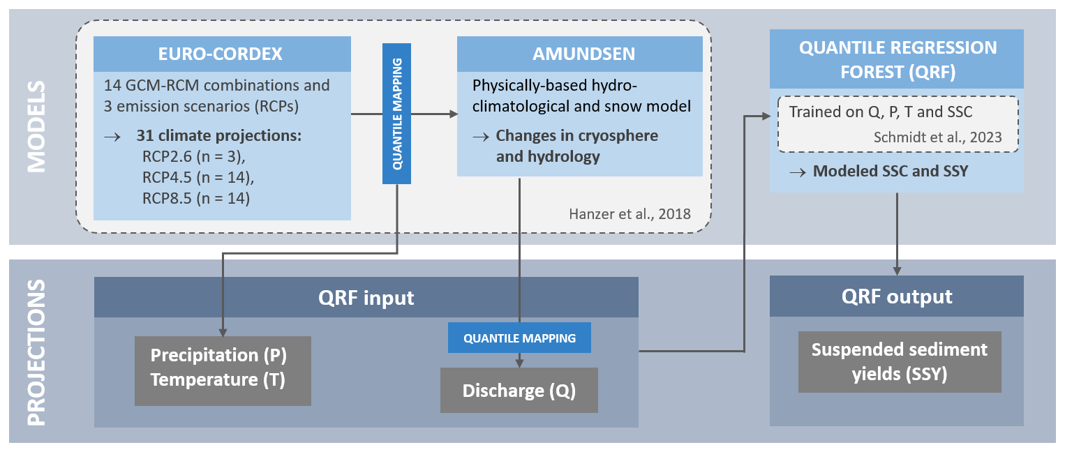
Figure 1Overview of models and resulting projections used in this study. Bias-corrected EURO-CORDEX climate projections and AMUNDSEN model results serve as input data for the QRF models. Q: discharge, P: precipitation, T: temperature, SSC: suspended sediment concentrations, SSY: suspended sediment yields.
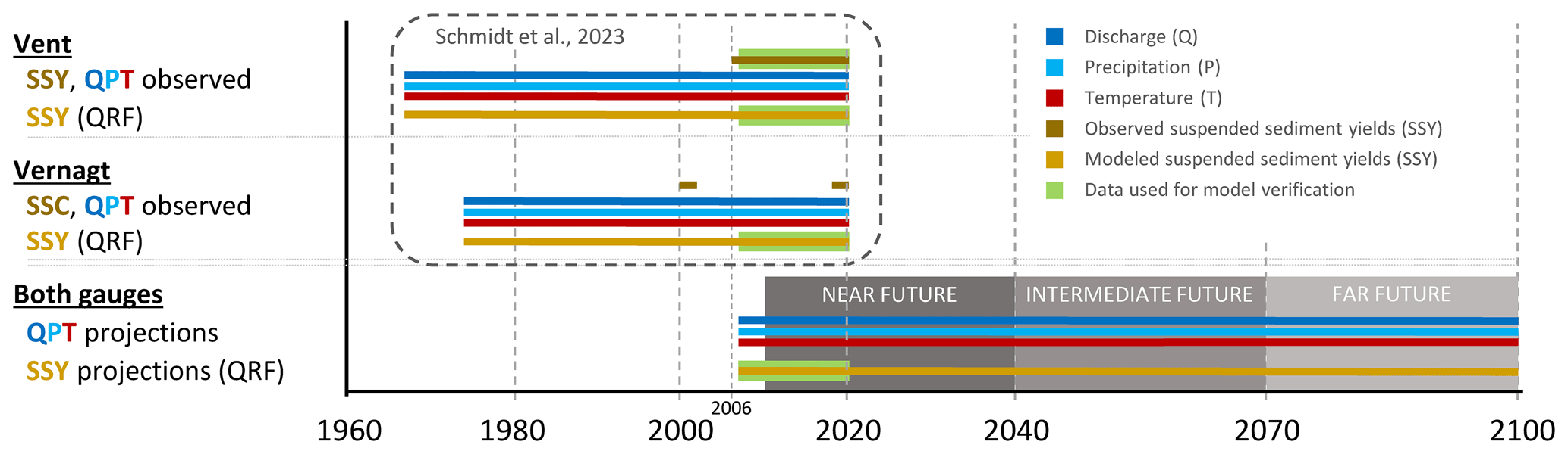
Figure 2Temporal extent of input data, as well as modeled suspended sediment yields (SSYs) in the previous study (dashed-line box, top left) and projections (discharge Q, precipitation P, temperature T) as input data and SSY estimates from this study; 2006–2020 is the training data period at gauge Vent. At gauge Vernagt, the QRF model was trained on the years 2000, 2001, 2019 and 2020, when SSC data were available. Thus, to verify model results in the present study, we use the QRF estimated yields at gauge Vernagt of the years overlapping with the climate and hydrology projections, i.e., the overlap period of 2007–2020 (Sect. 2.4.1).
2.1 Quantile regression forest for suspended sediment concentration modeling
The quantile regression forest (QRF) (Meinshausen, 2006) is a non-parametric regression technique that is based on random forests (RFs) and can be classified as a machine-learning approach. It learns from the training data by growing ensembles of regression trees on random subsets (bootstrap samples) of the training data (Francke et al., 2008a; Schmidt et al., 2023). In each regression tree, the data are recursively partitioned based on splitting rules, where both RF and QRF randomly select the predictors used for splitting. In contrast to random forests, QRF keeps all observations within a node (whereas RF only keeps the mean), which allows us to construct prediction intervals and to assess uncertainty (Schmidt et al., 2023).
The advantages of QRF include that it can handle multiple input variables; makes no assumptions on distributions; and can deal with interactions, nonlinearity and non-additive behavior. In terms of limitations, it does not allow for easy interpretation of the effects of single predictors, and model predictions will always be within the range of observations, i.e., if the predictors in the period of application exceed the range represented in the training data set (hereafter called out-of-observation-range (OOOR) data points), we can expect overestimations or underestimations of the target variable if the respective predictor has a continuing monotonic effect in this range (Schmidt et al., 2023).
With respect to modeling suspended sediment concentrations, studies have shown that QRF is very well suited to modeling sedigraphs and estimating annual SSY (Francke et al., 2008b, a; Zimmermann et al., 2012) and that it performs favorably compared to sediment rating curves and generalized linear models (Francke et al., 2008a; Schmidt et al., 2023). On a related note, RF (which QRF is based on) outperformed support vector machines and artificial neural networks (Al-Mukhtar, 2019) in modeling suspended sediment concentrations.
In a previous study (Schmidt et al., 2023), we trained QRF models at daily resolution on data of the two gauges Vent and Vernagt using the limited available time series of turbidity (4 and 15 years) and long records of the primary predictors, namely discharge (Q), precipitation (P) and air temperature (T) (Fig. 2). These can be seen as drivers or proxies for processes and catchment conditions crucial to sediment dynamics in high-alpine areas: e.g., discharge determines sediment transfer and erosion within the channel; precipitation is key for runoff formation and hillslope erosion, hillslope–channel coupling and the triggering of mass movement events; and air temperature controls the activation of sediment sources (e.g., sub- and proglacial sediments and their transport by glacier meltwaters or hillslope destabilization by permafrost thaw) and whether precipitation occurs as rain or snow. In addition to these primary predictors, we derived ancillary predictors to describe antecedent conditions and the cumulative effects thereof: e.g., longer-term discharge behavior may exhaust sediment sources or lead to sediment storage, long warm periods may deplete snow cover and accelerate glacier melt associated with increased subglacial sediment transport, and high antecedent moisture conditions may amplify surface runoff or promote mass movements in response to precipitation events. To capture these antecedent conditions while keeping the correlation between the derived predictors as low as possible, we computed sums of the primary predictors in non-overlapping windows of increasing sizes (e.g., 24, 24–72, 72 h to 7 d and 7 to 20 d ahead of each time step) (Schmidt et al., 2023; Zimmermann et al., 2012). The lengths of the considered time periods differ between the models as we optimized them for the highest model performance using the Nash–Sutcliffe efficiency (Schmidt et al., 2023). Additionally, we used the day of the year to capture the seasonality and the rate of change in discharge as predictors (Francke et al., 2008b). The models were validated at both gauges. At gauge Vernagt, we trained validation models on the two available 2-year training data sets (2000–2001 and 2019–2020) and compared the model estimates to measurements from the respective period not included in the training data (NSE of 0.73 and 0.6 for daily SSY; for details, see Schmidt et al., 2023). At gauge Vent, a 5-fold cross-validation demonstrated the superior performance compared to sediment rating curves, especially in periods containing threshold effects due to extreme events. For the past 5 decades, OOOR data points (see Sect. 2.4.2) were rare, which strengthened the notion that the available training data covered the majority of typical situations.
2.2 Study area
The two studied gauges Vent Rofenache (hereafter Vent, operated by the Hydrographic Service of Tyrol) and Vernagt (operated by the Bavarian Academy of Sciences and Humanities) are located in the Rofental in the Ötztal Alps, Austria (Fig. 3). The two corresponding nested catchments of 98.1 and 11.4 km2 span elevations ranging from 1891 m a.s.l. at gauge Vent and 2635 m a.s.l. at gauge Vernagt to 3772 m a.s.l. The area is characterized by a relatively warm and dry climate (for this alpine setting), with a mean annual temperature of 2.5 ∘C at gauge Vent (Strasser et al., 2018) and average annual precipitation as low as 660 mm at gauge Vent but a strong precipitation gradient with elevation (Schmidt et al., 2023). Both catchments are heavily glacierized (28 % and 64 % glacier cover in 2015 (Buckel and Otto, 2018)), but accelerating glacier retreat has been observed since the beginning of the 1980s (Escher-Vetter, 2007; Braun et al., 2007; Abermann et al., 2009). Apart from the glaciers, land cover at high elevations is dominated by bare rock or sparsely vegetated terrain, whereas mountain pastures and coniferous forests occupy lower elevations. Geology is dominated by biotite-plagioclase, biotite and muscovite gneisses, variable mica schists, and gneissic schists (Strasser et al., 2018).
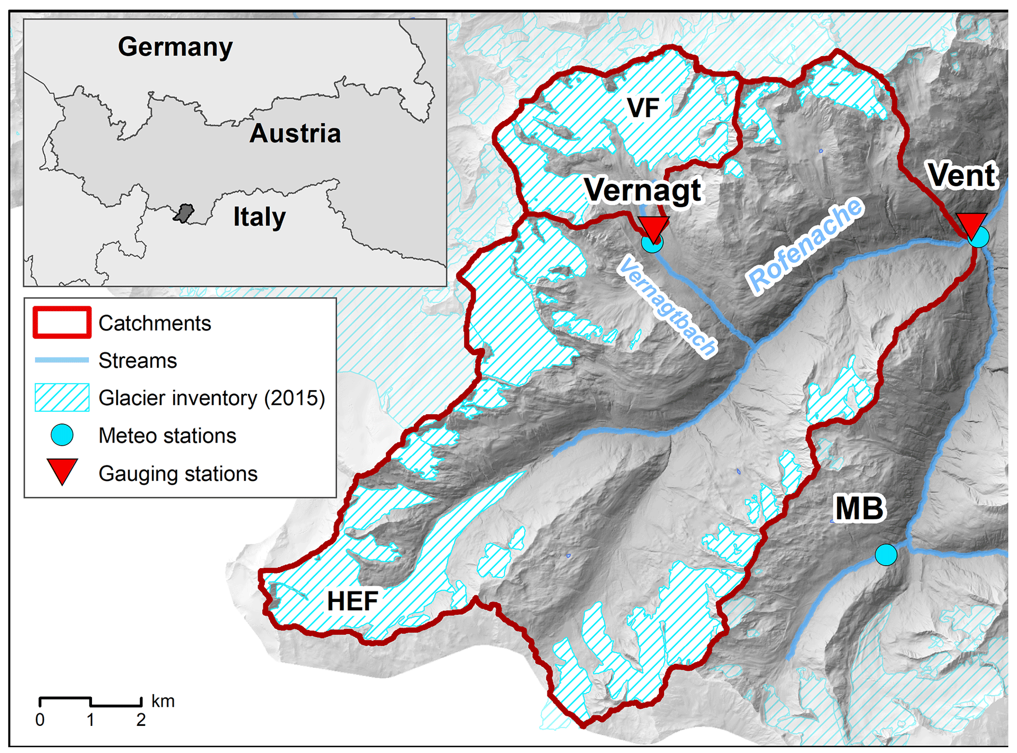
Figure 3Map of the catchment area above gauge Vent, with nested catchment above gauge Vernagt and major glaciers Vernagtferner (VF) and Hintereisferner (HEF). Meteo stations recording precipitation and temperature are located close to the gauges. Map based on 10 m DEM of Tirol (Land Tirol, 2016), glacier inventory of 2015 (Buckel and Otto, 2018) and river network from tiris open government data (Land Tirol, 2021).
The river Rofenache is a tributary stream of the Ötztaler Ache, one of the largest tributaries to the river Inn. The glacial-to-nival hydrological regime shows a pronounced seasonality, with almost 90 % of discharge occurring during snow and glacier melt from April to September (Schmidt et al., 2023). Mean annual suspended sediment concentrations at gauge Vent were the highest in an Austria-wide comparison (Lalk et al., 2014). Annual suspended sediment yields in Vent averaged 1500 t km−2 a−1 with an even more pronounced seasonality compared to discharge (99 % of the annual SSY transported from April to September) (Schmidt et al., 2023).
2.3 Input data
2.3.1 Climate projections
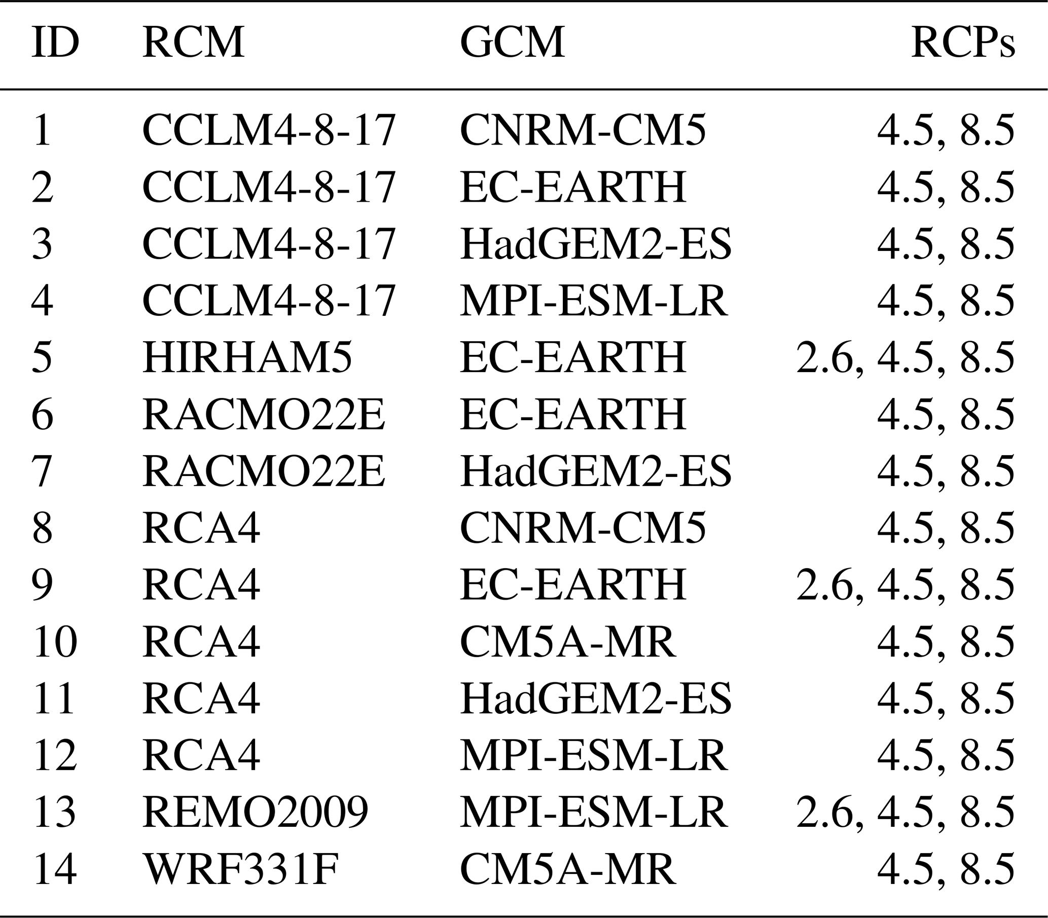
We used projections of air temperature and precipitation of the European part of the COordinated Regional Downscaling Experiment (EURO-CORDEX) (Jacob et al., 2014), which have been downscaled and bias-corrected for use in their hydrological model by Hanzer et al. (2018). The EURO-CORDEX initiative provides regional climate model results to enable exploration of the impacts of future climate change at a comparatively high horizontal resolution. This is beneficial for modeling future sediment export, for example since regional climate model simulations provide higher precipitation intensities, which are entirely missing in the global climate model simulations (Jacob et al., 2014), and are thus more likely to capture erosion-relevant changes in precipitation. The data used in this study and by Hanzer et al. (2018) were the result of six different regional climate models (RCMs) driven by five different global climate models (GCMs), resulting in a total of 14 different GCM–RCM modeling chains (Table 1). These are forced by three different emission scenarios expressed as representative concentration pathways (RCPs), which correspond to added radiative forcings of 2.6, 4.5 and 8.5 W m−2 at the end of the 21st century relative to pre-industrial conditions, i.e., RCP2.6 (intervention scenario assuming peak CO2 concentrations in the middle of the century, followed by slow decline and negative emissions), RCP4.5 (intermediate scenario with peak emissions mid-century followed by strong decline) and RCP8.5 (assuming no implementation of climate mitigation policies, considerably and steadily increasing emissions and greenhouse gas concentrations over time) (Jacob et al., 2014; Hanzer et al., 2018). This results in a total of 31 RCP–GCM–RCM combinations. The horizontal resolution of the original EURO-CORDEX projections is 0.11∘ (≈ 12.5 km).
Table 1Overview of EURO-CORDEX scenario simulations used in this study (unaltered from Hanzer et al., 2018, and distributed under CC BY 3.0, https://creativecommons.org/licenses/by/3.0/, last access: 22 December 2023).
Hanzer et al. (2018) used statistical downscaling to represent the local scale. For this, they bias-corrected all RCM outputs using at least 20 years of observations in the period 1971 to 2005 by using quantile mapping, which matches the distributions of the climate model simulations of the current climate to the distributions of observations. This is necessary, especially in Alpine regions, because the 12.5 km spatial resolution of RCMs (despite being comparatively high) cannot sufficiently resolve topographical and climatological heterogeneities (Hirschberg et al., 2021). Hanzer et al. (2018) concluded that the corrected RCM outputs adequately represent the mean and variability of the observed climate. They interpolated the meteorology to a 100 m grid, and we used the projections for the two grid cells that are located closest to the gauges Vent and Vernagt. EURO-CORDEX simulations are provided at daily resolution, and Hanzer et al. (2018), have disaggregated them to 3 h resolution to capture diurnal variability in the energy fluxes. We re-aggregated these data to a daily resolution to match the temporal resolution of our QRF models (see Sect. 2.3.3).
2.3.2 Hydrological projections
We used discharge projections of the physically based hydroclimatological and snow model AMUNDSEN (Hanzer et al., 2018), which is a fully distributed energy and mass balance model including glacier evolution (Δ h method) and that is particularly adapted to high-mountain catchments on a small to regional scale. It comprises a glacier retreat module and has been extensively validated for historic conditions, especially with respect to snow distribution (Hanzer et al., 2016). This is especially beneficial for modeling sediment dynamics since AMUNDSEN can model processes such as changes in glacier melt that govern discharge dynamics and are crucial to sediment fluxes in these high-alpine areas. AMUNDSEN was forced by the downscaled, bias-corrected and temporally disaggregated EURO-CORDEX simulations of precipitation and air temperature described above (as well as relative humidity, global radiation and wind speed) and modeled snow, glaciers and hydrology in the Ötztal Alps until 2100 (Hanzer et al., 2016). The AMUNDSEN model was calibrated and extensively validated for the period 1997–2013 using water-balance-derived mean areal precipitation, snow depth recordings, Landsat- and MODIS-derived snow extent maps, glacier mass balances, and runoff recordings (Hanzer et al., 2016).
The temporal extent of both the meteorological and the hydrological projections is 2006 to 2100, but since data are not available for the entire year of 2006, we use the period of 2007 to 2100. Additionally, three HadGEM-driven models ended in November 2099. The years 2007 to 2020 overlap with observation data at gauge Vent and the results of the previous study at gauge Vernagt (Fig. 2), which we utilize to verify our model results (see Sects. 2.4.1 and 3.2).
2.3.3 Adjustment of input data for the QRF model
As the QRF models were trained at daily resolution, we aggregated the Q and T projections from 3 h resolution to daily means and the P projections to daily sums. However, comparing the AMUNDSEN Q projections to observations in the overlap period (2007–2020; see Fig. 2) showed underestimation of Q during the glacier melt period at gauge Vernagt and substantial overestimation of Q during the snowmelt period at gauge Vent. Hanzer et al. (2018) have acknowledged that but have left the overestimations (percent bias, PBIAS, of up to 23 %) unaltered since “mainly changes rather than absolute values are analyzed; these partial model biases likely do not affect the main conclusions”. However, in our case, it is necessary to correct the discharge data since SSYs are sensitive to discharge amounts, and additionally, unrealistic discharge amounts exceeding the maximum discharge value in the training data represent a challenge (see Sect. 2.4.2). Also, it is necessary to represent discharge seasonality and thus discharge origins as accurately as possible as, usually, more sediment is exported during glacier melt than at similar discharge levels during snowmelt (Schmidt et al., 2023).
For consistency, we applied the same bias correction as Hanzer et al. (2018), i.e., quantile mapping, using the methodology by Gudmundsson et al. (2012) as implemented in the R package qmap (Gudmundsson, 2016). Due to strong season-dependent biases, Hanzer et al. (2018) have performed quantile mapping for each season individually. We followed this approach, yet in order to best represent discharge seasonality, we shifted the limits of the seasons by 1 month (NDJ, FMA, MJJ and ASO instead of DJF, MAM, JJA and SON) as this corresponded better to seasons with similar characteristics of overestimation or underestimation.
2.4 Analyses of model limitations and uncertainties
To analyze model performance and identify the limits of the applicability of the presented QRF modeling approach, we verified the modeled SSYs against measurement data in the overlap period (2007–2020) (Sect. 2.4.1); assessed the frequency of OOOR data points, including by how much the observation range of the predictors is exceeded in the projections; and analyzed whether the modeled SSY are sensitive to changes in these predictors (Sect. 2.4.2).
2.4.1 Verification of model results based on observed data
To determine how well the obtained SSY projections correspond to SSY derived from turbidity measurements, we compared the model results in the overlap period (2007 to 2020) to measurements at gauge Vent. Lacking continuous direct measurements at gauge Vernagt, we used estimated SSYs for the years 2007–2020 from the QRF model trained on measurements for the years 2000, 2001, 2019 and 2020 (Schmidt et al., 2023) for the comparison (see also Fig. 2). To simplify the descriptions in the results, we hereafter refer to these estimates as observations as well. As the hydroclimatic projections (and, thus, the SSY projections resulting thereof) do not mimic the characteristics of single years (let alone months or days) but merely reproduce their distribution, we compared the distributions of observed and simulated annual SSYs. To test for significant differences between these distributions, we used the two-sample Kolmogorov–Smirnov test, which is able to handle the non-normal distribution of some groups, as implemented in the R package stats version 3.5.1 (R Core Team, 2018). Additionally, we assessed whether the seasonality of sediment export is accurately represented in the model results by comparing mean monthly SSY.
2.4.2 Assessment of limits of applicability
As mentioned in Sect. 2.1, a known limitation of QRF is that model bias can result if the predictors in the projection period exceed the range of observed values used as training data. This limitation is a direct consequence of the numerical characteristics of RF and QRF, which are incapable of extrapolation. In order to assess how often and to what extent the model results are affected, we performed a series of analyses (overview in Fig. 4), described in the following.

Figure 4Overview of analyses performed with respect to OOOR days. Max(xp,train) denotes the maximum value in the training data, n refers to the number of OOOR days, and e refers to the exceedance extent. Subscripts are as follows: p for predictor, rcp for emission scenario, and ts for time slice. The analysis of OOOR precipitation days (3) is described in Sect. 2.5.
Analysis of out-of-observation-range days
First, we quantified how often OOOR days occurred for each projection proj and predictor p (i.e., Q, P or T) as the mean annual number of OOOR days per year:
where nyears is the number of years, and is the number of OOOR days in a given predictor and projection in a given year i. Additionally, we determined the exceedance extent (percentage of the maximum value in the training data max(xp,train)), i.e., by how much the maxima in the observations (i.e., the training period) max(xp,train) were exceeded on the OOOR days j (i.e., in the projection period):
where xp,j is the value of the predictor p on OOOR day j.
Although the same limitations of QRF theoretically also apply to predictors falling below the training minima, we did not consider them since Q and P already contained very low or zero values and cannot fall below zero. Likewise, for T, minimum temperatures are already well below zero, and a further decrease (if it occurs) is not further physically relevant to sediment transport. Similarly, we only considered summer precipitation at both gauges (i.e., May–September) to exclude snowfall events that are not directly relevant to sediment dynamics.
Sensitivity analysis
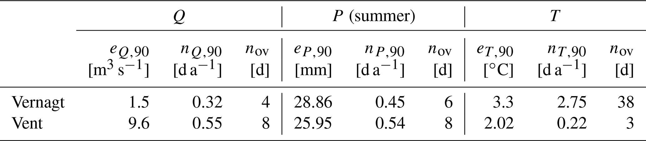
To assess the potential effects of the abovementioned OOOR days on the model results, we performed a sensitivity analysis for the three primary predictors Q, P and T (Fig. 4). For this, we determined the 90th percentiles of the number of OOOR days and the exceedance extents ep,j of all projections, i.e., np,90 (in d a−1) and ep,90 (in % of max(xp,train)), for each predictor p. These values were considered to represent a severe case for possible model deficits due to their lacking extrapolation capability. We created a respective test data set for the sensitivity analysis from the training data in the 14-year overlap period (2007–2020): we selected the corresponding number of days nov with the highest values of the respective predictor in the overlap period, as
and altered them by adding or subtracting the respective ep,90. For example, np,90 of Q in Vent is 0.55 d a−1; therefore, we changed nov= 0.55 ⋅ 14 ≈ 8 d by the ep,90 of 9.6 m3 s−1 (Table 2).
Table 2Amount of reduction or increase in the sensitivity models (average exceedance extent in units of the corresponding predictor) and number of days with a reduction or increase on average per year () and in total in the 14-year period (nov).
We used the resulting altered time series of the primary predictors to compute the corresponding ancillary predictors (that describe antecedent conditions; see Sect. 2.1), ran the QRF model with them and compared mean annual SSC after the alterations to the original data set. Thus, we performed six individual runs for the sensitivity assessment at each gauge, two (one where the predictor was increased and one where it was reduced) for each of the three primary predictors Q, P and T. We chose to compare mean annual SSC instead of annual SSY as discharge is needed to compute SSY so that the alterations in Q would have affected the estimated SSY twice.
Classification
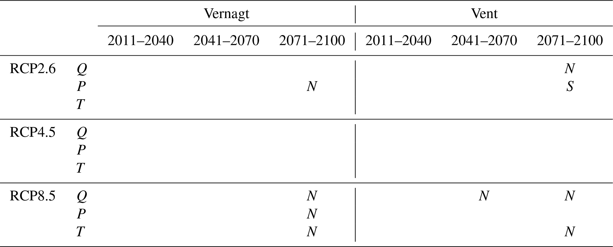
Third, we assessed whether the sensitivity analysis was informative for the different RCPs, time slices and predictors, i.e., if the sensitivity analyses contained sufficiently extreme conditions to represent the projections. For this, we determined the mean exceedance extent per predictor p, emission scenario rcp and time slice ts and the mean number of OOOR days per year . We compared these to the ep,90 and np,90 and marked the respective predictor–time-slice–RCP combination with N or S in Table 5 if ≥ of projections or and with bold N or S if this applied to ≥ of the projections (see Fig. 5 and Table 5).
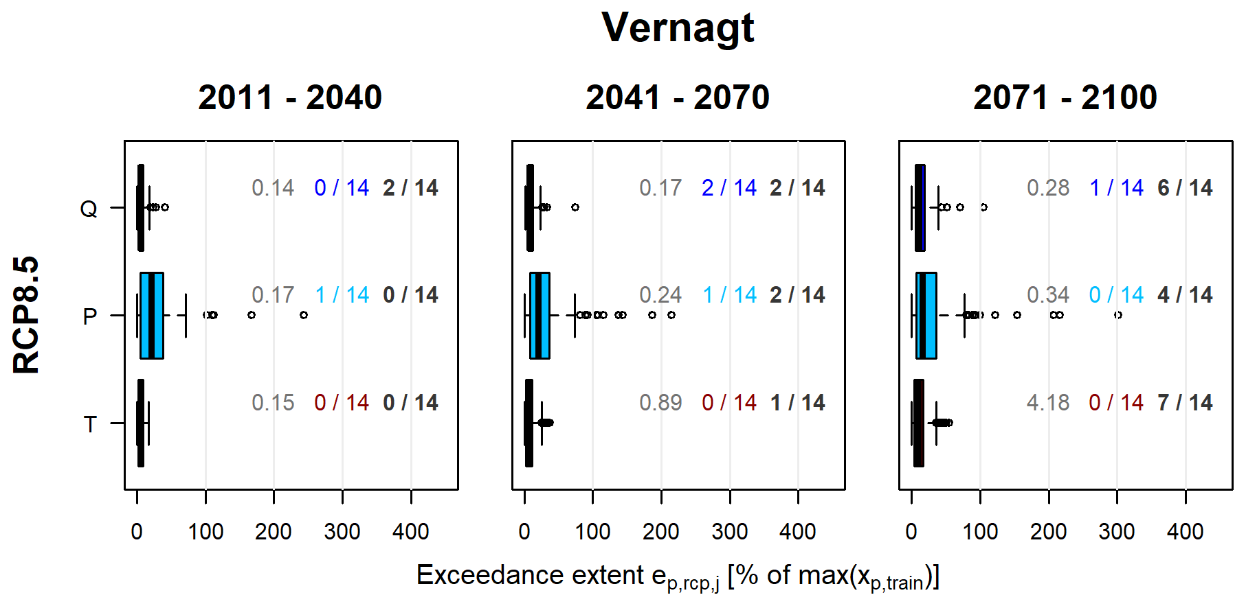
Figure 5Example of the classification based on the OOOR analysis. The boxplots show the distribution of exceedance extents per RCP and predictor on all days j within the respective time slice ts. Gray numbers denote the average of all projections within the respective RCP, time slice and predictor. Colored numbers indicate the number of projections with the mean exceedance extent , i.e., projections more extreme than the sensitivity analysis. Black numbers indicate the number or projections with the mean number of OOOR days per year , i.e., projections with more OOOR days than the sensitivity analysis.
2.5 Analysis of model results
We analyzed the model results, i.e., estimated annual yields in the projection period for trends, as well as shifts in seasonality. To assess trends, we used two methods implemented in the R package FUME (Santander Meteorology Group, 2012): the Mann–Kendall test, which is a non-parametric tool to detect linear trends (specifically, we used a version that was modified to detect trends in serially correlated time series; Madsen et al., 2014; Yue et al., 2012) and Sen's slope estimator (Sen, 1968) to assess trend magnitude. Further, we compared the estimated yields in three time slices (near future: 2011–2040, intermediate future: 2041–2070, and far future: 2071–2100; see also Fig. 2), comparable e.g., to Jacob et al. (2014) and Hanzer et al. (2018). To assess changes or shifts in the seasonality of sediment export, we compared the mean monthly yields of the observations and the projections.
To assess whether the detected trends are sensitive to the potential underestimation of yields on OOOR precipitation days, we multiplied the daily yields estimated by our QRF model on these days by a factor of 5, i.e., assuming a very severe underestimation in the original estimates (Fig. 4). We chose this factor as it is close to the most severe exceedance extents in precipitation at both gauges, which are 456 % at gauge Vernagt and 442 % at gauge Vent (see also Sect. 3.3). We then compared the trends in annual SSY of the altered time series to the trends in the original QRF estimates. All analyses were conducted with the statistical software R (R Core Team, 2018).
3.1 Verification of bias-corrected discharge for the present climate (2007–2020)
The bias-corrected discharge data yield more adequate representations of measured monthly discharge amounts and their seasonal distribution (Fig. 6), as well as mean annual discharge volumes (Table 3). At gauge Vernagt, for example, maximum mean monthly Q in the observations and the bias-corrected data is in August, whereas the original AMUNDSEN simulations suggested a maximum in July. Nevertheless, some underestimation of August discharge remains at gauge Vernagt. At gauge Vent, the original AMUNDSEN simulations substantially overestimated discharge amounts in April to July, i.e., the snowmelt period, which was successfully corrected by the bias correction.
Table 3Comparison of mean annual discharge volumes based on the original AMUNDSEN output, observations and bias-corrected AMUNDSEN estimates in the overlap period (2007–2020).
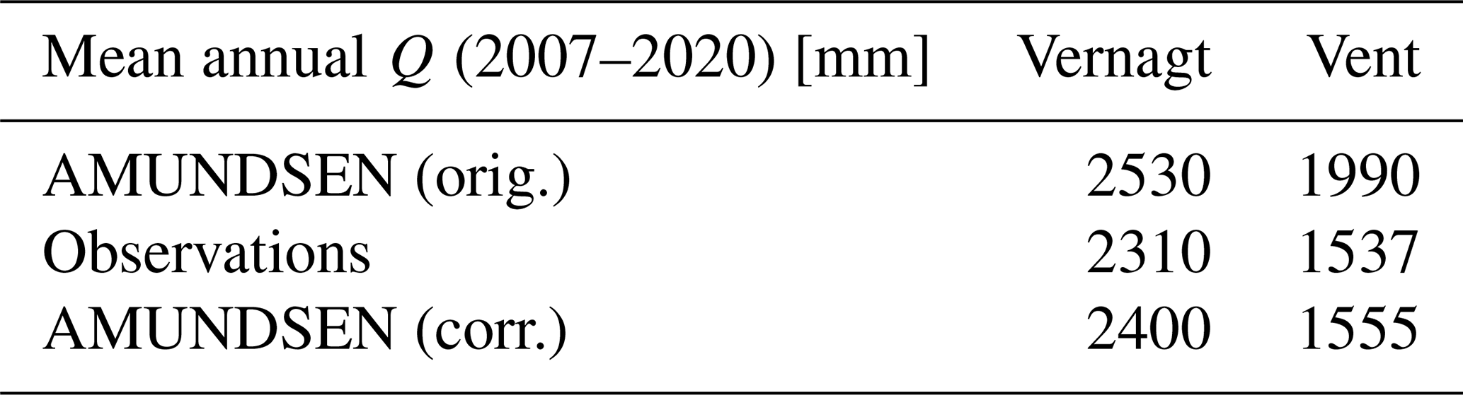
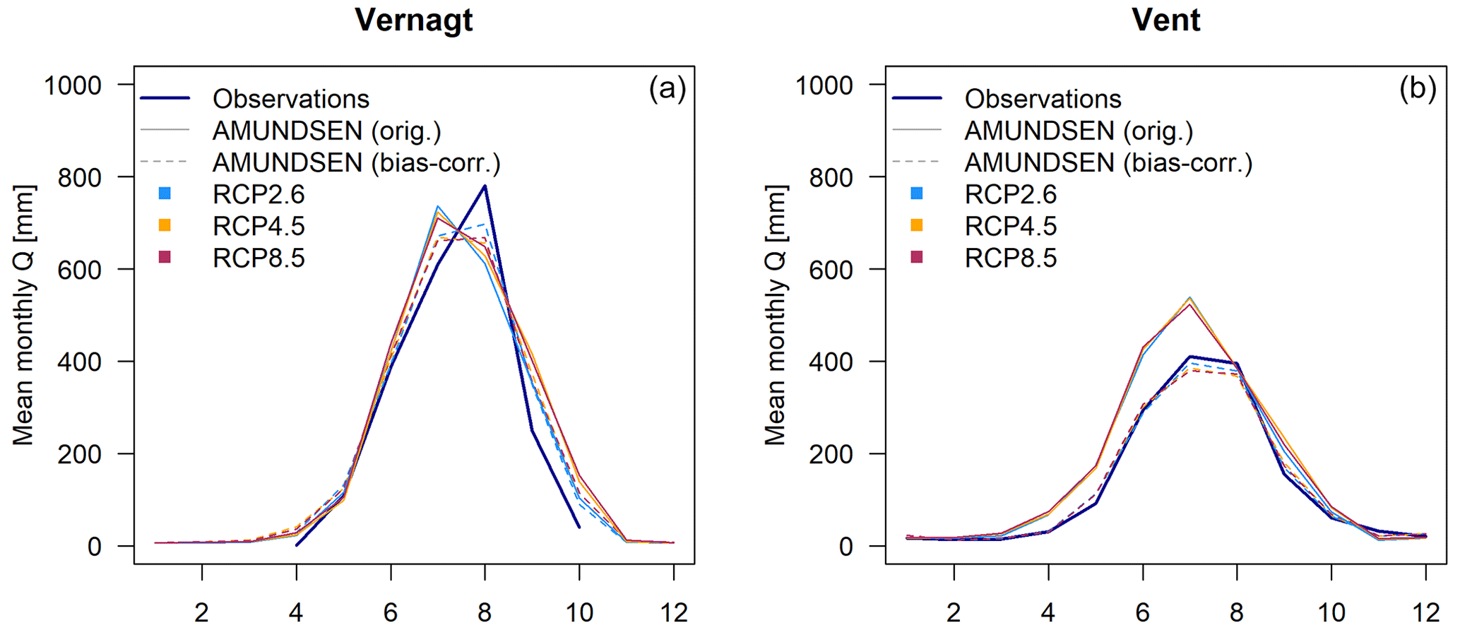
Figure 6Comparison of mean monthly discharge [mm] at gauge Vernagt (a) and Vent (b) derived from measurements, unaltered multi-model means of the original AMUNDSEN output (solid lines) and multi-model means of the bias-corrected AMUNDSEN output (dashed lines) in the overlap period (2007–2020).
3.2 Verification of modeled SSY for the present climate (2007–2020)
We find good agreement between observed and modeled annual SSY at both gauges (Fig. 7), and the Kolmogorov–Smirnov test does not yield significant differences between the observations and model results in mean annual sediment yields. Nevertheless, years with extreme annual yields (both lower and higher) occur in the model results, especially under RCP4.5 and RCP8.5 (e.g., for Vent, max. 3250 t a−1 in RCP4.5 vs. 2120 t a−1 in the observations), likely due to the higher sample size in the projections (42 or 196 years in the projections compared to 14 years in the observations; see also description of Fig. 7).
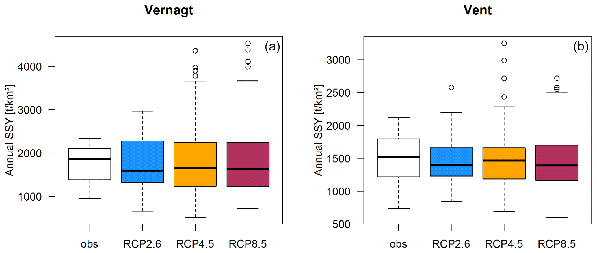
Figure 7Comparison of annual specific SSY in the overlap period (2007–2020) derived from measurements (obs, n=14 years) and QRF modeling results per RCP (n=42 for RCP2.6 and n=196 for RCP4.5 and RCP8.5, respectively) at gauges Vernagt (a) and Vent (b).
Similarly, the seasonality of sediment export is well represented in the overlap period of the projections (Fig. 8), and the Kolmogorov–Smirnov test does not yield significant differences in comparison to the seasonal distribution of the measurements. Monthly SSYs tend to be slightly lower in the projections in August at gauge Vernagt and in July and August at gauge Vent. Similar patterns had already become apparent in the comparison of mean monthly discharges at gauge Vernagt (Fig. 6).
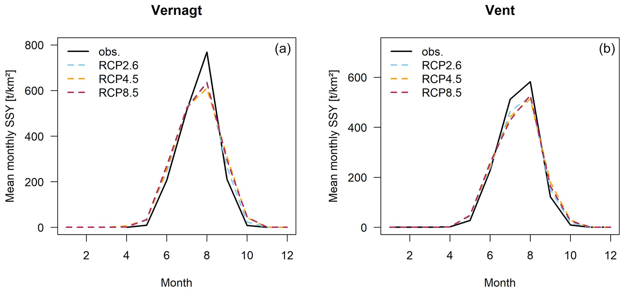
Figure 8Comparison observations (see also Fig. 2) to QRF model forced by climate projections (multi-model means per emission scenario) during the overlap period (2007–2020).
3.3 Assessment of limits of applicability
3.3.1 Out-of-observation-range days
Generally, we find more frequent OOOR days and higher exceedance extents in later time slices and in the higher-emission scenarios (Fig. A1 in the Appendix). At both gauges, OOOR days in Q are relatively rare, but in the higher-emission scenarios and later time slices, OOOR days become more frequent, and individual exceedance extents of more than 100 % occur (Fig. A1 and Table 4). Exceedances in temperature are more frequent at gauge Vernagt, especially under RCP8.5 and after 2040. At gauge Vent, there are only a few OOOR days in T, except under RCP8.5 after 2070.
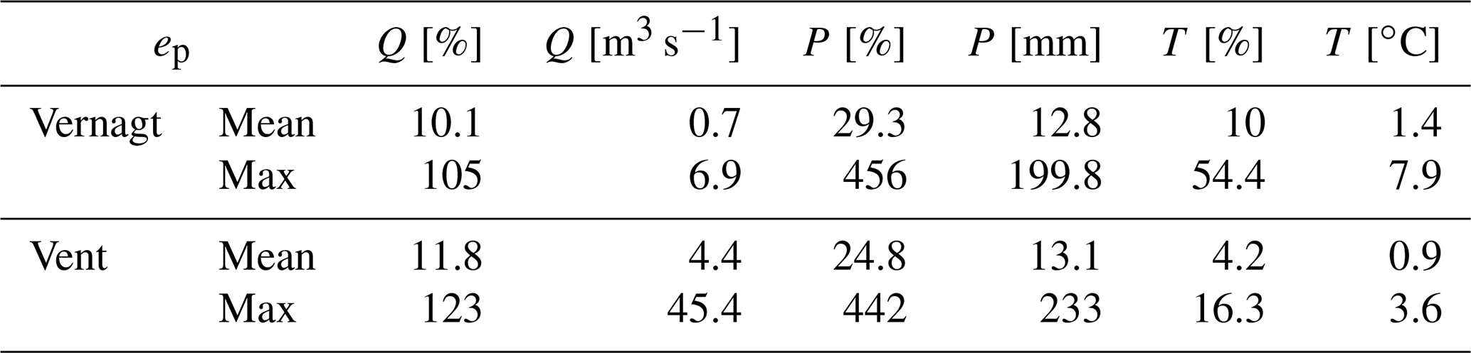
Table 4Mean and maximum exceedance extents ep of the three primary predictors, namely discharge (Q), precipitation (P) and air temperature (T), across all emission scenarios and time slices in percent of the maximum during the training period max(xp,train) and original units.
OOOR data points in summer precipitation are rather rare at both gauges. However, precipitation shows very high exceedance extents of up to ca. 450 % (RCP4.5 after 2070 and RCP8.5 before 2040 at gauge Vent, RCP4.5 after 2070 at gauge Vernagt; Fig. A1 and Table 4). This corresponds to daily precipitation sums of approx. 280 and 240 mm d−1 at gauge Vent and Vernagt, respectively, and is equivalent to over a third of the current mean annual precipitation at gauge Vent (687 mm (Hydrographic Yearbook of Austria, 2016)). Yet, even without the most extreme cases, exceedance extents in precipitation can be quite severe, which corresponds to very heavy precipitation events.
3.3.2 Sensitivity analysis
Figure 9 shows the results of the sensitivity analysis, which indicates the extent to which annual SSY estimates may be affected by underestimations on days with OOOR observations for the different predictors. P is the most sensitive predictor at gauge Vernagt. Yet, although precipitation amounts were altered quite substantially on the 6 d with the highest precipitation in the overlap period (by almost 29 mm; see Table 2), the effect on mean annual SSC is small (≤ 3 %). The same applies to Q, the most sensitive predictor at gauge Vent, which was altered by almost 10 m−3 s−1 on 8 d. Temperature is the second most sensitive parameter at gauge Vernagt, while at gauge Vent, the temperature alterations had little effect on mean annual SSC. At gauge Vent, P is the second most sensitive parameter but with a maximum effect of < 2 % on mean annual SSC.
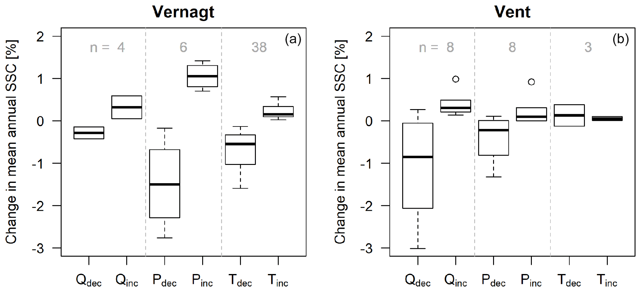
Figure 9Results of the sensitivity analysis for gauges Vernagt (a) and Vent (b) with respect to mean annual SSC of the years with altered days. Subscripts signify an increase (inc) and decrease (dec) in the predictors by the respective average exceedance extent ep,90 and frequency np,90 as identified based on the exceedance analysis. Gray numbers represent the number of altered days in the test data set (2007–2020).
The results of the sensitivity analysis also give an indication of the behavior of the QRF model in response to OOOR data points: as expected, we generally observe a decrease in mean annual SSC if we decrease the predictor values on the selected days (Q, P and T) and vice versa. However, for most predictors, the decrease is more pronounced than the increase (although the same days were altered by the same extent). We presume that this is due to the described incapability of QRF to extrapolate. Thus, we can expect to underestimate the additional effect, e.g., of precipitation exceeding max(Ptrain).
3.3.3 Classification
Table 5 shows that, until 2070, all predictors and RCPs fall within the conditions covered by the sensitivity analysis (with the exception of Q after 2040 at gauge Vent under RCP8.5). This implies that the results of the sensitivity analysis are informative in these cases and that we expect similar or smaller effects of OOOR days on mean annual SSC or SSY in the projection period. After 2070, exceptions occur at both gauges in two out of three RCPs and for several predictors, which implies that the uncertainty is higher than in the results of the sensitivity analysis.
Table 5Results of the classification per emission scenario, predictor and time slice. S denotes more than one-third (italic) and two-thirds (bold, does not occur) of the projections with (assumed in sensitivity); N denotes more than one-third (italic) and two-thirds (bold, does not occur) of the projections with .
The OOOR analysis showed that very high exceedance extents occur in precipitation and that precipitation is a sensitive parameter at both gauges (although the effect on mean annual SSC was small). Additionally, we find that heavy summer precipitation becomes more intense (and only slightly more frequent) (Fig. A2 in Appendix): the 99.5th percentile of the summer precipitation projections increases over time, which suggests that precipitation events become more intense. At the same time, the number of precipitation events that exceed the 99.5th percentile determined from the precipitation observations in the overlap period (2007–2020) hardly increases on average, which suggest that precipitation events of a certain strength do not become (much) more frequent. We also find an increase in daily SSY associated with heavy precipitation events (Fig. A2 in Appendix).
Thus, we additionally assessed whether the trends in annual yields were sensitive to changes in yields on days with OOOR precipitation (Sects. 2.5 and 3.4.1) as extreme precipitation can be very important for sediment dynamics (e.g., by triggering mass movements).
3.4 Projections of future sediment export: changes in annual yields, timing of peak sediment and changes in seasonality
3.4.1 Changes in annual yields and timing of peak sediment
The resulting projections suggest an overall decrease in mean annual SSY for both gauges and each of the three emission scenarios, which is more pronounced at gauge Vernagt (Fig. 10 and Table 6). Accordingly, we consistently find significant negative trends in the projections (2007–2100) in mean annual SSY (Table 6). The differences between the RCPs are small and are smaller than the spread within individual RCPs (Fig. 10). Accordingly, trends in mean annual SSY are only slightly more negative in the high-emission scenarios. With respect to the 99th percentile of annual SSY estimates, trends are less strong than for mean SSY estimates at gauge Vent, while at gauge Vernagt, the trends in the 99th percentile are even stronger than for mean annual SSY estimates.
Table 6Trends in mean and 99th percentile of annual specific SSY projections (2007–2100) given as Sen's slope [t km−2 a−2] for the original estimates and the altered estimates (5-fold-increased SSY on days with OOOR precipitation). Significance levels: * indicates 0.05, indicates 0.01, and indicates 0.001.
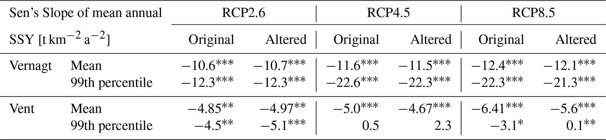
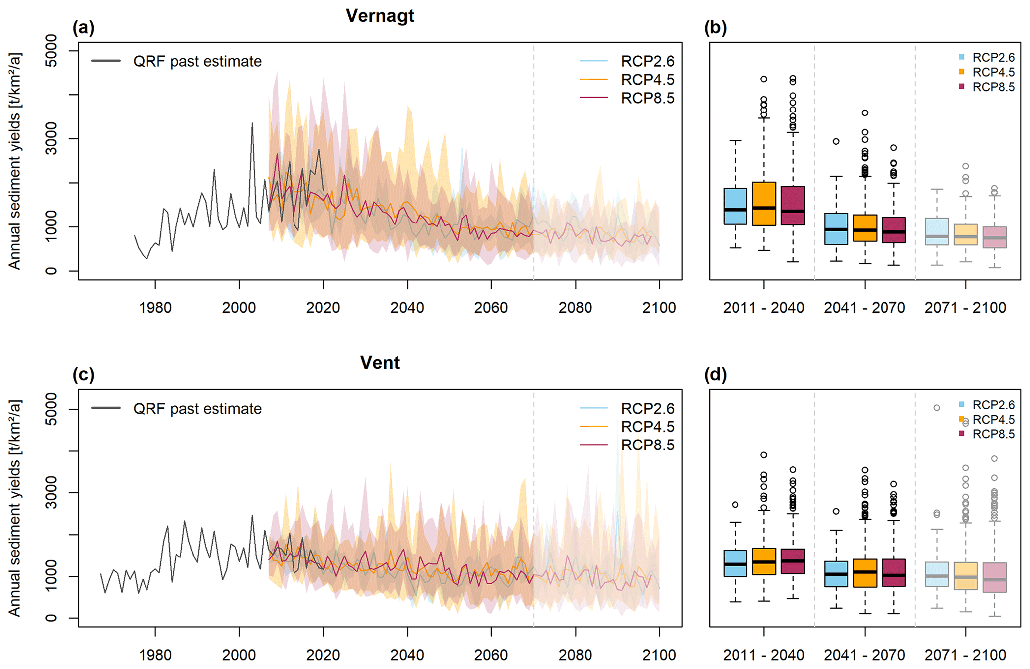
Figure 10(a, c) Mean annual suspended sediment yields per RCP, with the entire range from minima to maxima of the individual projections indicated by the colored envelopes. The period after 2070 is faded due to lower confidence in model results, as pointed out in Sect. 4.3. (b, d) Annual SSY of all respective years and projections within the three time slices.
Negative trends were detected for all individual projections as well: at gauge Vent, 26 (out of 31) are significant (α= 0.05, Sen's slope ranging from −10.8 to −3.8 t km−2 a−2), and at gauge Vernagt, 30 of 31 are significant (α= 0.05, Sen's slope ranging from −15.2 to −6.1 t km−2 a−2).
The trend in the altered time series (with 5-fold-increased daily yields on days with OOOR precipitation; see Sect. 2.5) hardly differs from the trend in the original time series (Table 6). Specifically, at gauge Vernagt, trend characteristics are basically unchanged. The only trend reversal occurs in the 99th percentile at gauge Vent under RCP8.5, where the trend is slightly positive (and significant) instead of negative. We conclude that the overall trend characteristics remain very robust, even if we assume severe underestimation of the model on days with OOOR values in the predictors. Thus, the overall future sediment budget seems to be governed by their mean behavior rather than solitary extreme events.
The synopsis with estimates of annual SSY for the past decades shows that we find increases in annual yields at both gauges up until sometime between 2000 and 2020 and decreases afterwards, which are much more distinct at gauge Vernagt (Figs. 10 and 11). This suggests that peak sediment has already been reached or is underway at both gauges and occurs simultaneously with peak water (Fig. 11).
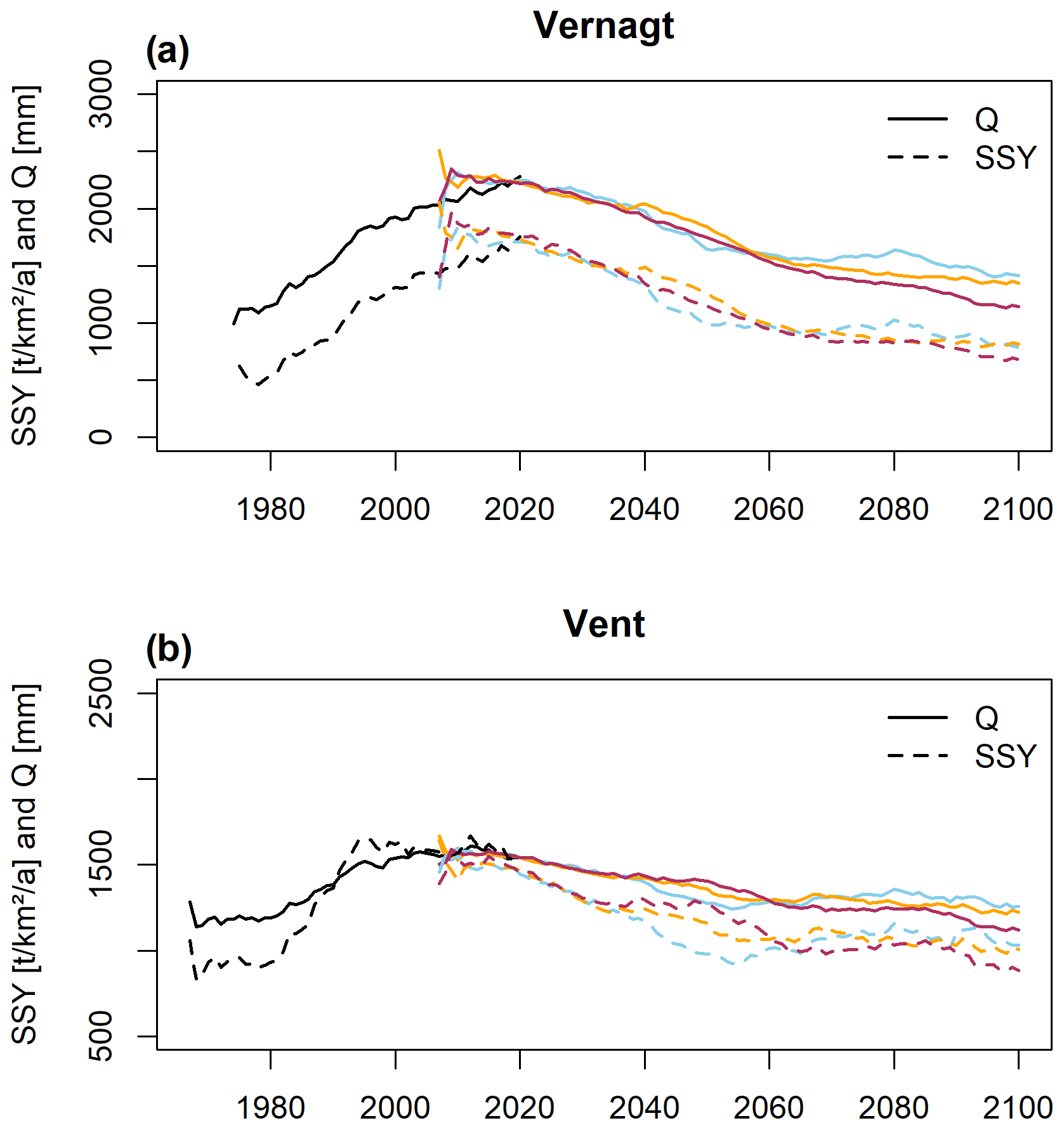
Figure 11Estimated timings of peak water and peak sediment. Black lines indicate past mean annual Q from measurements and mean annual SSY estimates of QRF model; colored lines correspond to different RCPs (compare to Fig. 10). Underlying data have been smoothed using a 15-year moving average.
3.4.2 Changes in seasonality
Mean monthly SSY is projected to decrease substantially during the glacier melt period in August in all RCPs and at both gauges (Fig. 12). As a result, the highest mean monthly SSY shifts from August to July or even to June under RCP8.5 after 2070 at both gauges. Additionally, the spring onset of sediment export is projected to occur at a higher rate and slightly earlier in the year under RCP8.5 after 2070. This represents a decrease in the importance of glacier melt for sediment export. After 2070, only relatively minor further changes are projected under RCP2.6 and RCP4.5, whereas RCP8.5 experiences further decreases in mean monthly SSY throughout the year.
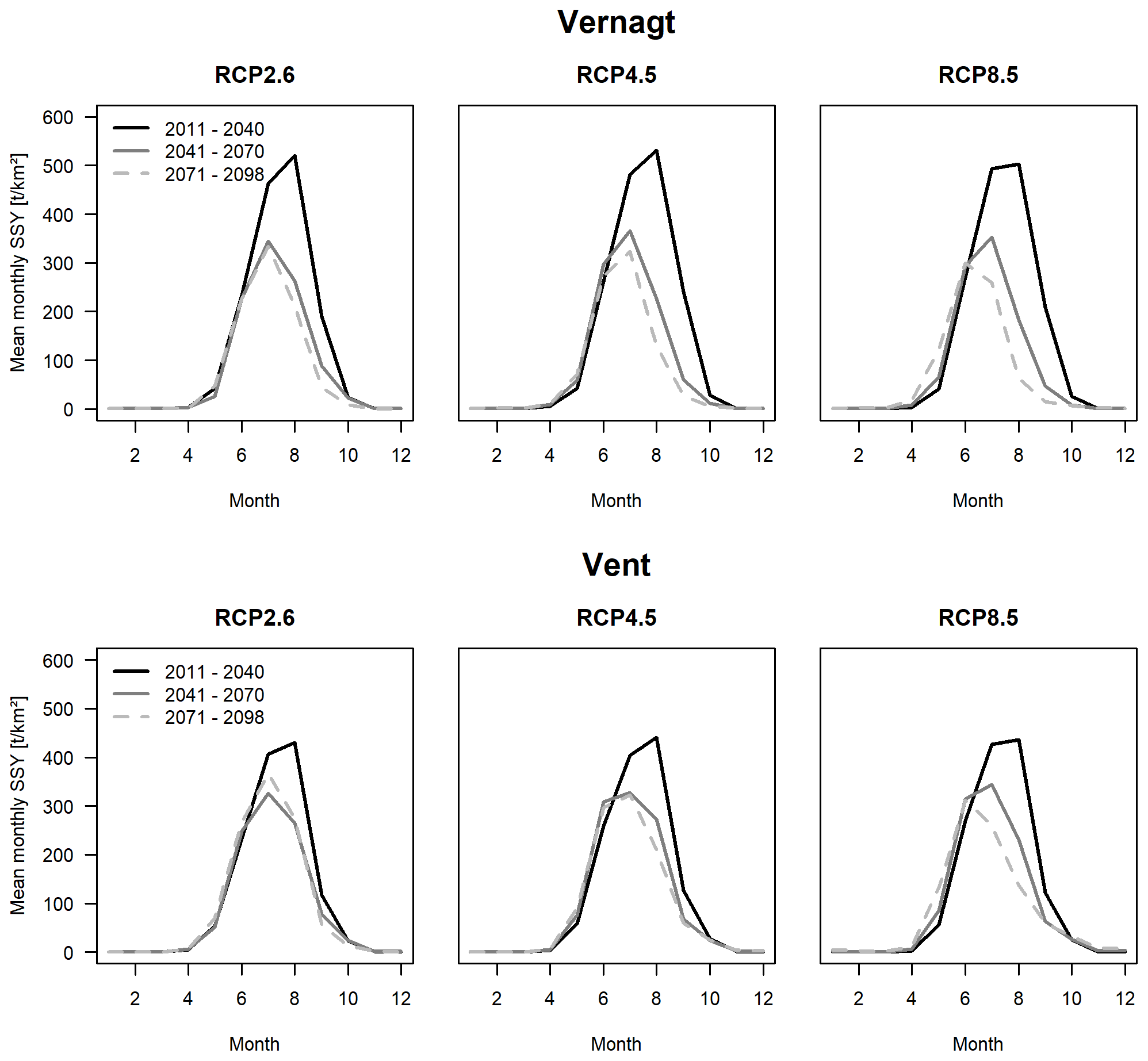
Figure 12Seasonality of mean monthly SSY in three time slices and emission scenarios (as the monthly mean of all respective modeling chains).
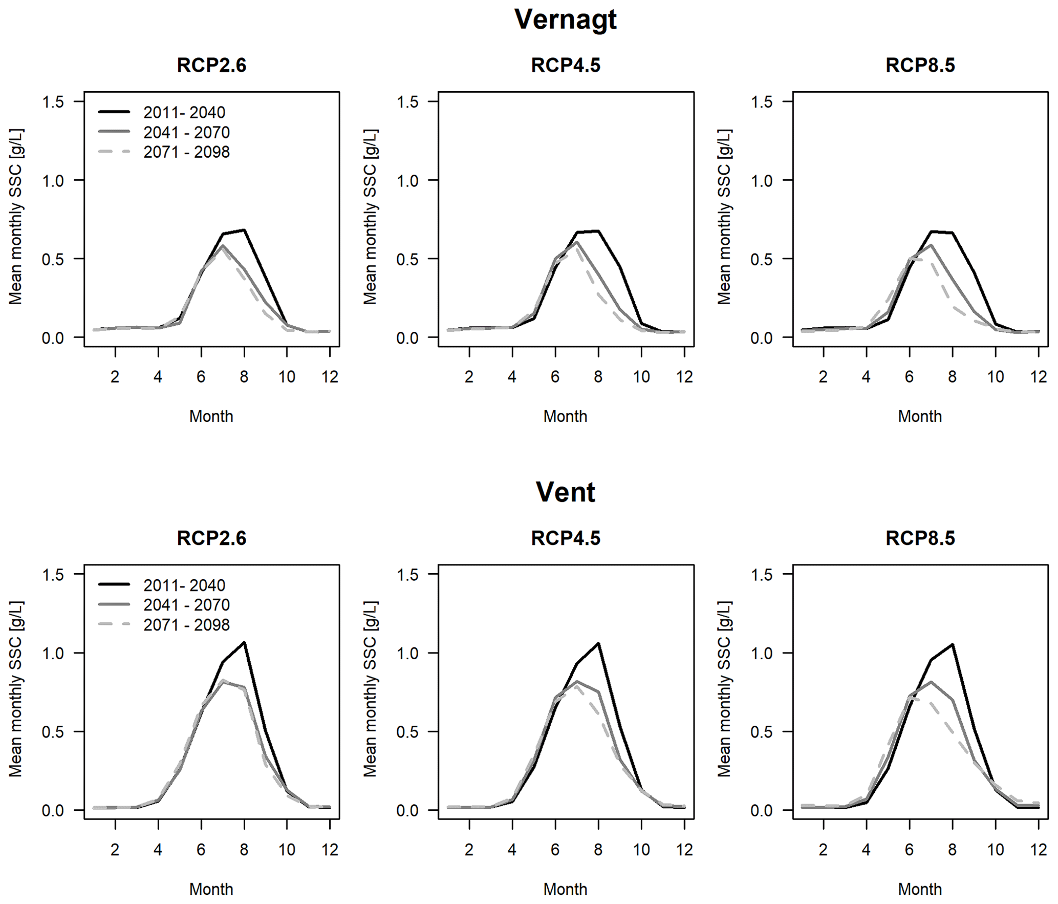
At gauge Vent, a slight increase in mean July SSY is projected after 2070 under RCP2.6. This is likely related to an increase in discharge since this increase is not visible in mean monthly concentrations (Fig. A3 in the Appendix). It also has to be considered that only three projections are averaged for RCP2.6 (as compared to 14 in the other RCPs), which makes it less robust with respect to outliers.
A comparison to the seasonal distributions determined from the altered time series (5-fold-increased SSY on days with OOOR precipitation) showed only very slight differences, which indicates that the seasonal distribution is also insensitive to underestimations of SSY on days with heavy precipitation.
Testing new methods to estimate future suspended sediment export from glacierized high-alpine areas can provide important information, e.g., with regard to flood hazard, sediment or water quality management, since estimating such changes has so far been limited to relatively rough approximations. This study represents the first attempt, to our knowledge, to derive SSY projections using a machine-learning approach and to investigate them in synopsis with reconstructed past SSYs.
4.1 Projected changes in sediment export and location of peak sediment
The presented SSY projections in the Ötzal, Austria, suggest an overall decrease in annual SSY (Fig. 10). This is consistent across emission scenarios (i.e., with respect to the ensemble means), as well as all individual projections (i.e., based on the 31 different RCP–GCM–RCM chains). This is linked to shrinking of glaciers and thus decreases in glacier melt as temperature is projected to increase in all models (between +1.1 (RCP2.6) to +3.8 ∘C (RCP8.5) in the annual mean) (Hanzer et al., 2018). Accordingly, snow cover is projected to decline, especially in low elevations. With respect to precipitation, there is no clear general trend with respect to annual sums; both decreases and increases are projected by individual models (−14 % to +24 %), and multi-model averages are close to zero for all scenarios, yet with a general shift in precipitation from summer to winter
The modeled decrease in SSY is much more distinct at gauge Vernagt, where a trend analysis in the previous study (Schmidt et al., 2023) showed significant positive trends in the period until 2020. At gauge Vent, significant positive trends were detected if all data points since the 1970s were considered (Schmidt et al., 2023). However, if only the years after the distinct increase around 1980 were considered, the trend was slightly negative (Schmidt et al., 2023). This suggests that peak sediment has already been reached or is underway at both gauges and occurs simultaneously with peak water.
These findings match the expectations of conceptual models that sediment yield from deglaciating basins will initially increase (due to increases in glacial erosion, sediment supply accessibility, transport capacity and occurrences of extreme floods) and subsequently decrease as glacier masses decline, meltwater volumes and freeze–thaw weathering decrease, and vegetation colonizes (Antoniazza and Lane, 2021; Zhang et al., 2022). It is expected that peak sediment may lag behind peak meltwater, with a lag that can be up to decades or centuries (Delaney and Adhikari, 2020). This lag is hypothesized to be scale dependent – i.e., it will be shorter for areas closer to the glacierized regions – and to depend on the changes in erosive precipitation: if erosive precipitation decreases, peak sediment occurs simultaneously with peak water, while increasing or stable erosive rainfall scenarios are associated with a lag (Zhang et al., 2022). Indeed, for the study area of this study, a decrease in summer precipitation sums (i.e., June to August, which is the time of minimum snow cover and thus maximum erodibility) is projected (Hanzer et al., 2018). At the same time, heavy precipitation events are projected to become more intense (and only slightly more frequent; see Fig. A2 in the Appendix). However, the negative trend in discharge appears to prevail as our estimates suggest that peak sediment coincides with peak meltwater (Fig. 11).
Sediment export projections differed only slightly (if at all) between emission scenarios; i.e., the spread between projections within one emission scenario is much larger than differences between ensemble means of the three RCPs (Fig. 10). This is due to irreducible internal climate variability, which has been acknowledged in climate modeling (Deser et al., 2012), as well as in erosion modeling (Hirschberg et al., 2021). It should be noted that comparisons to RCP2.6 need to be treated with care as it comprises fewer GCM–RCM combinations (only 3 as compared to 14 in the higher-emission RCPs). Nevertheless, the absence of major differences between RCPs is in accordance with findings by Gobiet and Kotlarski (2020) that “until the middle of the 21st century […] it is projected that climate change in the Alpine area will only slightly depend on the specific emission scenario”. Accordantly, Hanzer et al. (2018) projected glacier volumes to decline by 60 %–65 % until 2050, “largely independent of the emission scenario”.
4.2 Changes in seasonality and response to heavy precipitation events
Despite the overall decrease in SSYs, our results suggest that high annual SSYs are possible, especially at gauge Vent and towards the end of the century (Fig. 10). Additionally, yields on days with heavy precipitation may increase at both gauges – in absolute terms and in relation to the annual export (Fig. A2 in Appendix). This is reasonable, given that increases in heavy precipitation intensity and/or frequency in the European Alps have been detected in measurement data from the past (e.g., Hiebl and Frei, 2018; Scherrer et al., 2016; Gobiet and Kotlarski, 2020), as well as future projections (Gobiet and Kotlarski, 2020; Jacob et al., 2014; Kotlarski et al., 2023) – despite the overall decrease in summer precipitation mentioned above. As a result, we can expect an increase in sediment-related harmful events triggered by heavy precipitation, such as flash floods and gravitational mass movements (i.e., debris flows, landslides) (Huggel et al., 2012; Savi et al., 2020; Gobiet and Kotlarski, 2020). Similar expectations, i.e., increasing high-magnitude transport events in the context of an overall decrease, have e.g., been expressed with respect to bedload in South Tyrol (Coviello et al., 2022). Such a development would have important implications e.g., for sediment management in hydropower production and flood hazard management as the flood risk can increase if cross-sections are reduced after sedimentation, and potential backwater effects need to be considered (Nones, 2019) as much of the damage is associated with transported solids rather than the water itself (Badoux et al., 2014).
Our findings suggest a shift in sediment export seasonality since the highest mean monthly SSY shifts from August to July (or even June) due to substantial reductions in sediment export in July, August and September at both gauges (Fig. 12). This is linked to the projected distinct reductions in glacier melt (Hanzer et al., 2018) and appears to be reasonable given that glacier melt has so far been the dominant transport medium of suspended sediments at these gauges (Schmidt et al., 2023). These results are not sensitive to potential underestimations of SSY on days with very heavy precipitation. Such shifts in seasonality and the concomitant overall reduction in fluvial sediment transport will likely have severe effects on biodiversity, i.e., flora and fauna of glacier-fed streams (Milner et al., 2009, 2017; Gabbud and Lane, 2016; Huss et al., 2017).
4.3 Limitations
As a potential limitation to the presented quantile regression forest approach, out-of-observation-range data points in the predictors can lead to underestimates in SSY on the affected days. Yet, the analysis of such incidents in synopsis with the results of the sensitivity analysis showed that, before 2070, the effect on annual yield estimates is ≤ 3 % Fig. 9). This is very small given the overall high variability in SSC (Vercruysse et al., 2017; Delaney et al., 2018; Schmidt et al., 2023). On a similar note, even assuming rather generous increases in yields on days with OOOR precipitation altered the trends only marginally, which shows that underestimations on individual days with OOOR precipitation have little effect on long-term annual averages. However, we have less confidence in the model results after 2070 for two reasons. First, more frequent and severe OOOR incidents occur during this time, especially in the high-emission scenarios, and fewer projections are covered by the assumptions of the sensitivity analysis. We can therefore expect a higher uncertainty in the model results. Specifically, the effect of underestimation for single large events will aggravate. Second, more than a few glacier simulations suggest that glaciers could have disappeared almost entirely by 2070 (Hanzer et al., 2018), which implies a major shift in the hydro-geomorphic functioning of these catchments. While our QRF models were able to model threshold effects better than sediment rating curves (Schmidt et al., 2023) (likely because they are not bound to linear or monotonous relationships), this is only true for effects that are represented in the training data. Thus, the results for the period after 2070 need to be treated with caution. We have indicated this in the presentation of our results by using transparency or dashed lines instead of solid lines.
As a more general limitation, there are several other factors with the potential to substantially alter and influence sediment dynamics in the study area, which we cannot consider in our models. This concerns geomorphological changes, such as increased paraglacial erosion: debuttressed slopes may trigger landslides and rockfalls, and indeed, increased debris flow and rockfall activity have been shown in response to warming in other areas, likely associated with intensified alpine permafrost thaw (Savi et al., 2020; Hartmeyer et al., 2020; Huggel et al., 2012). Additionally, sediment availability and accessibility increase as erodible landscapes expand (Li et al., 2021a), and subglacial sediment availability might also increase (more subglacial sediment can be accessed by meltwaters as the equilibrium line altitude retreats upslope) until the glacier size becomes smaller than a critical size (Delaney and Adhikari, 2020; Zhang et al., 2022). Although these processes are likely already partially reflected in the observations used for the model training, their intensity may still be too low to be sufficiently learned by the model. Thus, future intensification of these processes could lead to higher sediment export rates than our estimates suggest and might thereby affect the estimated location of peak sediment. Notwithstanding, there are also several factors that could lead to decreases in sediment export, such as decreases in connectivity (such as the formation of supra-, sub- or proglacial lakes or outwash fans which act as sediment traps) or decreasing glacial erosion as glaciers recede (Zhang et al., 2022). Additionally, freeze–thaw weathering may decrease (Hirschberg et al., 2021), and it is not clear how quickly the deglaciating landscapes will stabilize, e.g., through eluviation of fine materials and fluvial sorting of sediment, which progressively increases the resistance to entrainment and transport (Ballantyne, 2002; Lane et al., 2017), or vegetation colonization (Haselberger et al., 2021; Altmann et al., 2023; Musso et al., 2020; Eichel et al., 2018). Many of these processes are ultimately governed by temperature and/or precipitation, and we have chosen the predictors to act as proxies (e.g., antecedent moisture and temperature conditions could be crucial for mass movements). While this is out of the scope of the presented study, we encourage future studies to work towards including more advanced proxies for geomorphological changes.
4.4 Uncertainties
The presented results are associated with uncertainties, which are a combination of uncertainties inherited from the underlying climatological and hydrological projections and uncertainties inherent in the QRF approach. Climate model uncertainty represents a combination of uncertainties in assumptions of future anthropogenic greenhouse gas emission, GCM uncertainty (different GCMs produce different responses to the same radiative forcing) and RCM uncertainty (different RCMs forced by same the GCM produce different regional responses) (Evin et al., 2021; Gobiet et al., 2014). It has been found that EURO-CORDEX simulations may be biased towards “too cold, too wet, too windy”, but these uncertainties are mostly within the observational uncertainties, and simulations “reproduce fairly well the recent past climate despite some biases” (Vautard et al., 2021). To address this, it was recommended to carry out bias correction, which has been performed by means of quantile mapping for the precipitation and temperature projections (Hanzer et al., 2018). The hydrological model results are also associated with uncertainties, such as the tendency to overestimate spring runoff, winter snow accumulation and glacier mass balances. We have addressed this through bias correcting the discharge projections, which resulted in a more adequate representation of discharge seasonality and volumes. Certainly, bias correction methods such as quantile mapping in turn introduce uncertainties, e.g., by assuming that the biases are stationary, i.e., do not change over time (Gudmundsson et al., 2012). Hydrological simulations that do not show the necessity for this correction could eliminate this issue. Uncertainties in the QRF approach have been addressed in a previous study and include the tendency to underestimate rare, high-magnitude daily SSYs (albeit with small effects on the respective annual yields); the underestimations on days with OOOR values (which had small effects until 2070, as discussed in detail above); and the choice of temporal resolution (i.e., daily compared to hourly resolution involves some loss of information, e.g., on precipitation intensities, but the effect was also found to be small) (Schmidt et al., 2023). Since QRF is a data-driven approach, the quality of the estimates hinges on the underlying training data set, as well as the choice of predictors, i.e., a large and varied enough data set in combination with predictors that meaningfully represent the most important processes improves the quality of the estimates (Schmidt et al., 2023). Thus, future studies are recommended to explicitly sample extreme events and/or verify the representativity of the training data set.
We found decreasing trends in annual SSY at both gauges regardless of the emission scenario, which suggests that peak sediment was already reached between 2000 and 2020. This is linked to substantial decreases in discharge volumes, especially during the glacier melt phase in late summer, as glaciers continue to melt as a result of increasing temperatures. These findings persist even if yields on days with projected heavy precipitation are inflated by a factor of 5. Despite the projected overall decrease, high(er) annual yields are possible, likely in response to heavy summer precipitation, which could become more intense according to the projections. This discrepancy has important implications for sediment management but also e.g., for flood management.
To our knowledge, this study represents the first attempt to combine machine learning for suspended sediment modeling with climate and hydrological projections in order to derive projections of sediment export in high-alpine areas. It demonstrated that a quantile regression forest can be a valuable tool for this application. We addressed known issues of the QRF, i.e., underestimations on days where predictors in the projection period exceed the range represented in the training data. The influence of such underestimations on the results were shown to be negligible until 2070. We conclude that the presented results are much more uncertain after 2070, partly because of more frequent and severe out-of-observation-range data points, but mainly since a major shift in the functioning of the hydro-geomorphic system can be expected as deglaciation is quasi completed.
However, while the chosen predictors represent proxies for crucial processes controlling sediment transport in these high-alpine environments, several potentially crucial geomorphological factors that could increase or decrease sediment export (and thereby change the projected trends and location of peak sediment) could not be taken into account. These include increases in rockfalls and landsliding, changes in connectivity, or vegetation colonization. Future studies are encouraged to include these factors more explicitly.
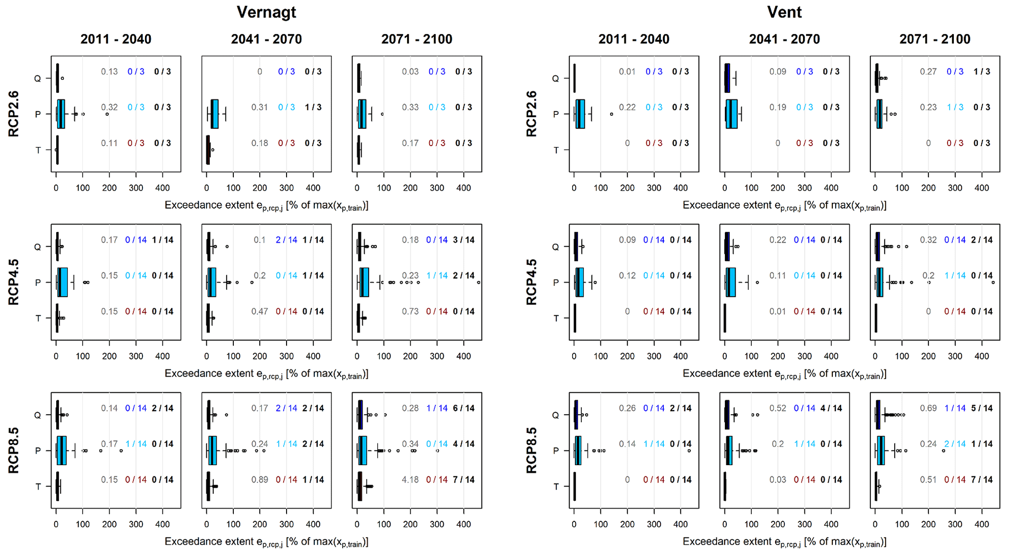
Figure A1Results of the classification based on the sensitivity and OOOR analyses. The boxplots show the distribution of exceedance extents for each RCP and predictor on all days j within the respective time slice ts. Gray numbers denote the average of all projections within the respective RCP, time slice and predictor. Colored numbers indicate the number of projections with mean exceedance extent (as used for the sensitivity analysis). Black numbers indicate the number or projections with the mean number of OOOR days per year (as used for the sensitivity analysis).
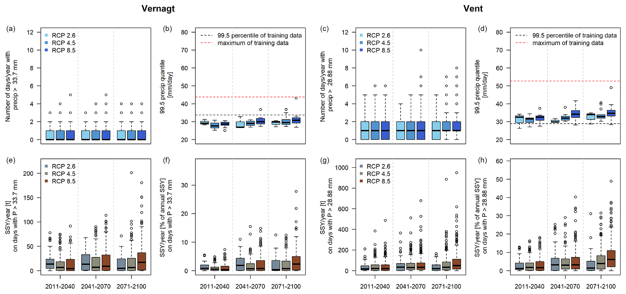
Figure A2Analysis of summer precipitation projections (a–d) and SSY projections (e–h) at gauges Vernagt and Vent. (a, c) Frequency of days with heavy summer precipitation (> 99.5th percentile of the training data, i.e., 33.7 mm d−1, Vernagt, and 28.88 mm d−1, Vent). (b, d) Intensity of heavy summer precipitation events over time, expressed as the 99.5th percentile. (e, g) Sediment export on days with precipitation > 99.5th percentile of the training data. (f, h) Sediment export on days with precipitation > 99.5th percentile of the training data relative to the respective annual yields.
The model code, input data and results are published under DOI https://doi.org/10.23728/b2share.5f706863fc5041c49cb8d1a8cd55f613 (Grosse et al., 2023).
LKS developed the general idea and conceptualized the study with TF and PG, with the mentoring and reviewing of AB. LKS requested the necessary input data, PG adapted and extended the model code under the supervision of TF and LKS, and PG and LKS performed the model runs. LKS developed and conducted the analysis of model limitations and conducted the statistical analyses with support and supervision by TF. LKS prepared the original draft of the paper, including all the figures, and all the authors contributed to writing this paper.
The contact author has declared that none of the authors has any competing interests.
Publisher's note: Copernicus Publications remains neutral with regard to jurisdictional claims made in the text, published maps, institutional affiliations, or any other geographical representation in this paper. While Copernicus Publications makes every effort to include appropriate place names, the final responsibility lies with the authors.
The authors would like to thank Florian Hanzer and Ulrich Strasser for providing the projections required as input data for this study. We thank the Hydrographic Service of Tyrol, Austria, and the Bavarian Academy of Sciences and Humanities for the provision of data, as well as the logistical support. We thank Marvin Teschner for his support in the data analyses. We would like to thank Mustafa Al-Mukhtar, Ting Zhang and an anonymous referee for their constructive and detailed comments that helped to improve this paper.
This research was supported by the Deutsche Forschungsgemeinschaft, as part of the Research Training Group “Natural Hazards and Risks in a Changing World” (grant nos. NatRiskChange GRK 2043/1 and GRK 2043/2) and by a fieldwork fellowship of the German Hydrological Society (DHG).
This paper was edited by Manuela Irene Brunner and reviewed by Ting Zhang, Mustafa Al-Mukhtar, and one anonymous referee.
Abermann, J., Lambrecht, A., Fischer, A., and Kuhn, M.: Quantifying changes and trends in glacier area and volume in the Austrian Ötztal Alps (1969-1997-2006), The Cryosphere, 3, 205–215, https://doi.org/10.5194/tc-3-205-2009, 2009.
Al-Mukhtar, M.: Random forest, support vector machine, and neural networks to modelling suspended sediment in Tigris River-Baghdad, Environ. Monit. Assess., 191, 673, https://doi.org/10.1007/s10661-019-7821-5, 2019.
Altmann, M., Ramskogler, K., Mikolka-Flöry, S., Pfeiffer, M., Haas, F., Heckmann, T., Rom, J., Fleischer, F., Himmelstoß, T., Pfeifer, N., Ressl, C., Tasser, E., and Becht, M.: Quantitative Long-Term Monitoring (1890–2020) of Morphodynamic and Land-Cover Changes of a LIA Lateral Moraine Section, Geosciences, 13, 95, https://doi.org/10.3390/geosciences13040095, 2023.
Antoniazza, G. and Lane, S. N.: Sediment yield over glacial cycles: A conceptual model, Prog. Phys. Geog.., 58, 842–865, https://doi.org/10.1177/0309133321997292, 2021.
Badoux, A., Andres, N., and Turowski, J. M.: Damage costs due to bedload transport processes in Switzerland, Nat. Hazards Earth Syst. Sci., 14, 279–294, https://doi.org/10.5194/nhess-14-279-2014, 2014.
Ballantyne, C. K.: Paraglacial geomorphology, Quaternary Sci. Rev., 21, 1935–2017, https://doi.org/10.1016/S0277-3791(02)00005-7, 2002.
Beniston, M., Farinotti, D., Stoffel, M., Andreassen, L. M., Coppola, E., Eckert, N., Fantini, A., Giacona, F., Hauck, C., Huss, M., Huwald, H., Lehning, M., López-Moreno, J.-I., Magnusson, J., Marty, C., Morán-Tejéda, E., Morin, S., Naaim, M., Provenzale, A., Rabatel, A., Six, D., Stötter, J., Strasser, U., Terzago, S., and Vincent, C.: The European mountain cryosphere: a review of its current state, trends, and future challenges, The Cryosphere, 12, 759–794, https://doi.org/10.5194/tc-12-759-2018, 2018.
Bilotta, G. S. and Brazier, R. E.: Understanding the influence of suspended solids on water quality and aquatic biota, Water Res., 42, 2849–2861, https://doi.org/10.1016/j.watres.2008.03.018, 2008.
Bogen, J.: The impact of climate change on glacial sediment delivery to rivers, in: Sediment Dynamics in Changing Environments, Proceedings of a symposium held in Christchurch, New Zealand, December 2008, IAHS Publ., 325, 432–439, 2008.
Bolibar, J., Rabatel, A., Gouttevin, I., Zekollari, H., and Galiez, C.: Nonlinear sensitivity of glacier mass balance to future climate change unveiled by deep learning, Nat. Commun., 13, 409, https://doi.org/10.1038/s41467-022-28033-0, 2022.
Braun, L. N., Escher-Vetter, H., Siebers, M., and Weber, M.: Water Balance of the highly Glaciated Vernagt Basin, Ötztal Alps, in: The water balance of the alps: what do we need to protect the water resources of the Alps? Proceedings of the conference held at Innsbruck university, 28–29 September 2006, 33–42, https://diglib.uibk.ac.at/ulbdok/content/pageview/268995 (last access: 8 May 2023), 2007.
Buckel, J. and Otto, J.-C.: The Austrian Glacier Inventory GI 4 (2015) in ArcGis (shapefile) format, PANGAEA [data set], https://doi.org/10.1594/PANGAEA.887415, 2018.
Campforts, B., Shobe, C. M., Overeem, I., and Tucker, G. E.: The Art of Landslides: How Stochastic Mass Wasting Shapes Topography and Influences Landscape Dynamics, J. Geophys. Res.-Earth, 127, e2022JF006745, https://doi.org/10.1029/2022JF006745, 2022.
Carrivick, J. L. and Heckmann, T.: Short-term geomorphological evolution of proglacial systems, Geomorphology, 287, 3–28, https://doi.org/10.1016/j.geomorph.2017.01.037, 2017.
Carrivick, J. L. and Tweed, F. S.: Deglaciation controls on sediment yield: Towards capturing spatio-temporal variability, Earth-Sci. Rev., 221, 103809, https://doi.org/10.1016/j.earscirev.2021.103809, 2021.
Cohen, S., Kettner, A. J., Syvitski, J. P. M., and Fekete, B. M.: WBMsed, a distributed global-scale riverine sediment flux model: Model description and validation, Comput. Geosci., 53, 80–93, https://doi.org/10.1016/j.cageo.2011.08.011, 2013.
Costa, A., Anghileri, D., and Molnar, P.: Hydroclimatic control on suspended sediment dynamics of a regulated Alpine catchment: a conceptual approach, Hydrol. Earth Syst. Sci., 22, 3421–3434, https://doi.org/10.5194/hess-22-3421-2018, 2018.
Coviello, V., Vignoli, G., Simoni, S., Bertoldi, W., Engel, M., Buter, A., Marchetti, G., Andreoli, A., Savi, S., and Comiti, F.: Bedload Fluxes in a Glacier-Fed River at Multiple Temporal Scales, Water Resour. Res., 58, e2021WR031873, https://doi.org/10.1029/2021WR031873, 2022.
Delaney, I. and Adhikari, S.: Increased Subglacial Sediment Discharge in a Warming Climate: Consideration of Ice Dynamics, Glacial Erosion, and Fluvial Sediment Transport, Geophys. Res. Lett., 47, e2019GL085672, https://doi.org/10.1029/2019GL085672, 2020.
Delaney, I., Bauder, A., Werder, M., and Farinotti, D.: Regional and annual variability in subglacial sediment transport by water for two glaciers in the Swiss Alps, Front. Earth Sci., 6, 175, https://doi.org/10.3929/ethz-b-000305762, 2018.
Delaney, I., Werder, M. A., and Farinotti, D.: A Numerical Model for Fluvial Transport of Subglacial Sediment, J. Geophys. Res.-Earth, 124, 2197–2223, https://doi.org/10.1029/2019JF005004, 2019.
Delaney, I., Anderson, L., and Herman, F.: Modeling the spatially distributed nature of subglacial sediment transport and erosion, Earth Surf. Dynam., 11, 663–680, https://doi.org/10.5194/esurf-11-663-2023, 2023.
Deser, C., Phillips, A., Bourdette, V., and Teng, H.: Uncertainty in climate change projections: the role of internal variability, Clim. Dynam., 38, 527–546, https://doi.org/10.1007/s00382-010-0977-x, 2012.
Eichel, J., Draebing, D., and Meyer, N.: From active to stable: Paraglacial transition of Alpine lateral moraine slopes, Land Degrad. Dev., 29, 4158–4172, https://doi.org/10.1002/ldr.3140, 2018.
Escher-Vetter, H.: Climate change information as derived from long-term measurements of winter and summer mass balance, in: Extended Abstracts, 29th International Conference on Alpine Meteorology, Chambéry, France, 4–8 June 2007, 465–468, https://citeseerx.ist.psu.edu/document?repid=rep1&type=pdf&doi=04eeeb26130819e9d8183bc3150db19837c401bd (last access: 22 December 2023), 2007.
Evin, G., Somot, S., and Hingray, B.: Balanced estimate and uncertainty assessment of European climate change using the large EURO-CORDEX regional climate model ensemble, Earth Syst. Dynam., 12, 1543–1569, https://doi.org/10.5194/esd-12-1543-2021, 2021.
Francke, T., López-Tarazón, J. A., and Schröder, B.: Estimation of suspended sediment concentration and yield using linear models, random forests and quantile regression forests, Hydrol. Process., 22, 4892–4904, https://doi.org/10.1002/hyp.7110, 2008a.
Francke, T., López-Tarazón, J. A., Vericat, D., Bronstert, A., and Batalla, R. J.: Flood-based analysis of high-magnitude sediment transport using a non-parametric method, Earth Surf. Proc. Land., 33, 2064–2077, https://doi.org/10.1002/esp.1654, 2008b.
Gabbud, C. and Lane, S. N.: Ecosystem impacts of Alpine water intakes for hydropower: the challenge of sediment management, WIRES Water, 3, 41–61, https://doi.org/10.1002/wat2.1124, 2016.
Gobiet, A. and Kotlarski, S.: Future Climate Change in the European Alps, edited by: Gobiet, A. and Kotlarski, S., Oxford research encyclopedia of climate science, Oxford University Press, https://doi.org/10.1093/acrefore/9780190228620.013.767, 2020.
Gobiet, A., Kotlarski, S., Beniston, M., Heinrich, G., Rajczak, J., and Stoffel, M.: 21st century climate change in the European Alps – A review, Sci. Total Environ., 493, 1138–1151, https://doi.org/10.1016/j.scitotenv.2013.07.050, 2014.
Grosse, P. M., Schmidt, L. K., Francke, T., Hanzer, F., and Strasser, U.: A quantile regression forest approach to model future sediment export from two high alpine catchments based on climate and hydrologic projections, B2Share [data set], https://doi.org/10.23728/b2share.5f706863fc5041c49cb8d1a8cd55f613, 2023.
Gudmundsson, L.: qmap: Statistical transformations for post-processing climate model output, R package version 1.0-4, R-project [code], https://CRAN.R-project.org/package=qmap (last access: 18 May 2023), 2016.
Gudmundsson, L., Bremnes, J. B., Haugen, J. E., and Engen-Skaugen, T.: Technical Note: Downscaling RCM precipitation to the station scale using statistical transformations – a comparison of methods, Hydrol. Earth Syst. Sci., 16, 3383–3390, https://doi.org/10.5194/hess-16-3383-2012, 2012.
Guillén-Ludeña, S., Manso, P. A., and Schleiss, A. J.: Multidecadal Sediment Balance Modelling of a Cascade of Alpine Reservoirs and Perspectives Based on Climate Warming, Water, 10, 1759, https://doi.org/10.3390/w10121759, 2018.
Gupta, D., Hazarika, B. B., Berlin, M., Sharma, U. M., and Mishra, K.: Artificial intelligence for suspended sediment load prediction: a review, Environ. Earth Sci., 80, 346, https://doi.org/10.1007/s12665-021-09625-3, 2021.
Hanus, S., Hrachowitz, M., Zekollari, H., Schoups, G., Vizcaino, M., and Kaitna, R.: Future changes in annual, seasonal and monthly runoff signatures in contrasting Alpine catchments in Austria, Hydrol. Earth Syst. Sci., 25, 3429–3453, https://doi.org/10.5194/hess-25-3429-2021, 2021.
Hanzer, F., Helfricht, K., Marke, T., and Strasser, U.: Multilevel spatiotemporal validation of snow/ice mass balance and runoff modeling in glacierized catchments, The Cryosphere, 10, 1859–1881, https://doi.org/10.5194/tc-10-1859-2016, 2016.
Hanzer, F., Förster, K., Nemec, J., and Strasser, U.: Projected cryospheric and hydrological impacts of 21st century climate change in the Ötztal Alps (Austria) simulated using a physically based approach, Hydrol. Earth Syst. Sci., 22, 1593–1614, https://doi.org/10.5194/hess-22-1593-2018, 2018.
Hartmeyer, I., Delleske, R., Keuschnig, M., Krautblatter, M., Lang, A., Schrott, L., and Otto, J.-C.: Current glacier recession causes significant rockfall increase: the immediate paraglacial response of deglaciating cirque walls, Earth Surf. Dynam., 8, 729–751, https://doi.org/10.5194/esurf-8-729-2020, 2020.
Haselberger, S., Ohler, L.-M., Junker, R. R., Otto, J.-C., Glade, T., and Kraushaar, S.: Quantification of biogeomorphic interactions between small-scale sediment transport and primary vegetation succession on proglacial slopes of the Gepatschferner, Austria, Earth Surf. Proc. Land., 46, 1941–1952, https://doi.org/10.1002/esp.5136, 2021.
Hiebl, J. and Frei, C.: Daily precipitation grids for Austria since 1961 – development and evaluation of a spatial dataset for hydroclimatic monitoring and modelling, Theor. Appl. Climatol., 132, 327–345, https://doi.org/10.1007/s00704-017-2093-x, 2018.
Hinderer, M., Kastowski, M., Kamelger, A., Bartolini, C., and Schlunegger, F.: River loads and modern denudation of the Alps – A review, Earth-Sci. Rev., 118, 11–44, https://doi.org/10.1016/j.earscirev.2013.01.001, 2013.
Hirschberg, J., Fatichi, S., Bennett, G. L., McArdell, B. W., Peleg, N., Lane, S. N., Schlunegger, F., and Molnar, P.: Climate Change Impacts on Sediment Yield and Debris-Flow Activity in an Alpine Catchment, J. Geophys. Res.-Earth, 126, e2020JF005739, https://doi.org/10.1029/2020JF005739, 2021.
Huggel, C., Clague, J. J., and Korup, O.: Is climate change responsible for changing landslide activity in high mountains?, Earth Surf. Proc. Land., 37, 77–91, https://doi.org/10.1002/esp.2223, 2012.
Huss, M.: Present and future contribution of glacier storage change to runoff from macroscale drainage basins in Europe, Water Resour. Res., 47, W07511, https://doi.org/10.1029/2010WR010299, 2011.
Huss, M. and Hock, R.: Global-scale hydrological response to future glacier mass loss, Nat. Clim. Change, 8, 135–140, https://doi.org/10.1038/s41558-017-0049-x, 2018.
Huss, M., Bookhagen, B., Huggel, C., Jacobsen, D., Bradley, R. S., Clague, J. J., Vuille, M., Buytaert, W., Cayan, D. R., Greenwood, G., Mark, B. G., Milner, A. M., Weingartner, R., and Winder, M.: Toward mountains without permanent snow and ice, Earths Future, 5, 418–435, https://doi.org/10.1002/2016EF000514, 2017.
Hydrographic yearbook of Austria: Hydrographisches Jahrbuch von Österreich, Hydrographischer Dienst in Österreich, Bundesministerium für Land- und Forstwirtschaft, Umwelt und Wasserwirtschaft Abteilung VII/3, https://wasser.umweltbundesamt.at/ hydjb/ (last access: 8 May 2023), 2016.
Iverson, R. M. and George, D. L.: A depth-averaged debris-flow model that includes the effects of evolving dilatancy. I. Physical basis, P. Roy. Soc. A-Math. Phy., 470, 20130819, https://doi.org/10.1098/rspa.2013.0819, 2014.
Jacob, D., Petersen, J., Eggert, B., Alias, A., Christensen, O. B., Bouwer, L. M., Braun, A., Colette, A., Déqué, M., Georgievski, G., Georgopoulou, E., Gobiet, A., Menut, L., Nikulin, G., Haensler, A., Hempelmann, N., Jones, C., Keuler, K., Kovats, S., Kröner, N., Kotlarski, S., Kriegsmann, A., Martin, E., van Meijgaard, E., Moseley, C., Pfeifer, S., Preuschmann, S., Radermacher, C., Radtke, K., Rechid, D., Rounsevell, M., Samuelsson, P., Somot, S., Soussana, J.-F., Teichmann, C., Valentini, R., Vautard, R., Weber, B., and Yiou, P.: EURO-CORDEX: new high-resolution climate change projections for European impact research, Reg. Environ. Change, 14, 563–578, https://doi.org/10.1007/s10113-013-0499-2, 2014.
Jimeno-Sáez, P., Martínez-España, R., Casalí, J., Pérez-Sánchez, J., and Senent-Aparicio, J.: A comparison of performance of SWAT and machine learning models for predicting sediment load in a forested Basin, Northern Spain, Catena, 212, 105953, https://doi.org/10.1016/j.catena.2021.105953, 2022.
Kotlarski, S., Gobiet, A., Morin, S., Olefs, M., Rajczak, J., and Samacoïts, R.: 21st Century alpine climate change, Clim. Dynam., 60, 65–86, https://doi.org/10.1007/s00382-022-06303-3, 2023.
Kuhn, M., Helfricht, K., Ortner, M., Landmann, J., and Gurgiser, W.: Liquid water storage in snow and ice in 86 Eastern Alpine basins and its changes from 1970–97 to 1998–2006, Ann. Glaciol., 57, 11–18, https://doi.org/10.1017/aog.2016.24, 2016.
Lalk, P., Haimann, M., and Habersack, H.: Monitoring, Analyse und Interpretation des Schwebstofftransportes an österreichischen Flüssen, Österr. Wasser-Abfallwirtsch., 66, 306–315, https://doi.org/10.1007/s00506-014-0175-x, 2014.
Land Tirol: Digital terrain model of Tyrol, 10m resolution, EPSG 31254, data.gv.at [data set], https://www.data.gv.at/katalog/dataset/land-tirol_tirolgelnde (last access: 8 May 2023), 2016.
Land Tirol: tiris OGD map service “Wasser”, data.gv.at [data set], https://www.data.gv.at/katalog/dataset/0b5d6529-d88c-46c0-84f7-b37282e96ce8 (last access: 5 July 2021), 2021.
Landers, M. N. and Sturm, T. W.: Hysteresis in suspended sediment to turbidity relations due to changing particle size distributions: Hysteresis Suspended Sediment-Turbidity With Particle Size, Water Resour. Res., 49, 5487–5500, https://doi.org/10.1002/wrcr.20394, 2013.
Lane, S. N., Bakker, M., Gabbud, C., Micheletti, N., and Saugy, J.-N.: Sediment export, transient landscape response and catchment-scale connectivity following rapid climate warming and Alpine glacier recession, Geomorphology, 277, 210–227, https://doi.org/10.1016/j.geomorph.2016.02.015, 2017.
Lane, S. N., Bakker, M., Costa, A., Girardclos, S., Loizeau, J.-L., Molnar, P., Silva, T., Stutenbecker, L., and Schlunegger, F.: Making stratigraphy in the Anthropocene: climate change impacts and economic conditions controlling the supply of sediment to Lake Geneva, Sci. Rep., 9, 8904, https://doi.org/10.1038/s41598-019-44914-9, 2019.
Lantz, B.: Machine Learning with R: Expert techniques for predictive modeling, 3rd edn., Packt Publishing Ltd, 459 pp., ISBN 978-1-78829-155-2, 2019.
Li, D., Li, Z., Zhou, Y., and Lu, X. X.: Substantial Increases in the Water and Sediment Fluxes in the Headwater Region of the Tibetan Plateau in Response to Global Warming, Geophys. Res. Lett., 47, e2020GL087745, https://doi.org/10.1029/2020GL087745, 2020.
Li, D., Overeem, I., Kettner, A., Zhou, Y., and Xixi, L.: Air Temperature Regulates Erodible Landscape, Water, and Sediment Fluxes in the Permafrost-Dominated Catchment on the Tibetan Plateau, Water Resour. Res., 57, e2020WR028193, https://doi.org/10.1029/2020WR028193, 2021a.
Li, D., Lu, X., Overeem, I., Walling, D. E., Syvitski, J., Kettner, A. J., Bookhagen, B., Zhou, Y., and Zhang, T.: Exceptional increases in fluvial sediment fluxes in a warmer and wetter High Mountain Asia, Science, 374, 599–603, https://doi.org/10.1126/science.abi9649, 2021b.
Li, D., Lu, X., Walling, D. E., Zhang, T., Steiner, J. F., Wasson, R. J., Harrison, S., Nepal, S., Nie, Y., Immerzeel, W. W., Shugar, D. H., Koppes, M., Lane, S., Zeng, Z., Sun, X., Yegorov, A., and Bolch, T.: High Mountain Asia hydropower systems threatened by climate-driven landscape instability, Nat. Geosci., 15, 520–530, https://doi.org/10.1038/s41561-022-00953-y, 2022.
Madsen, H., Lawrence, D., Lang, M., Martinkova, M., and Kjeldsen, T. R.: Review of trend analysis and climate change projections of extreme precipitation and floods in Europe, J. Hydrol., 519, 3634–3650, https://doi.org/10.1016/j.jhydrol.2014.11.003, 2014.
Meinshausen, N.: Quantile Regression Forests, J. Mach. Learn. Res., 7, 983–999, 2006.
Micheletti, N. and Lane, S. N.: Water yield and sediment export in small, partially glaciated Alpine watersheds in a warming climate, Water Resour. Res., 52, 4924–4943, https://doi.org/10.1002/2016WR018774, 2016.
Milner, A. M., Brown, L. E., and Hannah, D. M.: Hydroecological response of river systems to shrinking glaciers, Hydrol. Process., 23, 62–77, https://doi.org/10.1002/hyp.7197, 2009.
Milner, A. M., Khamis, K., Battin, T. J., Brittain, J. E., Barrand, N. E., Füreder, L., Cauvy-Fraunié, S., Gíslason, G. M., Jacobsen, D., Hannah, D. M., Hodson, A. J., Hood, E., Lencioni, V., Ólafsson, J. S., Robinson, C. T., Tranter, M., and Brown, L. E.: Glacier shrinkage driving global changes in downstream systems, P. Natl. Acad. Sci. USA, 114, 9770–9778, https://doi.org/10.1073/pnas.1619807114, 2017.
Mueller, E. N., Güntner, A., Francke, T., and Mamede, G.: Modelling sediment export, retention and reservoir sedimentation in drylands with the WASA-SED model, Geosci. Model Dev., 3, 275–291, https://doi.org/10.5194/gmd-3-275-2010, 2010.
Musso, A., Ketterer, M. E., Greinwald, K., Geitner, C., and Egli, M.: Rapid decrease of soil erosion rates with soil formation and vegetation development in periglacial areas, Earth Surf. Proc. Land., 45, 2824–2839, https://doi.org/10.1002/esp.4932, 2020.
Nones, M.: Dealing with sediment transport in flood risk management, Acta Geophys., 67, 677–685, https://doi.org/10.1007/s11600-019-00273-7, 2019.
R Core Team: R: A language and environment for statistical computing, R-project [code], https://www.R-project.org/ (last access: 10 May 2023), 2018.
Rahman, K. U., Pham, Q. B., Jadoon, K. Z., Shahid, M., Kushwaha, D. P., Duan, Z., Mohammadi, B., Khedher, K. M., and Anh, D. T.: Comparison of machine learning and process-based SWAT model in simulating streamflow in the Upper Indus Basin, Appl. Water Sci., 12, 178, https://doi.org/10.1007/s13201-022-01692-6, 2022.
Reichstein, M., Camps-Valls, G., Stevens, B., Jung, M., Denzler, J., Carvalhais, N., and Prabhat: Deep learning and process understanding for data-driven Earth system science, Nature, 566, 195–204, https://doi.org/10.1038/s41586-019-0912-1, 2019.
Rottler, E., Francke, T., Bürger, G., and Bronstert, A.: Long-term changes in central European river discharge for 1869–2016: impact of changing snow covers, reservoir constructions and an intensified hydrological cycle, Hydrol. Earth Syst. Sci., 24, 1721–1740, https://doi.org/10.5194/hess-24-1721-2020, 2020.
Santander Meteorology Group: fume: FUME package. R package version 1.0, R-project [code], https://cran.r-project.org/src/contrib/Archive/fume/, (last access: 22 December 2023), 2012.
Savi, S., Comiti, F., and Strecker, M. R.: Pronounced increase in slope instability linked to global warming: A case study from the eastern European Alps, Earth Surf. Proc. Land., 46, 1328–1347, https://doi.org/10.1002/esp.5100, 2020.
Scherrer, S. C., Fischer, E. M., Posselt, R., Liniger, M. A., Croci-Maspoli, M., and Knutti, R.: Emerging trends in heavy precipitation and hot temperature extremes in Switzerland, J. Geophys. Res.-Atmos., 121, 2626–2637, https://doi.org/10.1002/2015JD024634, 2016.
Schmidt, L. K., Francke, T., Grosse, P. M., Mayer, C., and Bronstert, A.: Reconstructing five decades of sediment export from two glacierized high-alpine catchments in Tyrol, Austria, using nonparametric regression, Hydrol. Earth Syst. Sci., 27, 1841–1863, https://doi.org/10.5194/hess-27-1841-2023, 2023.
Schöber, J. and Hofer, B.: The sediment budget of the glacial streams in the catchment area of the Gepatsch reservoir in the Ötztal Alps in the period 1965–2015, in: ICOLD (International Comission on Large Dam Systems) Proceedings, TwentySixth International Congress on Large Dams, Vienna, Austria, 1–21, ISBN 9780429465086, 2018.
Sen, P. K.: Estimates of the Regression Coefficient Based on Kendall's Tau, J. Am. Stat. Assoc., 63, 1379–1389, https://doi.org/10.1080/01621459.1968.10480934, 1968.
Stoll, E., Hanzer, F., Oesterle, F., Nemec, J., Schöber, J., Huttenlau, M., and Förster, K.: What Can We Learn from Comparing Glacio-Hydrological Models?, Atmosphere, 11, 981, https://doi.org/10.3390/atmos11090981, 2020.
Stott, T. and Convey, P.: Seasonal hydrological and suspended sediment transport dynamics and their future modelling in the Orwell Glacier proglacial stream, Signy Island, Antarctica, Antarct. Sci., 33, 192–212, https://doi.org/10.1017/S0954102020000607, 2021.
Stott, T. and Mount, N.: Alpine proglacial suspended sediment dynamics in warm and cool ablation seasons: Implications for global warming, J. Hydrol., 332, 259–270, https://doi.org/10.1016/j.jhydrol.2006.07.001, 2007.
Strasser, U., Marke, T., Braun, L., Escher-Vetter, H., Juen, I., Kuhn, M., Maussion, F., Mayer, C., Nicholson, L., Niedertscheider, K., Sailer, R., Stötter, J., Weber, M., and Kaser, G.: The Rofental: a high Alpine research basin (1890–3770 m a.s.l.) in the Ötztal Alps (Austria) with over 150 years of hydrometeorological and glaciological observations, Earth Syst. Sci. Data, 10, 151–171, https://doi.org/10.5194/essd-10-151-2018, 2018.
Syvitski, J., Ángel, J. R., Saito, Y., Overeem, I., Vörösmarty, C. J., Wang, H., and Olago, D.: Earth's sediment cycle during the Anthropocene, Nat. Rev. Earth Environ., 3, 179–196, https://doi.org/10.1038/s43017-021-00253-w, 2022.
Syvitski, J. P. M. and Milliman, J. D.: Geology, Geography, and Humans Battle for Dominance over the Delivery of Fluvial Sediment to the Coastal Ocean, J. Geol., 115, 1–19, https://doi.org/10.1086/509246, 2007.
Talebi, A., Mahjoobi, J., Dastorani, M. T., and Moosavi, V.: Estimation of suspended sediment load using regression trees and model trees approaches (Case study: Hyderabad drainage basin in Iran), ISH J. Hydraul. Eng., 23, 212–219, https://doi.org/10.1080/09715010.2016.1264894, 2017.
Tan, Z., Leung, L. R., Li, H., Tesfa, T., Vanmaercke, M., Poesen, J., Zhang, X., Lu, H., and Hartmann, J.: A Global Data Analysis for Representing Sediment and Particulate Organic Carbon Yield in Earth System Models, Water Resour. Res., 53, 10674–10700, https://doi.org/10.1002/2017WR020806, 2017.
Tecklenburg, C., Francke, T., Kormann, C., and Bronstert, A.: Modeling of water balance response to an extreme future scenario in the Ötztal catchment, Austria, Adv. Geosci., 32, 63–68, https://doi.org/10.5194/adgeo-32-63-2012, 2012.
van Tiel, M., Kohn, I., Loon, A. F. V., and Stahl, K.: The compensating effect of glaciers: Characterizing the relation between interannual streamflow variability and glacier cover, Hydrol. Process., 34, 553–568, https://doi.org/10.1002/hyp.13603, 2019.
Vautard, R., Kadygrov, N., Iles, C., Boberg, F., Buonomo, E., Bülow, K., Coppola, E., Corre, L., van Meijgaard, E., Nogherotto, R., Sandstad, M., Schwingshackl, C., Somot, S., Aalbers, E., Christensen, O. B., Ciarlo, J. M., Demory, M.-E., Giorgi, F., Jacob, D., Jones, R. G., Keuler, K., Kjellström, E., Lenderink, G., Levavasseur, G., Nikulin, G., Sillmann, J., Solidoro, C., Sørland, S. L., Steger, C., Teichmann, C., Warrach-Sagi, K., and Wulfmeyer, V.: Evaluation of the Large EURO-CORDEX Regional Climate Model Ensemble, J. Geophys. Res.-Atmos., 126, e2019JD032344, https://doi.org/10.1029/2019JD032344, 2021.
Vercruysse, K., Grabowski, R. C., and Rickson, R. J.: Suspended sediment transport dynamics in rivers: Multi-scale drivers of temporal variation, Earth-Sci. Rev., 166, 38–52, https://doi.org/10.1016/j.earscirev.2016.12.016, 2017.
Vergara, I., Garreaud, R., and Ayala, Á.: Sharp Increase of Extreme Turbidity Events Due To Deglaciation in the Subtropical Andes, J. Geophys. Res.-Earth, 127, e2021JF006584, https://doi.org/10.1029/2021JF006584, 2022.
Vigiak, O., Malagó, A., Bouraoui, F., Vanmaercke, M., Obreja, F., Poesen, J., Habersack, H., Fehér, J., and Grošelj, S.: Modelling sediment fluxes in the Danube River Basin with SWAT, Sci. Total Environ., 599–600, 992–1012, https://doi.org/10.1016/j.scitotenv.2017.04.236, 2017.
Vormoor, K., Lawrence, D., Heistermann, M., and Bronstert, A.: Climate change impacts on the seasonality and generation processes of floods – projections and uncertainties for catchments with mixed snowmelt/rainfall regimes, Hydrol. Earth Syst. Sci., 19, 913–931, https://doi.org/10.5194/hess-19-913-2015, 2015.
Wijngaard, R. R., Helfricht, K., Schneeberger, K., Huttenlau, M., Schneider, K., and Bierkens, M. F. P.: Hydrological response of the Ötztal glacierized catchments to climate change, Hydrol. Res., 47, 979–995, https://doi.org/10.2166/nh.2015.093, 2016.
Yue, S., Kundzewicz, Z. W., and Wang, L.: Detection of Changes, in: Changes in Flood Risk in Europe, edited by: Kundzewicz, Z. W., IAHS Press, Wallingford, 387–408, ISBN 9780203098097, 2012.
Zhang, T., Li, D., Kettner, A. J., Zhou, Y., and Lu, X.: Constraining Dynamic Sediment-Discharge Relationships in Cold Environments: The Sediment-Availability-Transport (SAT) Model, Water Resour. Res., 57, e2021WR030690, https://doi.org/10.1029/2021WR030690, 2021.
Zhang, T., Li, D., East, A. E., Walling, D. E., Lane, S., Overeem, I., Beylich, A. A., Koppes, M., and Lu, X.: Warming-driven erosion and sediment transport in cold regions, Nat. Rev. Earth Environ., 3, 832–851, https://doi.org/10.1038/s43017-022-00362-0, 2022.
Zimmermann, A., Francke, T., and Elsenbeer, H.: Forests and erosion: Insights from a study of suspended-sediment dynamics in an overland flow-prone rainforest catchment, J. Hydrol., 428–429, 170–181, https://doi.org/10.1016/j.jhydrol.2012.01.039, 2012.