High-resolution automated detection of headwater streambeds for large watersheds

Headwater streams, which are small streams at the top of a watershed, account for the majority of the total length of streams, yet their exact locations are still not well known. For years, many algorithms were used to produce hydrographic networks that represent headwater streams with varying degrees of accuracy. Although digital elevation models derived from lidar have significantly improved headwater stream detection, the performance of the algorithms on landscapes with different geomorphologic characteristics remains unclear. Here, we address this issue by testing different combinations of algorithms using classification trees. Homogeneous hydrological processes were identified through Quaternary deposits. The results showed that in shallow soil that mainly consists of till deposits, the use of algorithms that simulate the surface runoff process provides the best explanation for the presence of a streambed. In contrast, streambeds in thick soil with high infiltration rates were primarily explained by a small-scale incision algorithm. Furthermore, the use of an iterative process that simulates water diffusion made it possible to detect streambeds more accurately than all other methods tested, regardless of the hydrological classification. The method developed in this paper shows the importance of considering hydrological processes when aiming to identify headwater streams.

1 Introduction

Streams are characterized by the presence of natural linear depressions, called streambeds. Streambeds, which are formed by fluvial processes, consist of a bed floor and banks and are identified morphologically. The upstream location of a streambed is generally recognized as being the beginning of a stream and is referred to as the channel head. At times, streambeds can be discontinuous or diffuse, leading to subjective identification of streambeds in the field and influencing the determined location of the surveyed channel head (Dietrich and Dunne, 1993; Wohl, 2018). On a large scale, headwater streams are extremely important to maintain natural hydrological processes. Indeed, they are representing about two-thirds of the total length of streams in a large watershed (Leopold et al., 1964). Because they have varied ecosystems that include ecotones, headwater streams support rich and diverse fauna and flora (Meyer et al., 2007). In addition, headwater streams provide many ecological services to humans, including good quality drinking water (Alexander et al., 2007; Freeman et al., 2007) and flood control (St-Hilaire et al., 2016). Creed et al. (2017) estimated that for 2.9×10⁶ km of headwater streams in the United States, USD 15.7 trillion in ecological services are provided annually.

Cartographic information on headwater streams at national or provincial scales are largely derived from photointerpretation of stereoscopic aerial photography. This is the main method used for the Géobase du réseau hydrographique du Québec (GRHQ) in Quebec province, Canada. This geodatabase combines and standardizes several sources of hydrographic data, covering an area of 154×10⁶ ha and representing millions of hydrographic features identified from aerial photos. Unfortunately, this database, as others such as NHD (National Hydrography Dataset), underestimates the true length of streams since photointerpretation methods are especially inaccurate when identifying where streams begin and where they become perennial (Hafen et al., 2020). Streambeds are often imperceptible on stereoscopic images where only the wide valleys are evident (Montgomery and Dietrich, 1994).

Other methods based on a digital elevation model (DEM) have been used for several years to detect streams. These methods, used to produce hydrographic networks, can be divided into two main categories: channel initiation and valley recognition (Lindsay, 2006). The channel initiation method can be used to identify the potential locations of streambeds by thresholding a flow accumulation raster by a minimum drainage area (Band, 1986; Fairfield and Leymarie, 1991; Jenson and Dominque, 1988; O'Callaghan and Mark, 1984). Valley recognition can be used to detect streambeds locally through a moving window that identifies specific patterns depending on the algorithm used (Passalacqua et al., 2012; Peucker and Douglas, 1975; Tribe, 1992). Other authors have attempted to include the slope to a flow accumulation raster in order to produce more explicit models (Elmore et al., 2013; Henkle et al., 2011; James et al., 2010; Montgomery and Foufoula-Georgiou, 1993). These methods have been widely used with coarse-resolution DEMs (greater than 10 m) that have generally been derived from aerial photos.

High-resolution geospatial data from light detection and ranging (lidar) technology allow for more accurate detection of headwater streams by providing topographic data on the microtopography under the forest canopy and allowing for the creation of DEMs with unprecedented accuracy (Murphy et al., 2008; Wulder et al., 2008). The hydrographic networks generated with these new DEMs are much more accurate than those derived from photointerpretation or those produced from DEMs with a coarser resolution (Goulden et al., 2014). Various authors have attempted to use these DEMs to improve the accuracy of hydrographic networks and the position of channel heads. Lidar-derived DEMs have been used to detect streams both locally (Cho et al., 2011; James et al., 2007) and through channel initiation using a drainage area threshold (Murphy et al., 2008; Persendt and Gomez, 2016). While lidar-derived DEMs are more representative of the local impact of water, they still ignore the heterogeneity of Quaternary deposits that can affect streambed formation. Among other things, some authors noted the sensitivity of local flow direction to the elevation error of the DEM (Hengl et al., 2010; O'Neil and Shortridge, 2013; Schwanghart and Heckmann, 2012). DEMs derived from lidar data were also used to quantify the variability of perennial streamflow lengths, although those studies did not specify where the streambed begins (Jensen et al., 2018, 2019; van Meerveld et al., 2019). To the best of our knowledge, no study has addressed streambed detection using lidar data while considering both channel initiation and valley recognition methods (Heine et al., 2004) on a territory with heterogeneous geomorphologic characteristics, such as slope or Quaternary deposits (Wu et al., 2021). Also, no study uses such a large calibration database from real observations acquired in the field.

The main objective of this study is to detect headwater streambeds at a provincial scale. Specific objectives are to consider hydrological processes through Quaternary deposits and to use simple, well-documented streambed detection methods that can be exported to different geomorphologic contexts with local calibration data. The proposed method overcomes the many challenges that have limited efficient streambed detection in the past. These challenges include highly heterogeneous geomorphologic characteristics (such as Quaternary deposits) and strong anthropization of the land, as observed in numerous agricultural watersheds where headwater streams have been straightened and deepened (Couture, 2023; Sanders et al., 2020).

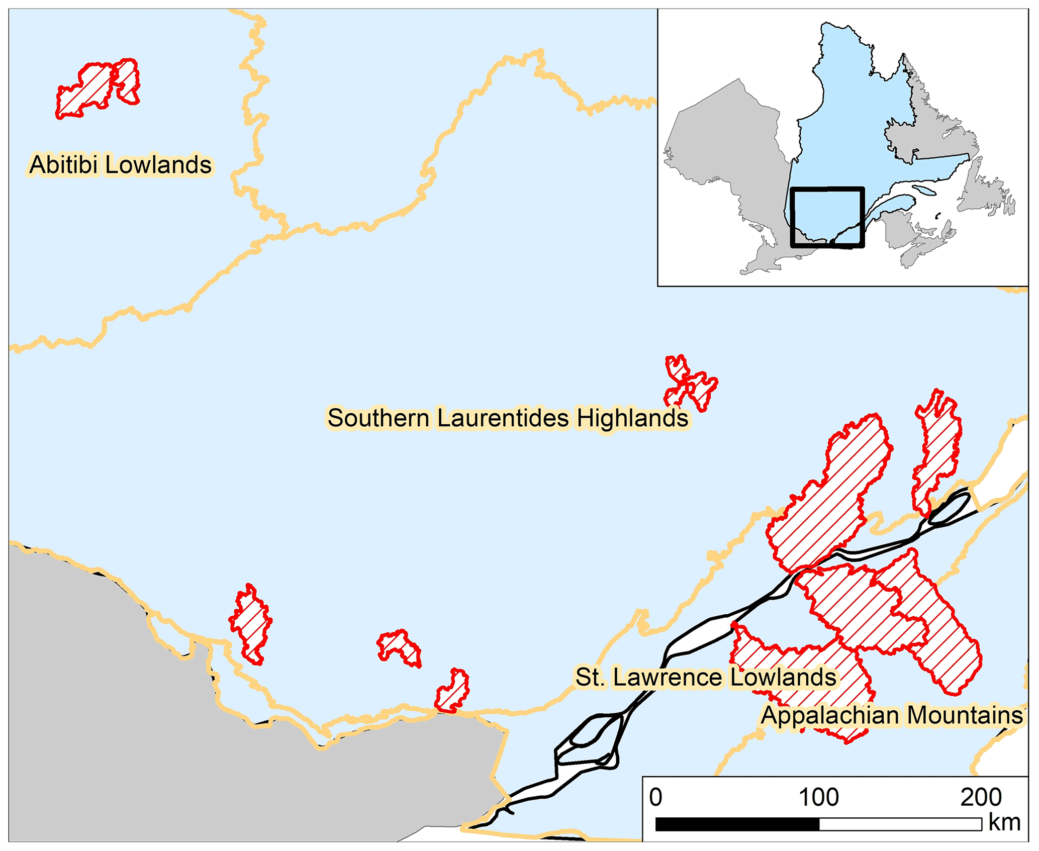
Figure 1 Study areas in the Appalachian Mountains, St. Lawrence Lowlands, Southern Laurentides Highlands, and Abitibi Lowlands natural provinces. Red polygons represent watersheds where field surveys were carried out.

2 Study areas

The study areas were located in the Appalachian Mountains, St Lawrence Lowlands, Southern Laurentides Highlands, and Abitibi Lowlands natural provinces, according to the Quebec Ecological Reference Framework (Fig. 1). This reference framework divides the territory of Quebec into spatially homogeneous units at various, intertwined, levels. The different levels describe homogeneous units in terms of landform, spatial organization, and hydrographic network configuration (Direction de l'expertise en biodiversité, 2018). The diversity of the natural provinces thus selected provides a general representation of the headwater streams in Quebec. These natural provinces have distinct hydrological processes resulting from geological structure and Quaternary deposits.

The Southern Laurentides Highlands is mostly covered by till, the most widespread Quaternary deposit in the province of Quebec (Blouin and Berger, 2004; Gosselin, 2002). This natural province is mountainous, with altitudes varying from 200 to 1200 m. The bedrock mainly consists of gneiss. Quaternary deposits are generally thin on summits and steep slopes and thicker on valley bottoms and gentle slopes. The land in the Southern Laurentides Highlands is largely forested. In the Appalachian Mountains, the Quaternary deposits are somewhat similar in distribution to those in the Southern Laurentides Highlands, although they are thicker in certain areas. However, the bedrock in the Appalachian Mountains is sedimentary and therefore very different from the Southern Laurentides Highlands. The altitude here varies from 0 to 1200 m. Unlike the Southern Laurentides Highlands, there is high anthropization of this natural province due to agriculture (Gosselin, 2005a). In the St Lawrence Lowlands, agricultural activity is also widespread. The Quaternary deposits in this region are highly heterogeneous and are mainly derived from marine and glaciolacustrine geomorphologic processes. These processes lead to thick soils of sorted material, including clay and sand. These, in turn, create deposits that range from impermeable to very permeable. In addition to clay and sand, organic deposits are also present. The elevation of the St Lawrence Lowlands is generally less than 100 m, as it was formed from the Champlain Sea during deglaciation (Gosselin, 2005b). In the Abitibi Lowlands, the Quaternary deposits are rather thick and consist of silt and clay. These deposits were produced by marine and lacustrine invasions and are conducive to the formation of large peatlands. Therefore, the area is relatively flat with altitudes varying from 0 to 350 m. Where present, the bedrock is made of basalt and gneiss (Blouin and Berger, 2002).

Precipitation is not seasonal but rather constant throughout the year in all study areas. Precipitation amounts are quite homogeneous and range from 900 to 1100 mm yr⁻¹, except in the Southern Laurentides Highlands where it can reach 1450 mm yr⁻¹. Approximately 20 % of the precipitation falls as snow during the cold season, except in the coldest regions such as the Abitibi Lowlands and the higher-altitude areas of the Southern Laurentides Highlands where the proportion of snow can reach 30 %. Indeed, the average annual temperature of all the study areas is 3 to 5 °C, except for these two regions where it is 0 °C (MELCC, 2022).

3 Methods

3.1 Field surveys

Field-based data collection is essential to fully understand streamflow patterns. Field surveys were conducted from 2017 to 2021 during summer periods using an EOS GNSS Arrow 100 sub-metre precision GPS. The horizontal accuracy of these devices is ± 0.6 m in open areas and ± 1.2 m in forested areas (Estrada, 2017). These devices were connected to rugged cell phones in order to use the ArcGIS Field Maps application to integrate data collection forms as well as relevant background maps.

The positions of streams were recorded from downstream at drainage areas generally under 1000 ha to upstream until the streambed completely disappeared. The flow regime, the width of the streambed, the extent of the water occupation in the streambed, and the presence or absence of a water flow were collected along the stream path to establish a high level of understanding. A position was taken on the streams every 50 m or so where a streambed was present, i.e. where the stream had a bed floor and banks formed by a fluvial process. Other positions were also taken to identify where there was no streambed. This information was essential for consistent calibration and validation of streambeds.

To ensure consistent data collection, a 50 m × 50 m grid was used to determine which areas should be fully surveyed. These areas were mostly located at headwater streams to be able to include channel heads. This procedure was essential to properly assess the upstream boundary of the headwater streams and precisely record where the streambeds begin, where they flow from the watershed to the perennial stream, and where they are absent.

3.2 Variables used for analysis

The geomatic manipulations were mainly performed with the ArcGIS Desktop 10.7 software package, including the Spatial Analyst and 3D Analysis extensions. The open-source SAGA-GIS (Conrad et al., 2015) and WhiteboxTools (Lindsay, 2016a) software were also used.

The variables used for analysis were produced from 1 m resolution DEMs of the different areas. These were generated from lidar data by the MFFP (Ministère des Forêts, de la Faune et des Parcs), with a density of around 2.5 points m⁻². Lidar acquisitions were conducted from 2016 to 2019 (Leboeuf and Pomerleau, 2015), except for a few areas. The road network was carefully examined to include and burn all culverts that could affect the flow direction (Lessard et al., 2023). Indeed, hydrographic networks are greatly affected by deviations caused by the embankment of the roads. This type of anthropic influence must therefore be minimized to generate a coherent flow direction (Li et al., 2013). Furthermore, the use of a breaching algorithm allowed us to generate hydrologically coherent DEMs prior to hydrographic modelling (Lindsay, 2016b; Lindsay and Dhun, 2015). Physiographic factors must also be considered during the modelling process as they significantly influence the location of channel heads and the flow regime along streams. On the local scale, where the precipitation regime is uniform (Tucker and Slingerland, 1996), slope, hydraulic force, and sediment cohesion generally dictate streambed formation (Dietrich and Dunne, 1978). The influence of these factors is variable depending on the type of Quaternary deposit (Dietrich and Dunne, 1993; Dunne and Black, 1970; Montgomery and Dietrich, 1994).

Quaternary deposits can be used to assess which processes are involved in the formation of a streambed. There are two major types of streambed formation processes. The first type involves surface processes, which occur when soil that has low permeability is exposed to rainfall amounts that exceed the infiltration capacity of the ground, causing surface runoff (Horton, 1945). Then, when the power of the water exceeds the cohesion of the sediments, usually in concavities, a streambed forms (Dietrich and Dunne, 1978). The second type involves subsurface processes that occur when the Quaternary deposits are thick and infiltrative. Water vertically infiltrates into the ground and eventually reaches saturation at a junction with the water table, the bedrock, or an inferior and less infiltrating deposit. Then, lateral movement of the groundwater occurs. Water emerges from the ground when there is a change in slope or soil permeability. Streambeds formed in this way tend to be heavily incised, with flow regimes that are more stable than those formed through surface processes. Thus, the hydrological response of the streams from subsurface processes is slightly affected by the intensity of rainfall (Dunne and Black, 1970; Jensen et al., 2019; Wohl, 2018). Furthermore, it should be noted that there is a gradient between these two processes for each stream. In order to properly detect streambeds, it is essential to distinguish these processes through hydrological classification according to Quaternary deposit type and land use.

Quaternary deposit mapping has been standardized across the province of Quebec and information was collected through photointerpretation conducted several years ago. Since photointerpretation was mainly used to distinguish forest structures and land use, the true boundaries of the Quaternary deposits are imprecise, in some cases. Quaternary deposit boundaries in agricultural areas are more accurate than those in forested areas because no other information was mapped during the process. Regardless of these drawbacks, standardized mapping provides a rough description of the nature and thickness of Quaternary deposits.

Table 1 Hydrological classification according to Quaternary deposit types.

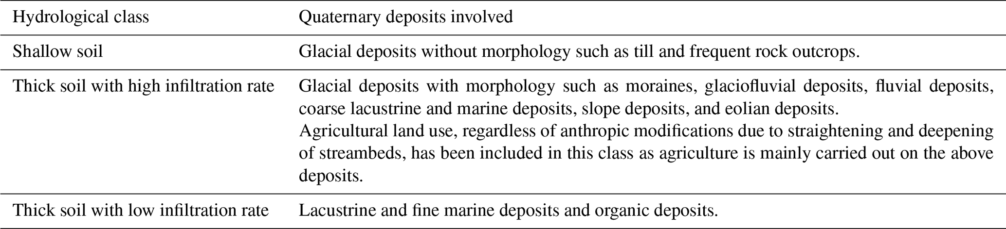
Spatially heterogeneous Quaternary deposits in Quebec have been classified into three categories and are described in Table 1 (Saucier et al., 1994). The purpose of this classification step is to differentiate the two types of hydrological processes for headwater stream formation that were previously described (Dietrich and Dunne, 1993; Lessard, 2020). These classifications consider the infiltration capacity and the water storage capacity of the ground (Dunne and Black, 1970). The two main variables considered were the potential thickness and the granulometry of the Quaternary deposits (Dietrich and Dunne, 1993; Wohl, 2018). Thus, the hydrological classes in Table 1 allow us to group together streams whose formation is driven by similar, and therefore theoretically homogeneous, hydrological processes.

The first analysis variable, called “D8”, refers to the D8 flow accumulation (O'Callaghan and Mark, 1984) produced with a 1 m resolution DEM. This variable was selected as it is the most common algorithm used to produce hydrographic networks. For meaningful correspondence analysis between this variable and field surveyed streams, the flow accumulation raster was aggregated at 3 m resolution according to the maximum value. Then, a maximum focal statistic of two pixels was applied. The purpose of this treatment was to ensure a 6 m analysis distance between the D8 and the edge of a real stream, represented in the database by a vector line feature. This prevents the omission error from being overestimated.

The second analysis variable uses the D8 flow accumulation algorithm while considering flow direction error due to the elevation uncertainty of the lidar-derived DEM (Hengl et al., 2010; O'Callaghan and Mark, 1984). This variable, called “PROB”, quantifies the uncertainty associated with the position of the drainage network. This variable allows water diffusion processes to be simulated more adequately than the multiple flow direction algorithms that have been developed for this purpose (Freeman, 1991). Murphy et al., (2009) noted a convergence of results between the single and multiple flow direction algorithms using high-resolution DEMs derived from lidar data. The use of a multiple direction algorithm did not provide better results for simulating soil moisture. Indeed, the dendritic flow pattern still appeared visible in the wetlands, even with the use of a multiple flow direction algorithm, probably due to the microtopography present in these DEMs. The elevation error in the DEM is directly related to the uncertainty of the lidar data (Wechsler, 2007) and impacts the position of the hydrographic network (Lindsay, 2006). This type of error is affected by the landform and mainly occurs on gentle slopes and slightly convex terrain (Hengl et al., 2010). Since this type of error is inherent to the shape of the land, it is not affected by the size of the drainage area implied. The iterative method described in Hengl et al. (2010) was reproduced in order to create the PROB variable. The method is based on repeatedly computing a flow accumulation raster from an initial DEM and several altered versions of the DEM. These altered versions are created by adding random elevation errors to the initial DEM to reproduce the elevation errors from the lidar data. As described by Richardson and Millard (2018), the typical ground return elevation errors therefore had a standard deviation of 0.08 m, randomly distributed over the DEM. A focal statistic of 3 m was used on the error raster to ensure the spatial autocorrelation of errors. Based on the convergence observed by Lindsay (2006), 50 iterations were carried out. Then, each of the flow accumulation rasters were thresholded to a 1.5 ha drainage area to sum the resulting binary stream network, where a value of 1 indicated the presence of a streambed and a 0 indicated the absence of a streambed. The matrix of the cumulative value was then normalized as a percentage to be used as an analysis variable. This PROB variable revealed the extent of the diffusion process of the water in valley bottoms, small wetlands, or riparian areas, where the slope is relatively low or the topography slightly convex. The PROB variable was produced with a 3 m resolution DEM from a 1 m resolution DEM that was aggregated using the mean values. An average flow accumulation's raster that corresponded to the average of the 50 flow accumulations raster without thresholding was also produced. This raster was used to create the analysis database and to calculate the drainage area of the channel heads. To ensure a 6 m analysis distance as well as the D8 variable, a maximum focal statistic of two cells was performed before summing or averaging the iterated rasters.

The third variable used for analysis is morphometric and allows for the complementary detection of headwater streams (Lindsay, 2006; Tribe, 1992). The morphometric algorithm was the topographic position index, referred to as “TPI”. This algorithm allowed for the local detection of small incisions that might represent streambeds (Tribe, 1992). The scale at which this variable is calculated strongly influences the morphometric feature that is identified. When the scale is large, the variable will tend to identify valleys, while it tends towards streambeds when the scale is small (Montgomery and Dietrich, 1992, 1994). For the purposes of this paper, a relatively small scale of 6 to 30 m was used. This scale is consistent with the width of the majority of inventoried streambeds. The DEM used to calculate this variable had a resolution of 2 m and was derived from aggregating a 1 m resolution DEM with the minimum values. The tool named “Topographic Position Index” in the SAGA-GIS software was used to produce this variable (Guisan et al., 1999; Weiss, 2001). The TPI variable has not been normalized to allow for comparison of the values between the different study areas.

3.3 Analysis database

In order to perform the subsequent analyses, all actual streambeds were vectorized and geo-interpreted according to the stream positions recorded in the field. It should be noted that information on the flow regime was not used in this database. Instead, the presence of a streambed was used to describe the presence or absence of a stream. Although some streambeds have been straightened and deepened, particularly in anthropic lands, streambed was considered to be present only when natural fluvial processes allow it to be maintained. The presence of geo-interpreted vector line features indicated the exact location of the streambeds, and these were complemented by a 50 m × 50 m grid to represent the complete surveyed area. Thus, areas without a vector line feature have been assumed as not containing streambeds.

Positions representing the presence of streambeds were systematically located every 20 m along vector line features that described real streams. Then, positions representing the absence of a streambed were located according to a sampling principle based on minimum flow accumulation where it was still coherent to observe the presence of a streambed. First, within the grid of the surveyed area, the average flow accumulation raster was thresholded at 0.11 ha. This threshold represents the lowest drainage area for initiation of channel head according to Lessard (2020). Then, the resulting raster was converted to a polygon. Following that step, a 20 m buffer zone was removed around the vector line features that represent real streams. Thus, polygons identifying absence positions were located only in areas with a minimum of 0.11 ha mean drainage area and a minimum distance of 20 m from any real streams. Finally, absence positions were systematically located according to a hexagonal distribution in the final resulting polygon. The number of absence positions was equalized with the number of presence positions for each natural region within the Quebec ecological reference framework.

The analysis database was therefore composed of positions describing both the presence and the absence of streambeds (Fig. 2). The values for the three variables described in the previous section (D8, PROB, and TPI) were extracted for all presence and absence positions.

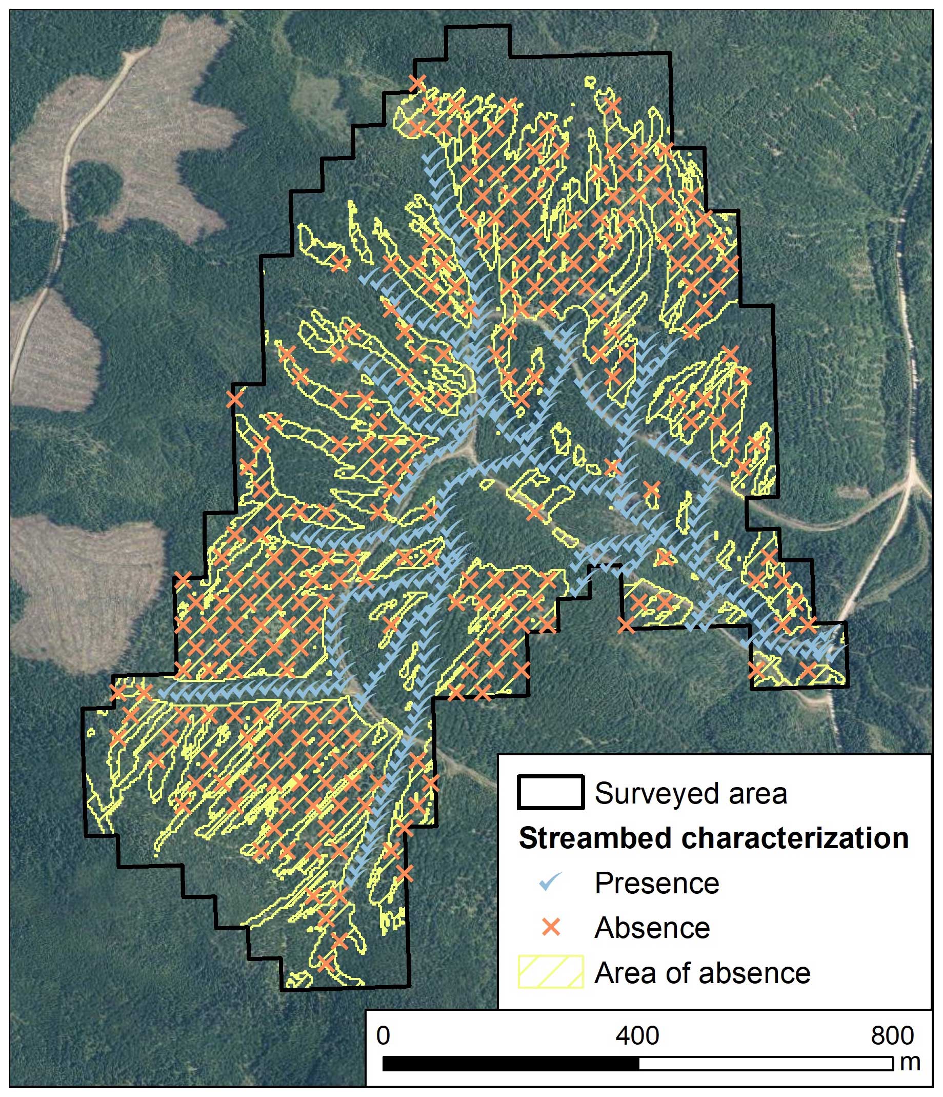
Figure 2 Analysis database of positions indicating the presence and absence of streambeds (Aerial images from continuous imagery of the government of Quebec; MRNF).

3.4 Statistical analysis

A total of nine logistic regression models were produced, one for each explanatory variable and hydrologic class combination. Response variable was the presence (1) or the absence (0) of a streambed. The area under the ROC (receiver operating characteristic) curve was used to evaluate model performance (Fawcett, 2006). The ROC curve plots the true positive rate (1 minus omission) relative to the false positive rate (commission). This curve shows the performance of a given variable by determining the area under the curve (AUC) and how the increase in the true positive rate will lead to an increase in the false positive rate. A model with a high AUC will provide a better balance between these two measurements and will produce better results. Thus, the AUC provides a measure of the ability of the individual variables to detect a streambed.

Next, four streambed models were compared to each other. Detection performance was calculated according to hydrological class and using Cohen's kappa, which is a measure of agreement between the true positive rate and the false positive rate (Cohen, 1960).

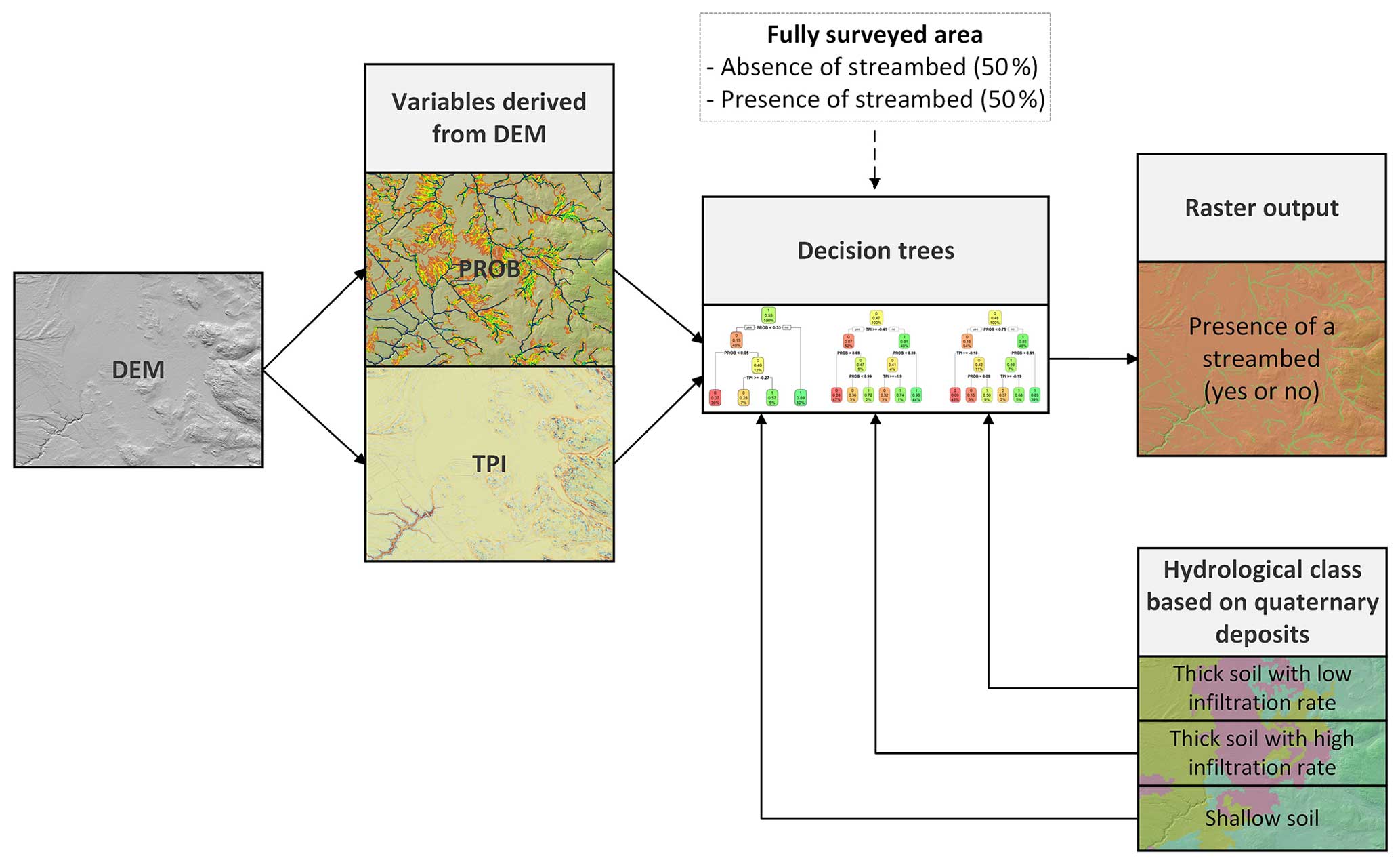
Figure 3 Flowchart showing the methodology used to produce a raster describing the presence of a streambed using classification trees.

The first model examined was the GRHQ. An analysis distance of 6 m was used to compare properly the performance of the GRHQ with the other models. Two of the other three models corresponded to two different thresholds that were applied to the D8 variable, which is one of the most commonly used variables for generating stream networks. The first threshold was the median of the average drainage area of the channel heads surveyed in the field (referred to as “Channel head”; Fig. 3). The second threshold was the one that maximized Cohen's kappa for the variable D8 (referred to as “Max Kappa”). The last model that was compared is based on a supervised classification approach. This approach groups observations according to explanatory variables based on previously determined groups, also known as the response variable. In this case, the response variable was the presence or absence of a streambed. The classification and regression tree (CART) approach was used because of its ease of understanding the results and applying them over a wide area (Breiman et al., 1984). One tree was produced for each hydrologic class in order to describe the formation of headwater streams from homogeneous hydrologic processes.

The TPI and PROB variables were used for each hydrological class to produce trees. A flowchart of the general method is shown in Fig. 3. The depth and number of branches in the classification trees have been pruned in order to prevent overfitting, and it was therefore not necessary to split the data into a training and a testing set (Fürnkranz, 1997).

4 Results

Streams with a total length of 464.7 km were surveyed over an area of 161.5 km². The positions of 1033 channel heads indicating the beginnings of streambeds were determined. The average drainage areas of the channel heads are presented in Fig. 4 using box and whisker plots according to hydrological class. Figure 4 shows that for shallow soil, the average drainage area is less variable than for thick soils. For thick soil with low infiltration rate, the average drainage area tends to be higher. Slope–drainage-area curves and a visualization of different streambeds for each hydrological class are presented in the Supplement.

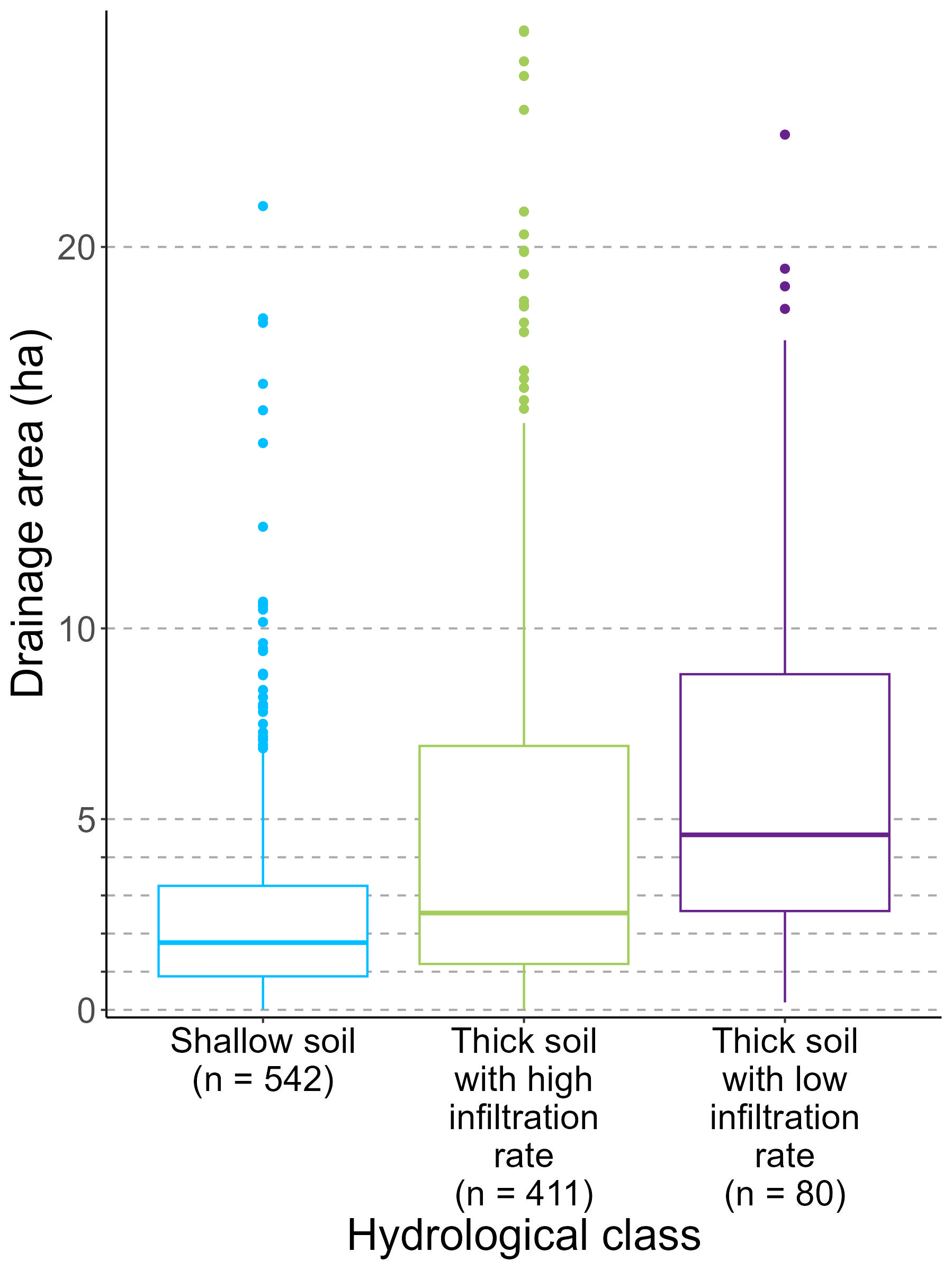
Figure 4 Distribution of mean drainage areas of channel heads according to hydrological class. Median values are shown.

The analysis database contains a total of 40 354 positions describing streambeds (20 177 with streambeds present and 20 177 with streambeds absent). A correlation matrix between the analysis variables showed that PROB is negatively correlated with TPI, with an R of −0.57. This variable therefore identifies where the water converges, which usually corresponds with the locations of incisions. The D8 variable was not correlated with other ones.

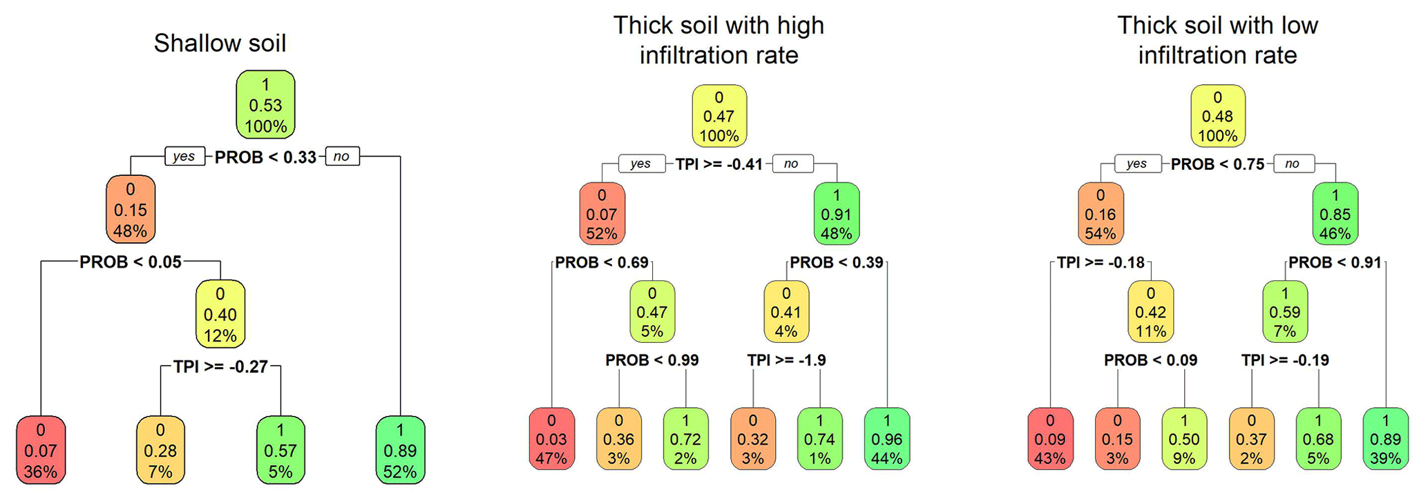
Figure 5 Classification trees to detect the presence of streambeds according to variables D8, PROB, and TPI as well as hydrological class. The colors red, orange, yellow, and green represent very low, low, medium, and high probability, respectively.

The classification trees according to hydrological class are presented in Fig. 5. The tree for shallow soil shows that when PROB exceeds a threshold of 0.33, a streambed is generally present. At the left side of the tree, when the PROB is very low, below 0.05, the streambed is generally absent. Otherwise, the TPI indicates whether a streambed is present or absent. For thick soil with a high infiltration rate, the incision indicated by the TPI first explains the presence of a streambed. When the incision is greater than or equal to −0.41, indicating a small incision, PROB must be very high to indicate the presence of a streambed, at 0.99. When there is a larger incision, a lower value for PROB can identify the presence of a streambed. Thus, when the ground is relatively well incised with a TPI value smaller than −0.41, PROB only needs to be higher than 0.39 to detect a streambed. In thick soil with a low infiltration rate, PROB provides the initial information regarding the presence or absence of a streambed. Depending on the different PROB thresholds, TPI then determines the presence or absence of a streambed.

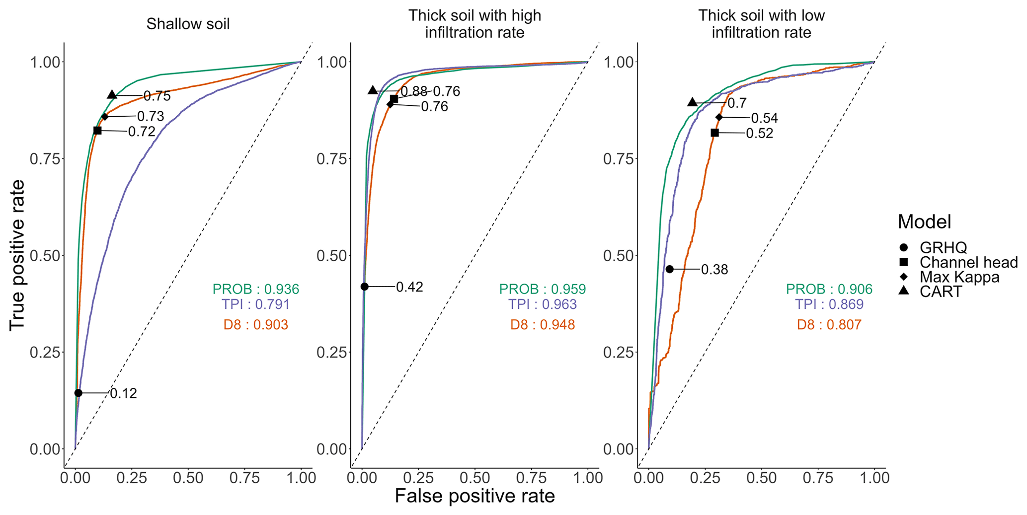
Figure 6 ROC curve and AUC values from the logistic regressions of the three variables according to hydrological class. The performance of the streambed models using Cohen's kappa is also presented.

Figure 6 compares the AUC of individual variables and thus their potential to detect a streambed. The performance of the four streambed models is also presented. This figure shows that for the three hydrological classes, PROB performs more effectively than D8 when it comes to detecting streambeds. For thick soil classes, the incision variable TPI has a higher AUC than D8. For shallow soil, the opposite is true. Compared to the other models, the GRHQ has a very low true positive rate, meaning it omits many streams regardless of the hydrologic class. However, the performance of the GRHQ is higher for thick soil than for shallow soil. For shallow soil, although the false positive rate is slightly lower for D8 thresholded with channel heads (Channel head), the Cohen's kappa of the classification tree (CART) is still higher. The performance of the maximum Kappa of D8 (Max Kappa) is still very similar to the one of the classification tree (CART). Figure 6 also shows that for each class the performance of the classification trees (CART) is in the upper left part of the ROC curve of the variables used alone. This means that the combination of the incision variable TPI with the PROB variable improves the detection of streambeds. For thick soil with high infiltration rate, the two thresholding methods (Channel head and Max Kappa) yielded similar performances, although they did not perform as well as the classification tree (CART). The performance of the classification tree (CART) is also higher than both D8 thresholding methods for thick soil with low infiltration rate. However, the method using the maximum kappa (Max Kappa) yields a higher rate of true positives than the thresholding method using the channel heads (Channel head).

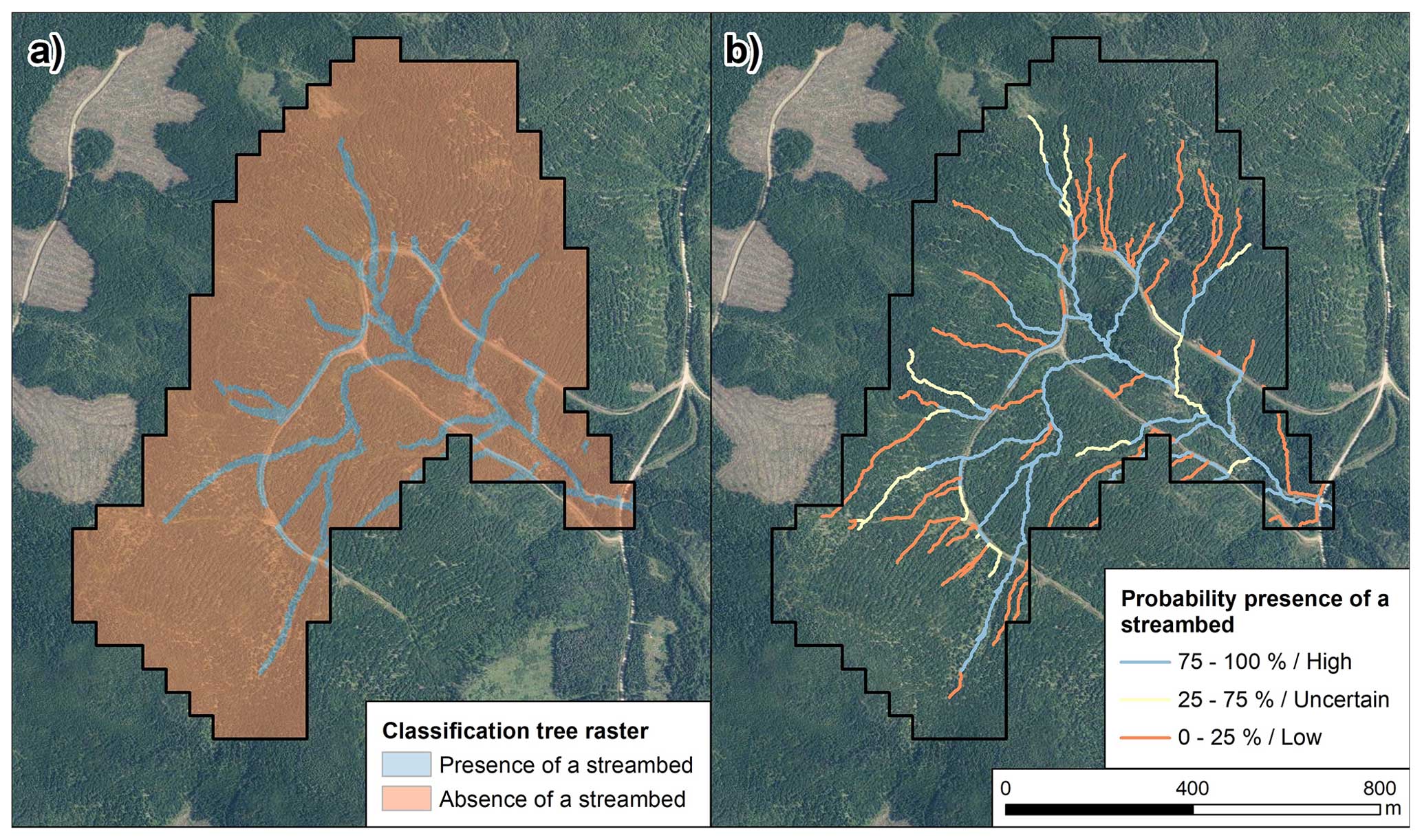
Figure 7 Classification tree that has been integrated into the segments of a hydrographic network to assess the probability presence of a streambed (b) (Aerial images from continuous imagery of the government of Quebec; MRNF).

5 Discussion

The results suggest that the classification tree (CART) can detect streambeds more accurately than the other methods tested. By integrating different topographic indices and ground information such as Quaternary deposits, the detection of headwater streambeds is much more efficient in large watersheds, despite anthropization of the ground as agricultural fields that are sometimes present. In addition, as the results of the classification trees are rasters (Fig. 7a), they can be easily integrated within attribute tables of a drainage network by calculating the mean using a zonal statistic to assess the probability presence of a streambed (Fig. 7b). This integration can be done without altering the course or thresholds of the hydrographic network. Each segment can therefore be truncated according to the presence or absence of the stream predicted by the model.

The classification tree (CART) drastically increases the true positive rate compared to the GRHQ. This is because the GRHQ was based on aerial photographs that were primarily used to characterize vegetation and forest structure. Photointerpretation of these images did not allow for the detection of streambeds formed by local fluvial processes under the forest cover (Lessard, 2020). At most, photointerpretation enables the identification of valleys, for example, on thick soil (Montgomery and Dietrich, 1994). For this reason, the GRHQ omits fewer streams in thick soil than in shallow soil.

The PROB variable improved the detection of streambeds compared to the conventional use of only the D8 variable, since it has been thresholded to accurately match the lowest drainage areas of the channel heads. According to Fig. 4, the 1.5 ha threshold accounts for most of the channel heads. However, the drainage areas of the channel heads are generally higher for thick soil with low infiltration rate and could therefore lead to a higher false positive rate. Most of the surveyed streams in this hydrologic class are located in the Abitibi Lowlands natural province. Furthermore, it is important to note that some of the drainage areas of the channel heads in shallow soil are smaller than 1.5 ha.

For the shallow soil hydrological class, the PROB variable improves streambed detection only when a false positive rate of at least 0.12 is specified. Figure 6 shows that for a false positive rate of 0.25, for example, PROB has a higher true positive rate than the D8 variable. Streambeds that were not omitted with a PROB threshold greater than 0.12 were mostly small streams with highly variable positions due to the slightly upstream convex topography (Hengl et al., 2010). It seems that these streambed presence positions have very low PROB values (48 % of these positions have a probability below the 0.33 threshold used; Fig. 5). The 0.33 PROB threshold enabled a false positive rate that is much lower than 0.25. In fact, the false positive rate was only 0.12. With this 0.33 threshold, the performance of PROB was almost identical to D8 (Fig. 6). To increase the true positive rate while using the PROB variable, the threshold could be decreased to allow the smallest streams to be identified. However, this modification would increase the false positive rate.

The poor performance of the TPI variable for shallow soil is due to the fact that the Quaternary deposits are generally thin and the slopes are frequently steep. The ground is therefore less prone to erosion and incision than for the other two hydrological classes (Jensen et al., 2018; Montgomery and Dietrich, 1994). Indeed, the parameters used to compute TPI do not enable the detection of small streambeds if they are not located in a valley or in a larger incision. Furthermore, the hydrological processes involved in this class are mostly surface flow and not subsurface flow. It is for this reason that D8 and PROB, which tend to be able to recreate surface flow quite precisely, are the best performing variables in this hydrological class (Julian et al., 2012; Wohl, 2018).

The incision variable TPI performed better in thick soil with high infiltration rate. This seems to be due to the fact that unlike shallow soil which are generally thin, infiltrative soil are thick and unconsolidated. Thus, the main hydrological process for this hydrological class is a subsurface process, where the water table plays an important role in the initiation of streambeds. Water infiltrates vertically into the permeable deposits and recharges the groundwater (Dunne and Black, 1970). The locations of the channel heads do not correspond to specific drainage areas that can be identified by flow accumulation variables but rather to local incisions formed by gullying processes where groundwater intersects the ground surface (Dietrich and Dunne, 1993; Wohl, 2018). This process occurs where there is a significant change in slope or soil permeability. The emergence of water from the ground leads to progressive gullying that can be detected by incision variables (Montgomery and Dietrich, 1994). In this context, groundwater depth variables such as depth-to-water (DTW; White et al., 2012) could be used to explain the presence of streams in areas where a water table is present. It is important to mention that the DTW is very sensitive to parameterization, and more research is needed for its proper use (Drolet, 2020).

Streambeds were better detected using solely PROB instead of D8 for thick soil with low infiltration rate, which occur in territories where there is a high proportion of wetlands and gentle slopes. The PROB variable mostly reduces the number of commission cases. For example, in Fig. 6, PROB had a much lower false positive rate than D8 for the same true positive rate of 0.75. This large reduction in the false positive rate achieved with PROB reflects the ability of this variable to reproduce a diffuse flow on very flat or slightly convex terrains (Hengl et al., 2010). Indeed, in 78 % of cases, the positions that correspond to an absence of a streambed and that are corrected with PROB are wetlands. This is noteworthy, because wetlands represent only 64 % of these positions in this hydrological class. Thus, the PROB variable, using uncertain DEM elevation information, can recreate more realistic behaviour of the water, especially in thick soil with low infiltration rate. By using both PROB and TPI variables (Fig. 5), streambed detection for this hydrological class can be improved compared to the use of a single variable. Because the deposits are unconsolidated and the ground can be incised (Dietrich and Dunne, 1993), the classification tree is in the upper left part of the ROC curve for the PROB variable as well as for the hydrological class with the high infiltration. The use of the TPI variable therefore provides an advantage.

A limitation of the classification tree method is that the Quaternary deposit mapping is not accurate enough for all local hydrological issues. A visual inspection revealed some inconsistencies in the Quaternary deposit mapping within the same hydrological class.

Another limitation is associated with the anthropization and straightening of natural streams. While a streambed is the result of a natural fluvial formation process that leads to ground erosion, an anthropic ditch is an artificial bed that is formed by mechanized digging. However, it is common for naturally formed streambeds to have been excavated and straightened in agricultural areas. In these cases, it becomes very difficult to distinguish a streambed from an anthropic ditch, even in the field. Excavation concentrates the flow of water in the artificial bed (Moussa et al., 2002). Thus, an area with previously no water flow could now be considered a streambed (Roelens et al., 2018). Automated detection methods are therefore likely to be much less reliable in these situations.

We believe that the method described for calibrating the classification tree model is simple and robust enough to be applied in a different climatic and geomorphologic context with local data describing headwater streambeds. An accurate lidar-derived headwater streambed mapping is a powerful tool for government and local organizations involved in water management and protection.

6 Conclusion

The classification tree method presented in this paper has improved the detection of headwater streambeds for different hydrological processes over large watersheds. Reliable and consistent results were obtained by developing a comprehensive field database. The variable PROB, which describes the probability of occurrence of a streambed, was used to correct errors associated with the positioning of streambeds. This variable allowed for marginal corrections of streambeds in shallow soil, particularly when a high threshold was used. In order to more precisely explain where streams initiate in shallow soil, variables characterizing the composition of the upstream watershed such as the average upstream slope or the composition of deposits should be explored. The variable TPI, which characterized small-scale incisions, significantly improved the detection of streambeds in both thick soil hydrological classes when combined with the PROB variable. The small-scale incision variable worked better in soil with high infiltration rate, and the probability of occurrence worked better in soil with low infiltration rate.

The increased complexity of the methods (inputs and parameterization) makes the optimizations more difficult for large and complex territories. The integration of all physiographic variables into a single model requires multiple iterations which leads to high complexity. Case studies could improve models by directly focusing on some of the identified limitations. It is also important to consider that the input data may sometimes be unreliable, such as those for the road network, culverts, Quaternary deposits, and land use. Thus, future developments, such as those integrating Quaternary deposits, will hardly be possible if the quality of the raw data remains unchanged. Visual interpretation of map products and verification by an expert with a good knowledge of the area is an essential step that should not be neglected under any circumstances.