Influence of vegetation maintenance on flow and mixing: case study comparing fully cut with high-coverage conditions

In temperate climates, agricultural ditches are generally bounded by seasonal vegetation, which affects the hydrodynamics and mixing processes within the channel and acts as a buffer strip to reduce a load of pollutants coming from the surrounding cultivated fields. However, even if the control of such vegetation represents a key strategy to support sediment and nutrient management, the studies that investigated the effect of different vegetation maintenance scenarios or vegetation coverage on the flow and mixing dynamics at the reach scale are very limited. To overcome these limitations and provide additional insights into the involved processes, tracer tests were conducted in an agricultural ditch roughly 500 m long close to Warsaw in Poland, focusing on two different vegetation scenarios: highly vegetated and fully cut. Under the highly vegetated scenario, sub-reaches differing in surficial vegetation coverage are analysed separately to better understand the influence of the vegetation conditions on the flow and mixing parameters. Special attention has been paid to the longitudinal dispersion coefficient in complex natural conditions and its dependency on vegetation coverage (V). The vegetation maintenance decreased the travel and residence times of the solute by 3–5 times, moderately increasing the peak concentrations. We found that the dispersion coefficient decreased approximately linearly with the increase of vegetation coverage at V>68 %. Further research is needed at lower vegetation coverage values and different spatial plant distributions. The obtained longitudinal dispersion coefficient values complement dispersion value datasets previously published in the literature, which are barely available for small natural streams. The new process understanding supports the design of future investigations with more environmentally sound vegetation maintenance scenarios.

1 Introduction

Despite the crucial role of aquatic and riparian vegetation in keeping riverine ecosystems healthy (Rowiński et al., 2018; Soana et al., 2019), extensive vegetation cutting is widely practised to enhance the flow conveyance, e.g. for flood and agricultural water management. While environmentally friendlier vegetation maintenance practices and channel designs have been proposed in the past (Buisson, 2008; SEPA, 2009), traditional ecologically harmful cutting and dredging practices continue to be applied, despite their large-scale negative influences on agricultural streams and rivers (Old et al., 2014; Bączyk et al., 2018). In two-stage channels and other nature-based designs, clever, environmentally friendlier vegetation maintenance may provide possibilities for enhancing the retention of suspended sediment and nutrients while maintaining flow conveyance (e.g. Kindervater and Steinman, 2019; Västilä et al., 2021). However, optimising the performance of such vegetated channel designs requires an improved understanding of the influence of spatially variable vegetation distributions on transport and mixing processes (Rowiński et al., 2022).

In most cases, plants do not cover the entire channel cross-section but grow preferably along the banks, while the deepest parts of the channel remain bare. In such partly vegetated channels, aquatic macrophytes are often arranged in patches or strips, and this arrangement can be influenced, among many other factors, by very local management practices (Old et al., 2014). In this respect, a growing number of studies demonstrated that the influence of vegetation on the flow hydraulics significantly depends on the plant arrangement, such as patch shape, density, and coverage (e.g. Helmiö, 2002; Pan et al., 2019; Yang et al., 2019; Cornacchia et al., 2020). Despite field investigations on the hydraulic influence of vegetation cutting (e.g. Verschoren et al., 2017; Baattrup-Pedersen et al., 2018; Errico et al., 2019), field-based quantitative relationships between the extent of vegetation cutting and its influence on the flow hydraulics are still limited. From a more holistic viewpoint, research gaps remain regarding the overall efficacy of vegetation maintenance practices and their influence on species distribution in lowland channel networks (Errico et al., 2019). Choosing the most appropriate vegetation maintenance practice along ditches is a key issue in agricultural water management (Forzieri et al., 2012).

To support river management, it is critical to find straightforward but physically sound parameters to describe the impact of vegetation. For partly vegetated channels colonised by herbaceous plants, the key factor determining the flow resistance and flow hydrodynamics is the vegetative blockage, i.e. the ratio between the area covered by vegetation and the total wetted area (e.g. Luhar and Nepf, 2013; Kiczko et al., 2020; Rudi et al., 2020). To capture the transition between submerged and emergent vegetation, the vegetative blockage can be considered as the cross-sectional blockage (Västilä and Järvelä, 2018). As such detailed parameters may be infeasible to measure under some field conditions (e.g. Perret et al., 2021), for agricultural channels with low water depths and mostly emergent vegetation, the vegetative blockage can be considered as the planform blockage, i.e. surficial coverage, which can be obtained from aerial images and remotely sensed information. Given their high precision and relatively low deployment costs, uncrewed aerial vehicles (UAVs) are frequently used in agricultural areas nowadays (e.g. Gago et al., 2015; Mogili and Deepak, 2018; Masina et al., 2020) in addition to satellite information (Bretreger et al., 2020).

Although the influence of vegetation distribution on the flow and mixing has recently received growing attention, the understanding of how vegetation maintenance affects the mixing and transient storage of both solutes and particles is still rather limited (Verschoren et al., 2017; Kalinowska et al., 2019; Västilä et al., 2022). Firstly, most works on mixing in vegetated flows are limited to selected, very specific vegetation setups, mostly in laboratory conditions, usually focused on fully vegetated conditions with vegetation growing on the entire channel bed. Secondly, it should be kept in mind that the rate of mass transport cannot be directly estimated based on the rate of momentum transport in vegetated flows (Ghisalberti and Nepf, 2005). Thirdly, the applicability of the traditional scaling of the so-called longitudinal dispersion (D_L) coefficient describing the rate of spreading (dispersion) of the solute in the streamwise direction by the shear velocity to vegetated flows is debatable (Shucksmith et al., 2010).

The longitudinal dispersion coefficient is present in the 1D advection–diffusion/dispersion equation (ADE), commonly used to describe the mixing and transport of admixture in open channels, as a result of averaging the 3D ADE over the channel depth and width. The values of the longitudinal dispersion coefficient are required to run numerical models to simulate the spread of pollutants in time and space. Dispersion coefficients are in fact the most important and, at the same time, the most difficult to determine factors characterising the mixing processes (Czernuszenko, 1990; Kalinowska and Rowiński, 2012). It is still challenging to determine their values for a particular channel (Kalinowska and Rowiński, 2012), especially for natural channels with vegetation.

Recent laboratory work with rigid cylinders used to mimic vegetation (Park and Hwang, 2019) indicates that the dependency of longitudinal dispersion on the vegetation arrangement is highly complex and controlled by the total clumpiness of the vegetation in the longitudinal and lateral directions across the channel reach. To support devising suspended matter and nutrient management strategies, further real-scale studies are needed on the influence of vegetation maintenance focusing on the longitudinal dispersion, the residence time distributions, and the peak concentration in small natural channels, where vegetation is clearly the main factor controlling the flow (Västilä et al., 2016).

Using an agricultural ditch in Poland as a case study, this work aims to improve understanding of the influence of vegetation management practices on flow hydraulics and mixing. Our primary focus is the determination of the longitudinal dispersion coefficients and their dependence on the vegetation coverage. Tracer experiments remain the best source of information for estimating their values under complex, natural conditions. Our tracer tests focus on the two most common maintenance scenarios: no maintenance (fully vegetation) and complete vegetation cut (bare channel). The experiments were conducted at low-flow conditions, and it is beyond the scope of the paper to analyse a range of hydraulic boundary conditions.

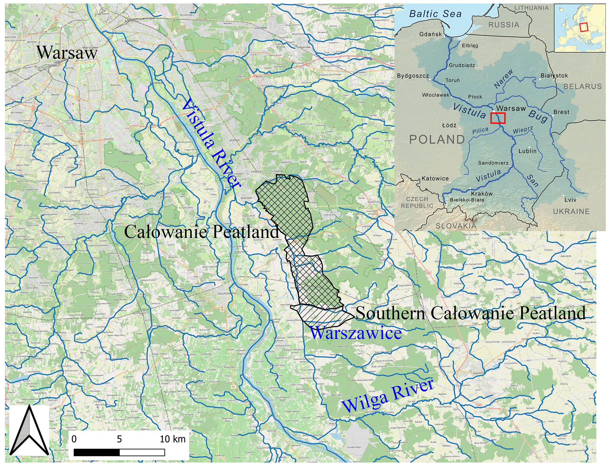
Figure 1 Location of the Całowanie Peatland Protected Area, south of Warsaw, Poland. The Warszawicki Channel is located close to the boundaries of the Southern Całowanie Peatland. © OpenStreetMap contributors  021. Distributed under the Open Data Commons Open Database License (ODbL) v1.0. Small top, right map of Poland, adapted from Nones (2021).

2 Materials and methods

2.1 Study site

The Warszawicki Channel is located close to the boundaries of the largest peat bog in Mazovia – Bagno Całowanie (Całowanie Peatland, covering 35 000ha), located in the Mazowiecki Landscape Park, about 40 km south-east of Warsaw, Poland, in the Vistula River valley (Fig. 1). In the past, large parts of peatland were reclaimed for agricultural purposes, and the Warszawicki Channel served as a water source for irrigation. The total catchment area is around 240 km² and, in a hydrographic sense, it links the Wilga River system with the Vistula River to divert surface water reserves to the area of the Całowanie Peatland. The channel is also connected with several smaller watercourses to provide sufficient flood protection to the areas located between the Wilga and Vistula rivers. Indeed, those channels were designed to retain part of the floodwaters of the Vistula River to mitigate excess water hazards.

The experiments were conducted in a reach, about 500 m long, of the Warszawicki Channel. This channel was selected due to the varying cross-sectional vegetation patterns resulting from natural vegetation growth (see Fig. 2). Typically, mechanical cutting and removal of bank and bottom vegetation are planned twice a year, with the local legislation requiring maintenance at least once per year. This fact might create variable conditions for the water flow or the solute transport, mostly due to different stages of plant development in the channel bed. In 2019, the channel vegetation was cleared only once at the beginning of October, using an excavator with a weed cutting bucket, and the channel bed was not dredged. These conditions were favourable for the present study, given that at the end of the summer, the channel vegetation was very dense, as shown in Fig. 3a.

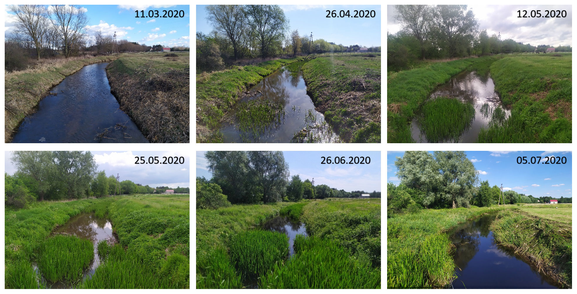
Figure 2 Selected photos of the vegetation photo monitoring conducted in the Warszawicki Channel during 2020. Pictures show the situation from the winter conditions – before vegetation started to grow (left top image) until the channel maintenance cleaning in summer (right bottom photo). The monitoring was carried out as part of the BRITEC citizen science project (https://britec.igf.edu.pl/, last access: 28 February 2023). Photos taken by pupils from the primary school in Warszawice.

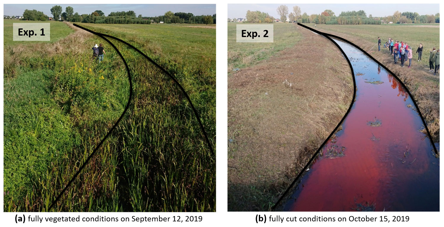
Figure 3 Warszawicki Channel – view towards the downstream sub-reaches (a) before and (b) after the vegetation cutting.

We selected four sub-reaches (A between cross-sections P1 and P2, B between P2 and P3, C between P3 and P4, and D between P4 and P5) with varying vegetation coverage (see Fig. 4 for details). Their lengths differed as we attempted to delineate the sub-reaches so that a large range in the vegetation coverage could be obtained. We conducted investigations during fully vegetated conditions (Exp. 1, no maintenance, September 2019) and after complete cutting and removal of the channel and bank vegetation (Exp. 2, fully cut, October 2019). Figure 3 presents the channel view towards the downstream sub-reaches before (Fig. 3a) and after (Fig. 3b) the vegetation cutting.

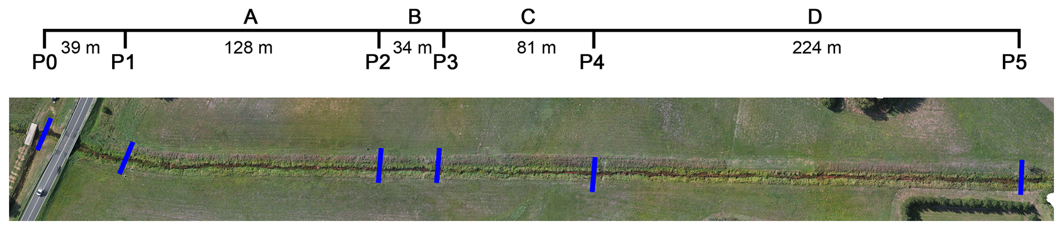
Figure 4 Aerial image captured in fully vegetated (Exp. 1) conditions and a scheme with marked cross-sections of the analysed reach of the Warszawicki Channel.

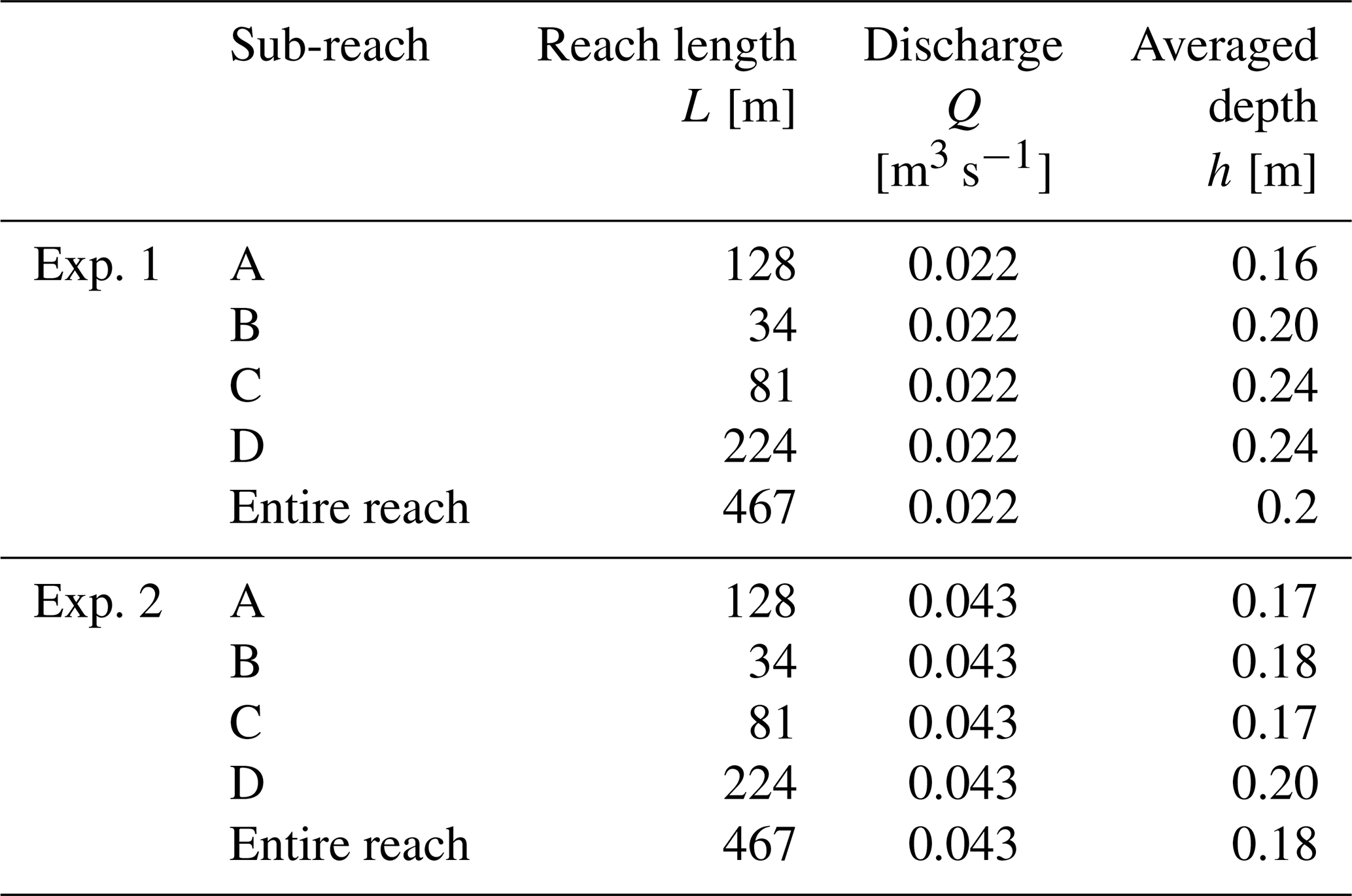
Table 1 summarises the main properties of the four selected channel sub-reaches and the entire 467 m long reach, located between the P1 and P5 cross-sections (sub-reach ABCD), during both experiments. The flow discharge (Q) was roughly estimated based on flow velocity measurements performed before each tracer experiment in a few selected, well-accessible, cross-sections with reduced vegetation coverage. Flow velocity distributions were measured using an electromagnetic flow meter (Nautilus C 2000 OTT) to derive the flow discharge by integrating the point velocity measurements across the wetted cross-sectional area. There is increased uncertainty in the calculated flow rates due to lower water levels and the presence of vegetation in the channel affecting cross-sectional velocity measurements. No extreme events (e.g. heavy rainfalls and droughts) were recorded in the study period between the two experiments. However, during the field campaigns, controlling all environmental factors influencing the hydraulic conditions was not feasible, and possibly increasing uncertainties in the final estimations of the flow discharges should be considered. The channel slope was around 0.1 ‰. The slope was measured by multiple geodetic levelling of the water surface over 60–100 m. As is visible in Table 1, both experiments were performed with a comparable reach-averaged water depth. However, the water depth was slightly lower, particularly in the two most downstream sub-reaches in Exp. 2.

Table 1 Main properties of the four sub-reaches and the entire analysed reach of the channel during the experiments with (Exp. 1) and without (Exp. 2) vegetation.

2.2 Surficial vegetation coverage

Unlike most available studies, the research proposed in the paper is not focused on individual plants or patches but on vegetation coverage at the reach scale in complex natural conditions.

Species that may be present in the Warszawicki Channel include the following: Phalaris arundinacea L., Phragmites australis, Glyceria maxima and Sparganium emerson, forming mixed, mostly emergent vegetation (Fig. 5). Contrary to laboratory investigations where researchers can deal with controlled and well-described hydraulic and vegetation properties, in the field we are dealing with mixed vegetation (e.g. submerged and emerged, different species and densities). During our experiments, we did not collect detailed physical information on the particular plants growing in the channel. Instead, we aimed to investigate the influence of vegetation at the reach scale, and it is known that at the reach scale, the coverage is the factor mainly influencing the flow hydraulics (Green, 2005; Luhar and Nepf, 2013). Thus, we hypothesised that the solute transport would also depend on coverage. Practical applications with “disorderly” natural vegetation motivated our work to investigate physically sound but easily measurable parameters like vegetation coverage.

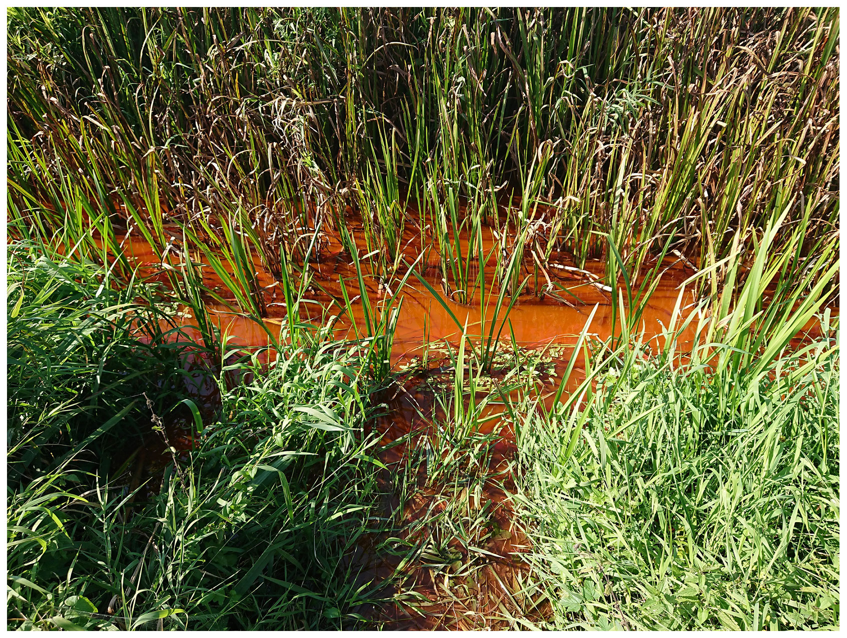
Figure 5 Sample photo showing complex vegetation in the Warszawicki Channel, taken during Exp 1.

The surficial vegetation coverage (V) of the studied reach was determined through UAV imagery using a DJI Phantom 4 drone equipped with an RGB camera (Fig. 6). To ensure comparability of measurements during the experiments, the drone flights were performed in automatic mode with the same flight parameters and camera settings and similar weather conditions. In addition, the Pix4D application was utilised for programming and automatic implementation of the fully photogrammetric UAV missions. The flight took place at a speed of 4 m s⁻¹ at a height of 35 m above ground with 70 % image overlap. The resolution of the obtained data was 1.5 cm. Three flight missions were carried out in a time interval of 40 min for the fully vegetated scenario and 10  min for the fully cut scenario, conditioned by the different velocities of the plume movement.

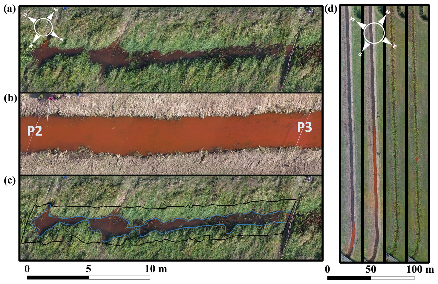
Figure 6 Aerial image of the sub-reach B, captured in (a) fully vegetated (Exp. 1) and (b) fully cut (Exp. 2) conditions. (c) The surface coverage of vegetation was determined by computing the ratio of the vegetation-covered surface area and the total wetted surface area available from the bare-channel scenario. (d) Example orthophotos of the entire analysed reach taken during the tracing, with the two leftmost photos showing the cut condition and the two rightmost photos showing the vegetated condition.

Based on the collected images, orthophoto maps were generated using the Agisoft PhotoScan software, applying the Structure-from-Motion (SfM) method (Mlambo et al., 2017; Carrivick and Smith, 2019). Those maps were analysed in the open source Quantum Geographic Information System (QGIS) (https://www.qgis.org, last access: 28 February 2023) to determine the surficial vegetation coverage in the channel in the case of fully vegetated conditions (light blue line in Fig. 6c, Exp. 1) as well as the precise location of the river bank line for the bare conditions (black line in Fig. 6c, Exp. 2). Similar water levels in the river channel during the two experiments (see Table 1 in Sect. 3) allowed the assumption that the bank line determined at the cut conditions was representative of the fully vegetated conditions.

Using map algebra, widely used in GIS studies (Câmara et al., 2005), the percentages of vegetation coverage for the entire examined reach (between P1–P5 cross-sections) and for each individual sub-reach (see Fig. 4) were calculated according to Eq. (1):

$$\begin{array}{}\text{(1)}& V={\displaystyle \frac{W_{\mathrm{C}}-W_{\mathrm{V}}}{W_{\mathrm{C}}}},\end{array}$$

where V is the surficial vegetation coverage, W_C is the surficial water area in the channel under bare conditions (polygon marked with a black line in Fig. 6c), and W_V is the surficial water area in fully vegetated conditions (polygon marked with a blue line in Fig. 6c). In the case of Exp. 2 (fully cut conditions), V was assumed to be 0 %.

2.3 Tracer tests

For the tracer experiments, we used Rhodamine WT which is a soluble, non-toxic fluorescent dye, conservative at the considered timescales (Smart and Laidlaw, 1977; Rowiński et al., 2008; Rowiński and Chrzanowski, 2011). It is detectable in very low concentrations, and it has been used over many years in laboratory and field studies to estimate travel times, mean flow velocities, or dispersion coefficients in streams and rivers (e.g. Kilpatrick and Wilson, 1989; Wallis et al., 1989; Boxall et al., 2003; Rowiński et al., 2008; Socolofsky and Jirka, 2005; Julínek and Říha, 2017). In both Exp. 1 and Exp. 2, the Rhodamine WT was released instantaneously at P0, a non-vegetated area located 39 m upstream of P1 (see Fig. 4). The dye concentration was measured at the cross-sections P1, P2, P3, P4, and P5 downstream of the injection point over a total distance of about 500 m. Distances between the sampling locations were 128, 34, 81, and 224 m for sub-reach A, B, C, and D, respectively (see Fig. 4).

The water samples were manually collected from the central part of each cross-section using an aluminium sampling rod with the personnel standing outside the water without disturbing the flow. The samples were stored in black bottles to prevent rhodamine loss due to exposure to light. They were analysed in the laboratory under controlled temperature conditions with a 10-AU-005-CE fluorometer from Turner Designs. Furthermore, for Exp. 2, a handheld fluorometer (Turner Designs, AquaFluor handheld fluorometer) was used to check the concentration values in real time since the passage of the plume was very fast. This information was used to adjust the sampling frequency to ensure that the leading edge of the dye cloud and the concentration peak were captured correctly. We changed the sampling frequency based on expected/checked concentration values to optimise the usage of bottles for samples and the laboratory's sample measuring process.

During Exp. 1, we started sampling with 10 min intervals (except for the cross-section P1, when we started immediately with 5 min intervals). Then, the sampling frequency was increased to 5 min close to the expected peak (2–3 min for P1) and returned to 10 min (after the peak was captured). Finally, we measured from 10 to 60 min for the tailing edge as the concentration changed more and more slowly. In the case of non-vegetated conditions (Exp. 2), since the passage of the dye plume was quick, we sampled faster. Sampling frequency varied from 1 to 10 min. We sampled more frequently, close to the expected peak of concentration (from 30 s in P1 to 1–3 min in other cross-sections), and less frequently for the tailing edge from 5 to 10 min. The sampling period was adjusted to the actual cross-section concentration changing (using a handheld fluorometer on site).

Before starting both experiments, a few water samples were taken to establish the background concentration. Additional samples were taken during the experiments upstream of P0 to check that the background concentration was not changing. Background water samples have also been used for calibration and appropriate timing of the end of the sampling. For accuracy checking, Exp. 2 was repeated later on the same day under the same hydrological conditions after reaching the background values of the concentration (Exp. 2'). For Exp. 2', water samples were collected at selected cross-sections (P1, P2 and P4).

2.4 Data analysis

We derived parameters describing flow and mixing based on the obtained parameters during tracer test concentration data. They were derived separately for each sub-reach and the entire reach (P1–P5) based on the concentration curves at the corresponding upstream and downstream cross-sections (see Sect. 2.3).

The peak travel time (t_p) and peak concentration (C_max) were derived directly from the concentration distributions for each measured cross-section. Different methods may be applied to obtain the flow velocities and dispersion coefficients. The most commonly used are the method of moments and the routing procedure, described and compared, e.g. by Heron (2015). The second one required fixed time intervals in the concentration distribution. Taking into account our sampling procedure, we applied the method of moments (Rutherford, 1994), well-established and used for many years in tracer studies (for details see e.g. Kilpatrick and Wilson, 1989; Wallis et al., 1989; Boxall et al., 2003; Socolofsky and Jirka, 2005; Heron, 2015; Julínek and Říha, 2017). This method was initially proposed by Fischer (1966), and nowadays, it is widely used in field and laboratory tracer studies, mainly for determining the longitudinal dispersion coefficient (D_L).

The longitudinal dispersion coefficient value was determined based on the changes in the centroid and variance of the recorded temporal concentration distributions between two cross-sections. For each sub-reach j located between two sampling cross-sections (“1” – upstream and “2” – downstream cross-section), $D_{\mathrm{L}}^j$ was obtained from

$$\begin{array}{}\text{(2)}& D_{\mathrm{L}}^j={\displaystyle \frac{U_j^{\mathrm{2}}\left({\mathit{\sigma }}_t^{\mathrm{2}}\left(x_{\mathrm{2}}\right)-{\mathit{\sigma }}_t^{\mathrm{2}}\left(x_{\mathrm{1}}\right)\right)}{t_{\mathrm{c}}^{\mathrm{2}}-t_{\mathrm{c}}^{\mathrm{1}}}},\end{array}$$

where x_i is the location of the ith cross-section, $t_{\mathrm{c}}^i$ represents the time of passage of the centroid of the dye plume in ith cross-section, U_j indicates the mean velocity of the plume in the sub-reach j and ${\mathit{\sigma }}_t^{\mathrm{2}}\left(x_i\right)$ is the variance of temporal concentration distribution in the ith cross-section. The sub-reach mean velocity U_j is computed as

$$\begin{array}{}\text{(3)}& U_j={\displaystyle \frac{x_{\mathrm{2}}-x_{\mathrm{1}}}{t_{\mathrm{c}}^{\mathrm{2}}-t_{\mathrm{c}}^{\mathrm{1}}}}.\end{array}$$

Based on the values of centroid travel times obtained at the upstream $t_{\mathrm{c}}^{\mathrm{2}}$ and downstream $t_{\mathrm{c}}^{\mathrm{1}}$ cross-sections of each sub-reach, the mean sub-reach centroid travel time was calculated as

$$\begin{array}{}\text{(4)}& T_{\mathrm{c}}=t_{\mathrm{c}}^{\mathrm{2}}-t_{\mathrm{c}}^{\mathrm{1}}.\end{array}$$

The weakness of the method of moments is that the distribution variance is sensitive to concentration fluctuations in the tails of the concentration distributions. To increase the accuracy, the concentration distributions were cut at the point when concentration dropped below 0.5 % of the maximum concentration in the given cross-section, following the experience and recommendation of other scholars (e.g. Yotsukura et al., 1970; Heron, 2015).

The influence of the vegetation cut on the mean velocity were characterised as $U_{\mathrm{NV}}/U_{\mathrm{VEG}}$, where the subscript NV refers to the non-vegetated and VEG to the vegetated conditions, respectively.

3 Results and discussion

Normalised temporal concentration distributions for all sampled cross-sections (P1–P5) are presented in Fig. 7a) for vegetated (Exp. 1) conditions and in Fig. 7b) for non-vegetated (Exp. 2) conditions. The concentrations have been normalised by the maximum concentration value recorded in the first cross-section P1. Data are also available in a dataset (Kalinowska, 2022). The presence of vegetation, causing low velocities, resulted in reaching the peak concentration at the first sampling cross-section P1 around 12 min from the tracer release, while concentrations decreased to the background in less than 3 h. By contrast, the passage of the plume was notably faster after the vegetation cut (Fig. 7b), with the peak concentration reached around 3 min from the release at P1 and concentrations decreased to the background in less than half an hour.

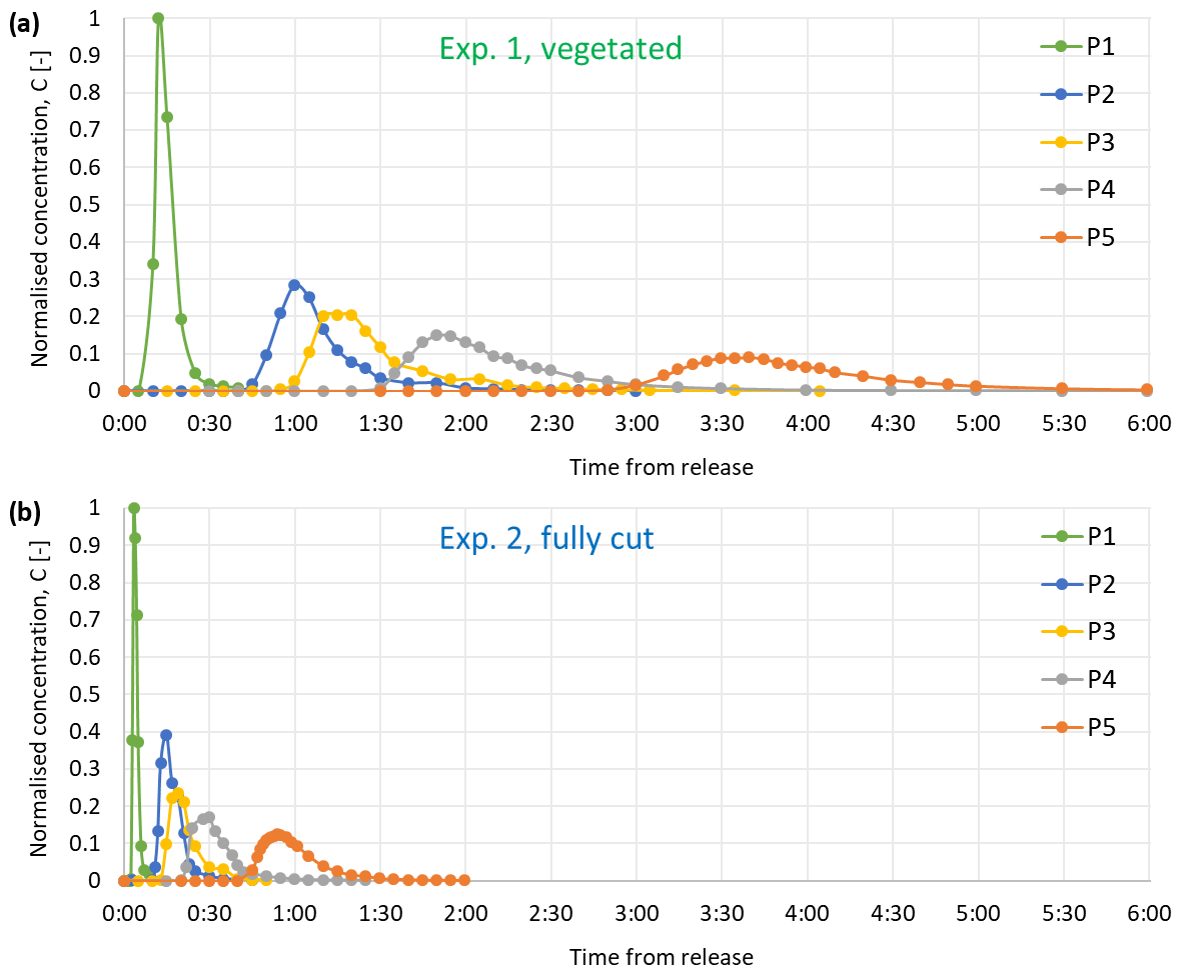
Figure 7 Tracer concentrations in the five cross-sections (P1–P5) normalised with the maximum concentration in the first cross-section P1: (a) vegetated conditions (Exp. 1) and (b) fully cut conditions (Exp. 2).

Values of the recorded peak travel time (t_p) and normalised peak concentration (C_max) as well the computed values of the centroid travel time (t_c) and variance of temporal concentration distributions (σ²) for all cross-sections are summarised in Table 2. The obtained vegetation coverage and parameters describing flow and mixing based on the tracer data are summarised in Table 3 separately for each of the four sub-reaches and the entire channel reach. Both travel times have been plotted depending on the distance from the release point in Fig. 8. As expected, t_p was shorter than t_c in both scenarios. Both t_p and t_c were shorter in the cut conditions. The mean sub-reach centroid travel times (T_c) obtained for each sub-reach and the entire reach (Table 3) indicated that the transport of the dye plume was 3–5 times faster in the case of the fully cut scenario, with larger relative reductions in the travel times observed for the sub-reaches with a higher decrease in the vegetation coverage. The variance of the concentration distributions for both experiments are plotted against the centroid travel time in Fig. 9. Please note that in the case of sub-reach A investigated in fully cut conditions (Exp. 2), the obtained values may be affected by a non-complete mixing over the channel width in the cross-section P1.

Table 2 Tracer data obtained for measured cross-sections (P1–P5) with (Exp. 1) and without (Exp. 2) vegetation.

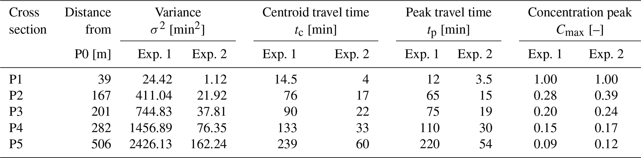
Table 3 Vegetation coverage and parameters describing flow and mixing based on the tracer data for four sub-reaches and the entire analysed reach of the channel during the experiments with (Exp. 1) and without (Exp. 2) vegetation.

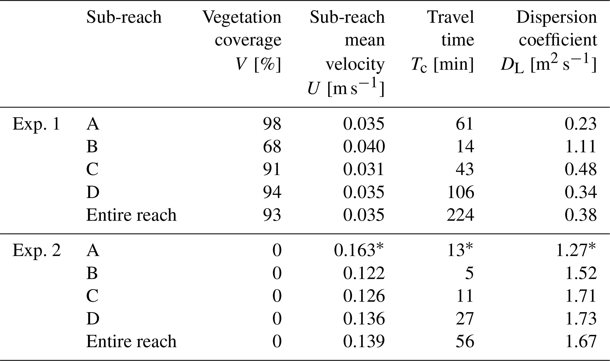
^* Values affected by not-well mixed conditions over the channel width in the P1 cross-section.

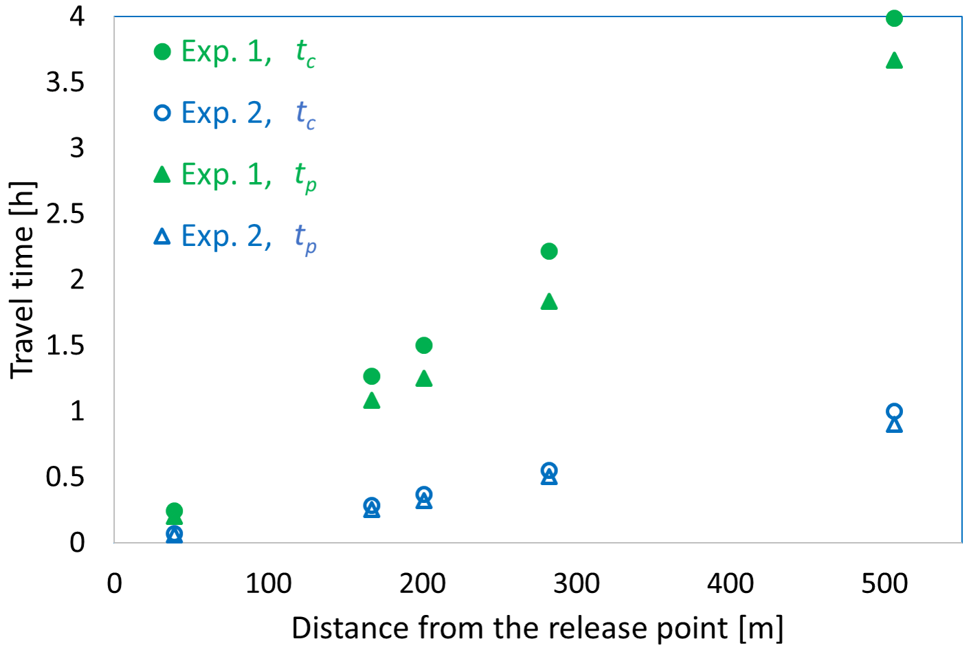
Figure 8 Centroid t_c and peak travel time t_p during the experiments in vegetated (Exp. 1) and fully cut (Exp. 2) conditions.

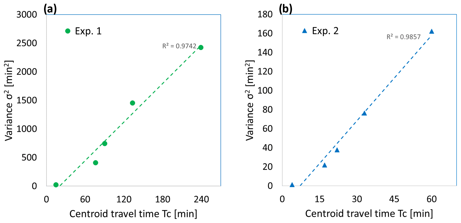
Figure 9 Variance (σ²) of the temporal concentration distributions against the centroid travel time (T_c) during (a) Exp. 1 and (b) Exp. 2.

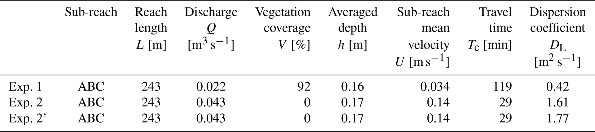
The short duration of the entire experiment in conditions without vegetation allowed for additional control measurements to be carried out. The obtained concentration distributions in the repeated tracer test Exp. 2' were in good agreement with those during the original experiment Exp. 2 (see Fig. A1 and Table A1 in the attachment), confirming constant flow conditions and sufficient accuracy of measurements. The biggest discrepancy, although still relatively small (about 10 %), was observed in the dispersion coefficient, which is due to the difference in the calculated variances of concentration distributions, sensitive to small variations in the concentration tails.

Longitudinal dispersion coefficients in natural channels can vary significantly (e.g. Rutherford, 1994; Heron, 2015). Due to the large variety of conditions in rivers and canals, the reported values may differ by several orders of magnitude. Although there are not many datasets available for the longitudinal dispersion coefficients in small natural streams (Heron, 2015), particularly for low flows, the values of the coefficients obtained during both experiments under non-vegetated conditions (from 1.27 to 1.77 m² s⁻¹) are in good agreement with those previously published and collected by Heron (2015).

3.1 Influence of vegetation maintenance on flow hydraulics

The discharge was approximately double and sub-reach mean velocities were 3-4 times higher in the fully cut conditions when compared to the vegetated scenario (see Tables 1 and 3). Before the maintenance, the vegetation coverage was mostly very high (>90 %), except for sub-reach B (68 %). The vegetation coverage computed for the entire reach (i.e. between the P1 and P5 cross-sections) according to Eq. (1) was equal to 93 %. The water depths were comparable between the two scenarios, ensuring that the vegetation coverage was the most significant factor causing differences in other hydraulic and mixing parameters. Thus, the fully cut conditions that reduced the coverage to 0 % notably improved the conveyance, as was expected based on e.g. Baattrup-Pedersen et al. (2018) and Errico et al. (2019). The increase in the velocity ratio U_NV/U_VEG was approximately linearly dependent on the vegetation coverage (Fig. 10). If we assume that $U_{\mathrm{NV}}/U_{\mathrm{VEG}}=\mathrm{1}$ when V=0, linear regression analysis indicates that under study conditions, the influence of the vegetation cut on the flow velocity can be approximated as $U_{\mathrm{VEG}}=U_{\mathrm{NV}}/(\mathrm{0.03}V+\mathrm{0.9})$. The formula remains the same (considering the coefficients' accuracy to two decimal places) if we include additional data points for vegetation coverage and sub-reach mean velocity, computed using Eqs. (1) and (3), respectively. Additional points (green triangles in Fig. 10) include the values obtained for the entire reach (called the ABCD sub-reach) and selected from possible combinations of sub-reaches, i.e. ABC (P1–P4) and BC (P2–P4). The ABC and BC sub-reaches were selected as having the computed V differing the most from the already plotted points, equal to 92 % and 85 %, respectively. We assume that the linear dependency between velocity change and vegetation coverage can be extended as a first-order approximation to other trapezoidal channels with such high vegetation coverages > ∼68 %. However, the slope coefficient of the formula likely depends on channel geometry and flow forces, and the formula should be evaluated against a substantially larger dataset to derive more general conclusions. It should be emphasised that the dependency may deviate from the linear relationship at coverages lower than the ones presently investigated.

Figure 10 Ratio of sub-reach mean velocities between non-vegetated (U_NV) and vegetated conditions (U_VEG) as a function of the vegetation coverage (V).

We are not aware of previous studies explicitly quantifying the relationship between the mowed vegetation coverage and enhanced conveyance. However, qualitatively similar results can be inferred from Biggs et al. (2021), who reported an approximately doubled mean velocity when vegetation coverage was reduced from ∼80 % to 0 %, and from Verschoren et al. (2017), who found that vegetation removal from the coverage of 90 % to 0 % decreased flow resistance to one fourth, indicating a substantially enhanced mean velocity. Since the vegetation, in our case, was mostly emergent, the planform and cross-sectional blockage by vegetation are approximately similar, indicating that the results are in line with studies reporting a strong relationship between flow resistance and the cross-sectional vegetative blockage (e.g. Green, 2005; Nikora et al., 2008). However, as common for field conditions, it was not possible to control all the variables that may influence the flow discharge in a channel. Besides the major influence of vegetation removal on the results, some impacts may come from other origins. Water depth was somewhat lower, particularly in the two most downstream sub-reaches in Exp. 2 compared to Exp. 1, which partly explains why the flow velocity increased more than the discharge (Table 3 vs. Table 2). The reported flow velocities based on the tracer data may slightly differ from the mean velocity classically determined as discharge divided by flow area (e.g. due to the low number of measured cross-sections and not well-mixed conditions). The presented image analysis method may not recognise very small patches or submerged vegetation and is not directly applicable to such conditions.

3.2 Influence of vegetation coverage on longitudinal dispersion

Table 3 shows longitudinal dispersion coefficients (D_L) for each sub-reach and for the entire reach. Similarly to the flow velocities, the longitudinal dispersion coefficient values were significantly higher in the second experiment (fully cut conditions) compared to the vegetated conditions (see Fig. 11). The highest values of U and D_L under vegetated conditions were found for the least vegetated area, i.e. sub-reach B.

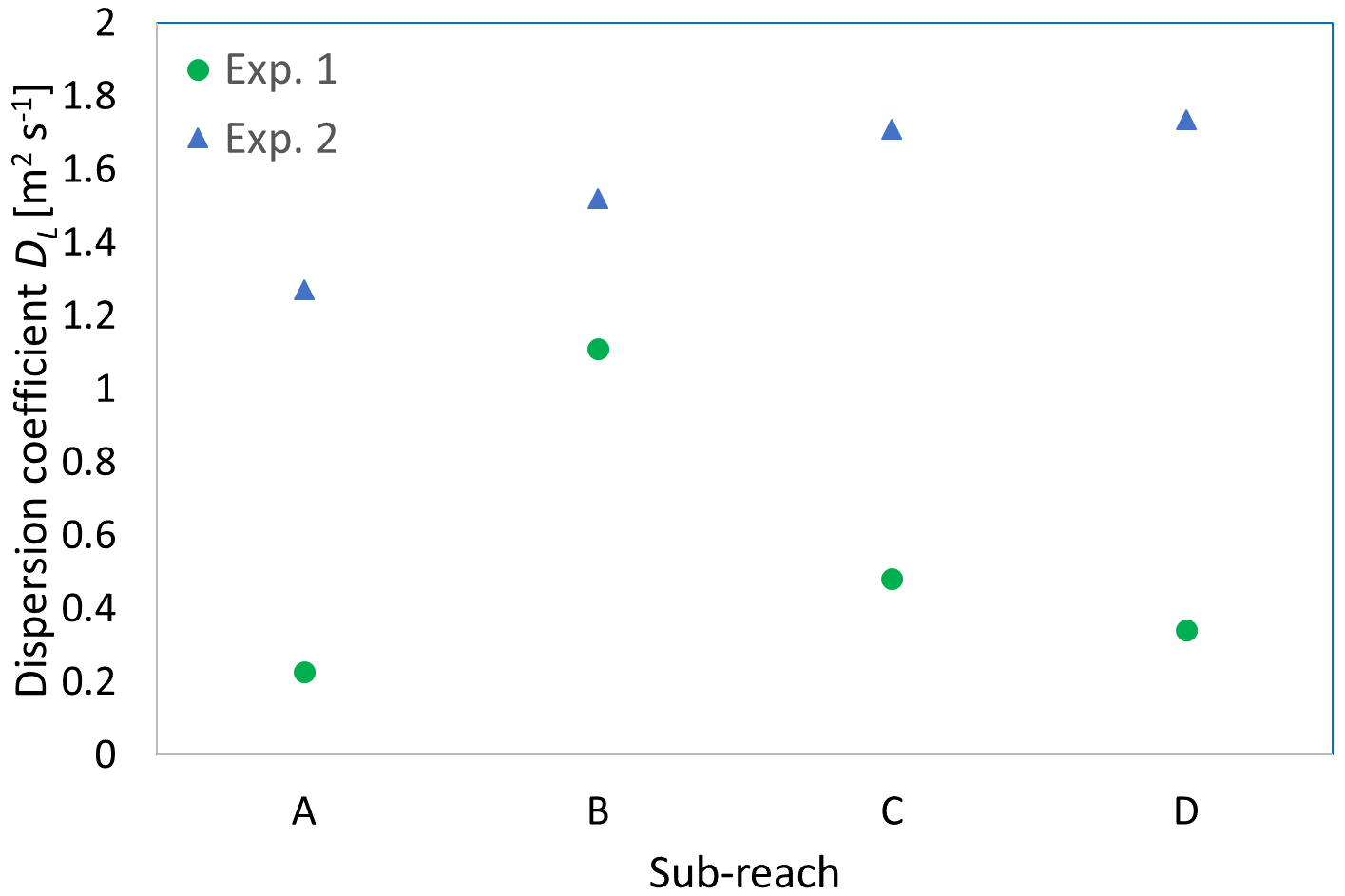
Figure 11 Longitudinal dispersion coefficient (D_L) in vegetated (Exp. 1) and fully cut (Exp. 2) conditions for each individual sub-reach.

Considering different vegetation coverages in particular sub-reaches in the first experiment, it is worth analysing how change in vegetation coverage affects longitudinal dispersion coefficients. The relationship between obtained longitudinal dispersion coefficient (D_L) and vegetation coverage (V) are presented in Fig. 12. The dispersion coefficients decrease with the increase of the vegetation coverage. The line fitted to the obtained values for each sub-reach (circles) indicates a linear relation in the analysed range of vegetation coverage.

Similarly to the velocity ratio, the additional values may be computed for the entire reach ABCD and chosen sub-reaches: ABC and BC. The obtained values of dispersion coefficients are 0.38, 0.42, and 0.61 m² s⁻¹ for the entire 467 m long reach and for the ABC and BC sub-reaches, respectively. These additional values of D_L and V are added to Fig. 12 (green triangles) and they lie close to the line fitted to the previously obtained points (circles).

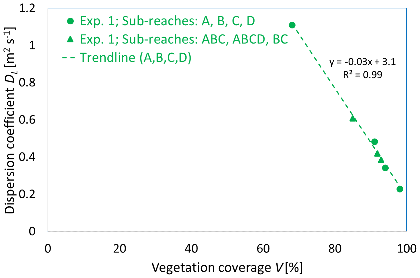
Figure 12 Longitudinal dispersion coefficient (D_L) depending on the vegetation coverage (V) in fully vegetated conditions (Exp. 1).

In non-vegetated open-channel flows, mixing parameters are often scaled against bed shear stress and water depth (e.g. Fischer, 1975; Wang and Huai, 2016), allowing for comparison of non-dimensional dispersion coefficients for different flow rates. However, the applicability of the traditional scaling of the longitudinal dispersion coefficient by the shear velocity for the vegetated flows is debatable. In artificially vegetated conditions, this is no longer appropriate, as the bed is not the dominant source of turbulence (Shucksmith et al., 2010). Therefore, despite different attempts and investigations under laboratory conditions (e.g. Lightbody and Nepf, 2006; Murphy et al., 2007), D_L scaling in naturally vegetated channels remains an open question. The problem is incredibly complex in small natural streams with very diverse, extensive vegetation. Large datasets from further observations for different flow conditions, including detailed hydrodynamic measurements, are needed to address this question. However, to compare the data obtained from both experiments, we scaled the D_L coefficient values against the mean sub-reach velocity (U) values for each experiment (Fig. 13). In the case of Exp. 1, the value of the D_L scale against the U decreases with the increase of the vegetation coverage V, similar to that presented in Fig. 12. In the case of Exp. 2, except for the value obtained for the sub-reach A (affected by non-well mixed conditions over the channel width in the P1 cross-section), the obtained values of $D_{\mathrm{L}}/U$ are comparable for the B, C, and D sub-reaches ($\approx \mathrm{13}\pm \mathrm{0.6}$ m). The obtained results suggest that although we may expect a linear relationship between the vegetation coverage and dispersion coefficient for highly vegetated conditions, the relation may be different for channels with low vegetation coverage.

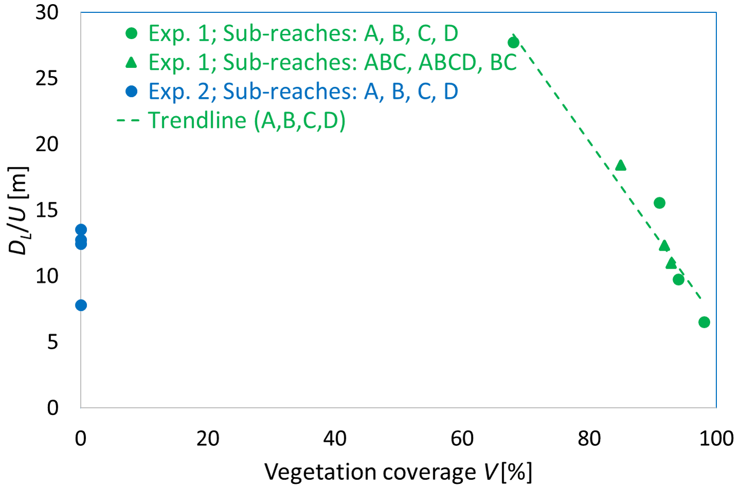
Figure 13 Longitudinal dispersion coefficient D_L scale against the mean sub-reach velocity U depending on the vegetation coverage (V).

The present values of dispersion coefficients and their relation with the vegetation coverage agree with previous findings obtained with uniform vegetation (e.g. Nepf et al., 1997; Shucksmith et al., 2010) confirming that the presence of high vegetation coverage can diminish longitudinal dispersion. Our study shows that the decreasing effect of plants on dispersion extends from fully vegetated conditions down to the vegetation coverage of $\mathrm{2}/\mathrm{3}$. As past investigations (Pan et al., 2019; Västilä et al., 2022) found that the dispersion can increase at lower coverages, particularly if the vegetation clumps, further experiments are needed to confirm the present conclusions and extend the obtained relationship to vegetation coverage below 68 %, as well as considering different vegetation arrangements and various flow conditions.

3.3 Implications of vegetation maintenance on pollutant management

The vegetation cutting that reduced the coverage from 68 %–98 % to 0 % substantially influenced the flow and transport processes. The mean flow sub-reach velocity increased by about 3–4 times and the passage of the concentration peak was 4–5 times faster (see Fig. 8), while the mean water levels remained comparable. In addition, the cutting moderately increased the peak concentrations (Fig. 7). Thus, extensive cutting of vegetation can lead to harmfully high concentrations in small agricultural channels receiving large inputs of nutrients and agricultural chemicals from the fields. The fast flushing of the contaminants to receiving downstream water bodies is exacerbated by sub-surface drainage, typically used in northern and central Europe, which creates very flashy hydrographs (e.g. Västilä and Järvelä, 2011). The limited residence times under non-vegetated conditions (Fig. 7) decrease the likelihood for instream retention and may manifest as increased nitrate (Soana et al., 2019) and suspended sediment loads (e.g. Biggs et al., 2021; Rasmussen et al., 2021) to downstream water bodies after extensive cutting. In addition to decreasing instream retention, vegetation removal may increase erosion and mobilisation of e.g. heavy metals and phosphorus from the channel bed (Old et al., 2014).

The relative changes were lower for the smaller reduction in vegetation coverage, suggesting that less extensive vegetation removals create less severe impacts on the transport of harmful substances while substantially enhancing the flow conveyance (Fig. 10). Leaving some vegetation in the channel, e.g. close to the banks (Errico et al., 2019), likely guarantees acceptable water levels while allowing solutes and particulate matter to have a longer time to be permanently trapped or processed into less harmful forms. There is a need to evaluate the impacts of less intensive cutting scenarios, such as different spatial patterns of cutting and heights of vegetation, and of different channel designs and geometries (e.g. Bal et al., 2011; Västilä et al., 2016) on transport and mixing. In addition, the most suitable timing of cutting based on different criteria should be accurately determined, as Baattrup-Pedersen et al. (2018) observed that the conveyance enhancement by summertime cutting of aquatic vegetation could be short term.

4 Conclusions

In small agricultural channels, water, sediments, and pollutants can flow quickly and be present in relatively high concentrations. The fate of these substances is likely further influenced by the common practice of annually cutting the channel vegetation. In the case of vegetated conditions (in comparison to non-vegetated ones), velocities and concentrations are generally lower. Additionally, pollutant concentrations may be further diminished by vegetation that also serves as a filter and trap for different substances. Nevertheless, water always passes downstream. Therefore, improving our understanding of the hydraulics and mixing in small vegetated channels is crucial for predicting water quality at the catchment scale including downstream water bodies.

Our study on the influence of vegetation maintenance on hydraulics and mixing in a real agricultural channel is novel in that a wide range of initial vegetation coverages from $\sim \mathrm{2}/\mathrm{3}$ to 1 was experimented. Most previous work has focused on fully vegetated flows or is limited to specific well-defined laboratory conditions, often with artificial plants. The present results confirm that natural vegetation at large coverages diminishes the longitudinal dispersion coefficient, and indicate that relation between the vegetation coverage and dispersion coefficient is linear at the investigated vegetation coverage > 68 %. The obtained results are limited to high vegetation coverage conditions and should be complemented by observations performed with different hydrological and vegetational conditions.

The investigations showed that a series of relatively simple 1D analyses could help to study the influence of vegetation maintenance scenarios on flow and mixing in small agricultural channels. In addition, they are useful for finding generalisable relationships between longitudinal dispersion coefficient, flow hydraulics, and vegetation coverage in small channels. Such relationships are expected to be helpful for practitioners in optimising vegetation maintenance, considering both flow conveyance and water quality.

Additional studies are needed to determine how different vegetation maintenance regimes influence mixing and retention. These experiments should consider various conditions, including many flow variants, less intensive coverage, different vegetation arrangements, and the stage of plants, which may be changed by manual conservation practice or seasonal growth. Such data will allow us to combine different viewpoints in managing channels to effectively promote the flow conveyance and the local biodiversity and the retention of nutrients and pollutants.

Using a case study in Poland, our dataset provides a valuable reference for further investigations as it complements the existing databases, which are generally not focused on small streams (e.g. Sukhodolov et al., 1997; Heron, 2015) and are barely available for vegetated natural streams. In the face of a small number of studies in natural vegetated conditions, the results linking D_L with V are useful and help in designing more detailed future investigations.

Appendix A: Repetition of experiment under non-vegetated condition

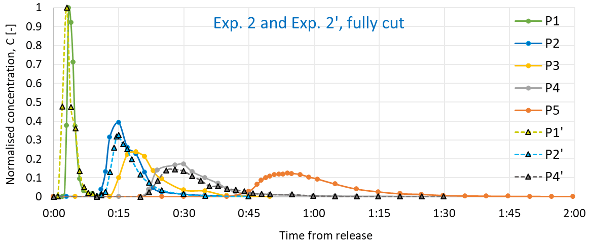
Figure A1 Tracer concentrations in measured cross-sections normalised with the maximum concentration in the first cross-section P1. Fully cut conditions, original Exp. 2 (cross-sections P1, P2, P3, P4 and P5) and repeated experiment Exp. 2' (cross-sections P1', P2' and P4').

Table A1 Hydraulic, vegetative and mixing parameters of the sub-reach between the P1 and P4 cross-sections during the experiments in vegetated (Exp. 1) and in fully cut conditions – original (Exp. 2) and repeated experiment (Exp. 2').