the Creative Commons Attribution 4.0 License.
the Creative Commons Attribution 4.0 License.
 | 28 Feb 2023
Hydrological modeling using the Soil and Water Assessment Tool in urban and peri-urban environments: the case of Kifisos experimental subbasin (Athens, Greece)
Evgenia Koltsida
Nikos Mamassis
Andreas Kallioras
SWAT (Soil and Water Assessment Tool) is a continuous-time, semi-distributed, river basin model widely used to evaluate the effects of alternative management decisions on water resources. This study examines the application of the SWAT model for streamflow simulation in an experimental basin with mixed-land-use characteristics (i.e., urban/peri-urban) using daily and hourly rainfall observations. The main objective of the present study was to investigate the influence of rainfall resolution on model performance to analyze the mechanisms governing surface runoff at the catchment scale. The model was calibrated for 2018 and validated for 2019 using the Sequential Uncertainty Fitting (SUFI-2) algorithm in the SWAT-CUP program. Daily surface runoff was estimated using the Curve Number method, and hourly surface runoff was estimated using the Green–Ampt and Mein–Larson method. A sensitivity analysis conducted in this study showed that the parameters related to groundwater flow were more sensitive for daily time intervals, and channel-routing parameters were more influential for hourly time intervals. Model performance statistics and graphical techniques indicated that the daily model performed better than the subdaily model (daily model, with NSE = 0.86, R2 = 0.87, and PBIAS = 4.2 %; subdaily model with NSE = 0.6, R2 = 0.63, and PBIAS = 11.7 %). The Curve Number method produced higher discharge peaks than the Green–Ampt and Mein–Larson method and better estimated the observed values. Overall, the general agreement between observations and simulations in both models suggests that the SWAT model appears to be a reliable tool to predict discharge in a mixed-land-use basin with high complexity and spatial distribution of input data.
- Article
(3267 KB) - Full-text XML
- BibTeX
- EndNote


Water resource problems, including the effects of urban development, alternative management decisions, and future climate oscillation on streamflow and water quality, require a deep understanding and accurate modeling of Earth surface processes at the catchment scale to be addressed (Gassman et al., 2014). In order to understand catchment processes, it is necessary to obtain detailed weather data and catchment observations related to runoff, water stage, erosion, soil moisture, and water quality. Experimental catchments are properly designed and well-monitored catchments that aim to provide databases of long-term historical hydrological data, which help analyze the mechanisms governing surface runoff (Goodrich et al., 2020). In addition, experimental catchments contribute to the development and validation of numerous watershed models and can be used as validation sites for satellite sensors (Tauro et al., 2018). Furthermore, experimental catchments monitor groundwater and river water quality with the use of tracer experiments which can estimate the residence and travel times of water in different components of the hydrological cycle (Hrachowitz et al., 2016; Stockinger et al., 2016). Bogena et al. (2018) presented an extensive overview of hydrological observatories presently operated worldwide under various environmental conditions. Among those, the U.S. Department of Agriculture Agricultural Research Service's (USDA-ARS) Experimental Watershed Network has operated over 600 watersheds in its history and currently operates more than 120 experimental hydrological watersheds (Goodrich et al., 2020).
Hydrological and water quality models have been widely used to assess water resource problems and to investigate hydrological processes, land use and climate change impacts, and best management practices (Daggupati et al., 2015). In recent decades, various watershed-scale models (i.e., SWAT, APEX, HSPF, WAM, KINEROS, and MIKE-SHE) have been developed to operate with different levels of input data and model structure complexity (Arnold et al., 2015; Moriasi et al., 2007). Among the above watershed-scale models, the SWAT program (Soil and Water Assessment Tool; Arnold et al., 2012) was selected for this study. SWAT is a physically based, semi-distributed, continuous-time river basin model and has five main official versions, namely SWAT2000, SWAT2005, SWAT2009, SWAT2012, and SWAT+. It was selected because it is an open-source code, has a wide range of online documentation and a literature database, and has been applied to catchments of various sizes and several temporal scales (e.g., monthly, daily, and subdaily time steps; Gassman et al., 2007, 2014; Tan et al., 2020). Furthermore, it can be linked to QGIS, also a free and open-source platform, and has the ability to visualize the results, which can be helpful for the interpretation of the many SWAT outputs (Dile et al., 2016).
SWAT has two methods for the estimation of surface runoff, namely the SCS Curve Number (CN) method (Soil Conservation Service, 1972) for daily rainfall and the Green–Ampt and Mein–Larson infiltration (GAML) method (Mein and Larson, 1973) for subdaily rainfall. The CN method has been used more often than the GAML method in SWAT model applications, mainly due to the absence of high temporal-resolution data needed for the subdaily module (Bauwe et al., 2016; Brighenti et al., 2019; Gassman et al., 2014). The few available studies suggest that the calibrated streamflow results are more accurate when using the CN approach compared to the GAML approach (Bauwe et al., 2016; Cheng et al., 2016; Ficklin and Zhang, 2013; Kannan et al., 2007). In particular, in the study in which CN improved the results, Kannan et al. (2007) identified a suitable combination of evapotranspiration and runoff-generation methods and reported that the CN method performed better than the GAML method. In contrast, three studies reported that the GAML method simulated the peak flows during the flood season better than the CN method (Li and DeLiberty, 2020; Maharjan et al., 2013; Yang et al., 2016). Some studies have pointed out that both approaches have limitations and that the improvement depends on the part of the hydrograph that is analyzed (e.g., high, medium, or low flows) in addition to the timescale (e.g., daily, monthly, or annually; Han et al., 2012; King et al., 1999). Furthermore, several subdaily applications have been conducted, such as land use and management impacts on flood events (Golmohammadi et al., 2017; Campbell et al., 2018), the use of high temporal-resolution data for the improvement of the model (Bauwe et al., 2017; Boithias et al., 2017), and modeling of rainfall–runoff events (Jeong et al., 2010; Yu et al., 2018). The authors generally found that finer temporal-resolution time steps do not always improve model performance but depend on the basin scale and the characteristics of the watershed. A detailed description of the model history and applications can be obtained in Gassman et al. (2007), Douglas-Mankin et al. (2010), Brighenti et al. (2019), and Tan et al. (2020).
The selected study area has been severely urbanized from 1990 until today, at the expense of forests and agricultural areas. During this period, the artificial surfaces increased by 69.93 %, and the agricultural areas and the forests decreased by 54.14 % and 14.34 %, respectively (CORINE Land Cover, CLC 1990–2018). The area is portrayed as an urban/peri-urban system with about 51 % of artificial surfaces, 13 % of agricultural areas, and 36 % of forests and semi-natural areas. The interaction between different land uses (e.g., urban and rural characteristics) contributes to the formation of a complex environment characterized by high variability in management practices, rapid response, and diverse hydrological processes, which may increase problems in model uncertainties (Boithias et al., 2017). Land use maps and soil maps may not capture this complex environment precisely, enhancing the SWAT model's difficulty in representing and simulating the actual conditions of the basin, which can affect water discharge. In addition, the study area is a typical Mediterranean catchment that is vulnerable to natural hazards (i.e., flash floods and forest fires). In order to interpret the behavior of such a complex environment, the SWAT 2012 hydrological model (rev. 681) was used for its realistic representation. The available studies that used the subdaily option of the SWAT model refer mainly to agricultural (Bauwe et al., 2016; Boithias et al., 2017; Cheng et al., 2016; Ficklin and Zhang, 2013; Golmohammadi et al., 2017; Maharjan et al., 2013; Yang et al., 2016; Yu et al., 2018) or small urban catchments (Campbell et al., 2018; Jeong et al., 2010; Li and DeLiberty, 2020) and rarely to peri-urban catchments. Thus, the suitability of the subdaily option of the SWAT model to simulate discharge in a peri-urban catchment has not been extensively tested. The main objectives were (i) to investigate which parameters are more sensitive under different time steps in a mixed-land-use basin (i.e., blended combinations of land use, management practices, and hydrological processes), (ii) to compare the results of the hourly time step simulation (Green–Ampt and Mein–Larson method) to those obtained from daily time step simulation (Curve Number method), and (iii) to evaluate the subdaily option of the SWAT model for discharge simulation by examining peak discharges and time of the peak of selected rainfall events. The calibration methodology developed in this catchment can be applied to areas with similar hydrological–meteorological and geomorphological attributes (i.e., Mediterranean peri-urban areas). This study provides essential hydrological knowledge and contributes to understanding the critical processes of an urban/peri-urban system to analyze the mechanisms governing surface runoff at the catchment scale. The outcomes will establish a basis for further modeling applications, which will be helpful for local planners to use in future regional urban development strategies. The study area information, methodology, and data input are presented in Sect. 2, results and discussions are detailed in Sect. 3, and the conclusion is provided in Sect. 4.
2.1 Study area
The study area includes the upper part (NW subbasin) of the Kifisos river basin, located in Athens, Greece (Fig. 1a). The Kifisos river basin occupies an area of 380 km2. The Kifisos river route is approximately 22 km, of which at least 14 km is within an urban area. The elevation ranges from 94 to 1399 m, with plains in the south and hills in the northern part of the basin. The mean annual temperature is 16.4 ∘C, and the mean annual rainfall across the basin is 577.2 mm.
The study area is characterized as an urban/peri-urban area, with residential areas, shrubland, and agriculture accounting for 34.1 %, 15.9 %, and 12.4 % of its land use coverage, respectively (Fig. 1b). It includes mainly four soil types, i.e., Cambisols, Regosols, Leptosols, and Luvisols (Fig. 1c). The dominant soil formations are characterized by good soil permeability and high contents of clay and sand.
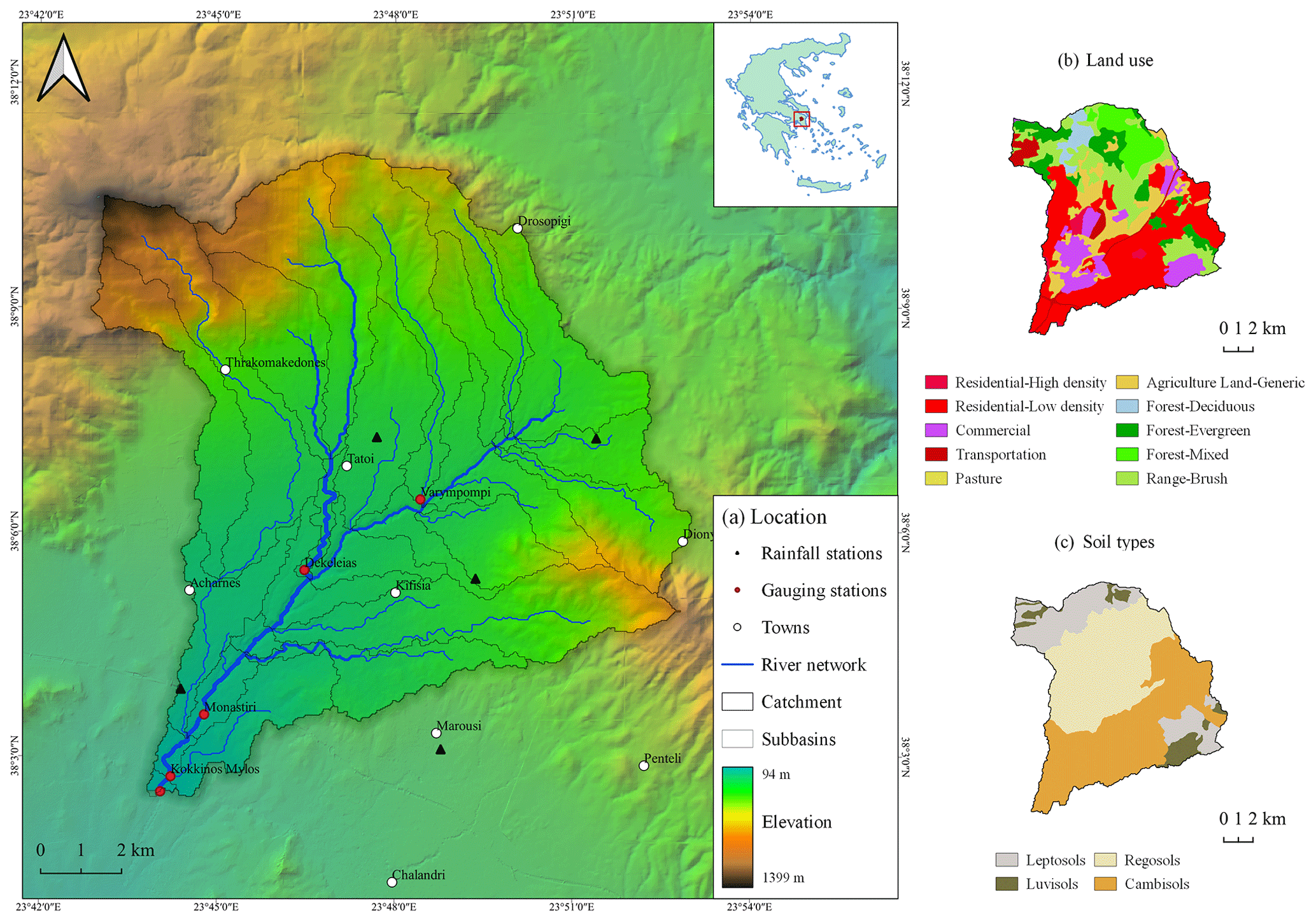
Figure 1Geographical location of the study area (a) and spatial distribution of land use (b) and soil (c).
2.2 Experimental catchment of Athens metropolitan area
The study area includes four water-level monitoring stations that provide continuous recordings of the river stage at preselected time intervals (15 min time step; Fig. 1). The stations were installed at the end of 2017 under the supervision of the School of Mining at the National Technical University of Athens (NTUA). The network was developed under the European Union Horizon 2020 Research and Innovation Action (RIA) program of SCENT (Smart Toolbox for Engaging Citizens in a People-Centric Observation Web). The station located at the outlet of the study area was selected as the most suitable for further analysis in this study because the three upstream stations experienced some mechanical problems that affected the calibration and validation process. The monitoring stations are part of the Open Hydrosystem Information Network (https://OpenHi.net, last access: 20 December 2020), which is a national integrated information infrastructure for the collection, management, and free dissemination of hydrological data (https://OpenHi.net, last access: 20 December 2020) in Greece.
2.3 Data sources
The input data for the construction of the SWAT model include a digital elevation model (DEM), a land use map, a soil map, and meteorological data (i.e., rainfall, temperature, wind speed, relative humidity, and solar radiation). Table 1 summarizes the input data and their sources used in this study.
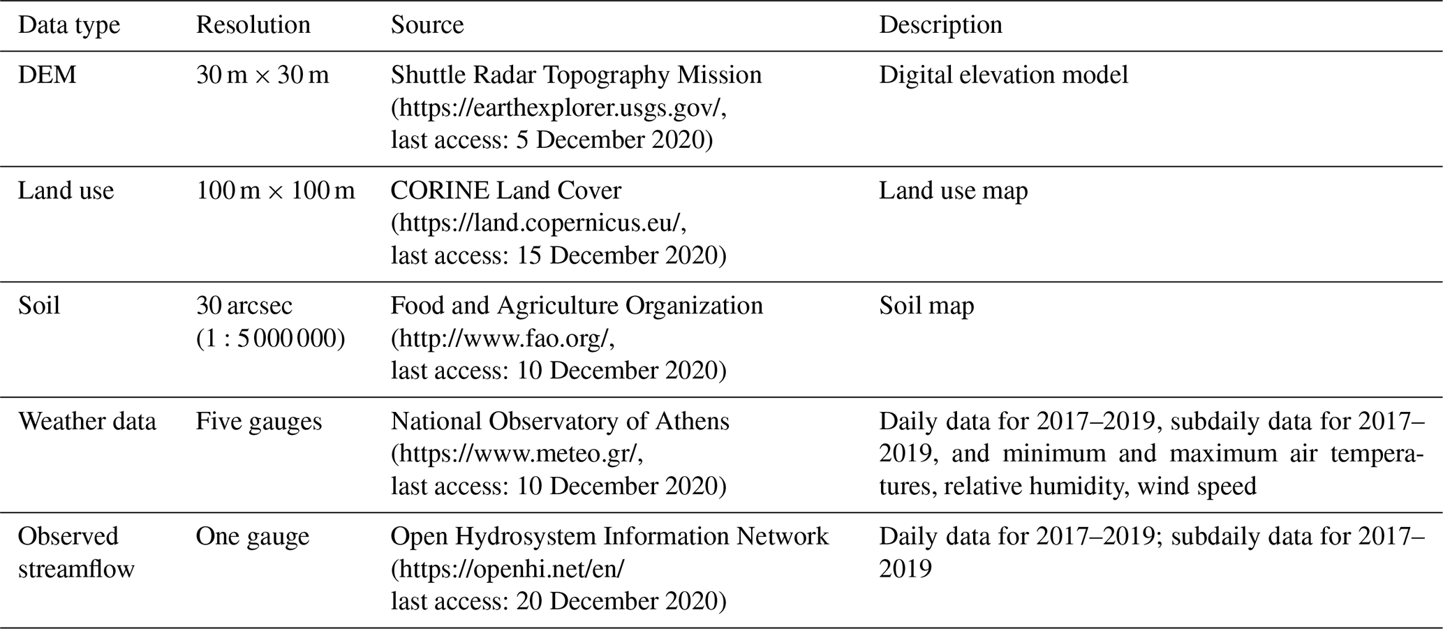
Table 2Land use classification of the Kifisos basin and the corresponding SWAT land use category.
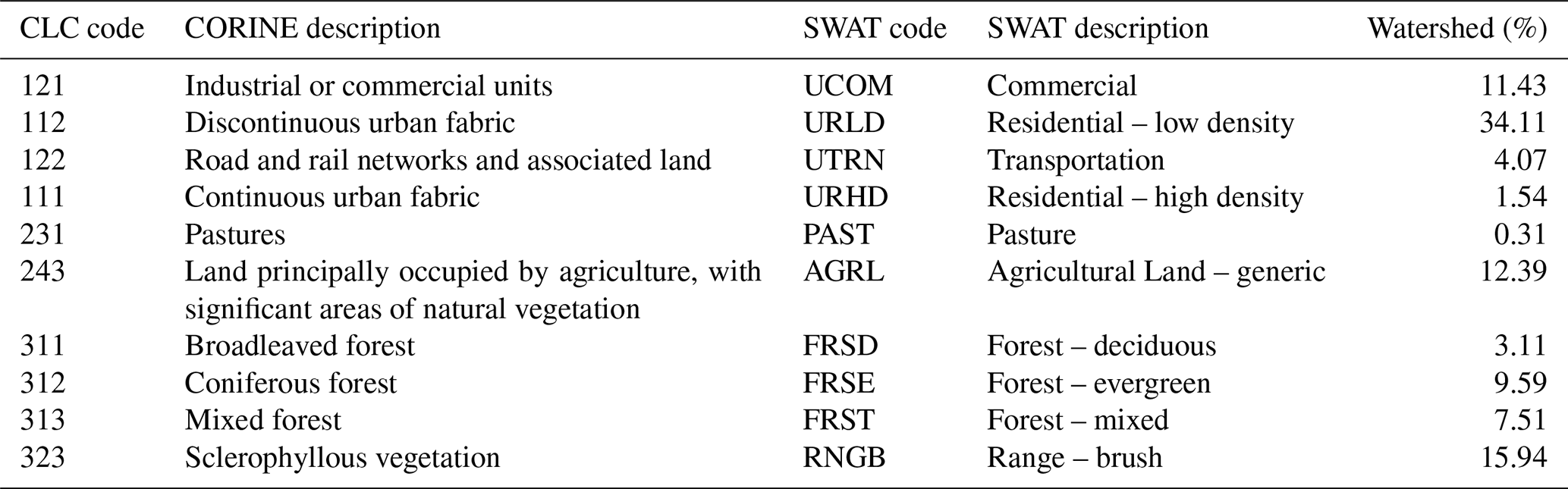
The digital elevation model (DEM) at 30 m spatial resolution was downloaded from the website of the U.S. Geological Survey (USGS). The land use map was derived from the 100 m 2018 CORINE Land Cover map (CLC, 2018) and was modified according to SWAT land use categories (Table 2). The soil map was created from data from the Food and Agriculture Organization (FAO) Digital Soil Map of the World (FAO et al., 2012). In addition, rainfall data, relative humidity, wind speed, and the minimum and maximum air temperature were obtained from the National Observatory of Athens (NOA). Solar radiation data were simulated by WGEN, a weather generator developed by SWAT to fill the missing meteorological data using monthly statistics. A rain gauge network consisting of five gauges is distributed throughout the study area, as illustrated in Fig. 1. Daily and hourly (Δt = 1 h) rainfall data were retrieved from 2017 to 2019, with coverage during the entire year. The daily and subdaily observed streamflow data at the basin outlet (Fig. 1) from 2017 to 2019 were acquired from the Open Hydrosystem Information Network (https://OpenHi.net, last access: 20 December 2020).
2.4 Soil Water Assessment Tool (SWAT)
The SWAT (Soil and Water Assessment Tool) program is a semi-distributed, continuous-time, process-based model (Arnold et al., 1998, 2012). The model operates on a daily time step, and it has been recently updated to subdaily time step computations (Jeong et al., 2010). SWAT has been developed to evaluate the impact of management practices on water, sediment, and agricultural chemical yields in large river basins over long time periods. The main components of SWAT are hydrology, weather, soil properties, land use, crop growth, sediments, nutrients, pesticides, bacteria, and pathogens.
In SWAT, a watershed is divided into multiple subbasins, which are then subdivided into hydrologic response units (HRUs) based on unique soil, slope, and land use attributes. HRUs enable the model to represent differences in evapotranspiration for various vegetation and soil types. Simulation of the hydrology of a watershed can be separated into the land phase, which determines the loadings of water, sediment, nutrients, and pesticides to the main channel, and the routing phase, which is the movement of the loadings through the streams of the subbasins to the outlets (Neitsch et al., 2011).
Hydrological processes are simulated separately for each HRU, including canopy storage, surface runoff, partitioning of the precipitation, infiltration, redistribution of water within the soil profile, evapotranspiration, lateral subsurface flow from the soil profile, and return flow from shallow aquifers (Gassman et al., 2007). SWAT uses a single plant growth model to simulate all types of vegetation and can differentiate between annual and perennial plants. The plant growth model estimates the amount of water and nutrients removed from the root zone, transpiration, and biomass/yield production.
The main difference between the daily and subdaily simulations in SWAT occurs in the surface runoff estimation. The SCS Curve Number (CN) method (Soil Conservation Service, 1972) is used for daily simulations, and the Green–Ampt and Mein–Larson infiltration (GAML) method (Mein and Larson, 1973) is used for subdaily simulations. The CN method is an empirical, widely used model and requires land use, soil, elevation, and daily rainfall data as input. The GAML method is a physically based model, uses the same spatial coverages as the CN method, and requires more detailed soil information and subdaily rainfall records as input. More details on the model theory, equations, and processes can be found in Arnold et al. (1998), Gassman et al. (2007), and in Neitsch et al. (2011).
2.5 Model setup
The latest version of the SWAT 2012 hydrological model was used in this study. The QSWAT plugin (Dile et al., 2016) embedded in the QGIS platform was used for the setup and the parameterization of the model. The watershed delineation, stream parameterization, and overlay of soil, land use, and slope were automatically completed within the interface. A drainage area of 3.6 km2 was chosen to discretize the study area. The area was delineated into 25 subbasins, which were then divided into 175 HRUs.
The SWAT models for the Kifisos basin include daily and subdaily (hourly) rainfall observations. Potential evapotranspiration was calculated by the Penman–Monteith method, surface runoff was estimated using the CN method for the daily model and the GAML method for the hourly model, and the variable storage coefficient method was used to calculate the channel routing. The simulation period was from 2017 to 2019, and the first year was used as a warmup period to mitigate the unknown initial conditions. The model was calibrated from 1 January to 31 December 2018 and validated from 1 January to 31 December 2019 for discharge using the Sequential Uncertainty Fitting (SUFI-2) program in SWAT-CUP software (Abbaspour et al., 2004, 2007).
2.6 Sensitivity analysis and model calibration and validation
Watershed models are characterized by significant uncertainties related to conceptual design, input data, and parameters (Abbaspour et al., 2015). The model calibration, validation, and uncertainty analysis were achieved with the use of the SUFI-2 algorithm in the SWAT-CUP software (Abbaspour et al., 2004, 2007). In SUFI-2, uncertainties in parameters (e.g., uncertainty in input data, conceptual model, parameters, and measured data) are expressed as ranges or uniform distributions. The concept behind this algorithm is to collect most of the observed data within a narrow uncertainty band. The initial ranges of the calibrating parameters are set based on the literature and sensitivity analyses. Then, parameter sets are generated using Latin hypercube sampling, and the objective function is estimated for each parameter set. The uncertainties are calculated at the 2.5 % and 97.5 % levels of the cumulative distribution of all output variables, and it is referred to as the 95 % prediction uncertainty (95 PPU). The goodness of model performance and output uncertainty is assessed using the P factor and the R factor (Abbaspour et al., 2004). The P factor is the percentage of measured data bracketed by the 95 PPU band, and it ranges from 0 to 1, where 1 means all of the measured data are within the model prediction uncertainty. The R factor is the ratio of the average width of the 95 PPU band and the standard deviation of the measured data. The values of the R factor range from 0 to infinity, where a value near 0 reflects an ideal situation. The spatial scale of the project and the accuracy of the observed data affect the values of the P factor and the R factor (Abbaspour et al., 2015). In this study, the Nash–Sutcliffe (NS) efficiency model was used as an objective function for both daily and subdaily calibration and validation. The sensitivities of the parameters were estimated using the following equation (Eq. 1; Abbaspour et al., 2015):
where g is the goal function, and b's are the parameters selected for calibration. The sensitivities are calculated as the average changes in the objective function which result from changes in each parameter, while all other parameters are changing. A t test is then conducted to evaluate the significance of each parameter bi. Parameters with a large t test value and small P value were characterized as sensitive parameters.
Model validation was achieved using the calibrated parameter ranges without any further changes, and the model performance of the calibration period was compared to the model performance of the validation period. The annual precipitation and daily discharge statistics were calculated for each period to overcome biases in discharge patterns. Annual precipitation for 2018 was 566 mm, and annual precipitation for 2019 was 735 mm. The mean and standard deviation values of discharge for 2018 were 1.25 and 0.46 and for 2019 were 1.42 and 0.74, respectively. These statistics ensure that the selected periods represent both wet and dry conditions. In the calibration and validation process, 18 parameters (Table 3) were used. About 600 simulations per iteration were conducted, and with up to three iterations, until the results of the P factor and R factor were satisfying.
Table 3Daily and subdaily SWAT-calibrated parameters. The method “r” indicates that the parameter value is multiplied by (1 + a given value), the method “v” indicates that the parameter value is going to be replaced, and the method “a” indicates that the parameter is to be added by a given value (Abbaspour et al., 2007).
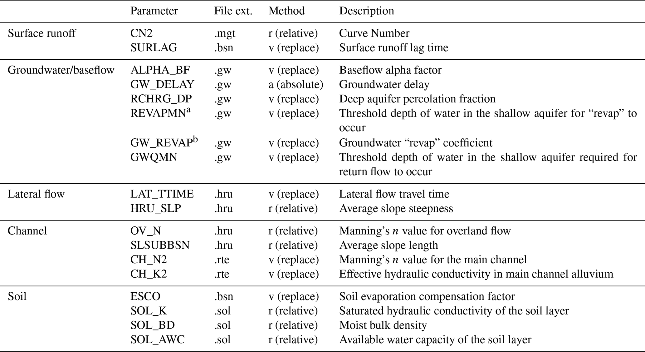
a REVAPMN is the threshold depth of water in the shallow aquifer for evaporation or percolation to occur. b GW_REVAP is the movement of water from the shallow aquifer to the overlying unsaturated zone.
Further evaluation of the model performance was achieved using graphical and statistical techniques (Daggupati et al., 2015b; Harmel et al., 2014; Moriasi et al., 2007, 2015). The most commonly used statistical techniques are the Nash–Sutcliffe efficiency (NSE; Nash and Sutcliffe, 1970), coefficient of determination (R2; Moriasi et al., 2007), and percent bias (PBIAS; Gupta et al., 1999), as shown in Eqs. (2)–(4). The most common graphical techniques are time series charts, scatterplots, bar charts, maps, and percent exceedance probability curves. The statistics were calculated for both models, and then their performance was discussed according to the guidelines (Moriasi et al., 2007, 2015).
where Qobs is the observed discharge, Qsim is the simulated discharge on day i, is the mean of observed discharge, and is the mean of simulated discharge. R2 is a measure of how well the variance of measured data is replicated by the model. R2 can range from 0 to 1, where 0 means no correlation, and 1 indicates a perfect correlation and minor error variance. NSE is a measure of how well the simulated values match the observed values. NSE can range from −∞ to 1, where values ≤ 0 show that the observed data mean is a more accurate predictor than the simulated values, and 1 is a perfect fit between simulated and observed values. Finally, PBIAS measures the average tendency of the simulated values to be larger or smaller than the observed values. The optimum value is 0; positive values show model underestimation, and negative values show model overestimation. More information about the strengths, weaknesses, and usage of the commonly used measures is presented in Moriasi et al. (2015). The SWAT-CUP software is designed mainly for daily, monthly, or annual time steps. In order to calibrate the subdaily model, the SUFI-2 files required minor modifications.
3.1 Parameter's sensitivity analysis and calibration
The most sensitive parameters obtained in daily and hourly simulations are presented in Table 4. Sensitive parameters are characterized by a large t test and small p value. The parameters were characterized as being significantly sensitive when the p value was less than 0.03. In the daily model, the most sensitive parameters were the deep aquifer percolation fraction (RCHRG_DP), groundwater delay time (GW_DELAY), lateral flow travel time (LAT_TTIME), average slope steepness (HRU_SLP), and moist bulk density (SOL_BD). These parameters were connected to groundwater flow, runoff generation, and channel routing. In the subdaily model, the significantly sensitive parameters were average slope steepness (HRU_SLP), Manning's n value for the main channel (CH_N2), effective hydraulic conductivity in the main channel alluvium (CH_K2), and lateral flow travel time (LAT_TTIME). These were all related to channel routing.
Table 4Daily and subdaily SWAT-calibrated parameters and their sensitivities.
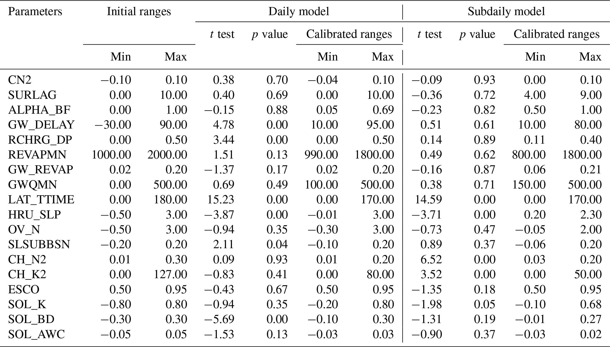
The differences in the sensitivity of the calibrated parameters of the two models reflect the impact of the operational time step on model performance (Boithias et al., 2017; Jeong et al., 2010). In particular, the hourly model is characterized by larger GWQMN and GW_REVAP values than the daily model. GWQMN is the threshold depth of water in the shallow aquifer required for return flow to occur, and GW_REVAP controls the water movement from the shallow aquifer into the overlying unsaturated soil layers. As these parameters increase, the rate of evaporation increases up to the rate of potential evapotranspiration, resulting in a corresponding decrease in the baseflow. Furthermore, the fitted value of CH_N2 in the hourly simulation was 0.11 () and was larger than 0.08 () in the daily simulation. The CH_N2 parameter affects the rate and the flow velocity (Boithias et al., 2017). Therefore, the larger CH_N2 value was connected to a smaller flow velocity. According to Boithias et al. (2017), the CH_N2 parameter is more sensitive at the hourly time step rather than the daily time step because, at the daily time step, the flow peak is influenced by other processes decreasing the sensitivity of the CH_N2. In addition, the value range for CN2 (Curve Number 2) was smaller for the subdaily model, leading to lower peak flows. Other differences were average slope steepness (HRU_SLP), average slope length (SLSUBBSN), groundwater delay time (GW_DELAY), and Manning's n value for overland flow (OV_N). Their values were all smaller in the subdaily simulation. Overall, the differences between the two models lay mainly in the different runoff estimation methods used by the two models.
It is worth noting that the observations, procedures, and assumptions made for this study may affect the results of this study. The values of the calibrated parameters and their sensitivities are influenced by the type and quality of input data, the conceptual model, the choice of the objective function, and inaccuracies in measured input data used for calibration and validation (Abbaspour et al., 2015; Arnold et al., 2012; Polanco et al., 2017).
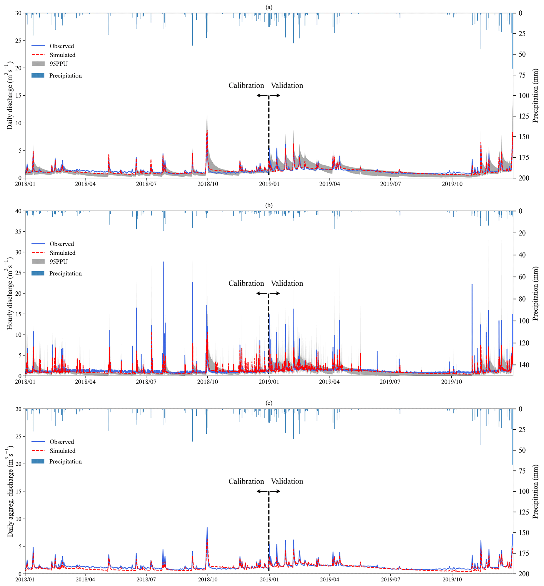
Figure 2Observed and simulated discharge (m3 s−1) during calibration and validation periods. Daily time step (a). Hourly time step (b). Daily time step aggregated from hourly outputs (c). The CN method, with daily rainfall observations, was used for the daily model, and the GAML method, with hourly rainfall observations, was used for the hourly model.
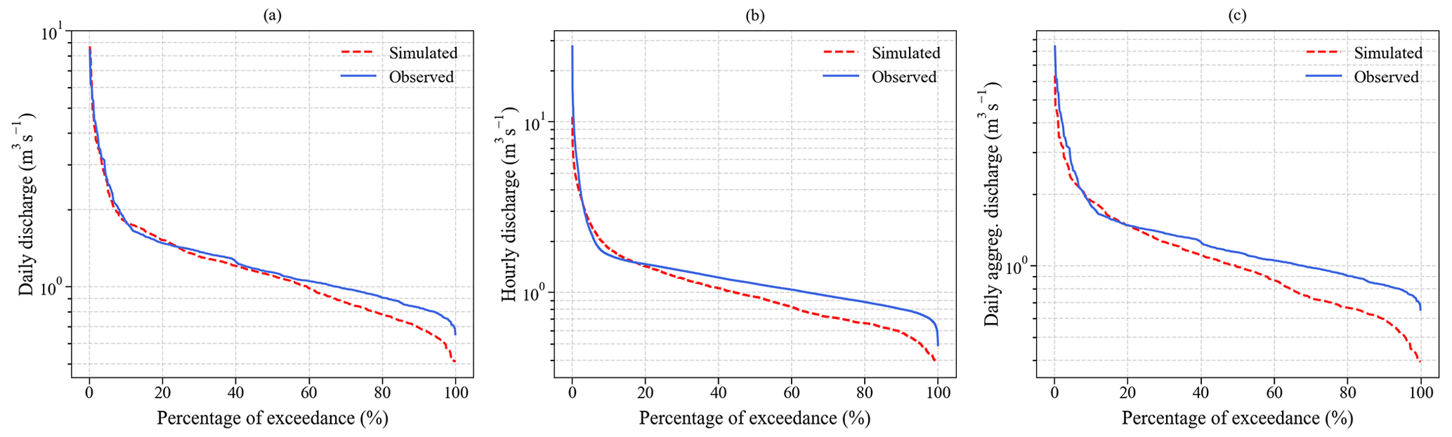
Figure 3Observed and simulated flow duration curves (m3 s−1) at the daily time step (a), at the hourly time step (b), and at the daily discharge aggregated from hourly outputs time step (c).
3.2 Daily and subdaily model performances
Quantitative statistics and criteria recommended by Moriasi et al. (2007, 2015) were used to evaluate the model performance. In order to investigate the influence of rainfall on model performance and compare daily outputs to hourly outputs, the hourly outputs were aggregated to daily averages. Figure 2a and b shows the temporal dynamics of the hydrographs reproduced by both runoff estimation methods. The high-flow season is observed during winter and spring. The low-flow season is observed in summer and early fall due to high evapotranspiration. Figure 2c shows the observed versus the simulated daily discharge aggregated from hourly outputs during the calibration and validation processes. Figure 3 presents the flow duration curves of the models, indicating good agreement between the observed and simulated values. Generally, in the subdaily model, the simulated discharge peaks did not always match the observed values and were sometimes considerably lower.
Table 5Model evaluation statistics of the daily, subdaily, and daily aggregated from hourly output SWAT models for the calibration and validation periods.
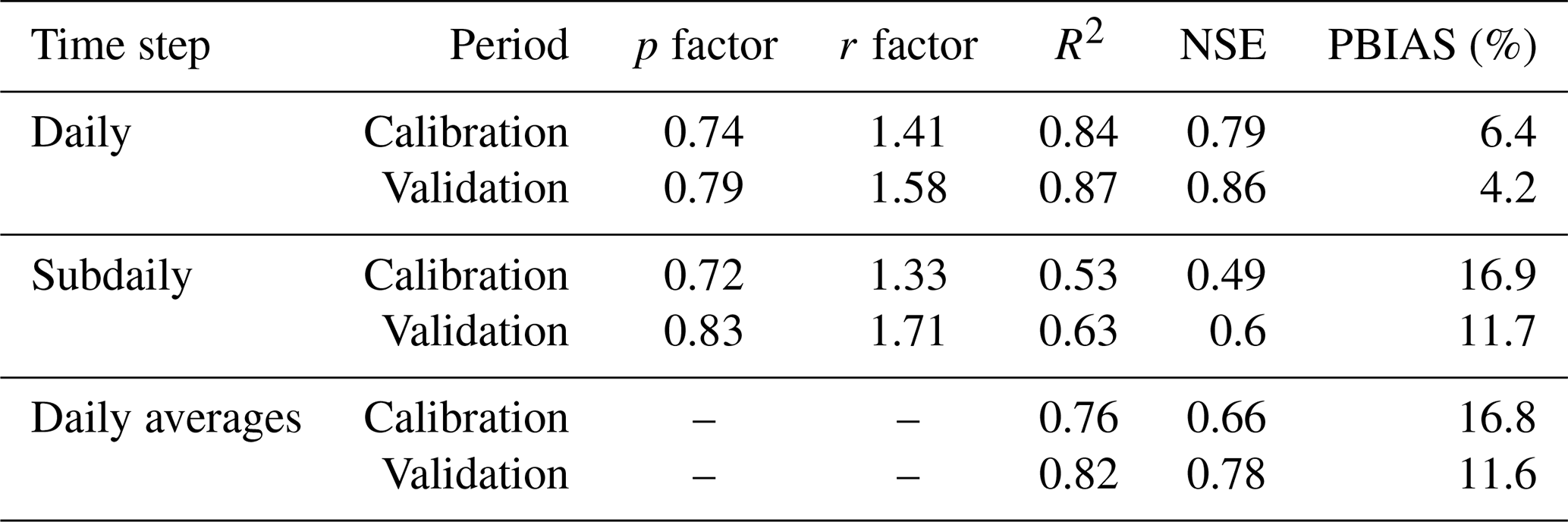
The performance statistics are illustrated in Table 5 and indicate reasonable calibrated models for both methods. Model performance of the daily model using the CN method showed better results than the hourly model using the GAML method. In particular, the NSE and R2 indices for the daily model were 0.84 and 0.79 for the calibration period and 0.87 and 0.86 for the validation period. For the subdaily model, the NSE and R2 indices were 0.49 and 0.53 for the calibration period and 0.6 and 0.63 for the validation period, respectively. In addition, when the hourly outputs were aggregated to daily averages, the NSE was improved compared to the subdaily model (e.g., subdaily model, with NSEcalibration = 0.49 and NSEvalidation = 0.6, and daily averages, with NSEcalibration = 0.66 and NSEvalidation = 0.78). However, the daily model outperformed the daily aggregated discharge during both calibration and validation periods. Furthermore, the daily model showed smaller modeling uncertainties with P factor 0.79 and R factor 1.58 (compared to 0.83 and 1.71, respectively, for the subdaily model).
Overall, the general agreement between the observed and the simulated values during the calibration and the validation period indicates that the choice of the calibration and validation periods was relevant. According to Moriasi et al. (2015), model performance can be evaluated as satisfactory for flow simulations if daily, monthly, or annual R2 > 0.60, NSE > 0.50, and PBIAS ≤ ± 15 % for watershed-scale models. These ratings should be modified to be more or less strict, based on the evaluation time step. Typically, model simulations are poorer for shorter time steps than for longer time steps (e.g., daily versus monthly or yearly; Engel et al., 2007). Considering these guidelines, the daily and subdaily models showed satisfactory performance for both calibration and validation periods.
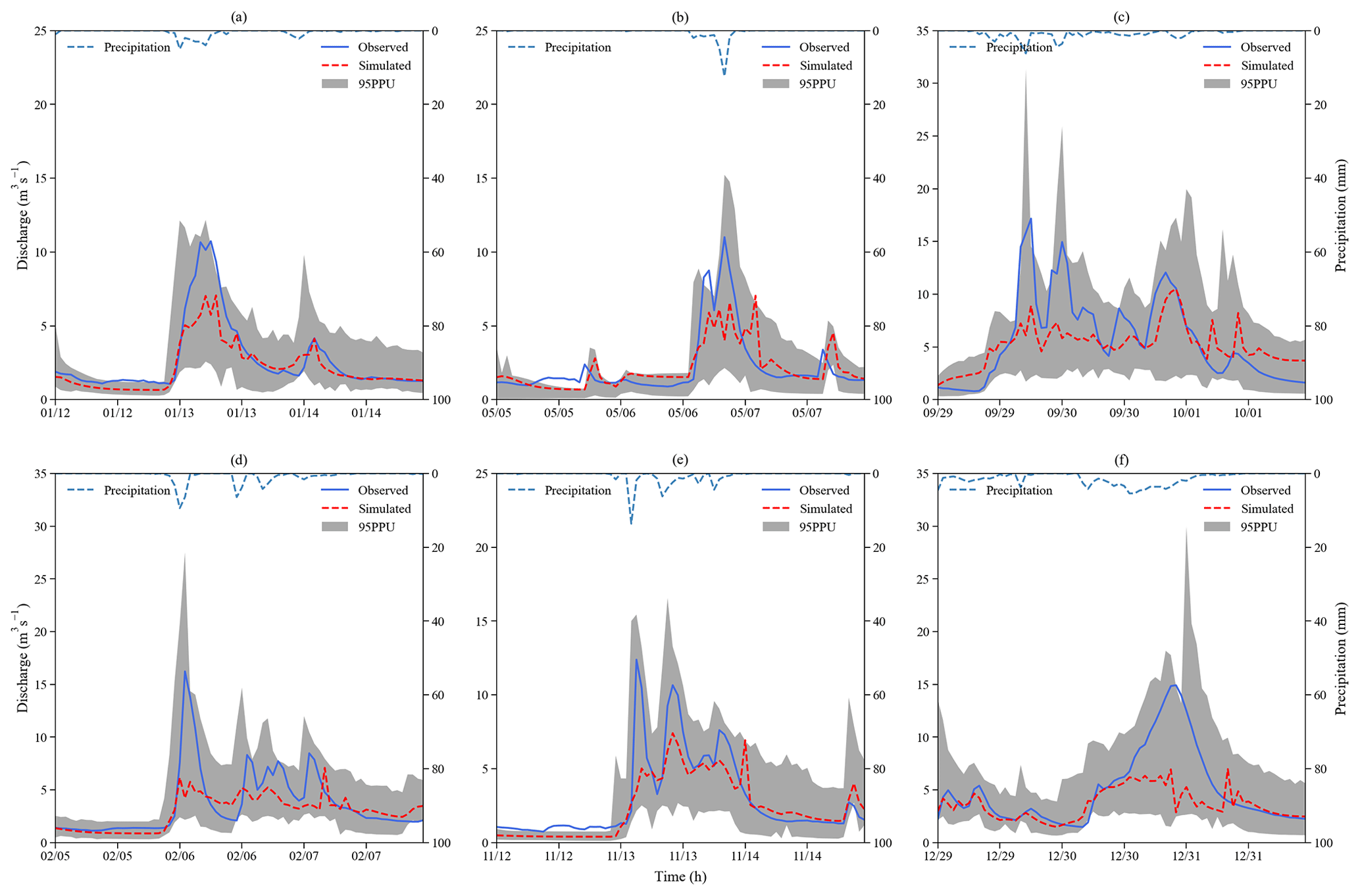
Figure 4Observed and simulated hourly discharge (m3 s−1) using the GAML method for the heavy rainfall events that occurred in 2018 and 2019. (a) Event from 12–14 January 2018. (b) Event from 5–7 May 2018. (c) Event from 29 September–1 October 2018. (d) Event from 5–7 February 2019. (e) Event from 12–14 November 2019. (f) Event from 29–31 December 2019.
3.3 Comparison of selected rainfall events
Figure 4 shows the hydrographs of selected high-rainfall events that occurred in the years 2018 and 2019 (Tatoi station; Lagouvardos et al., 2017). According to the study area's intensity–duration–frequency (IDF) curves, the approximate return period of the selected episodes was 10 years (T = 10 years). These events were investigated to examine the accuracy of the subdaily model and to compare the peak discharges and time of the peak of the two models. Table 6 displays the rainfall characteristics of each event (i.e., peak discharge, time of peak, and average discharge).
Table 6Rainfall characteristics of selected events for the years 2018 and 2019.

Generally, the hourly model underestimated the peak flows with values much lower than the observations for the majority of the events. These results confirm that the daily model using the CN method estimated the observed values better than the hourly model using the GAML method and was able to estimate, with greater accuracy, the peak discharge in most of the events. In addition, Fig. 4a–c show that the discharge simulation improved after the main peak discharge event, especially in the last peaks. The improvement in the simulation as the rainfall events progressed indicates that the simulation requires time to adapt to the hydrological processes and conditions of the catchment (e.g., antecedent soil moisture conditions). These outcomes are similar to those of previous studies, which concluded that the best subdaily performance for streamflow simulation appeared in wet antecedent soil moisture conditions and suggested that the GAML method needs to improve the equation for the infiltration routine (Jeong et al., 2010; Kannan et al., 2007; Meaurio et al., 2021).
The better performance of the CN method compared to the GAML method in this study is consistent with the results of other studies (Bauwe et al., 2016; Ficklin and Zhang, 2013; Kannan et al., 2007; King et al., 1999). Bauwe et al. (2016) evaluated both CN and GAML methods and highlighted that the CN method performed slightly better than the GAML method. Ficklin and Zhang (2013) generally suggested that, for daily simulations, the CN method predicted streamflow more accurately than the GAML model. Kannan et al. (2007) identified a suitable combination of ET runoff-generation methods and reported that the CN method performed better than the GAML method. Kannan et al. (2007) conducted a sensitivity analysis to identify the best combination of evapotranspiration and runoff method for hydrological modeling and concluded that the CN method performed better than the GAML method for streamflow because the GAML method tends to hold more water in the soil profile and predict a lower peak runoff rate. King et al. (1999) concluded that the GAML method appeared to have more limitations in accounting for seasonal variability than the CN method.
Hydrological calibration includes uncertainties due to conceptual simplification, processes not incorporated in the model, and unknown processes to the modeler which interfere with the natural behavior of the system (Abbaspour et al., 2015). In this study, the sources of uncertainty can be explained by the following:
- i.
The characteristics of an urban/peri-urban catchment. The study area is a hybrid landscape in which urban and rural characteristics coexist and interact. The different and changing land uses create a complex system with high variability in management practices and diverse hydrological processes (Becker et al., 2019). Furthermore, these systems are characterized by human-made interventions (e.g., unidentified discharges, agricultural activities, and dumping of construction materials), which are not well known to the modeler and can increase uncertainty (Immerzeel and Droogers, 2008).
- ii.
The inaccuracies in the quality of input and observed data. The interaction between the urban environment and agricultural activities may not be captured by the resolution of the soil and land use maps. This could increase the difficulty for the SWAT model to represent the actual conditions of the study area and further affect the results. The spatial variability in precipitation and discharge were not also captured accurately by the monitoring stations of the study area, which could have contributed to the simulation uncertainty. In addition, inaccuracies in the estimation of channel and hillslope velocities and channel geometry, in the nature of the sensor, environmental conditions, and data collection can generate variability, lead to undesired trends, and influence the model results (Guzman et al., 2015; Kamali et al., 2017).
- iii.
The differences behind the mechanisms of the CN method and the GAML method for surface runoff estimation. In this study, the daily model produced higher discharge peaks than the hourly model and generally estimated better the observed values. These results could be explained by the disadvantages of the GAML method. The CN method requires minimum land use, soil, elevation, and daily rainfall data as input. On the other hand, the GAML method requires detailed soil information and high-resolution rainfall data in a subdaily time step as input, which can be challenging and difficult to obtain (King et al., 1999). The GAML method also assumes that the soil profile is characterized by homogeneity and that the previous soil moisture is distributed uniformly in the soil profile (Jeong et al., 2010). In addition, according to the GAML method, when the precipitation rate is less than the infiltration rate, all precipitation will infiltrate the soil profile (Ficklin and Zhang, 2013; King et al., 1999). Figure 2 reflects the assumption of the GAML method that surface runoff is estimated only when the precipitation rate is greater than the infiltration rate. Hence, the uncertainty in the resolution of the rainfall data, the heterogeneity of the soil formations, the size of the catchment, and the upcoming difficulty in determining the parameters' values for parameterization could affect the method's efficiency (Jeong et al., 2010). The selection of the subdaily precipitation input time step and the resolution of the precipitation data have a significant impact on model results when using the GAML method, and it should be based on the scale and characteristics of the watershed (Bauwe et al., 2016; Kannan et al., 2007).
- iv.
The conceptual simplifications made during the model parameterization process. The initial ranges of the calibrating parameters were set according to the literature and sensitivity analysis. Then, based on the performance of the default model, specific parameters were parameterized using calibration protocols (Abbaspour et al., 2015). The ranges of the calibrating parameters should be kept within reasonable limits, using quantitative statistics and graphical comparisons to ensure that hydrological processes represent the characteristic of the study area (Daggupati et al., 2015b). The choice of the objective function and the selection of the values of the parameters that influence surface runoff, groundwater, channel routing, and evapotranspiration is a critical point in model calibration, which can increase the uncertainty in the results (Polanco et al., 2017).
Experimental catchments provide long-term time series of hydrological data, which are essential for improved application of best management practices and the development and validation of watershed models. In this study, discharge was monitored for 3 years (2017–2019) in an experimental basin with mixed-land-use characteristics (i.e., urban/peri-urban) in Athens, Greece. Discharge simulation, calibration, and validation were achieved with the SWAT model, which has been increasingly used to support decisions on various environmental issues and policy directions. Daily and hourly rainfall observations were used as inputs to investigate the influence of the rainfall resolution on model performance in order to analyze the mechanisms governing surface runoff at the catchment scale. Surface runoff was estimated using the CN method for the daily model and the GAML method for the hourly model.
A sensitivity analysis conducted in this study showed that the parameters related to groundwater flow were more sensitive for daily time intervals, and channel-routing parameters were more influential for hourly time intervals. These findings indicate that the model operational time step affects the parameters' sensitivity to the model output, thus demonstrating the need for a different model strategy for the simulation of subdaily hydrological processes.
Quantitative statistics of the observed and the simulated records indicate that the calibration and validation processes produced acceptable results for both runoff estimation methods. Additionally, graphical techniques at the outlet station show that both models succeed in capturing the majority of the seasonality and peak discharge. Generally, the daily model performed better than the subdaily model in simulating runoff. The CN method produced higher discharge peaks than the GAML method and estimated the observed values better. In particular, from the comparison of the selected rainfall events, the critical role of the antecedent soil moisture conditions of the catchment and their impact on subdaily performance is also evident, indicating the need for the improvement of the SWAT subdaily option for soil moisture estimation. The differences in the calibrated values of the two models lay mostly in the different runoff estimation methods used by the two models. In addition, errors in the quality of input data, diverse management practices and hydrological processes of an urban/peri-urban environment, unknown processes to the modeler, and conceptual simplifications made during the model structure/calibration process may increase the uncertainty in the outputs.
Overall, the general agreement between observations and simulations in both models suggests that the SWAT model appears to be a reliable tool for predicting discharge in a mixed-land-use basin with a high complexity and spatial distribution of input data. This study contributed to understanding the mechanisms controlling surface runoff and the parameters that influence the hydrological processes that take place in an urban/peri-urban hydrological environment. Furthermore, the results of this study could help planners and managers to decide which time step is more useful regarding their goals and will provide a calibrated tool to assess potential hydrological impacts of future planning and development activities. However, it should be noted that several factors such as data limitation, observational errors in input data, spatiotemporal-scale complexities, and inaccuracies in model structure may lead to uncertainty in model outputs. In the future, emphasis will be placed on the investigation of a correlation between the antecedent moisture conditions and hourly model performance when more data become available and on quantifying the parameter uncertainty by including more observed variables in the calibration process, such as evapotranspiration and soil moisture satellite data.
The SWAT model was used for the discharge simulation and is available at https://doi.org/10.1111/j.1752-1688.1998.tb05961.x (Arnold et al., 1998). The digital elevation model (DEM) data were downloaded from https://earthexplorer.usgs.gov/ (U.S. Geological Survey, 2020). The land use data were downloaded from https://land.copernicus.eu/ (Corine Land Cover, 2018). The soil data were downloaded from http://www.fao.org/ (FAO et al., 2012). The weather data were downloaded from https://www.meteo.gr/ (Lagouvardos et al., 2017; National Observatory of Athens, 2020). The discharge data were downloaded from https://openhi.net/ (Mamassis et al., 2021; Open Hydrosystem Information Network, 2020).
EK performed the simulations, analyzed the results, and prepared the paper, with contributions from all co-authors. NM and AK contributed to the conception and methodology of this study. AK was the supervisor of the research project and sourced the funding that led to this publication.
The contact author has declared that none of the authors has any competing interests.
Publisher's note: Copernicus Publications remains neutral with regard to jurisdictional claims in published maps and institutional affiliations.
This research is part of the project “UPWATER: Understanding groundwater Pollution to protect and enhance WATER quality” (grant no. 101081807). The authors are grateful to Nancy Sammons, Information Technology Specialist of the SWAT team, and Chris George, Software Engineer of the SWAT team, for their help with the SWAT software.
This research has been funded by the European Union under the project “UPWATER: Understanding groundwater Pollution to protect and enhance WATER quality” within Horizon Europe work programme (grant no. 101081807).
This paper was edited by Nunzio Romano and reviewed by five anonymous referees.
Abbaspour, K. C., Johnson, C. A., and van Genuchten, M. T.: Estimating Uncertain Flow and Transport Parameters Using a Sequential Uncertainty Fitting Procedure, Vadose Zone J., 3, 1340–1352, https://doi.org/10.2113/3.4.1340, 2004.
Abbaspour, K. C., Yang, J., Maximov, I., Siber, R., Bogner, K., Mieleitner, J., Zobrist, J., and Srinivasan, R.: Modelling hydrology and water quality in the pre-alpine/alpine Thur watershed using SWAT, J. Hydrol., 333, 413–430, https://doi.org/10.1016/j.jhydrol.2006.09.014, 2007.
Abbaspour, K. C., Rouholahnejad, E., Vaghefi, S., Srinivasan, R., Yang, H., and Kløve, B.: A continental-scale hydrology and water quality model for Europe: Calibration and uncertainty of a high-resolution large-scale SWAT model, J. Hydrol., 524, 733–752, https://doi.org/10.1016/j.jhydrol.2015.03.027, 2015.
Arnold, J. G., Srinivasan, R., Muttiah, R. S., and Williams, J. R.: Large Area Hydrologic Modeling and Assessment Part I: Model Development, J. Am. Water Resour. As., 34, 73–89, https://doi.org/10.1111/j.1752-1688.1998.tb05961.x, 1998.
Arnold, J. G., Moriasi, D. N., Gassman, P. W., Abbaspour, K. C., White, M. J., Srinivasan, R., Santhi, C., Harmel, R. D., Van Griensven, A., Van Liew, M. W., Kannan, N., and Jha, M. K.: SWAT: Model Use, Calibration, and Validation, T. ASABE, 55, 1491–1508, https://doi.org/10.13031/2013.42256, 2012.
Arnold, J. G., Youssef, M. A., Yen, H., White, M. J., Sheshukov, A. Y., Sadeghi, A. M., Moriasi, D. N., Steiner, J. L., Amatya, D. M., Skaggs, R. W., Haney, E. B., Jeong, J., Arabi, M., and Gowda, P. H.: Hydrological Processes and Model Representation: Impact of Soft Data on Calibration, T. ASABE, 58, 1637–1660, https://doi.org/10.13031/trans.58.10726, 2015.
Bauwe, A., Kahle, P., and Lennartz, B.: Hydrologic evaluation of the curve number and Green and Ampt infiltration methods by applying Hooghoudt and Kirkham tile drain equations using SWAT, J. Hydrol., 537, 311–321, https://doi.org/10.1016/j.jhydrol.2016.03.054, 2016.
Bauwe, A., Tiedemann, S., Kahle, P., and Lennartz, B.: Does the Temporal Resolution of Precipitation Input Influence the Simulated Hydrological Components Employing the SWAT Model?, J. Am. Water Resour. As., 53, 997–1007, https://doi.org/10.1111/1752-1688.12560, 2017.
Becker, R., Koppa, A., Schulz, S., Usman, M., aus der Beek, T., and Schüth, C.: Spatially distributed model calibration of a highly managed hydrological system using remote sensing-derived ET data, J. Hydrol., 577, 123944, https://doi.org/10.1016/j.jhydrol.2019.123944, 2019.
Bogena, H. R., White, T., Bour, O., Li, X., and Jensen, K. H.: Toward Better Understanding of Terrestrial Processes through Long-Term Hydrological Observatories, Vadose Zone J., 17, 180194, https://doi.org/10.2136/vzj2018.10.0194, 2018.
Boithias, L., Sauvage, S., Lenica, A., Roux, H., Abbaspour, K., Larnier, K., Dartus, D., and Sánchez-Pérez, J.: Simulating Flash Floods at Hourly Time-Step Using the SWAT Model, Water, 9, 929, https://doi.org/10.3390/w9120929, 2017.
Brighenti, T. M., Bonumá, N. B., Srinivasan, R., and Chaffe, P. L. B.: Simulating sub-daily hydrological process with SWAT: a review, Hydrolog. Sci. J., 64, 1415–1423, https://doi.org/10.1080/02626667.2019.1642477, 2019.
Campbell, A., Pradhanang, S. M., Kouhi Anbaran, S., Sargent, J., Palmer, Z., and Audette, M.: Assessing the impact of urbanization on flood risk and severity for the Pawtuxet watershed, Rhode Island, Lake Reserv. Manage., 34, 74–87, https://doi.org/10.1080/10402381.2017.1390016, 2018.
Cheng, Q. B., Reinhardt-Imjela, C., Chen, X., Schulte, A., Ji, X., and Li, F. L.: Improvement and comparison of the rainfall–runoff methods in SWAT at the monsoonal watershed of Baocun, Eastern China, Hydrolog. Sci. J., 61, 1460–1476, https://doi.org/10.1080/02626667.2015.1051485, 2016.
CORINE Land Cover (CLC): Land use data, https://land.copernicus.eu/ (last access: 15 December 2020), 2018.
Daggupati, P., Yen, H., White, M. J., Srinivasan, R., Arnold, J. G., Keitzer, C. S., and Sowa, S. P.: Impact of model development, calibration and validation decisions on hydrological simulations in West Lake Erie Basin, Hydrol. Process., 29, 5307–5320, https://doi.org/10.1002/hyp.10536, 2015a.
Daggupati, P., Yen, H., White, M. J., Srinivasan, R., Arnold, J. G., Keitzer, C. S., and Sowa, S. P.: Impact of model development, calibration and validation decisions on hydrological simulations in West Lake Erie Basin, Hydrol. Process., 29, 5307–5320, https://doi.org/10.1002/hyp.10536, 2015b.
Dile, Y. T., Daggupati, P., George, C., Srinivasan, R., and Arnold, J.: Introducing a new open source GIS user interface for the SWAT model, Environ. Modell. Softw., 85, 129–138, https://doi.org/10.1016/j.envsoft.2016.08.004, 2016.
Douglas-Mankin, K. R., Srinivasan, R., and Arnold, J. G.: Soil and Water Assessment Tool (SWAT) Model: Current Developments and Applications, T. ASABE, 53, 1423–1431, https://doi.org/10.13031/2013.34915, 2010.
Engel, B., Storm, D., White, M., Arnold, J., and Arabi, M.: A Hydrologic/Water Quality Model Applicati1, J. Am. Water Resour. As., 43, 1223–1236, https://doi.org/10.1111/j.1752-1688.2007.00105.x, 2007.
FAO, IIASA, ISRIC and ISSCAS: Harmonized World Soil Database Version 1.2, Food & Agriculture Organization of the UN, Rome, Italy, and International Institute for Applied Systems Analysis, Laxenburg, Austria, http://www.fao.org/ (last access: 10 December 2020), 2012.
Ficklin, D. L. and Zhang, M.: A Comparison of the Curve Number and Green-Ampt Models in an Agricultural Watershed, T. ASABE, 56, 61–69, https://doi.org/10.13031/2013.42590, 2013.
Gassman, P. W., Reyes, M. R., Green, C. H., and Arnold, J. G.: The Soil and Water Assessment Tool: Historical Development, Applications, and Future Research Directions, T. ASABE, 50, 1211–1250, https://doi.org/10.13031/2013.23637, 2007.
Gassman, P. W., Sadeghi, A. M., and Srinivasan, R.: Applications of the SWAT Model Special Section: Overview and Insights, J. Environ. Qual., 43, 1–8, https://doi.org/10.2134/jeq2013.11.0466, 2014.
Golmohammadi, G., Rudra, R., Dickinson, T., Goel, P., and Veliz, M.: Predicting the temporal variation of flow contributing areas using SWAT, J. Hydrol., 547, 375–386, https://doi.org/10.1016/j.jhydrol.2017.02.008, 2017.
Goodrich, D. C., Heilman, P., Anderson, M., Baffaut, C., Bonta, J., Bosch, D., Bryant, R., Cosh, M., Endale, D., Veith, T. L., Havens, S. C., Hedrick, A., Kleinman, P. J., Langendoen, E. J., McCarty, G., Moorman, T., Marks, D., Pierson, F., Rigby, J. R., Schomberg, H., Starks, P., Steiner, J., Strickland, T., and Tsegaye, T.: The USDA-ARS Experimental Watershed Network: Evolution, Lessons Learned, Societal Benefits, and Moving Forward, Water Resour. Res., 57, 0–3, https://doi.org/10.1029/2019WR026473, 2020.
Gupta, H. V., Sorooshian, S., and Yapo, P. O.: Status of Automatic Calibration for Hydrologic Models: Comparison with Multilevel Expert Calibration, J. Hydrol. Eng., 4, 135–143, https://doi.org/10.1061/(ASCE)1084-0699(1999)4:2(135), 1999.
Guzman, J. A., Shirmohammadi, A., Sadeghi, A. M., Wang, X., Chu, M. L., Jha, M. K., Parajuli, P. B., Harmel, R. D., Khare, Y. P., and Hernandez, J. E.: Uncertainty considerations in calibration and validation of hydrologic and water quality models, T. ASABE, 58, 1745–1762, https://doi.org/10.13031/trans.58.10710, 2015.
Han, E., Merwade, V., and Heathman, G. C.: Implementation of surface soil moisture data assimilation with watershed scale distributed hydrological model, J. Hydrol., 416–417, 98–117, https://doi.org/10.1016/j.jhydrol.2011.11.039, 2012.
Harmel, R. D., Smith, P. K., Migliaccio, K. W., Chaubey, I., Douglas-Mankin, K. R., Benham, B., Shukla, S., Muñoz-Carpena, R., and Robson, B. J.: Evaluating, interpreting, and communicating performance of hydrologic/water quality models considering intended use: A review and recommendations, Environ. Modell. Softw., 21, 40–51, 2014.
Hrachowitz, M., Benettin, P., van Breukelen, B. M., Fovet, O., Howden, N. J. K., Ruiz, L., van der Velde, Y., and Wade, A. J.: Transit times-the link between hydrology and water quality at the catchment scale, WIREs Water, 3, 629–657, https://doi.org/10.1002/wat2.1155, 2016.
Immerzeel, W. W. and Droogers, P.: Calibration of a distributed hydrological model based on satellite evapotranspiration, J. Hydrol., 349, 411–424, https://doi.org/10.1016/j.jhydrol.2007.11.017, 2008.
Jeong, J., Kannan, N., Arnold, J., Glick, R., Gosselink, L., and Srinivasan, R.: Development and Integration of Sub-hourly Rainfall-Runoff Modeling Capability Within a Watershed Model, Water Resour. Manag., 24, 4505–4527, https://doi.org/10.1007/s11269-010-9670-4, 2010.
Kamali, B., Abbaspour, K. C., and Yang, H.: Assessing the uncertainty of multiple input datasets in the prediction of water resource components, Water (Switzerland), 9, 709, https://doi.org/10.3390/w9090709, 2017.
Kannan, N., White, S. M., Worrall, F., and Whelan, M. J.: Sensitivity analysis and identification of the best evapotranspiration and runoff options for hydrological modelling in SWAT-2000, J. Hydrol., 332, 456–466, https://doi.org/10.1016/j.jhydrol.2006.08.001, 2007.
King, K. W., Arnold, J. G., and Bingner, R. L.: Comparison of Green-Ampt and curve number methods on Goodwin Creek Watershed using SWAT, Transactions of the American Society of Agricultural Engineers, 42, 919–925, https://doi.org/10.13031/2013.13272, 1999.
Lagouvardos, K., Kotroni, V., Bezes, A., Koletsis, I., Kopania, T., Lykoudis, S., Mazarakis, N., Papagiannaki, K., and Vougioukas, S.: The automatic weather stations NOANN network of the National Observatory of Athens: operation and database, Geosci. Data J., 4, 4–16, https://doi.org/10.1002/gdj3.44, 2017.
Li, Y. and DeLiberty, T.: Evaluating hourly SWAT streamflow simulations for urbanized and forest watersheds across northwestern Delaware, US, Stoch. Env. Res. Risk A., 35, 1145–1159, https://doi.org/10.1007/s00477-020-01904-y, 2020.
Maharjan, G. R., Park, Y. S., Kim, N. W., Shin, D. S., Choi, J. W., Hyun, G. W., Jeon, J. H., Ok, Y. S., and Lim, K. J.: Evaluation of SWAT sub-daily runoff estimation at small agricultural watershed in Korea, Frontiers of Environmental Science and Engineering in China, 7, 109–119, https://doi.org/10.1007/s11783-012-0418-7, 2013.
Mamassis, N., Mazi, K., Dimitriou, E., Kalogeras, D., Malamos, N., Lykoudis, S., Koukouvinos, A., Tsirogiannis, I., Papageorgaki, I., Papadopoulos, A., Panagopoulos, Y., Koutsoyiannis, D., Christofides, A., Efstratiadis, A., Vitantzakis, G., Kappos, N., Katsanos, D., Psiloglou, B., Rozos, E., Kopania, T., Koletsis, I., and Koussis, A.: OpenHi.net: A Synergistically Built, National-Scale Infrastructure for Monitoring the Surface Waters of Greece, Water, 13, 2779, https://doi.org/10.3390/w13192779, 2021.
Meaurio, M., Zabaleta, A., Srinivasan, R., Sauvage, S., Sánchez-Pérez, J.-M., Lechuga-Crespo, J. L., and Antiguedad, I.: Long-term and event-scale sub-daily streamflow and sediment simulation in a small forested catchment, Hydrolog. Sci. J., 66, 862–873, https://doi.org/10.1080/02626667.2021.1883620, 2021.
Mein, R. G. and Larson, C. L.: Modeling Infiltration during a Steady Rain, Water Resour. Res., 9, 384–394, 1973.
Moriasi, D. N., Arnold, J. G., Van Liew, M. W., Bingner, R. L., Harmel, R. D., and Veith, T. L.: Model Evaluation Guidelines for Systematic Quantification of Accuracy in Watershed Simulations, T. ASABE, 50, 885–900, https://doi.org/10.13031/2013.23153, 2007.
Moriasi, D. N., Gitau, M. W., Pai, N., and Daggupati, P.: Hydrologic and water quality models: Performance measures and evaluation criteria, T. ASABE, 58, 1763–1785, https://doi.org/10.13031/trans.58.10715, 2015.
Nash, J. E. and Sutcliffe, J. V.: River flow forecasting through conceptual models part I - A discussion of principles, J. Hydrol., 10, 282–290, https://doi.org/10.1016/0022-1694(70)90255-6, 1970.
National Observatory of Athens (NOA): Weather data, National Observatory of Athens (NOA) [data set], https://www.meteo.gr/, last access: 10 December 2020.
Neitsch, S. L., Arnold, J. G., Kiniry, J. R., and Williams, J. R.: Soil & Water Assessment Tool Theoretical Documentation Version 2009, Texas Water Resources Institute Technical Report No. 406, Texas A & M University System, Texas, USA, https://hdl.handle.net/1969.1/128050 (last access: 5 December 2020), 2011.
Open Hydrosystem Information Network (OpenHi.net): Observed streamflow data, https://openhi.net/, last access: 20 December 2020.
Polanco, E. I., Fleifle, A., Ludwig, R., and Disse, M.: Improving SWAT model performance in the upper Blue Nile Basin using meteorological data integration and subcatchment discretization, Hydrol. Earth Syst. Sci., 21, 4907–4926, https://doi.org/10.5194/hess-21-4907-2017, 2017.
Soil Conservation Service, S.: National Engineering Handbook, Section 4, Hydrology, Department of Agriculture, Washington, DC, USA, 1972.
Stockinger, M. P., Bogena, H. R., Lücke, A., Diekkrüger, B., Cornelissen, T., and Vereecken, H.: Tracer sampling frequency influences estimates of young water fraction and streamwater transit time distribution, J. Hydrol., 541, 952–964, https://doi.org/10.1016/j.jhydrol.2016.08.007, 2016.
Tan, M. L., Gassman, P. W., Yang, X., and Haywood, J.: A review of SWAT applications, performance and future needs for simulation of hydro-climatic extremes, Adv. Water Resour., 143, 103662, https://doi.org/10.1016/j.advwatres.2020.103662, 2020.
Tauro, F., Selker, J., van de Giesen, N., Abrate, T., Uijlenhoet, R., Porfiri, M., Manfreda, S., Caylor, K., Moramarco, T., Benveniste, J., Ciraolo, G., Estes, L., Domeneghetti, A., Perks, M. T., Corbari, C., Rabiei, E., Ravazzani, G., Bogena, H., Harfouche, A., Brocca, L., Maltese, A., Wickert, A., Tarpanelli, A., Good, S., Lopez Alcala, J. M., Petroselli, A., Cudennec, C., Blume, T., Hut, R., and Grimaldi, S.: Measurements and Observations in the XXI century (MOXXI): innovation and multi-disciplinarity to sense the hydrological cycle, Hydrolog. Sci. J., 63, 169–196, https://doi.org/10.1080/02626667.2017.1420191, 2018.
U.S. Geological Survey (USGS): Shuttle Radar Topography Mission (SRTM) Global, DEM data, Open Topography, U.S. Geological Survey (USGS) [data set], https://earthexplorer.usgs.gov/, last access: 5 December 2020.
Yang, X., Liu, Q., He, Y., Luo, X., and Zhang, X.: Comparison of daily and sub-daily SWAT models for daily streamflow simulation in the Upper Huai River Basin of China, Stoch. Env. Res. Risk A., 30, 959–972, https://doi.org/10.1007/s00477-015-1099-0, 2016.
Yu, D., Xie, P., Dong, X., Hu, X., Liu, J., Li, Y., Peng, T., Ma, H., Wang, K., and Xu, S.: Improvement of the SWAT model for event-based flood simulation on a sub-daily timescale, Hydrol. Earth Syst. Sci., 22, 5001–5019, https://doi.org/10.5194/hess-22-5001-2018, 2018.