the Creative Commons Attribution 4.0 License.
the Creative Commons Attribution 4.0 License.
 | 14 Feb 2023
Evidence-based requirements for perceptualising intercatchment groundwater flow in hydrological models
Louisa D. Oldham
Jim Freer
Gemma Coxon
Nicholas Howden
John P. Bloomfield
Christopher Jackson
Groundwater-dominated catchments are often critical for nationally important water resources. Many conceptual rainfall–runoff models tend to degrade in their model performance in groundwater-dominated catchments, as they are rarely designed to simulate spatial groundwater behaviours or interactions with surface waters. Intercatchment groundwater flow is one such neglected variable. Efforts have been made to incorporate this process into existing models, but there is a need for improving our perceptual models of groundwater–surface water interactions prior to any model modifications.
In this study, national meteorological, hydrological, hydrogeological, geological and artificial influence (characterising abstractions and return flows) datasets are used to infer a perceptual model of intercatchment groundwater flow (IGF) and how it varies across the river Thames, United Kingdom (UK). We characterise the water balance, presence of gaining/losing river reaches and intra-annual dynamics in 80 subcatchments of the river Thames, taking advantage of its wealth of data, densely gauged river network and geological variability.
We show the prevalence of non-conservative river reaches across the study area, with heterogeneity both between, and within, geological units, giving rise to a complex distribution of recharge and discharge points along the river network. We infer where non-conservative reaches can be attributed to IGF and where other processes (e.g. surface water abstractions) are the likely cause. Through analysis of recorded reach length water balance data and hydrogeological perceptualisation, we conclude that outcrops of carbonate fractured aquifers (Chalk and Jurassic limestone) show evidence of IGF both from headwater to downstream reaches, and out-of-catchment via spring lines. We found variability across the study area, with more seasonality and variability in river catchments on Jurassic limestone outcrops compared to Chalk and Lower Greensand outcrops. Our results demonstrate the need for local investigation and hydrogeological perceptualisation within regional analysis, which we show to be achievable given relatively simple geological interpretation and data requirements. We support the inclusion of IGF fluxes within existing models to enable calibration improvements in groundwater-dominated catchments, but with geologically specific characteristics, and (when perceptually appropriate) connectivity between catchments.
- Article
(3605 KB) - Full-text XML
-
Supplement
(991 KB) - BibTeX
- EndNote


Groundwater-dominated river catchments are often critical for nationally important water resources (Yang et al., 2017), with groundwater itself accounting for, on average, one-third of global human water consumption (IGRAC, 2020). However, conceptual rainfall–runoff models used for the simulation of catchment river flows are rarely designed to simulate spatial groundwater behaviours or interactions with surface waters (Wanders et al., 2011). Many conceptual catchment models applied to groundwater-dominated catchments tend to degrade in their model performance metrics when simulating observed river flow (Le Moine et al., 2005; Pellicer-Martinez et al., 2015; McMillan et al., 2016; Coxon et al., 2019; Lane et al., 2019), having to resort to the selection of unrealistic parameters (Goswami and O'Connor, 2010) or factoring of climate inputs or catchment area (Le Moine et al., 2007) to achieve acceptable calibration results. To enable improvements of conceptual models to address this lack of groundwater process representation, groundwater and surface water processes need to be holistically reviewed and conceptualised (Barthel and Banzhaf, 2016).
1.1 Intercatchment groundwater flow
Under the Tothian framework of groundwater flow, local, intermediate and regional groundwater systems can be present contemporaneously (Toth, 1963). At the subcatchment scale and under natural conditions, surface water boundaries are topographical, whilst groundwater boundaries are a complex manifestation of topographic lows, the spatial distribution of recharge, and subsurface hydraulic properties that depend on lithology. Under the appropriate geological conditions, there is, therefore, the potential for precipitation falling in one surface water catchment to flow to an adjacent surface water catchment's streamflow channel via the groundwater flow system (intercatchment groundwater flow (IGF)), across the topographical surface water divide and bypassing the “donor” stream's outlet gauge (Le Moine et al., 2005; Gascoin et al., 2009; Pellicer-Martinez and Martinez-Paz, 2014; Barthel and Banzhaf, 2016; Bouaziz et al., 2018; Fan, 2019; Le Mesnil et al., 2020). IGF can result in a net loss or gain to a surface water catchment (termed a “non-conservative” catchment) and can be an important term in a catchment's water balance as both unmeasured, and often unaccounted for, inflow and outflow (Yeh et al., 1998; Bouaziz et al., 2018; Fan, 2019; Le Mesnil et al., 2020; Wagener et al., 2021). Yet the impact of IGF on catchments' water balances is an often neglected variable in conceptual hydrological modelling (Pellicer-Martinez and Martinez-Paz, 2014).
Studies have found IGF to be most prominent in headwater catchments (Bouaziz et al., 2018; Fan, 2019) of increasing slope (Ameli et al., 2018), underlain by high-permeability aquifers (Le Moine et al., 2005; Schaller and Fan, 2009) and in drier climates (Schaller and Fan, 2009), but with geological spatial variability being the key control on the prevalence of IGF (Genereux et al., 2002; Schaller and Fan, 2009; Frisbee et al., 2016; Bouaziz et al., 2018; Le Mesnil et al., 2020). Correlations to IGF presence and magnitude have also been made to larger basin sizes (Schaller and Fan, 2009; Bouaziz et al., 2018), although this itself is an anthropogenic variable as it is dependent on the human placement of river gauging stations with often no consideration of underlying hydrogeological flowpaths (Krabbenhoft et al., 2022). Water balance analysis (e.g. Schaller and Fan, 2009; Bouaziz et al., 2018), geochemical analysis (e.g. Genereux et al., 2002; Frisbee et al., 2016), geomorphic analysis (e.g. Frisbee et al., 2016) and modelling methods (e.g. Zanon et al., 2014; Bouaziz et al., 2018) have been used to spatially characterise and quantify IGF. The prevalence of intra-annual temporal variation in IGF has also been shown (Bouaziz et al., 2018). These studies have all emphasised the need for local-scale geological interpretation in the understanding of this complex physical process (Fan, 2019).
1.2 Efforts to address the “watertight substratum” challenge
In conceptual hydrological catchment models, groundwater tends to be represented via a secondary, deeper subsurface water store, with fluxes representing groundwater contribution from the saturated zone to river flows controlled by a baseflow parameter. Lumped conceptual models often calculate only one head of groundwater for an entire catchment (Wanders et al., 2011). A closed water balance is routinely ensured, where a surface water catchment is set up assuming topographical controls, underlain by a low permeability horizontal substratum and its fluxes self-contained (Pellicer-Martinez and Martinez-Paz, 2014; Barthel and Banzhaf, 2016) – termed the “watertight substratum” approach (Le Moine et al., 2005).
A parameterised “loss function” has been incorporated by hydrologists into a number of conceptual rainfall–runoff models such as PMS (Pellicer-Martinez et al., 2015), abcd (Pellicer-Martinez and Martinez-Paz, 2014), GR4J (Le Moine et al., 2005, 2007), SMAR (Goswami and O'Connor, 2010), HYPE (Lindstrom et al., 2010) and TopNet-GW (Yang et al., 2017). These flux functions can generate a permanent loss to the system in lumped models (e.g. GR4J, Le Moine et al., 2005) and improve calibrations in groundwater-dominated catchments. However, owing to an absence of connectivity between subcatchments' deep groundwater stores, they do not represent the physical reality of IGF. In a semi-distributed hydrological modelling framework, IGF between catchments can be modelled via predefined network linkages (e.g. abcd, Pellicer-Martinez and Martinez-Paz, 2014) and temporal variability can be applied (e.g. TopNet-GW, Yang et al., 2017). However, a priori perceptualisation of IGF spatial and temporal variability by hydrologists has been to date solely based on observed accretion flow profiling (Yang et al., 2017) or loss/gain water balance output from a lumped catchment model (Pellicer-Martinez and Martinez-Paz, 2014), rather than hydrogeological perceptualisation.
1.3 Holistic surface water–groundwater perceptualisation
While the loss function approaches have improved model performance for surface hydrological predictions and incorporated a key “missing” hydrological variable, the inclusion of these IGF losses in conceptual rainfall–runoff models seems to be rarely evaluated as to its realism and whether spatial patterns of losses relate to understanding of the geological controls in and between catchments and river reaches. Editing groundwater processes within a model without a preceding perceptualisation of the groundwater environment can be detrimental to model performance and lead to results at odds with the physical characteristics of a catchment (Hughes et al., 2015). Perceptualisation is the development of a perceptual model, whereby a system is described qualitatively (and, potentially, quantitatively) and is akin to a hydrogeologist's conceptual model (Wagener et al., 2021). (The term “perceptual” is used by hydrologists in place of “conceptual” to avoid confusion with the type of hydrological mathematical model). Perceptual models are routinely developed by hydrogeologists (Wagener et al., 2021) prior to groundwater modelling (e.g. Entec UK Ltd., 2008; Environment Agency, 2010; ESI Ltd., 2013).
We believe that there is a need for greater emphasis on improving our holistic groundwater–surface water perceptualisations of surface water catchments, prior to any hydrological conceptual model edits. This would allow the modeller to make informed decisions and reduce the risk of a model edit being used as a proxy for input data errors or parameterisation limitations (Goswami and O'Connor, 2010; Lane et al., 2019), whilst linking groundwater–surface water interaction theory back into hydrological analysis, as advocated by Fan (2019). This can be a challenging task as the scale of groundwater influences can be mismatched to the local hydrology and hydrogeological evidence available and can involve complex lithologies. A “high-level” hydrogeological analysis is here advocated, focussed on the needs of the surface water catchment modeller.
This paper presents a high-level perceptualisation of inferred IGF for the purposes of rationalising the spatial development of catchment-based hydrological conceptual modelling. Quantifying the water balance using available national meteorological, hydrological, hydrogeological, geological and human influences datasets enabled us to develop a perceptual model of IGF, where we have identified the location and direction of IGF at a high level. Our perceptual model does not quantify the detailed specifics and directions of IGF, owing to the underlying information and analyses we have available. However, we can identify river reach lengths that have anomalous water balances that infer IGF processes are likely to be needed in the development of catchment-based geospatial modelling environments, which is our core aim with this research. We use the river Thames as a case study example, due to its wealth of data, densely gauged river network, geological variability, and insights of previous geological and hydrogeological studies of the basin (e.g. Andrews, 1962; Bloomfield et al., 2009, 2011; Bricker and Bloomfield, 2014; Mathers et al., 2014; Environment Agency, 2018a). We characterise the spatial variability in water balance, gaining/losing river reaches, and the seasonal dynamics in water balance components and the local groundwater system to better understand these processes on a regional (aquifer) and local (river reach) scale. We then discuss the application of fluxes to models to account for IGF processes, how they might best be applied given the characterisations we have developed, and the challenges and limitations associated with the process of IGF perceptualisation.
The river Thames at Kingston (hereafter referred to as the Thames catchment), flows in a predominantly south-easterly direction (Fig. 1) and covers an area of 9948 km2, containing over 100 operational river gauging stations (Marsh and Hannaford, 2008). Mean annual rainfall for the catchment as a whole is 720 mm yr−1, with subcatchment variation between 640 mm yr−1 in lower elevation areas and 950 mm yr−1 on the highest ground (Supplement Fig. S1a). Potential evapotranspiration is relatively consistent across the area, ranging between 500 and 525 mm yr−1 (Fig. S1b). There is a diverse range of topography and land use, being predominantly rural in the west and increasingly urbanised in the east. The river's source is on the higher ground of the Jurassic limestone of the Cotswold Hills in the west, flows down the upper Thames Valley, through the Chalk escarpment of the Chilterns and Marlborough and Berkshire Downs, and across the lower Thames Valley (Fig. 1a). Numerous tributaries join the main river, including the Coln, Kennet, Colne and Mole, with the exception of the Chalk outcrop where there is limited surface water drainage (Fig. 1b and d). Baseflow indices (BFIs) quantify the ratio of baseflow to total river flow, with geology being their primary control (Bloomfield et al., 2009). Catchments with the highest BFIs are predominantly found on the areas of higher ground where there are outcrops of Jurassic limestone and Chalk (Fig. 1c and d). There is significant hydrological variability in terms of drainage network, gauged catchment size (the smallest being only 2 km2) and hydrograph characteristics (BFIs ranging from 0.17 to 0.98 (Marsh and Hannaford, 2008) and mean runoff depths from 30 to 1500 mm yr−1 (Fig. S1c). Water fluxes across the Thames catchment are substantially modified by human activities including surface water and groundwater abstractions, returns from sewage treatment works and reservoir operations (Environment Agency, 2018b; Bloomfield et al., 2021). Abstraction returns provided by the Environment Agency reported average daily abstraction within the Thames catchment to be in the region of 30 m3 s−1 of surface water and 12 m3 s−1 of groundwater on average between 1999 and 2014 (Coxon et al., 2020), although it is noted that surface water abstractions for public water supply alone can exceed 50 m3 s−1 in the lower Thames (Harvey and Marsh, 2012).
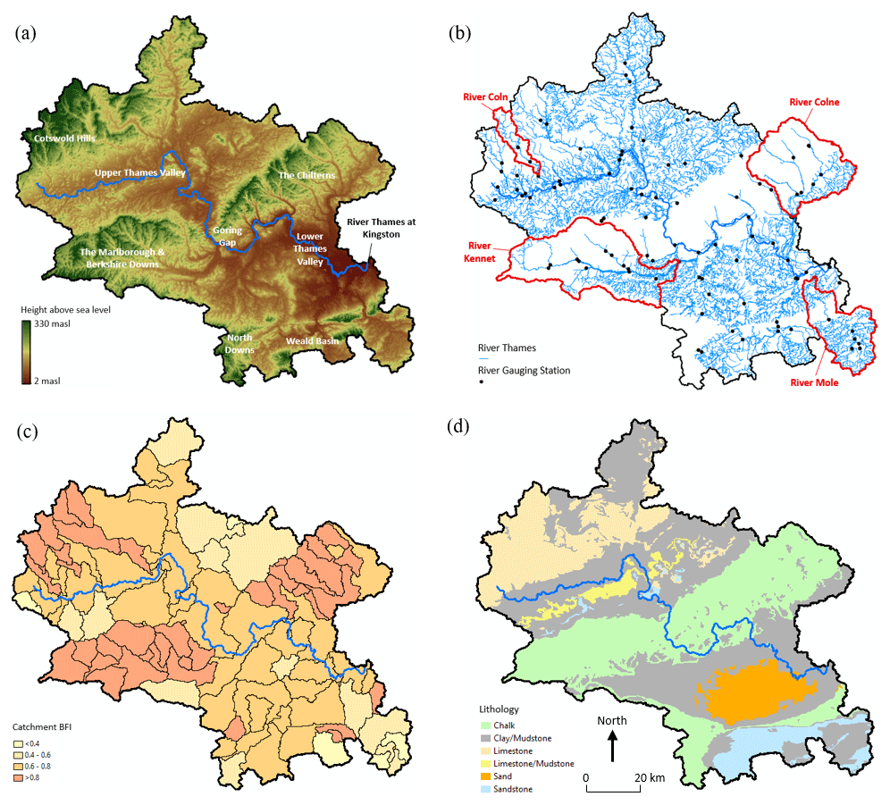
Figure 1Maps of the Thames catchment showing the river Thames at Kingston main river flowing west to east, in relation to (a) the topography and key geographical locations, (b) the river gauging station network and key catchments referred to later in the text, (c) catchment baseflow index (National River Flow Archive (Marsh and Hannaford, 2008)), and (d) main bedrock lithology (after British Geological Survey, 2016). Contains British Geological Survey data © UKRI 2023 and Ordnance Survey data © Crown copyright and database right 2023.
3.1 Data
We use the surface water topographical boundaries delineated by the 102 operational river gauging station networks as our starting point, owing to their use as the delineation basis of surface water catchment models. In this study we refer to a river “reach” as the catchment area between river gauging stations. The analysis undertaken in this study is developed at the river reach scale rather than at the subcatchment scale, as similarly undertaken by Le Mesnil et al. (2020) in their study of the impact of IGF on the water balance of karst catchments in France. This approach has been adopted to avoid increasing averaging or “smoothing” of further downstream metrics, therefore masking small-scale local variation. We collated hydrometeorological, hydrogeological, geological and human influence data in order to undertake the water balance analysis detailed in Sect. 3.2.
3.1.1 Hydrometeorological time series
To characterise the water balance for each reach, daily precipitation, potential evapotranspiration (PET) and discharge for a 21-year period from 1 January 1994 to 31 December 2014 were obtained. Daily rainfall was sourced from the UK Centre for Ecology & Hydrology's (CEH) gridded estimates of areal rainfall (CEH-GEAR) dataset, a 1 km2 gridded product that covers the whole of Great Britain and originates from the Meteorological Office's rain gauge observations (Tanguy et al., 2019). Estimates of daily PET were taken from CEH's climate hydrology and ecology research support system PET dataset (CHESS-PE), which uses the Penman–Monteith equation and is also provided at a 1 km2 gridded scale for Great Britain (Robinson et al., 2016). Reach average rainfall and PET time series were calculated by averaging values of all grid squares that lay within the reach's topographic boundaries described above. Observed daily river flow data were obtained from the National River Flow Archive (NRFA) for all available gauges within the Thames catchment. Additionally, a daily time series of actual evapotranspiration (AET) was calculated by the Thornthwaite (1948) water budget method, based on the reach CHESS-PE potential evapotranspiration series and parameterised with average soil root depths from the work of Lane et al. (2021).
Daily time series of concurrent precipitation, AET and discharge were generated, with a day removed from the analysis if it did not contain all three of these variables of data. When calculating a monthly time series, up to five days of missing discharge data per month were allowed, provided the cumulative rainfall totals on the corresponding days were no greater than 10 % of the total monthly rainfall volume. The missing days were then infilled with the monthly average of that specific month. Average January to December monthly profiles were then calculated, provided there was a minimum of 14 separate months (e.g. Januaries) of data in the time series out of the maximum of 21 in the time period of interest. Unfortunately, this meant that some reaches of key geological interest (e.g. the upper river Lambourn reaches in the river Kennet catchment on the Marlborough & Berkshire Downs Chalk (ref. Fig. 1a and b) were not able to be included in the analysis due to their low data availability; however, a balance had to be made to ensure enough data for robust annual and inter-annual flow calculations. Of the original 102 reaches, 80 remained for use in the following analysis.
3.1.2 Groundwater level time series
Groundwater level data were used to confirm groundwater flow directions (in conjunction with available groundwater level contours) and to investigate the degree of similarity between temporal variations of surface water flows and groundwater levels. Raw data from 1634 boreholes covering the Thames catchment were provided by the Environment Agency, quality assured for units, trends and outliers, and processed into normalised monthly average time series, whereby the minimum groundwater level in an entire time series was subtracted from all the data points in that same time series. Rather than using (often sparse or of variable quality) construction metadata, it has been assumed that a borehole's data reflect the productive aquifer on which it is located. Only boreholes located in reaches with a greater than 70 % coverage of aquifer outcrop were reviewed, as it is on outcrops that groundwater (usually) exerts the most significant influence on surface hydrology. For consistency, the data availability constraints applied during the development of the monthly average groundwater time series were similar to the surface water flow series, ensuring there were a minimum of 14 monthly average data points for each calendar month in the 21-year time series. This left 151 boreholes remaining in the analysis (the locations of which are shown in Fig. 3a). The geographical location of a well within a reach in relation to a river or interfluve etc. was not used as a selection factor, in the interest of keeping as many boreholes as possible in the analysis. It is worth noting that many boreholes have historically only been sampled at a monthly time step; 31 %, 21 % and 48 % of the boreholes had weekly, fortnightly and monthly data respectively. Sensitivity testing was therefore also undertaken on the within-month temporal variability of groundwater levels, and there was minimal effect.
3.1.3 Human influences
Abstractions and discharges can have significant impacts on the evaluation of water balance reach scale calculations. Consequently, such artificial influences should be included in water balance analyses, where possible, to ensure that we do not over or underestimate a reach's water balance characteristics and bias our understanding of IGFs. Surface water abstraction and discharge data were obtained from the CAMELS-GB dataset, which compiled data and information from the Environment Agency (Coxon et al., 2020), and then processed it into reach totals based on the geographic location of the abstraction/discharge. The accumulated abstraction/discharge impacts along a river were calculated and assigned to each reach. There are numerous uncertainties associated with naturalisation methodologies and resulting data, which are discussed in more detail in Sects. 3.2.1 and 6.3. Groundwater abstractions were not included in this analysis, owing to the significant complexities surrounding the associated naturalisation methodologies and the (often sparse) metadata information that would be required. This methodological decision is explained and discussed in detail in Sect. 6.3.2.
3.1.4 Superficial and bedrock geology
The British Geological Survey's 1 : 50 000 superficial and bedrock geology maps (British Geological Survey, 2016) were used to characterise a reach's underlying hydrogeology, by calculating the percentage of aquifer outcrop coverage within each reach. Where the aquifer outcrop coverage in the reach was greater than or equal to 70 % of the total reach area, a hydrogeological classification was assigned. Four hydrogeological typologies were defined: Chalk, Jurassic limestone, Lower Greensand and non-aquifer (i.e. no aquifer outcrop). Dominant lithology has been used previously by Le Moine et al. (2005) in their review of geological variability in relation to the presence of IGF in France.
3.2 Analysis
A perceptual model of IGF across the Thames catchment has been developed using spatial and temporal analysis of water balance metrics and a hydrogeological review of the area. This has allowed us to review the results of the water balance analysis in light of the physical properties of the geology and groundwater systems and thereby identify the location and direction of potential IGF fluxes. We have taken the research decision to qualify, not quantify, IGF. Our overall aim is to identify where water is moving that is not controlled by topography and produce an example high-level perceptual model that could be used by a hydrologist to focus model development flexibly, rather than provide absolute threshold limits for subsurface fluxes. In addition (and as discussed later in the paper), data uncertainties, that are difficult to quantify, reduce the confidence of derived IGF values.
3.2.1 Spatial analysis
Firstly, we reviewed water balance data at a reach scale to quantify the long-term system characteristics of a catchment in relation to its core geological characteristics. The relationship between long-term average precipitation, actual evaporation and river discharge can be used to characterise the water balance of a reach. This long-term water balance (or imbalance) is an important assessment to conduct prior to modelling (Goswami and O'Connor, 2010) and can help to identify catchments with IGF (Genereux et al., 2002; Bouaziz et al., 2018; Le Mesnil et al., 2020) and permanent losses to deep groundwater systems as measurable data on these variables are rarely available.
Following the “watertight catchment” premise which most conceptual rainfall–runoff models follow, assuming a zero-flow condition over the whole boundary, change in storage in the reach over the long term (several years) can be assumed to be negligible (Bouaziz et al., 2018), and the water balance would be presented as
where is the change in reach storage over time, P is the reach areal precipitation, AET is the reach areal actual evapotranspiration, Q is the reach river outflow, Qds is the reach downstream recorded river flow, Qus is the reach upstream recorded river flow (if present) and units are in millimetres per year. The difference between the upstream gauge and the downstream gauge (Q) gives the additional surface water flow contribution from within that reach only. A positive residual of water balance from Eq. (1) can be indicative of a “loss” of water to the reach, where river flow leaving the reach is less than expected from the meteorological data, and conversely a negative residual water balance a “gain” of water to the reach. Aside from uncertainties associated with the input data used in Eqs. (1) and (2) (which are discussed in detail in Sects. 6.3.1 and S2 in the Supplement), the assumption of negligible change in storage at the annual scale can also lead to discrepancies in water balance calculations. Accounting for such discrepancies is outside of the scope of this investigation, in particular as the objective was to identify significant anomalies in water balance outside of disturbance from other terms. To address this, an empirical factor was adopted, whereby only results outside 100 mm yr−1 from a conservative water balance were reviewed (see Sects. 6.3.1 and S3 for further discussion).
Partial naturalisation of river flows was undertaken following the “naturalisation by decomposition” method (Environment Agency, 2001), whereby surface water abstractions and discharges are applied to the recorded river flow record, but groundwater abstractions are excluded from the naturalisation. Whilst this may be an acceptable assumption for many river reaches, even on aquifer outcrops, it certainly will not be true for all (Wendt et al., 2020). It was felt, however, that a more detailed analytical approach involving groundwater abstractions was outside the scope of this study, owing to the complexity of spatially allocating groundwater abstraction impacts to particular river reaches (see Sect. 6.3 for further discussion). Under the assumption that all abstracted water is lost to the system, naturalising the recorded river flow record would result in the water balance equation becoming
where Qnat is partially naturalised reach river outflow, A is reach surface water abstractions, D is reach surface water recorded discharges and units are in millimetres per year.
Whilst the annual average water balance provides a clear losing/gaining assessment of a reach, the non-dimensional representation of reach water balance metrics in relation to the water limit and energy limit considers there to be a wider range of feasible physical characteristics (Le Moine et al., 2007; Andreassian and Perrin, 2012; Bouaziz et al., 2018). The water limit represents the point above which a reach's outflow would be greater than its inflow (i.e. ), a therefore “gaining” reach. The energy limit conversely represents the point below which a reach must be “losing” water as runoff deficits would be exceeding the maximum total PET. This analysis can therefore be used to identify reaches plotting beyond the “natural” range in terms of their water balance.
3.2.2 Temporal analysis
Monthly analysis of the variation in reach responses between the four hydrogeological typologies was undertaken to investigate how seasonal responses vary between different groundwater systems. Reviewing surface water seasonality against local groundwater level seasonality and meteorological variables enables a comparison of the influence of subsurface processes on river flow temporal characteristics. Average October to March monthly profiles were developed for each reach in each geology, covering effective rainfall (precipitation minus actual evapotranspiration), groundwater level and river discharge. A comparison between the seasonal highs and lows of the different variables was undertaken. Whilst this is not an intra-annual analysis of IGF (owing to difficulties surrounding the influence of storage), this information supports hydrological modellers in developing their understanding of reach characteristics and offers useful information as to the variation between reaches on different hydrogeological typologies.
3.2.3 Hydrogeological analysis
Local scale analysis and interpretation of meteorological, hydrological and hydrogeological data allow the hydrologist to refine a reach-focussed perceptual understanding. The literature states that a reach's water balance (Bouaziz et al., 2018), its location upstream (Fan, 2019) and the presence of permeable substratum (Le Moine et al., 2005) can all assist in the identification of reaches with IGF. These IGF “indicators” can be used as a perceptual “roadmap” (such as per Fig. 2), whereby the hydrologist can query a reach's water balance result in terms of its likelihood to be due to IGF processes. Figure 2 can therefore assist with the high-level identification and explanation of both expected and unusual water balance reach characteristics. We propose using these IGF indicators from the literature as an initial starting point for the identification of IGF, but developing this further via a more detailed hydrogeological analysis, whereby we then look at the supposed physical feasibility of IGF in identified non-conservative reaches in comparison to aquifer outcrop boundaries (Pellicer-Martinez and Martinez-Paz, 2014), aquifer properties, the local groundwater flow direction (Toth, 1963) and the presence of springlines (Frisbee et al., 2016), in areas where we see losing and gaining reaches. This would develop a more detailed reach-specific understanding of the groundwater environment and provide additional evidence of IGF. A final perceptual model of the Thames catchment is then presented in Sect. 6.1, drawing on the water balance results in conjunction with the hydrogeological evidence analysed.
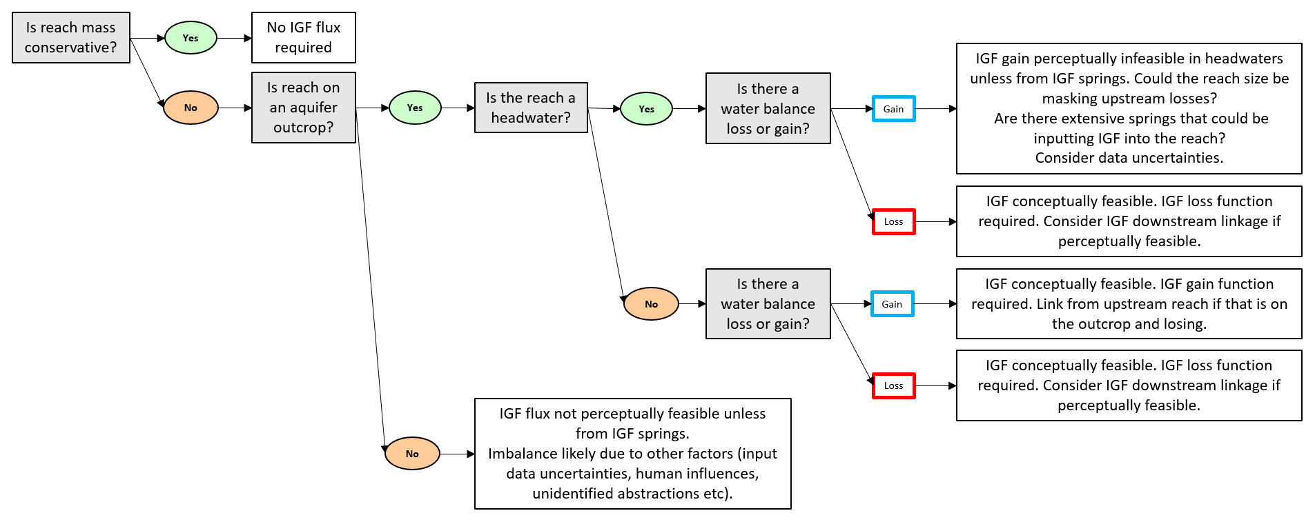
Figure 2Perceptual roadmap for high-level initial identification of river reaches with possible intercatchment groundwater flow, from a physical process-based assessment. Note that more than one process may be at work in a single reach, e.g. both incoming IGF from upstream river reaches and outgoing IGF to downstream river reaches.
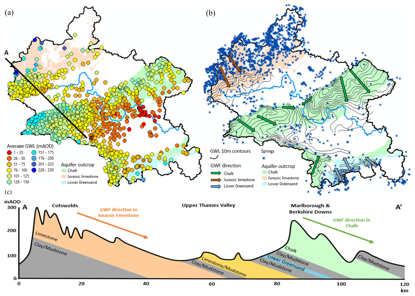
Figure 3Hydrogeological features and characteristics of the Thames catchment showing (a) average groundwater levels and the location of the geological cross section in (c); (b) the location of springs (digitised from Ordnance Survey mapping), general “median” aquifer groundwater level contours (after Atkins, 2003, 2007; Entec UK Ltd., 2008; Environment Agency, 2010 and ESI Ltd., 2013), and flow direction arrows in relation to aquifer outcrop areas; and (c) a geological cross section showing the three main aquifers, simplified lithology, and general groundwater flow direction. Contains British Geological Survey data © UKRI 2022 and Ordnance Survey data © Crown copyright and database right 2023.
To fully understand IGF across the river Thames Basin we need to first undertake a local analysis of the geology and hydrogeology. This information is imperative in supporting any conclusions as to the presence of IGF in a study area.
The geology of the Thames is highly heterogenous. The geological strata at the surface become progressively younger from north-west to south-east across the catchment (Fig. 3c) and give rise to “scarp and vale” topography (Lane et al., 2008). Superficial deposits are not continuous (although they may be hydrogeologically significant at the river reach scale; Bloomfield et al., 2011; Bricker and Bloomfield, 2014). There are three principal aquifers within the Thames Basin: the Chalk, the Jurassic oolitic limestones and the Lower Greensand (Fig. 3). The groundwater in these aquifers is separated by lower permeability geological strata (Fig. 3c) and so, for the purposes of perceptual modelling, can be considered to be disconnected, complicating the regional groundwater flow framework of Toth (1963), as there will not be a Thames catchment-wide groundwater flow system. There will, however, be aquifer-wide groundwater flow systems which may link surface water catchments that are situated on the same aquifer outcrop via IGF pathways. The groundwater level data in Fig. 3a and contours in Fig. 3b show groundwater flow at the aquifer scale is generally towards the south-east, with the exception of the Lower Greensand, in which flow is towards the north-west (Fig. 3b). The aquifer properties of the three aquifer units are summarised in Table 1.
Table 1Range of hydraulic aquifer properties (where available) of the main aquifers in the Thames catchment after Allen et al. (1997) and Bloomfield et al. (2011). It should be acknowledged that the storage values reported below may relate to both confined (elastic) storage coefficients and specific yield values, depending on the approach taken to analyse the pumping tests on which they are derived. This may be particularly likely in the Chalk.

4.1 Jurassic limestone
Groundwater is present in both the lower Inferior Oolite and upper Great Oolite Jurassic limestones of the Cotswold Hills, which are in direct hydraulic contact in some areas and separated by the 20–30 m thick mudstone aquiclude of the Fuller's Earth Formation in others (Bricker et al., 2014). The Jurassic limestones have low matrix porosities, are well cemented and have low intergranular permeability but are highly fractured, faulted and fissured (Allen et al., 1997). Consequently, the aquifer has a high transmissivity and a median storage coefficient similar to that of the Lower Greensand but is 2 orders of magnitude lower than the equivalent for the Chalk (Table 1). Groundwater flow is predominantly along preferential flow paths, and groundwater levels respond rapidly to rainfall (Newmann et al., 2003). The aquifer extends across a number of river subcatchments (see Fig. 1c for distribution of subcatchments). Given the high transmissivity and presence of numerous springs across the outcrop, in particular in the upper reaches (Fig. 3b), perceptually there is the potential for IGF from one subcatchment to another. The location of many springs just outside of the study area, to the north-west of the topographical surface water watershed boundary, could be suggestive of IGF out of the Kingston catchment.
4.2 The Chalk
The Chalk outcrop covers 29 % of the study area and contains over 20 river subcatchments (see Fig. 1c). The Chalk aquifer is the most important groundwater resource in Great Britain (Allen et al., 2010) and makes up over 50 % of total groundwater abstraction (Shand et al., 2003b). It is a fine-grained, microporous limestone, which has a high matrix porosity, but low matrix conductivity because of the small pore sizes (Butler et al., 2012). It is the Chalk's extensive fracturing that gives it its high transmissivity (Table 1) and through which saturated flow occurs. The fracture network also provides its drainable porosity; typically specific yield is in the range of 0.5 %–2 %. Dissolution of the Chalk within the zone of water table fluctuation, and periglacial weathering, which has preferentially occurred in valleys, have enhanced the fracture network and given rise to significant vertical and horizontal heterogeneity. The extent of groundwater–surface water interaction across this geological unit will therefore be highly variable, dependent on very localised physical conditions of the Chalk. Bulk hydraulic conductivity generally decreases with depth, and transmissivity reduces away from river valleys (Allen et al., 1997). There is a clear sparsity of perennial rivers on the Chalk outcrop (Fig. 1b), indicating a predominance of groundwater flow mechanisms (Adams, 2008). Given these physical attributes, the groundwater flow network across the aquifer will be having a significant impact on the surface water hydrology. Springlines are evident along the outcrop boundaries, particularly along the north-western escarpment of the Chalk (Fig. 3b), where the groundwater contours in Fig. 3b show localised northerly groundwater flow off the Chalk outcrop. This is likely causing IGF into the upper Thames Valley.
4.3 Lower Greensand
The Lower Greensand Group comprises two main hydrogeological units – the Hythe Formation and the uppermost Folkestone Formation, which, being separated by an aquitard layer, can be considered two separate aquifers (Allen et al., 1997). Intergranular flow is the primary flow mechanism, along with fracture flow (Shand et al., 2003a). Bloomfield et al. (2011) noted that limited seasonal variation in groundwater heads in the Lower Greensand is associated with relatively high storage compared with the stratigraphically adjacent Gault and upper Jurassic clay formations. There is a greater density of drainage channels on the Lower Greensand than the Chalk or Jurassic limestone outcrops (Table 1 and Fig. 1b) and a concentration of springs in the upper reaches (Fig. 3b). Owing to the lower river incision and transmissivity (Table 1), the impact of groundwater–surface water interaction on the river flows in subcatchments located on this outcrop may be less than on the Jurassic limestone and Chalk aquifer outcrops.
5.1 The spatial variation of annual water balance metrics
Figures 4, 5 and 6 present the spatial variation in average annual water balance metrics (1994–2014) across the Thames catchment. The results are discussed with reference to the hydrogeological review undertaken in the previous section. Whilst catchment (rather than reach) metrics have not been presented as a part of this analysis, it is of note that the average annual naturalised water balance of the whole Thames catchment is near to conservative, at only 5 % of the average annual precipitation.
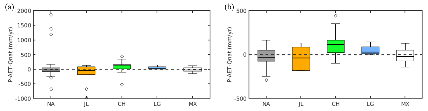
Figure 4Distribution of annual average reach water balance metrics for each lithology for the Thames at Kingston reaches from 1994–2014 inclusive, showing unaccounted for annual water volume from precipitation after subtraction of actual evapotranspiration and naturalised river flow (in millimetres per year). A positive water balance residual indicates a losing reach and a negative water balance residual a gaining reach at the annual time scale. The boxes show the interquartile interval, within which 50 % of the data lies, and the horizontal line the median value. The whiskers show the minimum and maximum values, excluding outliers. The plot in (a) shows all data and the plot in (b) is focussed in to ±500 mm yr−1, thereby excluding some wider outliers. Reaches have been categorised based on > 70 % catchment geological coverage. CH: Chalk (n=23), JL: Jurassic limestone (n=11), LG: Lower Greensand (n=4), NA: non-aquifer (n=28) and MX: mixed (n=14).

Figure 5Annual average reach water balance metrics for the Thames at Kingston from 1994–2014 inclusive, showing unaccounted for annual water volume from precipitation after subtraction of actual evaporation and naturalised river flow (in millimetres per year), in relation to aquifer outcrop areas and median groundwater level contours for the same time period. A reach where the water balance residual is within 100 mm of balanced is considered to be conservative, to nominally account for data uncertainties (see Sect. 6.3.1). Catchments referred to in the text are outlined in red.
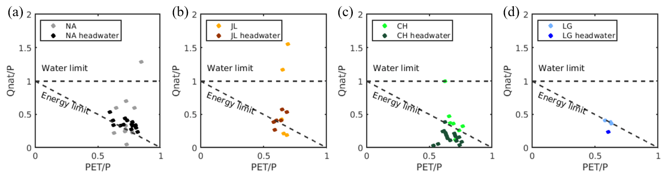
Figure 6Annual average reach water balance metrics for the Thames at Kingston reaches from 1994–2014 inclusive, showing dimensionless reach runoff coefficient (river flow/precipitation) and dryness index (potential evapotranspiration/precipitation) in relation to the water limit, the energy limit and their headwater (i.e. no upstream gauge) or “non-headwater” location along the river, under naturalised conditions. Reach categorisations are based on > 70 % catchment geological coverage of NA: non-aquifer (n=28), JL: Jurassic limestone (n=11), CH: Chalk (n=23) and LG: Lower Greensand (n=4). The results from the three Lower Thames reaches are not shown on panel (a) as they have negative reach runoff coefficient results.
There is minimal difference between the non-naturalised and the naturalised reach results (Figs. S4, S5 and S6), with a non-conservative water balance of > 100 mm yr−1 being “corrected” by naturalising the discharge series in only 3 of the 80 reaches. For the purposes of the current analysis, focus is given to the naturalised results only, owing to their similarity to the non-naturalised results. The non-naturalised results are shown for information in the Supplement. The three lowest main river reaches show particularly large naturalised water balance losses (> 1000 mm yr−1) (Fig. 5). In a catchment as heavily artificially influenced by abstractions and discharges as the Thames at Kingston (Environment Agency, 2018b), this raises questions as to the completeness of the naturalisation data or the effectiveness of the employed naturalisation methodology. This is discussed further in Sect. 6.3.
The naturalised results show variability in annual water balance between the main hydrogeologies – non-aquifer areas, Jurassic limestone outcrop, Chalk outcrop and Lower Greensand outcrop (Fig. 4). With the exception of the three lowest main river Thames reaches near Kingston, annual reach losses are only observed on aquifer outcrop areas (Fig. 5), where the recorded river flow is less than expected given the meteorological variables. Sixty percent of the greatest water balance losses (> 100 mm yr−1) observed in the Thames catchment are on the Chalk outcrop, where there is an average reach loss of 187 mm yr−1. The Lower Greensand reaches show smaller water balance losses on average (51 mm yr−1) (Fig. 4), with only one of the four reaches exhibiting a loss of more than 100 mm yr−1 (Fig. 5). The Jurassic limestone reaches gain water on average (average water balance of −156 mm yr−1) although there are some reaches with large losses (Fig. 4). Again with the exception of the three lowest main river Thames reaches, non-aquifer reaches are gaining water at the annual scale on average (−60 mm yr−1) (Fig. 4). The results highlight significant variability within, not just between, the aquifer outcrop geologies. Recognising the small sample sizes and associated uncertainty, the Jurassic limestone reaches show the greatest range of naturalised annual average water balances (interquartile range of 228 mm yr−1 (n=11) compared to a range of 150 mm yr−1 on the Chalk (n=23) and 112 mm yr−1 on the Lower Greensand reaches (n=4)).
Reaches with negative annual water balances (gains) tend to be seen downstream of reaches with positive water balances (losses) (Fig. 5). The Chalk reaches show a pattern of headwater catchments consistently losing (plotting below the energy limit) and non-headwater catchments gaining water at the annual average scale (Figs. 5 and 6c). For example, the rivers Kennet and Colne on the Chalk (ref. Fig. 1b) have annual average water balance losses in their headwater reaches and gains further downstream. There is a 125 mm yr−1 average annual loss in the Kennet Chalk headwater reaches (equivalent to 15 % of average annual rainfall in these reaches) and gains along the Kennet main river reaches (equivalent to 38 % of the average reach rainfall) (Fig. 5). This is at the southerly limit of the Chalk aquifer outcrop, where it becomes overlain by the less permeable clay material of the upper/lower Thames valleys (illustrated in Figs. 1c and 3). This pattern of losing headwater reaches to gaining downstream reaches can also be seen in the river Coln on the Jurassic limestone and river Colne on the Chalk (ref. Figs. 1b and 5).
5.2 The temporal variation of annual water balance metrics
There is little difference in the seasonality of effective rainfall between the different geologies (Fig. 7a–d) across the Thames Basin, but the intra-annual temporal variability of reach average discharge and groundwater levels (Fig. 7e–k) does vary, illustrating the differences in the physical aquifer properties of the three hydrogeological units.
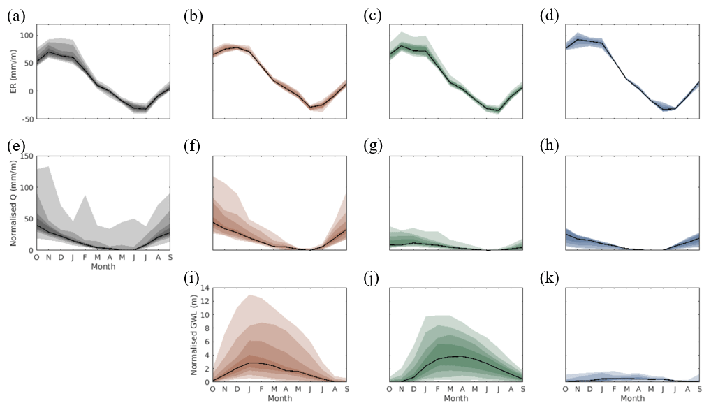
Figure 7Seasonal patterns of (a–d) effective rainfall (P−AET), (e–h) normalised naturalised discharge and (i–k) normalised groundwater levels for non-aquifer, Jurassic limestone, Chalk and Lower Greensand reaches (in shades of grey, orange, green and blue respectively). Reaches have been categorised based on a minimum of 70 % geological aquifer outcrop coverage at the surface. The dark black lines show the mean of the data and the shaded bands represent the 95th, 85th, 75th and 65th percentiles of the data.
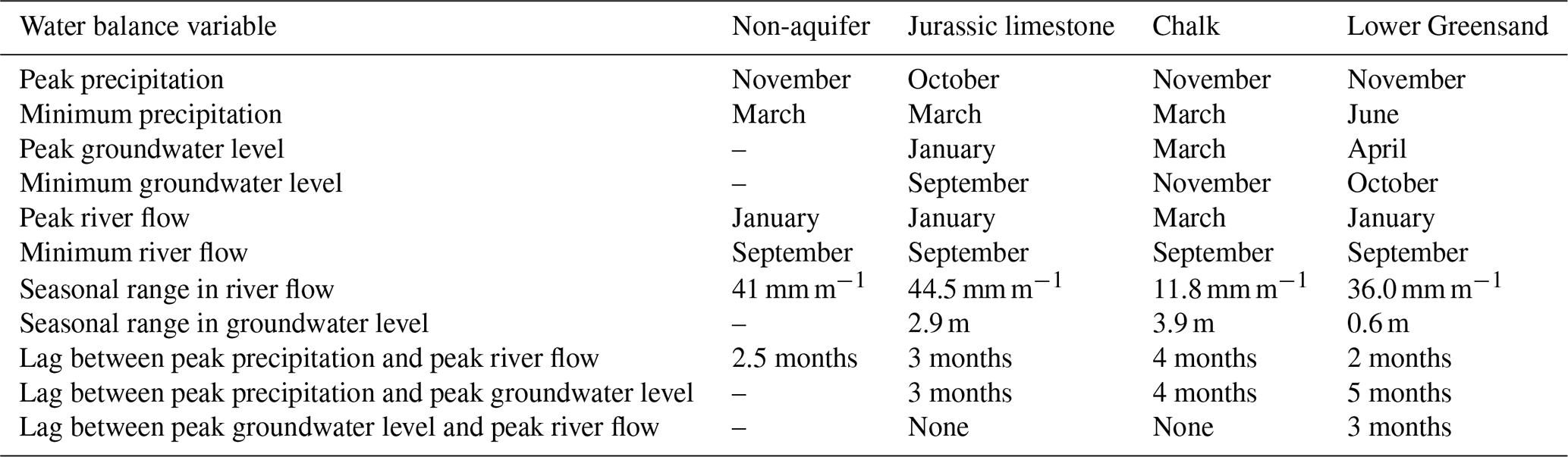
The Lower Greensand annual average groundwater hydrographs are particularly muted (Fig. 7k), with minimal monthly variation in groundwater level (only a 0.6 m seasonal average range, in comparison to the 2.9 and 3.9 m range in the Jurassic limestone and Chalk respectively – Table 2) and a particularly flat seasonal river flow profile (Fig. 7h) (Shand et al., 2003a).
The Chalk reaches also show flat seasonal discharge profiles (Fig. 7g and Table 2), with the exception of one reach – the mid-reach on the river Kennet, which gains significant flow (see Fig. 5). The Chalk reaches show a delayed onset of winter higher groundwater levels (March) in comparison to reaches on the Jurassic limestone (January), which is reflected in a delayed winter river flow peak (Fig. 7g, black line). The lag between rainfall and river flow is the longest of the geologies (Table 2). The signal of precipitation in the river flow record on the Chalk is, on average, a 4 month lag between average annual peak precipitation and average annual peak discharge (Table 2).
Rivers on the Jurassic limestone exhibit the greatest monthly variability of the three hydrogeological units (Fig. 7f and Table 2), reflecting the groundwater trends within that geological unit (Fig. 7i). River flow seasonality on the Jurassic limestone mirrors the highly responsive groundwater levels.
Table 2Seasonality and lags of the 50th percentiles of precipitation, groundwater level and river flow. Reaches categorised based on a minimum of 70 % geological aquifer outcrop coverage at the surface.
6.1 The Thames perceptual model
The perceptualisation process (illustrated in Fig. 2) enables us to recognise where IGF processes may be occurring. This highlights the need for a degree of local investigation and hydrogeological perceptualisation (Le Moine et al., 2005) within the regional analysis. Drawing on the findings from the analysis in the previous section, coupled with the hydrogeological review in Sect. 4, a groundwater–surface water regional perceptual model of the Thames catchment (from the perspective of a surface water modeller) is provided below, and summarised in Fig. 8.
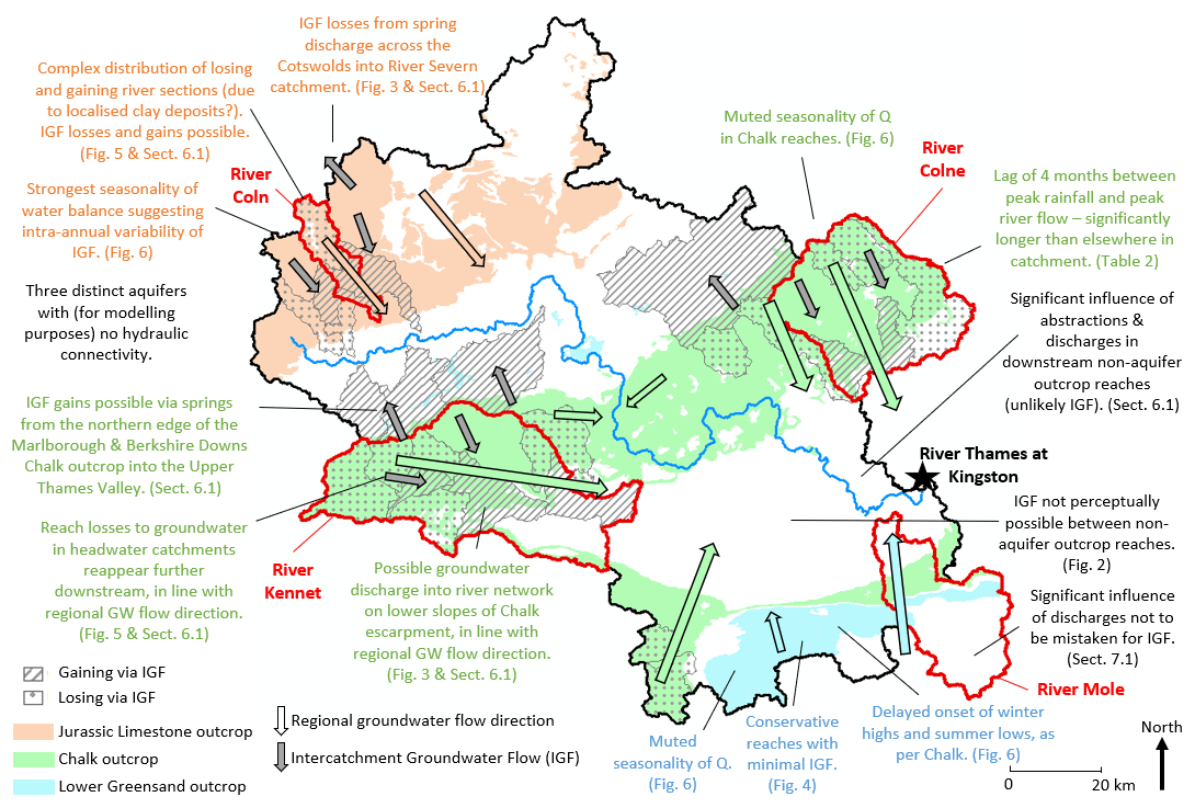
Figure 8Perceptual model of the Thames catchment, including key modelling-related groundwater–surface water interaction features and characteristics. The Jurassic limestone, Chalk and Lower Greensand aquifers are (for modelling purposes) hydraulically disconnected. Contains British Geological Survey data © UKRI 2023.
Through analysis of recorded hydrometeorological water balance data we have shown the prevalence of non-conservative reaches across the Thames catchment, both gaining and losing. This has also been found by numerous authors in their analyses of annual water balance metrics, for example in France (e.g. Le Moine et al., 2007; Andreassian and Perrin, 2012; Bouaziz et al., 2018; Le Mesnil et al., 2020) and the USA (e.g. Schaller and Fan, 2009).
The spatial variability of non-conservative reaches has shown heterogeneity both between, and within, geological units. The significant heterogeneity of the Chalk (Bloomfield, 1996; Upton and Jackson, 2011) gives rise to both recharge and discharge points along river courses and, potentially, within river reaches (Butler et al., 2012). In the Jurassic limestone, faulting and spatial variability in the thickness of the Fuller's Earth Formation (Sect. 4.1) between the Inferior and Great Oolites, and the large number of consequential springs (Fig. 3b), are leading to a complex distribution of discharge points across the outcrop (Newmann et al., 2003). Although the sample size of the Lower Greensand reaches is small (n=4), we found limited variability in water balance results between the Lower Greensand reaches which is in line with the recorded transmissivities for that unit being both smaller and of less variability than those found in the other geologies (Allen et al., 1997).
Fan (2019) recommends using the “hydrologic signals” of adjacent losing to gaining reaches and the presence of spring clusters to help identify IGF. Given the high porosity and extensive fracturing of Chalk (Sect. 4.2) (Bloomfield, 1996) and the observed loss-to-gains in flow (Fig. 5b), which coincide with the regional groundwater flow directions depicted from average groundwater level data and contours in Fig. 3, it can be inferred that the “lost” water in the upper Chalk reaches is flowing into adjacent downstream reaches via the groundwater flow system. This is supported by the literature (Allen et al., 1997; Shand et al., 2003b). Examples can be seen in the rivers Kennet and Misbourne (Fig. 5b) where water balance gains are observed as a result of local connectivity of geological units and the presence of springs along the contact of the Chalk and the overlying clay/mudstone (Fig. 3b) (Upton and Jackson, 2011).
In the literature, much research has looked at IGF in karstic environments (e.g. the work in France by, amongst others, Bouaziz et al., 2018; Le Mesnil et al., 2020, 2021). The Chalk of the Thames catchment can be locally sub-karstic (Maurice et al., 2006; Bloomfield et al., 2009), but because the rock mass exhibits a pervasive and dense fracture network (Mortimore, 2012) flow through these is the primary groundwater flow process (Allen et al., 1997). Whilst the regional groundwater flow direction in the Chalk is to the south-east, localised northerly groundwater flow will be discharging Chalk groundwater from headwater reaches of the river Kennet into the “non-aquifer” reaches of the upper Thames Valley (Upton and Jackson, 2011) (see Fig. 3b groundwater contours and Fig. 1a). Whilst not impacting the water balance beyond 100 mm yr−1 (and so not showing in Fig. 5b), the reaches just to the north of the Marlborough & Berkshire Downs Chalk do exhibit water balance gains of 70–80 mm yr−1, which are likely attributable to northwards IGF (ref. the perceptualisation roadmap in Fig. 2).
Karstic flow has also been reported in the Jurassic limestone (Allen et al., 1997). IGF will likely be occurring in this unit via fracture pathways (Bricker et al., 2014) and from the springs to the north-west (into the adjacent river catchment to the Thames, the river Severn (ref. spring locations in Fig. 3b); see Fig. 8). This is supported by the literature (e.g. Newmann et al., 2003). The relationship between the Inferior and Great Oolite units is complex, and cross-catchment flow has been confirmed (Bricker et al., 2014). Our results mirror this, particularly in light of the spatially variable nature of the losses and gains observed at the annual water balance (Fig. 5b).
From the above, we can attribute “large-scale” non-conservatism of reaches on the Chalk and Jurassic limestone to IGF, but this is not evident on the Lower Greensand reaches, which are largely conservative. Additionally, and crucially, water balance imbalances on non-aquifer outcrop reaches should not be attributed to IGF (unless located adjacent to an aquifer reach and down gradient of local groundwater flow, e.g. the spring flow into the upper Thames Valley discussed above) (as we have assumed in the perceptualisation roadmap in Fig. 2).
In addition to the IGF identification above, our results also provide information on the monthly profile variations of water balance metrics (effective rainfall and river discharge) and groundwater levels between the different geologies in our study area. Geology influences lag timescales (Marchant and Bloomfield, 2018; Fowler et al., 2020), with river flow seasonality showing a high level of influence of catchment storage. Our water balance metric temporal results demonstrate lag times of 4 months between peak rainfall and river flows for Chalk reaches, in line with other studies (Weedon et al., 2015). The longer seasonal lags observed on the Chalk in comparison to the Jurassic limestone (Table 2) will be due to the lower transmissivity coupled with high storage of that unit (Table 1). Whilst rapid flow through fractures can occur (Upton and Jackson, 2011), unsaturated flow through the Chalk is predominantly via the matrix, resulting in recharge of the water table via the displacement mechanism (Ireson et al., 2006). It is this process that is being principally observed in the relatively muted and delayed seasonal groundwater level hydrographs and, consequently, the surface water hydrographs in Fig. 7g and j.
The Jurassic limestone groundwater levels exhibit the greatest seasonal variation of the geologies, owing to the low storage of the aquifer but high transmissivity (Bricker et al., 2014) (Table 1), as higher groundwater levels in the winter months give rise to the highest transmissivities and greater groundwater flow, but under drier conditions the opposite would occur. The presence of rapid flow pathways to the heavily incised (Table 1) rivers on that outcrop, via fractures and faults, results in a strong seasonal control on the river flow annual profile (Fig. 7f) (Newmann et al., 2003; Bricker et al., 2014) that is not observed on the Chalk or Lower Greensand.
In our example study, the high specific yield of the Lower Greensand aquifer gives rise to observed steady groundwater heads (Shand et al., 2003a; Bloomfield et al., 2011) (Fig. 7k) and, combined with the high connectivity to the river drainage network via diffuse groundwater flow (Bloomfield et al., 2011), this is replicated in the muted seasonality of the Lower Greensand reaches' river flow profiles (Fig. 7h).
This perceptual model is the key output of the perceptualisation approach advocated by this paper, incorporating both surface water and groundwater processes via an evidence-based objective analysis at the local reach scale. It is this output that we advocate being used by surface water modellers to aid with hydro(geo)logically appropriate model set-up, development and calibration.
6.2 Are current modelling approaches fit for purpose and how might we change them?
Not including IGF as a model flux will result in many models overestimating river flows or actual evapotranspiration (Bouaziz et al., 2018; Fan, 2019) in an effort to “close” the water balance in groundwater-dominated catchments. It is well known that the “watertight substratum” assumption on which so many of our conceptual catchment rainfall–runoff models are built is frequently unrealistic in terms of the actual physical processes occurring (Le Moine et al., 2005; Wanders et al., 2011; Bouaziz et al., 2018; Fan, 2019), as many of the key assumptions used to simplify a complex catchment (i.e. that of a clear boundary condition at the watershed and a lower no-flow boundary condition at bedrock) do not hold for permeable, groundwater-dominated catchments. We have the opportunity to develop the physical realism of these models and improve their simulation but, crucially, in line with available evidence. We need to advocate different modelling approaches, with flexibility being a key principle. Allowing high-resolution compartmentalisation (e.g. hydrological response units) of different process representations would enable the modeller to address the heterogeneity between different geologies and, even, within geologies at the sub-reach scale.
The extent of non-conservative reaches across our study area supports the application of external subcatchment flux(es) (loss functions) to represent IGF, as previously advocated by Le Moine et al. (2007), Pellicer-Martinez and Martinez-Paz (2014), and Yang et al. (2017). We have, however, shown IGF to vary in time and space as a function of hydrogeological control. IGF may not be perceptually justified in all subcatchments and should therefore be supported by prior perceptualisation investigations to inform decisions on flux flow direction, connectivity, variability and spatial location. As such, we would not advocate the use of uniformly parameterised loss functions, where they are applied across all catchments in the same way. Parameterisation of IGF fluxes could be based on lithology, as suggested by Le Moine et al. (2005), or groundwater data (depending on data availability).
Loss functions should be linked between catchments where possible and hydrogeologically feasible (as highlighted by Pellicer-Martinez and Martinez-Paz, 2014). Groundwater flow is a process that occurs between surface water catchments and should be represented as such to reduce the risk of a model using such a flux as a simple “fudge factor” to improve calibration (as warned by Le Moine et al., 2005, and Goswami and O'Connor, 2010). Flow accretion can show a longitudinal train of gaining and losing reaches, as shown by our reach-based analysis (Fig. 5). Considering such reaches as separate, independent entities with independent IGF fluxes would misrepresent the hydrological processes occurring and could give rise to unfeasible parameterisation during model calibration.
The intra-annual variability of groundwater processes can be significant, based on natural cycles of meteorological and surface water variables. In addition, groundwater levels may be seasonally affected by abstractions (e.g. for agriculture). Whilst not explicitly investigated in this paper, it is likely that this temporal complexity will mean that water balance losses/gains via IFG are unlikely to be temporally continuous and so should not be represented as a constant loss with no seasonal variation. Whilst it is acknowledged that temporal variation is not always seen within IGF (both Yang et al. (2017) and Zanon et al. (2014) found a temporally steady groundwater model flux to be successful for model calibration (although this was not linked back to the hydrogeological processes controlling the flux)), a constant value of flux should only be applied when the evidence and perceptualisation support this.
6.3 What are the challenges and limitations in perceptualising?
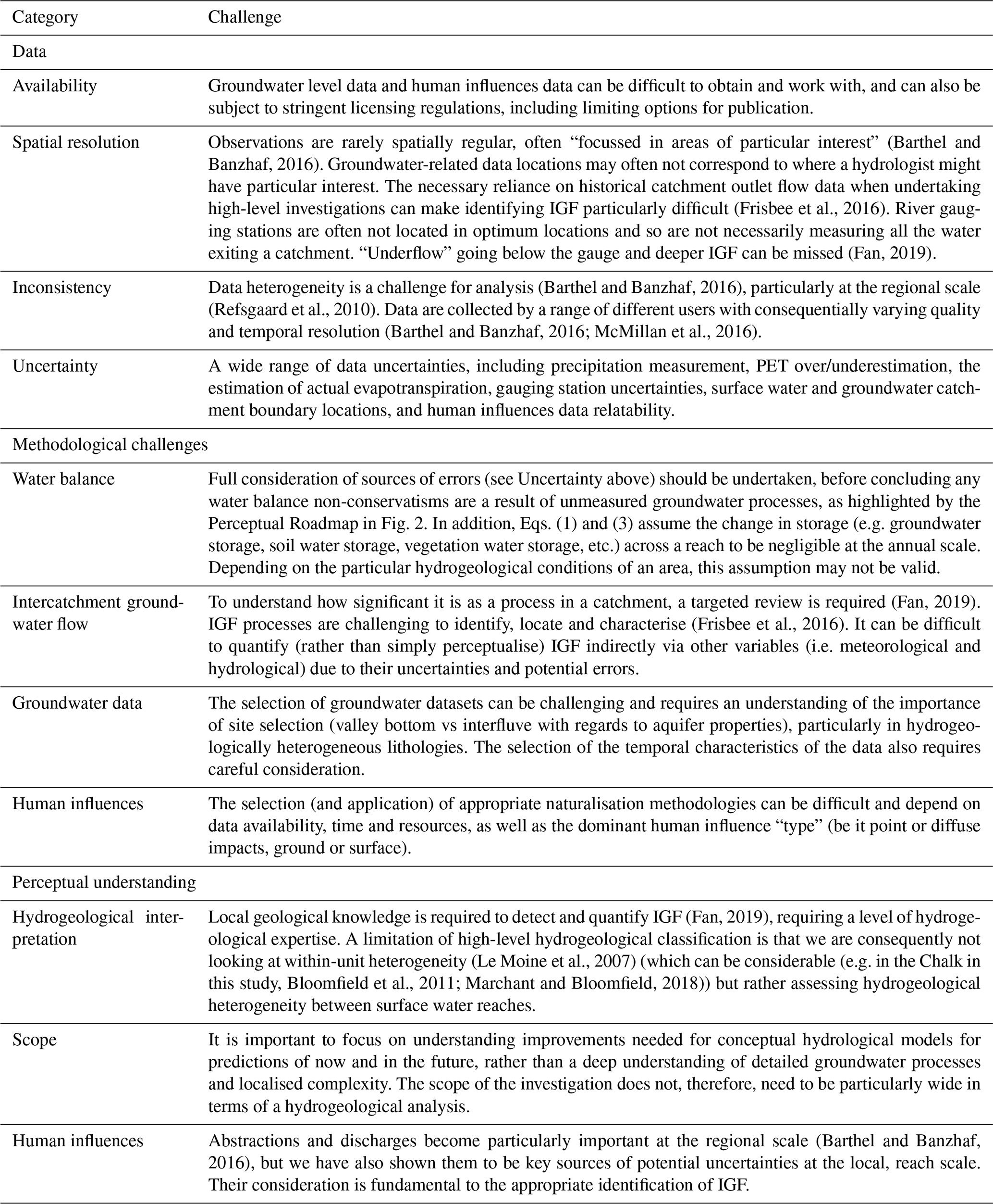
The measurement of IGF fluxes is rarely feasible (Le Moine et al., 2007; Frisbee et al., 2016), although there are examples of field studies attempting this e.g. Käser and Hunkeler (2016) and Genereux et al. (2005). Table 3 summarises the challenges faced when trying to perceptualise IGF, linking hydrological and hydrogeological data and varying spatial scales, categorised into data challenges, methodological challenges and perceptual understanding challenges. Two key challenges (those of uncertainties and naturalisation) are discussed in more detail in the following sections.
Table 3Matrix of challenges when developing a perceptual model of the intercatchment groundwater flow environment for the purposes of improved hydrological modelling, split by challenge category.
6.3.1 Input data uncertainties
As detailed in Table 3, the perceptualisation of IGF introduces a wide range of data uncertainties, and care needs to be taken to ensure that data anomalies are not mistakenly attributed to IGF (as Bouaziz et al., 2018, and Zanon et al., 2014, warn in the case of input data uncertainties). Whilst a full quantification of uncertainties may be beyond the scope of an IGF perceptualisation when for the purposes of informing model editing, it is important to reflect on the uncertainties being introduced. We have summarised some of the available literature on input data uncertainties relevant to this paper below.
In the case of catchment areal precipitation and PET estimation, the error source is two-fold: sample measurement errors and spot-data interpolation method errors (McMillan et al., 2012). When using a gridded rainfall data product such as CEH-GEAR (which has undergone extensive raw data and interpolation quality control procedures, Tanguy et al., 2019), the largest errors associated with the data originate from the raw rain gauge measurements, in particular relating to wind loss, resulting in under-catch (5 %–16 %, McMillan et al., 2012; Keller et al., 2015). However, the magnitude of these errors is reduced when there is a high rain gauge network density (Keller et al., 2015), such as in the data-rich Thames catchment.
The uncertainties surrounding potential evaporation are complex due to its basis on underlying empirical equations involving a number of separately recorded (or estimated) variables. The potential errors associated with the FAO Penman–Monteith method (on which the CHESS-PE dataset is based, Tanguy et al., 2019) have been reviewed by a number of authors and shown to vary through the calendar year due to its sensitivity to potential errors in the temperature variable (Talebmorad et al., 2020). Estimates of average potential evaporation error using the FAO Penman–Monteith method have been recorded as 10 % (Talebmorad et al., 2020), 5 %–10 % (Hua et al., 2020) and 10 %–40 % (Westerhoff, 2015). The conversion of PET to AET introduces further uncertainties owing to its greater complexity (Westerhoff, 2015). The Thornthwaite (1948) method adopted in this study incorporates the precipitation and PET data (and their associated errors), as well as estimation of soil water stock (Sect. 3.1.1). Estimates of actual evaporation uncertainties have been calculated to be between 10 % and 11 % (Price et al., 2007; Jakimavičius et al., 2013).
Discharge uncertainties from river gauging stations vary depending on measurement method (McMillan et al., 2012) and can vary over time (Coxon et al., 2015). Assessment of their errors is complicated by often lacking metadata on the structure and stage to discharge calculation methods (Coxon et al., 2015). In the Thames, weir calculations are most prevalent (Coxon et al., 2015). Errors in mean time-averaged daily flow measurements can range from 10 % to 20 % (McMillan et al., 2012). Assessing discharge over a long time period and incorporating periods of varying climatic conditions can help increase confidence.
As part of our analysis methodology, we have assumed that average non-conservative reach water balance discrepancies greater than 100 mm yr−1 (from Eq. 3) (equivalent to 14 % of the annual average rainfall in the Thames catchment, Marsh and Hannaford, 2008) can be assumed to be attributable to factors other than input data uncertainties. It must be clearly acknowledged that the setting of this threshold is arbitrary, however we believe its selection to be robust. To support this methodological decision, we firstly undertook a high-level quantification of potential water balance uncertainty based on precipitation, actual evapotranspiration and river discharge errors; and we secondly undertook sensitivity testing of the selection of the threshold value (see Sects. S2 and S3). As reported in Sect. S2, our estimates of maximal water balance uncertainties attributable to input data were in the order of ±30 mm yr−1, and thus considerably below our 100 mm yr−1 threshold. We adopted such a conservative threshold to reflect our acknowledgement of our calculated error distributions being based on limited papers and a given error model, selecting only the clear cases of high water balance errors for further investigation. Future work could focus on investigating and quantifying other potential sources of water balance errors, as per those detailed in Table 3, to further improve upon water balance estimations.
6.3.2 Naturalisation
A notable challenge that we have found in this study is that of the influence of human abstractions and discharges. The process of river flow naturalisation is itself one of great uncertainty (Terrier et al., 2020). In Fig. 5b, both > 100 mm yr−1 water balance losses and gains have been calculated in non-aquifer reaches, most notably the three lower Thames reaches and along the river Mole (ref. Fig. 1b). Following the perceptualisation roadmap in Fig. 2 regarding the absence of aquifer outcrop coverage and springlines, we can deduce that these “non-conservatisms” are not due to IGF processes and investigate alternative causes. It is known that major public water supply abstractions (lower Thames) and discharges (river Mole) are located in these reaches. The relative scale of these artificial influences in relation to the increase/decrease in river flow between gauging stations is leading to anomalous water balance results. This highlights a disadvantage and challenge of using reach-based analysis when applying naturalisation.
In addition, our naturalisation method explicitly discounts groundwater abstractions. In a study area with known abstractions from nationally important aquifers (Butler et al., 2012), this assumption is obviously flawed. However, it must be acknowledged that a full naturalisation incorporating both surface and groundwater abstractions and discharges would be a significantly time-consuming and data intensive. Quantifying the impacts of groundwater abstractions on river flows is challenging (Ivkovic et al., 2014) and more complex than that of surface water influences when, in particular, identifying the location of any consequential reduction/modification of flow (Coxon et al., 2020). Much groundwater abstraction is for irrigation use and the return of such abstracted water to the river from runoff or shallow surface flow would also need to be considered. Equating groundwater abstraction to an actual loss in river flow (e.g. rather than for the purposes of stream support) adds further complexity and detailed knowledge of (often confidential) abstraction licence conditions. Given these extensive challenges and significant uncertainties, naturalising river flows for groundwater abstractions for the purposes of hydrological modelling using a conceptual rainfall–runoff model could be considered unfeasible owing to the extensive time and effort required.
What our analysis shows is that human influences from abstractions/discharges can both mask, and indeed be misinterpreted for, IGF processes. It is imperative that river flow naturalisation is specifically addressed and the impact of any methodological assumptions be considered in light of the results obtained.
In this paper we show the prevalence of non-conservative river reaches across the study area, with heterogeneity both between, and within, geological units, giving rise to a complex distribution of recharge and discharge points along the river network. We have identified likely intercatchment groundwater flow locations and directions via a process of data analysis and perceptualisation, providing an evidence-led challenge to the watertight substratum foundation of many existing catchment rainfall–runoff models (Le Moine et al., 2007). Outcrops of carbonate fractured aquifers (Chalk and Jurassic limestone) show evidence of intercatchment groundwater flow both from headwater to downstream reaches and out-of-catchment via spring lines. We found spatial variability in IGF across the study area. Additionally, there is more seasonal variability in hydrology and groundwater levels in river catchments on Jurassic limestone outcrops compared to Chalk and Lower Greensand outcrops. Our results demonstrate the need for local investigation and hydrogeological perceptualisation within regional analysis, which we have shown to be achievable given relatively simple geological interpretation and data requirements. A lack of representation of regionally connected groundwater dynamics within conceptual rainfall–runoff models can contribute to core discrepancies in the annual water balance of a catchment (Pellicer-Martinez and Martinez-Paz, 2014; Fan, 2019) and unrealistic simulations of observed hydrograph responses (Lane et al., 2019). A model should be improved so that it better represents reality, rather than rejecting a catchment because of its poor results (Le Moine et al., 2007), but a key challenge is how to link hydrogeological processes to a surface-water-designed existing model, when groundwater science has very different data availability and spatial (and temporal) scales. The difficulties in characterising intercatchment groundwater flow have long led to modellers omitting its representation in models (Fan, 2019). There is a clear need for better evidence-based perceptualisation of groundwater systems by hydrologists prior to any model edits. Applying a hydrogeologist's thinking to a surface water hydrologist's “problem” will help to break down the existing “artificial boundaries” between the two sciences (Fan, 2019; Staudinger et al., 2019).
The CEH-GEAR precipitation dataset and CHESS-PE potential evapotranspiration dataset are freely available from CEH's Environmental Information Data Centre and can be accessed through https://doi.org/10.5285/ee9ab43d-a4fe-4e73-afd5-cd4fc4c82556 (Tanguy et al., 2019) and https://doi.org/10.5285/8baf805d-39ce-4dac-b224-c926ada353b7 (Robinson et al., 2016) respectively. The recorded/observed discharge datasets used in this study are freely available from the National River Flow Archive website https://nrfa.ceh.ac.uk/data/search (Centre for Ecology and Hydrology, 2017). The human influences (surface water abstractions and discharges) dataset was obtained from the Environment Agency. The naturalised discharge datasets developed in this paper unfortunately cannot be made open access due to license restrictions on the human influences data used in the naturalisation process. Groundwater level data were provided by the Environment Agency.
The supplement related to this article is available online at: https://doi.org/10.5194/hess-27-761-2023-supplement.
LDO, JF and GC designed the analysis, and LDO carried it out with the exception of the water balance metric uncertainty evaluation which was conducted by JF. LDO prepared the manuscript with contributions from all co-authors.
The contact author has declared that none of the authors has any competing interests.
Any reference to specific products is for informational purposes and does not represent a product endorsement.
Publisher’s note: Copernicus Publications remains neutral with regard to jurisdictional claims in published maps and institutional affiliations.
Louisa D. Oldham is supported by a GW4+ Doctoral Training Partnership and CASE partner the British Geological Survey. Part of JF's time was supported by the Global Water Futures programme, University of Saskatchewan. GC was partially supported by a UKRI Future Leaders Fellowships (MR/V022857/1). CJ and JB published with the permission of the executive director of the British Geological Survey (NERC/UKRI).
This research has been supported by a GW4+ Doctoral Training Partnership studentship from the Natural Environment Research Council (grant no. NE/L002434/1) with additional support from the British Geological Survey.
This paper was edited by Gerrit H. de Rooij and reviewed by three anonymous referees.
Adams, B. (Ed.): The Chalk Aquifer of the North Downs, British Geological Survey Research Report RR/08/02, 60 pp., ISBN 9780852725719, 2008.
Allen, D. J., Brewerton, L. J., Coleby, L. M., Gibbs, B. R., Lewis, M. A., MacDonald, A. M., Wagstaff, S. J., and Williams, A. T.: The physical properties of major aquifers in England and Wales. British Geological Survey Technical Report WD/97/34, Environment Agency R&D Publication 8, 312 pp., https://nora.nerc.ac.uk/id/eprint/13137/ (last access: 7 April 2022), 1997.
Allen, D. J., Darling, W. G., Gooddy, D. C., Lapworth, D. J., Newell, A. J., Williams, A. T., Allen, D., and Abesser, C.: Interaction between groundwater, surface water and the hyporheic zone in a Chalk stream, Hydrogeol. J., 18, 1125–1142, https://doi.org/10.1007/s10040-010-0592-2, 2010.
Ameli, A. A., Gabrielli, C., Morgenstern, U., and McDonnell J. J.: Groundwater Subsidy From Headwaters to Their Parent Water Watershed: A Combined Field-Modeling Approach, Water Resour. Res., 54, 5110–5125, https://doi.org/10.1029/2017WR022356, 2018.
Andreassian, V. and Perrin, C.: On the ambiguous interpretation of the Turc-Budyko nondimensional graph, Water Resour. Res., 48, W10601, https://doi.org/10.1029/2012WR012532, 2012.
Andrews, F. M.: Some Aspects of the Hydrology of the Thames Basin, P. I. Civil Eng., 21, 55–90, https://doi.org/10.1680/iicep.1962.05098, 1962.
Atkins: South West Chilterns Model: Data Collation and Formation of the Conceptual Model Final Report, Environment Agency, Bristol, UK, Environment Agency, https://assets.publishing.service.gov.uk/government/uploads/system/uploads/attachment_data/file/735451/2018_Final.pdf (last access: 5 October 2022), 2007.
Atkins: Vale of St. Albans Numerical Groundwater Model Final Report, Environment Agency, Bristol, UK, Environment Agency, https://assets.publishing.service.gov.uk/government/uploads/system/uploads/attachment_data/file/718342/Thames_RBD_Part_1_river_basin_management_plan.pdf (last access: 5 October 2022), 2010.
Barthel, R. and Banzhaf, S.: Groundwater and Surface Water Interaction at the Regional-scale – A Review with Focus on Regional Integrated Models, Water Resour. Manag., 30, 1–32, https://doi.org/10.1007/s11269-015-1163-z, 2016.
Bloomfield, J.: Characterisation of hydrogeologically significant fracture distributions in the Chalk: An example from the Upper Chalk of southern England, J. Hydrol., 184, 355–379, https://doi.org/10.1016/0022-1694(95)02954-0, 1996.
Bloomfield, J. P., Allen, D. J., and Griffiths, K. J.: Examining geological controls on baseflow index (BFI) using regression analysis: An illustration from the Thames Basin, UK, J. Hydrol., 373, 164–176, https://doi.org/10.1016/j.jhydrol.2009.04.025, 2009.
Bloomfield, J. P., Bricker, S. H., and Newell, A. J.: Some relationships between lithology, basin form and hydrology: a case study from the Thames basin, UK, Hydrol. Process., 25, 2518–2530, https://doi.org/10.1002/hyp.8024, 2011.
Bloomfield, J. P., Gong, M., Marchant, B. P., Coxon, G., and Addor, N.: How is Baseflow Index (BFI) impacted by water resource management practices?, Hydrol. Earth Syst. Sci., 25, 5355–5379, https://doi.org/10.5194/hess-25-5355-2021, 2021.
Bouaziz, L., Weerts, A., Schellekens, J., Sprokkereef, E., Stam, J., Savenije, H., and Hrachowitz, M.: Redressing the balance: quantifying net intercatchment groundwater flows, Hydrol. Earth Syst. Sci., 22, 6415–6434, https://doi.org/10.5194/hess-22-6415-2018, 2018.
Bricker, S. H. and Bloomfield, J. P.: Controls on the basin-scale distribution of hydraulic conductivity of superficial deposits: a case study from the Thames Basin, UK, Q. J. Eng. Geol. Hydroge., 47, 223–236, https://doi.org/10.1144/qjegh2013-072, 2014.
Bricker, S. H., Barron, A. J. M., Hughes, A. G., Jackson, C., and Peach, D.: From geological complexity to hydrogeological understanding using an integrated 3D conceptual modelling approach – insights from the Cotswolds, UK, in: Fractured Rock Hydrogeology, edited by: Sharp, J. M, CRC Press, London, UK, 99–114, https://doi.org/10.1201/b17016-7, 2014.
British Geological Survey: BGS Geology 50 K mapping (DigMapGB-50), https://www.bgs.ac.uk/datasets/bgs-geology-50k-digmapgb/ (last access: 16 November 2017), 2016.
Butler, A., Hughes, A. G., Jackson, C. R., Ireson, A. M., Parker, S. J., Wheater, H. S., and Peach, D. W.: Advances in modelling groundwater behaviour in Chalk catchments, in: Groundwater Resources Modelling: A Case Study from the UK, edited by: Shepley, M. G., Whiteman, M. I., Hulme, P. J., and Grout, M. W., Geological Society Special Publications 364, London, UK, 113–127, https://doi.org/10.1144/SP364.9, 2012.
Centre for Ecology and Hydrology: National River Flow Archive, https://nrfa.ceh.ac.uk/data/search, last access: 27 March 2019.
Coxon, G., Freer, J., Westerberg, I. K., Wagener, T., Woods, R., and Smith, P. J.: A novel framework for discharge uncertainty quantification applied to 500 UK gauging stations, Water Resour. Res., 51, 5531–5546, https://doi.org/10.1002/2014wr016532, 2015.
Coxon, G., Freer, J., Lane, R., Dunne, T., Knoben, W. J. M., Howden, N. J. K., Quinn, N., Wagener, T., and Woods, R.: DECIPHeR v1: Dynamic fluxEs and ConnectIvity for Predictions of HydRology, Geosci. Model Dev., 12, 2285–2306, https://doi.org/10.5194/gmd-12-2285-2019, 2019.
Coxon, G., Addor, N., Bloomfield, J. P., Freer, J., Fry, M., Hannaford, J., Howden, N. J. K., Lane, R., Lewis, M., Robinson, E. L., Wagener, T., and Woods, R.: CAMELS-GB: hydrometeorological time series and landscape attributes for 671 catchments in Great Britain, Earth Syst. Sci. Data, 12, 2459–2483, https://doi.org/10.5194/essd-12-2459-2020, 2020.
Entec UK Ltd.: Mole Catchment Groundwater Conceptual Model Development Study, Environment Agency, Bristol, UK, Environment Agency, 2008.
Environment Agency: Good practice in flow naturalisation by decomposition, Version 2.0, Environment Agency National Hydrology Group, Environment Agency, 100 pp., 2001.
Environment Agency: Kennet Valley Groundwater Model Final Report, Environment Agency, Bristol, UK, available from the Environment Agency, 2003.
Environment Agency: Management of the London Basin Chalk Aquifer Status Report – 2018, Environment Agency, Bristol, UK, 38 pp., 2018a.
Environment Agency: Part 1: Thames river basin district River basin management plan, Environment Agency, Bristol, UK, 114 pp., 2018b.
ESI Ltd.: Cotswolds Limestone Aquifer: Conceptual Model, Environment Agency, Bristol, UK, 2013.
Fan, Y.: Are catchments leaky?, Wires Water, 6, e1386, https://doi.org/10.1002/wat2.1386, 2019.
Fowler, K., Knoben, W., Peel, M., Peterson, T., Ryu, D., Saft, M., Seo, K. W., and Western, A.: Many Commonly Used Rainfall-Runoff Models Lack Long, Slow Dynamics: Implications for Runoff Projections, Water Resour. Res., 56, e2019WR025286, https://doi.org/10.1029/2019wr025286, 2020.
Frisbee, M. D., Tysor, E. H., Stewart-Maddox, N. S., Tsinnajinnie, L. M., Wilson, J. L., Granger, D. E., and Newman, B. D.: Is there a geomorphic expression of interbasin groundwater flow in watersheds? Interactions between interbasin groundwater flow, springs, streams, and geomorphology, Geophys. Res. Lett., 43, 1158–1165, https://doi.org/10.1002/2015GL067082, 2016.
Gascoin, S., Ducharne, A., Ribstein, P., Carli, M., and Habets, F.: Adaptation of a catchment-based land surface model to the hydrogeological setting of the Somme River basin (France), J. Hydrol., 368, 105–116, https://doi.org/10.1016/j.jhydrol.2009.01.039, 2009.
Genereux, D. P., Wood, S. J., and Pringle, C. M.: Chemical tracing of interbasin groundwater transfer in the lowland rainforest of Costa Rica, J. Hydrol., 258, 163–178, https://doi.org/10.1016/S0022-1694(01)00568-6, 2002.
Genereux, D. P., Jordan, M. T., and Carbonell, D.: A paired-watershed budget study to quantify interbasin groundwater flow in a lowland rain forest, Costa Rica, Water Resour. Res., 41, W04011, https://doi.org/10.1029/2004WR003635, 2005.
Goswami, M. and O'Connor, K. M.: A “monster” that made the SMAR conceptual model “right for the wrong reasons”, Hydrolog. Sci. J., 55, 913–927, https://doi.org/10.1080/02626667.2010.505170, 2010.
Harvey, C. L. and Marsh, T.: The Thames flood series: a lack of trend in flood magnitude and a decline in maximum levels, Hydrol. Res., 43, 203–214, https://doi.org/10.2166/nh.2012.054, 2012.
Hua, D., Hao, X., Zhang, Y., and Qin, J.: Uncertainty assessment of potential evapotranspiration in arid areas, as estimated by the Penman-Monteith method, J. Arid. Land, 12, 166–180, https://doi.org/10.1007/s40333-020-0093-7, 2020.
Hughes, J. D., Potter, N. J., and Zhang, L.: Is inter-basin groundwater exchange required in rainfall-runoff models: The Australian context, in: Proceedings of the 21st International Congress on Modelling and Simulation (MODSIM2015), Gold Coast, Australia, 29 November–4 December 2015, 2423–2429, https://doi.org/10.36334/MODSIM.2015.L14.hughes, 2015.
IGRAC: What is Groundwater?, UN International Groundwater Resources Assessment Centre, https://www.un-igrac.org/what-groundwater, last access: 24 July 2020.
Ireson, A. M., Wheater, H. S., Butler, A. P., Mathias, S. A., Finch, J., and Cooper, J. D.: Hydrological processes in the Chalk unsaturated zone – Insights from an intensive field monitoring programme, J. Hydrol., 330, 29–43, https://doi.org/10.1016/j.jhydrol.2006.04.021, 2006.
Ivkovic, K. M., Croke, B. F. W., and Kelly, R. A.: Overcoming the challenges of using a rainfall-runoff model to estimate the impacts of groundwater extraction on low flows in an ephemeral stream, Hydrol. Res., 45, 58–72, https://doi.org/10.2166/nh.2013.204, 2014.
Jakimavičius, D., Kriaučiūnienė, J., Gailiušis, B., and Šarauskienė, D.: Assessment of uncertainty in estimating the evaporation from the Curonian Lagoon, Baltica, 26, 177–186, https://doi.org/10.5200/baltica.2013.26.18, 2013.
Käser, D. and Hunkeler, D.: Contribution of alluvial groundwater to the outflow of mountainous catchments, Water Resour. Res., 52, 680–697, https://doi.org/10.1002/2014WR016730, 2016.
Keller, V. D. J., Tanguy, M., Prosdocimi, I., Terry, J. A., Hitt, O., Cole, S. J., Fry, M., Morris, D. G., and Dixon, H.: CEH-GEAR: 1 km resolution daily and monthly areal rainfall estimates for the UK for hydrological and other applications, Earth Syst. Sci. Data, 7, 143–155, https://doi.org/10.5194/essd-7-143-2015, 2015.
Krabbenhoft, C. A., Allen, G. H., Lin, P., Godsey, S. E., Allen, D. C., Burrows, R. M., DelVecchia, A. G., Fritz, K. M., Shanafield, M., Burgin, A. J., Zimmer, M. A., Datry, T., Dodds, W. K., Jones, C. N., Mims, M. C., Franklin, C., Hammond, J. C., Zipper, S., Ward, A. S., Costigan, K. H., Beck, H. E., and Olden, J. D.: Assessing placement bias of the global river gauge network, Nat. Sustain., 5, 586–592, https://doi.org/10.1038/s41893-022-00873-0, 2022.
Lane, N. F., Watts, A. B., and Farrant, A. R.: An analysis of Cotswold topography: insights into the landscape response to denudational isostasy, J. Geol. Soc. London, 165, 85–103, https://doi.org/10.1144/0016-76492006-179, 2008.
Lane, R. A., Coxon, G., Freer, J. E., Wagener, T., Johnes, P. J., Bloomfield, J. P., Greene, S., Macleod, C. J. A., and Reaney, S. M.: Benchmarking the predictive capability of hydrological models for river flow and flood peak predictions across over 1000 catchments in Great Britain, Hydrol. Earth Syst. Sci., 23, 4011–4032, https://doi.org/10.5194/hess-23-4011-2019, 2019.
Lane, R. A., Freer, J. E., Coxon, G., and Wagener, T.: Incorporating Uncertainty Into Multiscale Parameter Regionalization to Evaluate the Performance of Nationally Consistent Parameter Fields for a Hydrological Model, Water Resour. Res., 57, e2020WR028393, https://doi.org/10.1029/2020WR028393, 2021.
Le Mesnil, M., Charliera, J.-B., Moussab, R., Caballeroa, Y., and Dörfligerc, N.: Interbasin groundwater flow: Characterization, role of karst areas, impact on annual water balance and flood processes, J. Hydrol., 585, 124583, https://doi.org/10.1016/j.jhydrol.2020.124583, 2020.
Le Mesnil, M., Moussa, R., Charlier, J.-B., and Caballero, Y.: Impact of karst areas on runoff generation, lateral flow and interbasin groundwater flow at the storm-event timescale, Hydrol. Earth Syst. Sci., 25, 1259–1282, https://doi.org/10.5194/hess-25-1259-2021, 2021.
Le Moine, N., Andreassian, V., Michel, C., and Perrin, C.: How To Account For Groundwater Exchanges In Rainfall-Runoff Models?, in: Proceedings of the International Congress on Modelling and Simulation (MODSIM2005), December 2005, 2932–2938, https://www.mssanz.org.au/modsim05/papers/le_moine.pdf (last access: 14 February 2018), 2005.
Le Moine, N., Andreassian, V., Perrin, C., and Michel, C.: How can rainfall-runoff models handle intercatchment groundwater flows? Theoretical study based on 1040 French catchments, Water Resour. Res., 43, W06428, https://doi.org/10.1029/2006wr005608, 2007.
Lindstrom, G., Pers, C., Rosberg, J., Stromqvist, J., and Arheimer, B.: Development and testing of the HYPE (Hydrological Predictions for the Environment) water quality model for different spatial scales, Hydrol. Res., 41, 295–319, https://doi.org/10.2166/nh.2010.007, 2010.
Marchant, B. P. and Bloomfield, J. P.: Spatio-temporal modelling of the status of groundwater droughts, J. Hydrol., 564, 397–413, https://doi.org/10.1016/j.jhydrol.2018.07.009, 2018.
Marsh, T. J. and Hannaford, J.: UK hydrometric register: Hydrological data UK series, Centre for Ecology & Hydrology, Wallingford, UK, 210 pp., ISBN 9780955767227, 2008.
Mathers, S. J., Burke, H. F., Terrington, R. L., Thorpe, S., Dearden, R. A., Williamson, J. P., and Ford, J. R.: A geological model of London and the Thames Valley, southeast England, P. Geologist. Assoc., 125, 373–382, https://doi.org/10.1016/j.pgeola.2014.09.001, 2014.
Maurice, L. D., Atkinson, T. C., Barker, J. A., Bloomfield, J. P., Farrant, A. R., and Williams, A. T.: Karstic behaviour of groundwater in the English Chalk, J. Hydrol., 330, 63–70, https://doi.org/10.1016/j.jhydrol.2006.04.012, 2006.
McMillan, H. K., Krueger, T., and Freer, J.: Benchmarking observational uncertainties for hydrology: Rainfall, river discharge and water quality, Hydrol. Process., 26, 4078–4111, https://doi.org/10.1002/hyp.9384, 2012.
McMillan, H. K., Booker, D. J., and Cattoen, C.: Validation of a national hydrological model, J. Hydrol., 541, 800–815, https://doi.org/10.1016/j.jhydrol.2016.07.043, 2016.
Mortimore, R. N.: Making sense of Chalk: a total-rock approach to its Engineering Geology, Q. J. Eng. Geol. Hydroge., 45, 252, https://doi.org/10.1144/1470-9236/11-052, 2012.
Newmann, I., Brown, S., Smedley, P., and Besien, T.: Baseline Report Series: 7. The Great and Inferior Oolite of the Cotswolds District, British Geological Survey Commissioned Report No. CR/03/202N, 62 pp., https://nora.nerc.ac.uk/id/eprint/3572/ (last access: 28 August 2019), 2003.
Pellicer-Martinez, F. and Martinez-Paz, J. M.: Assessment of interbasin groundwater flows between catchments using a semi-distributed water balance model, J. Hydrol., 519, 1848–1858, https://doi.org/10.1016/j.jhydrol.2014.09.067, 2014.
Pellicer-Martinez, F., Gonzalez-Soto, I., and Martinez-Paz, J. M.: Analysis of incorporating groundwater exchanges in hydrological models, Hydrol. Process., 29, 4361–4366, https://doi.org/10.1002/hyp.10586, 2015.
Price, R. M, Nuttle, W. K., Cosby, B. J., and Swart, K.: Variation and uncertainty in evaporation from a subtropical estuary: Florida Bay, Estuar. Coast., 30, 497–506, https://doi.org/10.1007/BF02819396, 2007.
Refsgaard, J. C., Hojberg, A. L., Moller, I., Hansen, M., and Sondergaard, V.: Groundwater modeling in integrated water resources management–visions for 2020, Ground Water, 48, 633–648, https://doi.org/10.1111/j.1745-6584.2009.00634.x, 2010.
Robinson, E. L., Blyth, E., Clark, D. B., Comyn-Platt, E., Finch, J., and Rudd, A. C.: Climate hydrology and ecology research support system potential evapotranspiration dataset for Great Britain (1961–2015) (CHESS-PE), NERC Environmental Information Data Centre [data set], https://doi.org/10.5285/8baf805d-39ce-4dac-b224-c926ada353b7, 2016.
Schaller, M. F. and Fan Y.: River basins as groundwater exporters and importers: Implications for water cycle and climate modelling, J. Geophys. Res.-Atmos., 114, D04103, https://doi.org/10.1029/2008JD010636, 2009.
Shand, P., Cobbing, J., Tyler-Whittle, R., Tooth, A. F., and Lancaster, A.: Baseline Report Series: 9. The Lower Greensand of southern England, British Geological Survey Commissioned Report No. CR/03/273N, 53 pp., https://nora.nerc.ac.uk/id/eprint/3574/ (last access: 29 May 2020), 2003a.
Shand, P., Tyler-Whittle, R., Besien, T., Peach, D. W., Lawrence, A. R., and Lewis, H. O.: Baseline Report Series: 6. The Chalk of the Colne and Lee River Catchments, British Geological Survey Commissioned Report No. CR/03/069N, https://nora.nerc.ac.uk/id/eprint/3571/ (last access: 28 August 2019), 2003b.
Staudinger, M., Stoelzle, M., Cochand, F., Seibert, J., Weiler, M., and Hunkeler, D.: Your work is my boundary condition! Challenges and approaches for a closer collaboration between hydrologists and hydrogeologists, J. Hydrol., 571, 235–243, https://doi.org/10.1016/j.jhydrol.2019.01.058, 2019.
Talebmorad, H., Ahmadnejad, A., Eslamian, S., and Ostad-Ali-Askari, K.: Evaluation of uncertainty in evapotranspiration values by FAO56-Penman-Monteith and Hargreaves-Samani methods, International Journal of Hydrology Science and Technology, 10, 135–147, https://doi.org/10.1504/IJHST.2020.106481, 2020.
Tanguy, M., Dixon, H., Prosdocimi, I., Morris, D. G., and Keller, V. D. J.: Gridded estimates of daily and monthly areal rainfall for the United Kingdom (1890–2017) (CEH-GEAR), NERC Environmental Information Data Centre [data set], https://doi.org/10.5285/ee9ab43d-a4fe-4e73-afd5-cd4fc4c82556, 2019.
Terrier, M., Perrin, C., de Lavenne, A., Andréassian, V., Lerat, J., and Vaze, J.: Streamflow naturalization methods: a review, Hydrolog. Sci. J., 66, 12–36, https://doi.org/10.1080/02626667.2020.1839080, 2020.
Thornthwaite, C. W.: An Approach toward a Rational Classification of Climate, Geogr Rev, 38, 55–94, https://doi.org/10.2307/210739, 1948.
Toth, J.: A Theoretical Analysis of Groundwater Flow in Small Drainage Basins, J. Geophys. Res., 68, 4795–4812, https://doi.org/10.1029/JZ068i016p04795, 1963.
Upton, K. A. and Jackson, C. R.: Simulation of the spatio-temporal extent of groundwater flooding using statistical methods of hydrograph classification and lumped parameter models, Hydrol. Process., 25, 1949–1963, https://doi.org/10.1002/hyp.7951, 2011.
Wagener, T., Dadson, S. J., Hannah, D. M., Coxon, G., Beven, K., Bloomfield, J. P., Buytaert, W., Cloke, H., Bates, P., Holden, J., Parry, L., Lamb, R., Chappell, N. A., Fry M., and Old, G.: Knowledge gaps in our perceptual model of Great Britain's hydrology, Hydrol. Process., 35, e14288, https://doi.org/10.1002/hyp.14288, 2021.
Wanders, N., Hendriks, D., and van der Velde, Y.: Combined groundwater-surface water modeling with a lumped hydrological model, Deltares 1203833-000-BGS-0001, 59 pp. 2011.
Weedon, G. P., Prudhomme, C., Crooks, S., Ellis, R. J., Folwell, S. S., and Best, M. J.: Evaluating the Performance of Hydrological Models via Cross-Spectral Analysis: Case Study of the Thames Basin, United Kingdom, J. Hydrometeorol., 16, 214–231, https://doi.org/10.1175/JHM-D-14-0021.1, 2015.
Wendt, D. E., Van Loon, A. F., Bloomfield, J. P., and Hannah, D. M.: Asymmetric impact of groundwater use on groundwater droughts, Hydrol. Earth Syst. Sci., 24, 4853–4868, https://doi.org/10.5194/hess-24-4853-2020, 2020.
Westerhoff, R. S.: Using uncertainty of Penman and Penman–Monteith methods in combined satellite and ground-based evapotranspiration estimates, Remote Sens. Environ., 169, 102–112, https://doi.org/10.1016/j.rse.2015.07.021, 2015.
Yang, J., McMillan, H., and Zammit, C.: Modeling surface water-groundwater interaction in New Zealand: Model development and application, Hydrol. Process., 31, 925–934, https://doi.org/10.1002/hyp.11075, 2017.
Yeh, P. J. F., Irizarry, M., and Eltahir, E. A. B.: Hydroclimatology of Illinois: A comparison of monthly evaporation estimates based on atmospheric water balance and soil water balance, J. Geophys. Res.-Atmos., 103, 19823–19837, https://doi.org/10.1029/98JD01721, 1998.
Zanon, C., Genereux, D. P., and Oberbauer, S. F.: Use of a watershed hydrologic model to estimate interbasin groundwater flow in a Costa Rican rainforest, Hydrol. Process., 28, 3670–3680, https://doi.org/10.1002/hyp.9917, 2014.
loss functionsmay be used in conceptual rainfall–runoff models but should be supported by perceptualisation of IGF processes and connectivities.