the Creative Commons Attribution 4.0 License.
the Creative Commons Attribution 4.0 License.
 | 09 Feb 2023
A mixed distribution approach for low-flow frequency analysis – Part 1: Concept, performance, and effect of seasonality
In seasonal climates with a warm and a cold season, low flows are generated by different processes so that the annual extreme series will be a mixture of summer and winter low-flow events. This leads to a violation of the homogeneity assumption for all statistics derived from the annual series and gives rise to inaccurate conclusions. In this first part of a two-paper series, a mixed distribution approach to perform frequency analysis in catchments with mixed low-flow regimes is proposed. We formulate the theoretical basis of the mixed distribution approach for the lower extremes based on annual minima series. The main strength of the model is that it allows the user to estimate return periods of summer low flows, winter low flows, and annual return periods in a theoretically sound and consistent way. Using archetypal examples, we show how the model behaves for a range of low-flow regimes, from distinct winter and summer regimes to mixed regimes where seasonal occurrence in summer and winter is equally likely. The examples show in a qualitative way the loss in accuracy one has to expect with conventional extreme value statistics performed with the annual extremes series. The model is then applied to a comprehensive Austrian data set to quantify the expected gain of using the mixed distribution approach compared to conventional frequency analysis. Results indicate that the gain of using a mixed distribution approach is indeed large. On average, the relative deviation is 21 %, 39 %, and 63 % when estimating the low flow with a 20-, 50-, and 100-year return period. For the 100-year event, 75 % of stations show a performance gain of >10 %, 41 % of stations > 50 %, and 25 % of stations > 80.6 %. This points to a broad relevance of the approach that goes beyond highly mixed seasonal regimes to include the strongly seasonal ones. We finally correlate the performance gain with seasonality indices in order to show the expected gain conditional to the strength of seasonality expressed by the ratio of average summer and winter low flow seasonality ratio (SR). For the 100-year event, the expected gain is about 70 % for SR=1.0, 20 % for SR=1.5, and 10 % for SR=2.0. The performance gain is further allocated to the spatial patterns of SR in the study area. The results suggest that the mixed estimator is relevant not only for mountain forelands but to a much wider range of catchment typologies. The mixed distribution approach provides one consistent approach for summer, winter, and annual probabilities and should be used by default in seasonal climates with a cold winter season where summer and winter low flows can occur.
- Article
(3088 KB) - Full-text XML
- Companion paper
- BibTeX
- EndNote


Extreme value statistics are of particular importance to hydrology. The methodology was originally developed for floods but has recently received increasing attention for low flows. It allows the user to characterize the severity of an event by a statistical probability or return period, i.e. the expected time interval until an event of the same magnitude occurs. This is a very natural method of characterizing extremes that is well understood in the scientific, policy, and public arenas. The underlying methods of general frequency analysis are well established and simple to use. However, they rely on the basic assumption of data homogeneity, meaning that the data belong to the same population, which is often not the case for the data or problems under study.
This is a particular challenge in low-flow hydrology. In seasonal climates, with a warm and a cold season, low flows are generated by different processes so that the annual extreme value series are a mixture of summer recessions and winter freeze events. This leads to a violation of the homogeneity assumption for all statistics derived from the annual series and gives rise to inaccurate conclusions. In such a case, the data set can be stratified into a summer and a winter part to make the extreme value series more homogeneous (Laaha and Blöschl, 2006b). Temporal stratifications require the beginning and end of low-flow seasons to be well defined depending on climate and hydrological conditions. For European conditions, various studies have suggested a division into a summer season from about April or May to November and a winter season for the remaining part of the year (Laaha et al., 2017). The classification has been shown to apply to other parts of the Northern Hemisphere as well and can be generalized to the Southern Hemisphere when the seasons are shifted by 6 months.
Based on the seasonal extreme value series two types of analysis can be conducted. In the first case, summer and winter series are analysed separately, which yields distinct design values for each season. The seasonal characteristics are directly relevant for a number of water management tasks, including environmental flows and hydropower production. For other problems annual characteristics that describe the absolute minimum regardless of the season are more relevant. In this case, the seasonal distributions of summer and winter can be combined into a valid annual distribution using a mixed distribution approach.
Mixed distribution approaches for maxima have a longer tradition in hydrology but have received increasing attention in recent years. The methods date back to the original extreme value theory of Gumbel (1960), who developed concepts for bivariate distributions to capture the co-occurrence of events in different variables. Yue et al. (1999) used a bivariate Gumbel mixed model, that is, a bivariate extreme value distribution model with Gumbel marginal distributions, to perform a joint frequency analysis of flood peak and volume. However, they did not stratify the data by season, because they focused their study on a specific regime where all events are uniformly triggered by rain over snowmelt and thus coincide in the spring. Stedinger et al. (1993) presented a mixed distribution approach for the case of seasonally separable events. Assuming independence of summer and winter events, event probabilities are combined using the multiplication rule of statistics. A similar approach was used by Schumann (2005) to assess the 2002 extreme flood event in the Mulde River basin in Germany. The concept is straightforward and has gained increasing attention in recent years as the accuracy of flood statistics has come to the fore. As a result, the mixed probability estimator became the recommended method of the German flood estimation guideline (Deutsche Vereinigung fúr Wasserwirtschaft, 2012) for the use of causal information augmentation as it allows the user to consider seasonal floods as well.
While mixed distribution approaches have been used for floods, we are not aware of any study that assesses the value of using mixed distribution approaches for low flows. Since the methods were originally developed for maxima, some adjustments will be needed to make the methods suitable for low-flow statistics.
In a two-part series we aim to fill this research gap. In this first part we propose a mixed distribution approach for low flows to perform frequency analysis in catchments with a mixed summer and winter regime. The method is based on an independence assumption which is explored in the second part of the series (Laaha, 2022), where we address possible seasonal dependence using a copula-based estimator.
The aim of the present paper is threefold:
-
to formulate the theoretical concept of the mixed distribution approach for low flows;
-
to illustrate the characteristics of the model for archetypal low-flow regimes, from pronounced summer and winter regimes to flow mixtures with weak seasonality; and
-
to evaluate the gain in performance from the mixed distribution model.
The analysis will be performed based off a comprehensive Austrian data set that covers a broad range of low-flow regimes.
2.1 Basic concept
The common approach of low-flow frequency analysis is based on classical extreme value theory. It involves (a) the selection of extreme events from the flow record, (b) the choice of an appropriate distribution model, (c) the estimation of model parameters, and finally (d) the prediction of event probabilities p and return periods . Low flows are characterized by a time scale that is much larger than for other hydrological extremes such as floods or heavy precipitation events. It is therefore common to use the annual minima series
for low-flow frequency analysis, where X1, …, Xn is a sequence of independent random variables that have a common distribution function F and are sampled on an annual time scale. This is termed the annual minimum series (AMS) approach in extreme value statistics (Coles, 2001). Tallaksen and Van Lanen (2004) found the procedure straightforward but its uncertainty strongly depending on the basic assumptions of the model used. In particular in snow- and ice-affected regions low flows can occur in different seasons and are then not homogeneous. In such cases the elements of the AMS are not identically distributed so that the general extreme value theory is likely less suitable. Adaptations are required on both the data and model side of the approach.
As for the data side, the annual minima series AM can be viewed as the minima of the annual summer minima AMS and winter minima AMW:
Under the assumption that summer and winter events are independent from each other, the occurrence probability of an event with magnitude q is obtained from a multiplication of its respective non-occurrence probabilities in the summer and winter seasons (Stedinger et al., 1993). This yields to the definition of the mixed probability pmix for minima:
where pS and pW are the respective occurrence probabilities of the flow characterizing the event in the summer and winter season. It should be noted that the assumption of strict seasonal independence is only met in part of the catchments, while there will be cases where some dependency of seasonal minima exists. This is explored in detail in the second part of this two-paper series (Laaha, 2022), where the value of an extended estimator that accounts for the seasonal correlation of low-flow events is examined.
2.2 Theoretical probability estimator
Equation (3) applies to single event probabilities and can be generalized for the entire distribution. FS(q) and FW(q) denote the marginal extreme value distributions of low-flow occurrence in the summer and winter season, respectively. By the notation F⋅(q) we make explicit that the same flow (i.e. the event magnitude of interest) is inserted into both marginal distributions. Then, if summer and winter low flows are statistically independent, the cumulative distribution function (cdf) of the annual low flow is
Following the Fisher–Tippett–Gnedenko theorem of extreme value theory, the annual low flow follows a Weibull distribution, with marginal summer distribution
and marginal winter distribution
ζ⋅, β⋅ , and δ⋅ are the location, scale, and shape parameters of summer (index S) and winter (index W) distributions, respectively. Inserting the marginal Weibull distributions into Eq. (4) leads to the mixed Weibull model for minima, which can be written as
By this model, the event probability is calculated from the product of the marginal (counter) Weibull distributions with different summer and winter parameterizations. Both are evaluated at the discharge value q, the event magnitude of interest.
2.3 Empirical probability estimator
Process heterogeneity leads to a violation of the homogeneity assumption for all statistics derived from the annual series. The empirical probability estimator, used for plotting the annual low-flow series, is no exception. Let q be an element of an annual minima series with n observations and m its rank in increasing order. Then, the common empirical probability estimator from a (homogeneous) sample is
For mixed low-flow regimes the annual minima are heterogeneous and the calculation of empirical probabilities should be based on the summer and winter series instead. When defining mS as the rank of q in the AMS and mW its rank in the AMW, the mixed empirical probability estimator, can be written as
Unlike for the common empirical probability estimator, the value q of the annual series may be missing in the marginal series, and its empirical probability needs to be approximated in this case. Such approximation can be obtained by taking the average rank of the next smaller and bigger element to q in the considered marginal series.
2.4 Demonstration of model behaviour
Using archetypal examples, we demonstrate how the model behaves for a range of low-flow regimes: from weakly seasonal ones where summer and winter occurrences are equally likely, to strongly seasonal ones where low flows in one season predominate. Seasonality is characterized by two indices: the seasonality ratio (SR), where SR>1 indicates a winter and SR<1 a summer low-flow regime, and the circular seasonality index (r), where a value of zero indicates the weakest possible seasonality (events equally distributed over the year) and a value of one indicates the strongest possible seasonality (all events fall on the same day). For the definition of indices see Laaha and Blöschl (2006b).
Our first example is gauge Ebensee at river Langbathbach situated in the northern foothills of the Alps in the federal state of Upper Austria. It represents the case of a fully mixed low-flow regime resulting from tributaries draining alpine parts and lowland parts of the catchment equally. It has a mixture rate of MR=0.57, which means that about half (57 % to be exact) of the events in the annual minima series are summer events, and the other half are winter events. This is also reflected by a very weak seasonality, such as indicated by a low variability measure of the circular seasonality index (r=0.49) and a seasonality ratio close to one (SR=1.09). In such a case a large difference between the annual distribution fitted to the heterogeneous annual series and the mixture distribution resulting from the distributions fitted to the homogeneous seasonal series can be expected. Figure 1a shows that this is indeed the case for the considered catchment. Three interesting areas can be distinguished in the graph. At the lower tail the mixed distribution coincides with the summer distribution, as the lowest values occur in summer and make the summer distribution fall much below the winter distribution. In the central part the mixture distribution follows the annual distribution, as summer and winter distributions coincide in this part. At the upper tail the mixed distribution deviates from the annual distribution which reflects the divergence of summer and winter distributions in the upper part. In low-flow frequency analysis, we are most interested in the lower tail, at return periods of 20 years and more. Figure 1a shows that there is a large difference between the distributions in this area, so we can expect a large gain in accuracy from using the mixed distribution approach for strongly mixed low-flow regimes. In the case of gauge Ebensee the mixed distribution falls below the annual distribution so the mixed distribution approach will yield lower discharge quantiles.
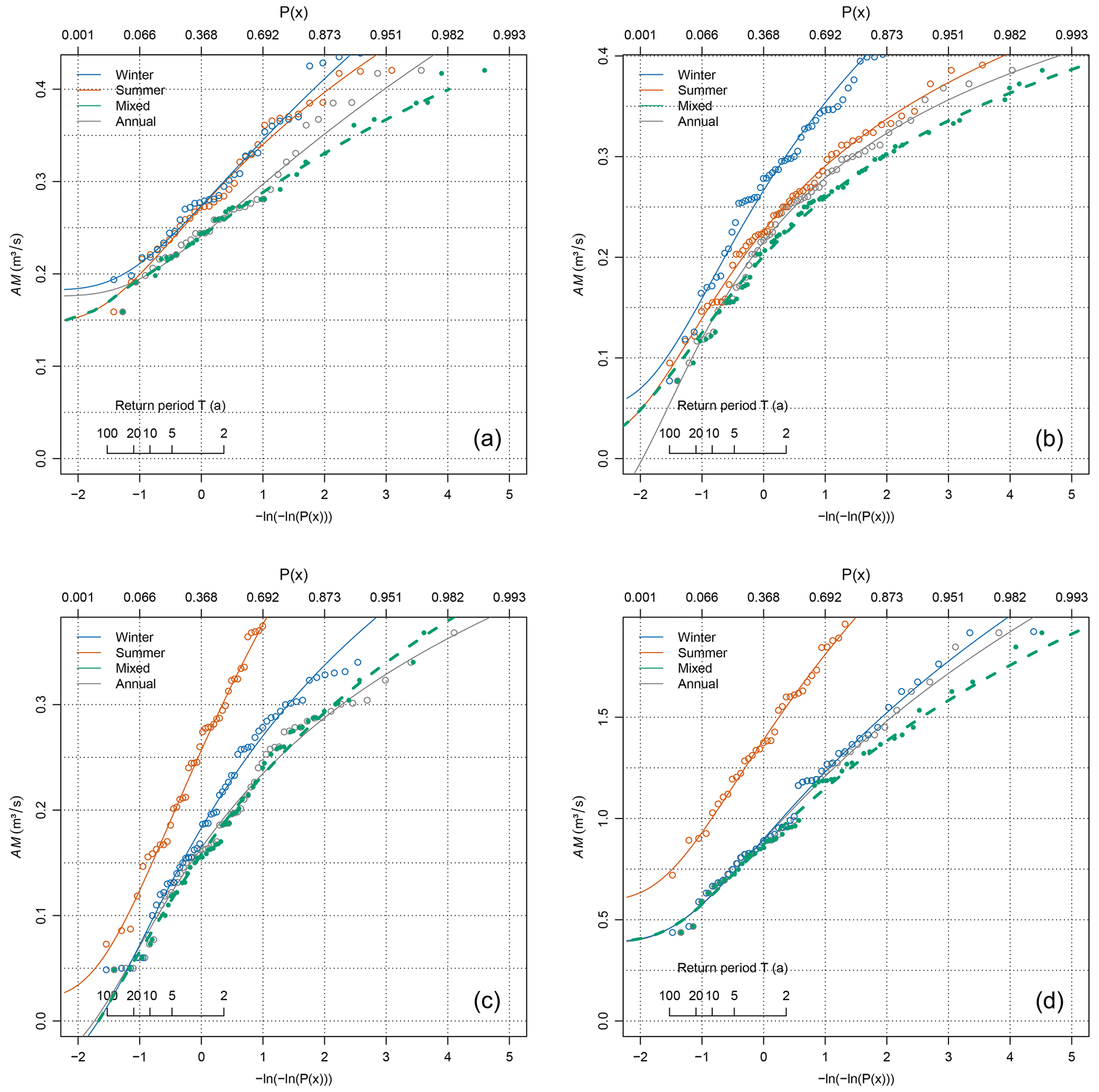
Figure 1Probability plots of summer (red), winter (blue), annual (black), and mixed (green) distributions for archetypal cases. (a) Gauge Ebensee at river Langbathbach situated in the northern foothills of the Alps of Upper Austria; (b) gauge Weg at river Isen situated in low, hilly terrain in Bavaria, Germany; (c) gauge Schönenbach at river Subersach representing an alpine catchment of the Bregenzerwald in Vorarlberg, Austria; and (d) gauge St. Peter-Freienstein at river Vordernberger Bach representing an inner-alpine catchment in Styria, Austria.
Figure 1b gives another example of a highly mixed low-flow regime, albeit with slightly different behaviour. The example is gauge Weg at river Isen situated in low, hilly terrain in Bavaria, Germany. Now 67 % (MR) of annual low flows occur in summer, and the magnitude of summer low flow is somewhat lower (−10 % on average) than the winter low flow. This is indicated by its SR of 0.9. As can be seen from the graph, the summer distribution is always lower than the winter distribution, and only summer low flows occur at the lowest part. The mixed distribution reflects this behaviour by following the summer distribution at the lower tail and combining the probabilities in the range of discharges where low flows in both seasons can occur. In such a case the mixed distribution is always different to the conventional annual distribution and is expected to lead to different results at all probabilities. Notably at high return periods (T>20 years), the mixed probability estimator yields much higher discharge quantiles than the annual probability estimator.
The third example (Fig. 1c) is an alpine catchment in the Bregenzerwald in Vorarlberg, Austria, which again has a lower mixture rate (28 %) and a stronger seasonality (SR=2.41). This is also reflected in a larger gap between the summer and winter distributions, indicating a relatively low probability of low-flow events in summer compared to winter. Consequently, summer low flows should have little effect on mixing probabilities (Eq. 4), and so there should be little difference between the annual and mixed probability estimators. This assumption is also supported by the data example (Fig. 1c). The annual, mixed, and winter distributions coincide in the lower part of the distribution, reflecting moderate to severe low-flow events. For the upper part (high magnitudes) summer low flows can occur but are less likely than winter events. This leads to a slight divergence between the mixed and the annual distribution, although with little significance for the extreme value analysis.
The fourth and final example (Fig. 1d) is an inner-alpine catchment in Styria, Austria, which has the lowest mixture rate (MR=0.11) and again a pronounced seasonality (SR=1.72). Here five summer low-flow events (between 0.90 m3 s−1 for the year 2003 and 1.53 m3 s−1 for the year 1976) mix in the annual minima series and should have little effect on the distribution. Figure 1d shows that the mixed distribution in the data example does indeed completely match the annual distribution for the most interesting area for analysis. Slight divergence occurs only above 0.90 m3 s−1, where the summer low flows are mixed in.
The examples suggest that the mixed model is a valid generalization of the annual probability, since both models coincide for cases when no mixture occurs. In the case of mixed series the annual probability model suffers from a violation of the basic homogeneity assumption, and the mixed model should be used. The examples shed light on the errors that we need to expect from the conventional extreme value statistics in a qualitative way. Below, we assess these errors quantitatively.
3.1 Data set
The mixture model is evaluated based on a comprehensive Austrian data set of natural-like catchments with no or little anthropogenic disturbance to the low-flow regime. The data set has already been used in a number of low-flow studies, addressing seasonality indices (Laaha and Blöschl, 2006b), catchment classification and regional regression (Laaha and Blöschl, 2006), geostatistical methods (Laaha et al., 2014), estimation methods from short records and spot gauging (Laaha and Blöschl, 2005), the link between meteorological drought indices and streamflow (Haslinger et al., 2014), and climate change (Laaha et al., 2016; Parajka et al., 2016; Karanitsch-Ackerl et al., 2019). Most recently, an updated version of the data set has been used for evaluating statistical learning methods (Laimighofer et al., 2022b) and statistical space–time models for low flow (Laimighofer et al., 2022a). In this study we use the data set of Laaha et al. (2016), consisting of 329 Austrian stream gauges with measurements from the 1976 to 2010 period (Fig. 2). The data set includes 312 series with complete records and an additional 17 series with a record of at least 30 years. The data cover catchments from 7 to 7000 km2 with elevations from 159 to 3770 m a.s.l. The mean annual low-flow discharges of these catchments range from 0.03 to 1013 m3 s−1.
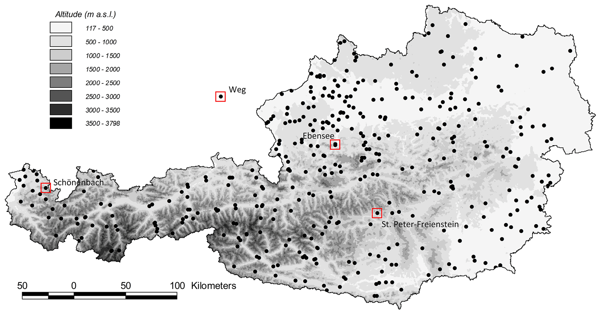
Figure 2Topography and stream gauging network in Austria. Points indicate the location of the 329 gauges used in this study. Example gauges of Fig. 1 are indicated by red squares. Redrawn from Laaha and Blöschl (2006b).
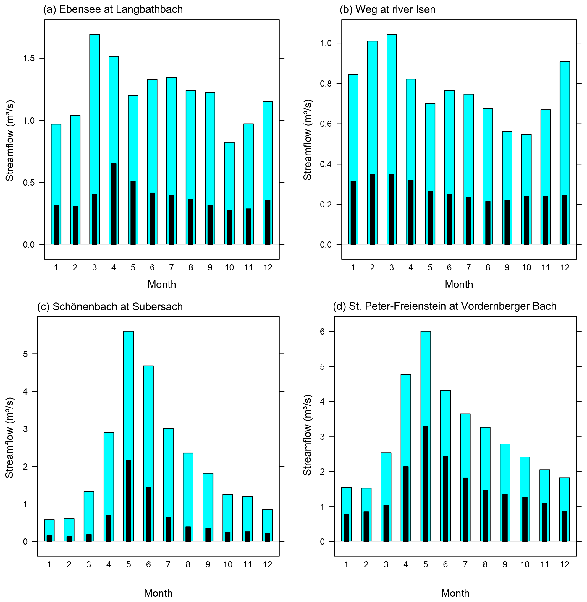
Austria covers an area of 84 000 km2 and is climatically, physiographically, and hydrologically highly diverse. This diversity leads to different low-flow regimes, as illustrated by the monthly hydrographs of the example gauges in Fig. 3. Catchments situated in the forelands and pre-Alps have a rain-dominated regime whose variability is strongly modulated by sustained baseflow at the Weg and Ebensee gauges. Alpine catchments show a snow-dominated regime that is quite pronounced for the Schönenbach and St. Peter-Freienstein gauges. Overall, the low flows in the eastern lowlands occur mainly in summer and are the result of a seasonal water balance deficit triggering stream flow recessions. In the alpine areas in the central and western part of Austria, low flows mainly occur in the winter and are a result of snow storage and frost processes. Both areas are characterized either by a pronounced summer or winter seasonality, with mixture zones of weak seasonality in between. The study area has a very high gauging density and also a high data quality, therefore providing an ideal test bed for the performance of the mixed seasonality estimator.
3.2 Assessment method
3.2.1 Performance measures
The very goal of frequency analysis is to characterize the severity of an event q by its occurrence probability pq or, equivalently, its return period . When we use a different probability model the return period of an event will change, so we are interested in the change of characteristic return periods between the two models. The difference between one model estimate and the other model estimate is referred to in statistics as deviation. When we can assume that one model is superior to the other, the change in performance of the superior model compared to the inferior model can be termed the gain in accuracy. When we place the emphasis on the inferior model, the same quantity can be called an error or loss in accuracy. Note that the interpretation of the deviation as a gain depends on the (reasonable) assumption that the model is superior to the alternative model, and the terminology of the study should be interpreted as such.
Based on this concept, the evaluation of the performance gain at a station of using the mixed probability estimator over the annual probability estimator proceeds in four steps:
-
define the return period of interest (e.g. T=20, 50, 100 years),
-
calculate the associated flow quantile qT of the annual distribution model (using the inverse of its distribution, known as quantile function),
-
insert the value so obtained into the mixed distribution model (Eq. 9) to calculate its probability pmix, and
-
transform the obtained probability into the return period Tmix, which constitutes the improved estimate.
From the assumed input and the obtained output return periods, common deviation statistics are computed. The change of the return period (d) at a station is simply calculated as
It can be expressed as a relative deviation (rd), which makes the measure comparable for different return periods:
The performance gain of a model is finally assessed based on the absolutes of the relative deviation (rad) which is calculated as
3.2.2 Effect of seasonality
The purpose of the mixed probability estimator is to enhance frequency analysis for mixed summer and winter regimes. Its use is based on the assumption that the annual probability estimator suffers from heterogeneity in mixed low-flow regimes, and the mixed seasonality estimator will improve the calculations. Thus, to prove the concept, we test whether, and to what extent, the performance gain of the mixed seasonality estimator depends on seasonality.
In the first step, we assess the strength of the relationship with common low-flow seasonality indices (Laaha and Blöschl, 2006b). This is done by correlation analysis using Pearson and Spearman correlation coefficients. Since the percentage gains have a skewed distribution, we consider both their untransformed and log-transformed values for the analysis. The considered seasonality indices include the variability measure of the circular seasonality index (r) and the seasonality ratio (SR). The SR shows a particular distribution that is symmetric around one (no seasonality) and has decreasing frequency towards the tails of the distribution. We therefore examine the untransformed values and the absolutes of the log-transformed values of SR to test possible linearizations. The circular seasonality measure r has no particular distribution and enters the correlation analysis with untransformed values. The correlation coefficients are tested using standard t-tests with a significance level of α=0.05.
In the second step, we model the dependency of the performance gain from seasonality using linear regression. Since we expect log-linear relationships, we linearize the equations to estimate linear models that fit the particular variables. The models considered are of the following forms:
where y is the relative deviation (rdT) and x the seasonality measure under consideration (r or SR). The symbol ∼ in our notation corresponds to the formula syntax of the statistical software R and is used to specify the relationship between predictand and predictor.
In a final assessment, we evaluate the spatial cross-correlation of the gain in performance with seasonality patterns in Austria from Laaha and Blöschl (2006b). This will shed light under what hydrological conditions the mixed estimator is expected to improve the estimates.
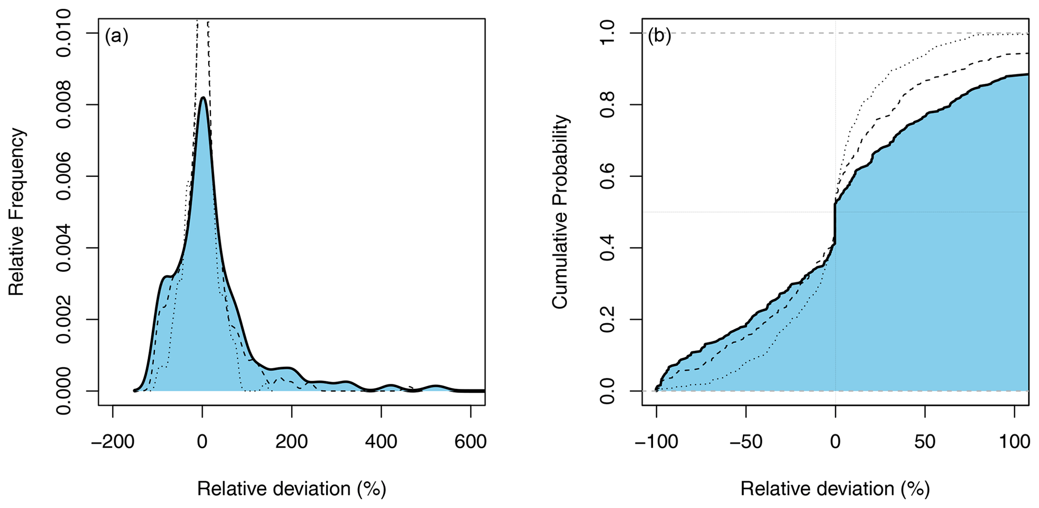
Figure 4Uncertainty of the annual probability estimator as compared to the mixed probability estimator. Shown are the empirical probability density (a) and the cumulative probability (b). Full line with shaded blue area refers to the 100-year event. For comparison the 50-year event (dashed line) and the 20-year event (dotted line) are shown.
4.1 Performance gain of the mixed probability estimator
The deviation distribution of the annual probability estimator as compared to the mixed probability estimator is presented in Fig. 4, and summary statistics are presented in Tables 1 and 2. The results show a very wide dispersion, indicating that the differences between models are large. This applies to all return periods considered, but some variation can be seen. The deviations are most pronounced for the 100-year return period and decrease for 50- and 20-year events, as one would expect.
Table 1Relative absolute deviation (radT) between the annual and mixed probability estimator (%). Q1 and Q3 are the lower and upper quartiles.
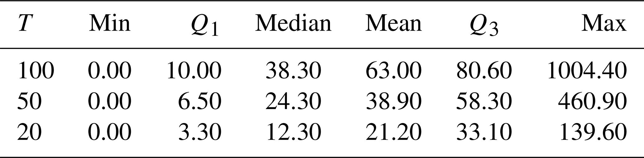
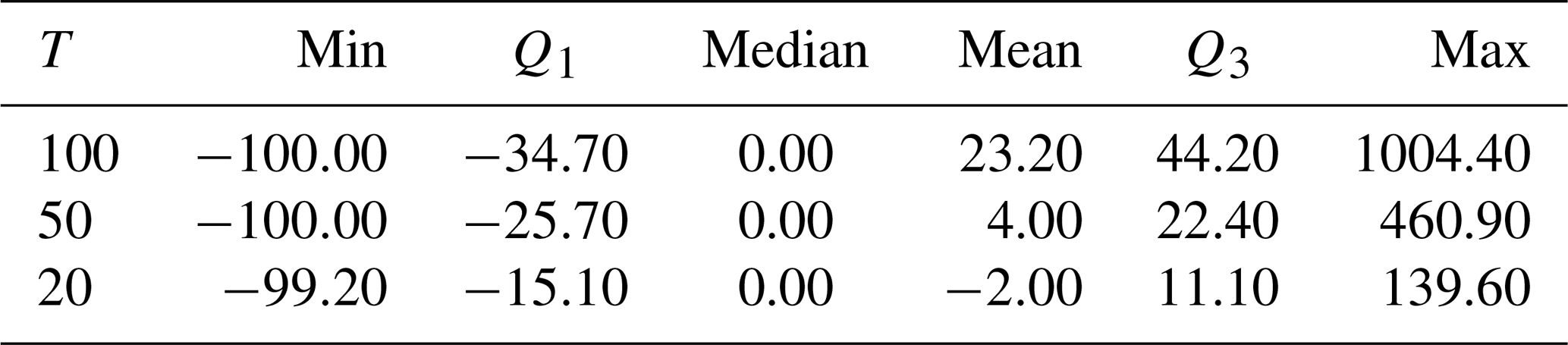
Table 2Relative deviation rdT between the annual and mixed probability estimator (%).
A surprising aspect of the broad distribution is that there must be a large portion of catchments where the mixed distribution approach improves performance. In fact, there are only 32 to 34 (about 10 %) out of a total of 329 cases where the deviation between the models is zero, so using the improved estimator has no effect. These refer to the strongly seasonal cases where the mixed model is based on a single season so that the mixed and annual models coincide (Fig. 1d). For the 100-year event, 75 % of stations (lower quartile Q1) show an (absolute) performance gain of >10 %, 41 % of stations > 50 %, and 25 % of stations (upper quartile Q3) > 80.6 (Table 1). This suggests that the mixed distribution approach is not only relevant in cases with a highly mixed low-flow regime but also applies to catchments with a rather strong seasonal low-flow regime.
More details can be seen from Table 2. The results show a range of accuracy gains from −100 % to +1000 %, with a lower quartile of −35 % and an upper quartile of +44 % for the 100-year event. For the lower return periods, the lower and upper quartiles are −100 % and +461 % for T=50 and −99 % and +140 % for T=20 years. The expected value of the deviations is close to zero for the 20- and 50-year events, indicating that the annual estimator has no systematic bias compared to the mixed estimator for the lower and intermediate return periods. However, for the 100-year events, the expected deviation is +23 %, indicating a substantial overestimation of the return period by the annual estimator.
The effects of using the mixed estimator are most apparent when considering the absolute magnitude of the deviations (Table 1). These make evident that the mixed estimator results in average performance gains of 21 %, 39 %, and 63 % in estimating low flows with T=20, 50-, and 100-year return periods, respectively. Overall, the performance gain is much higher and affects a much larger number of cases than we have expected.
Table 3Correlation of relative absolute deviation (radT) and its logarithm (log (radT)) with seasonality indices r, SR, . All correlations are significant at the α=0.05 level.
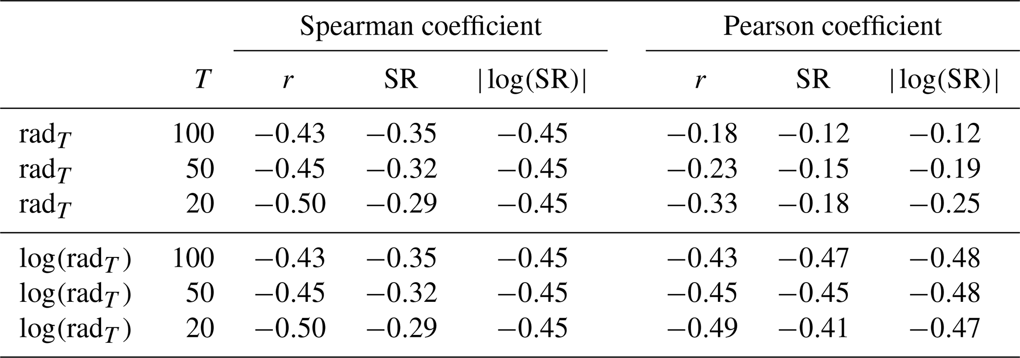
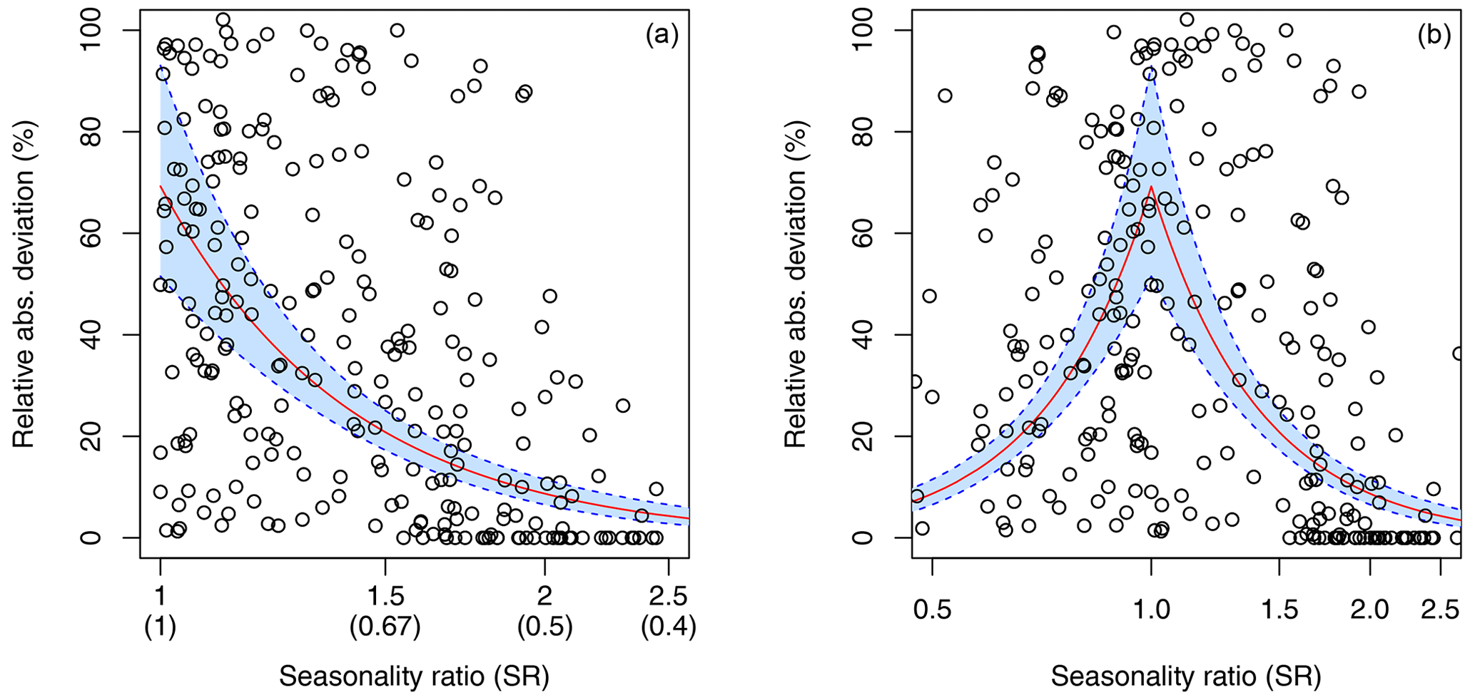
Figure 5Performance gain by seasonality ratio (SR). Shown is the log-linear model between relative absolute deviation (radT) and absolute logs of SR (red lines refer to the expected values, blue to their 95 % confidence bounds). Black points are the observations. In panel (a) SR<1 are plotted as inverted values () and labelled by the numbers in parentheses. Panel (b) plots the same relationship for the original values of SR.
4.2 Effect of seasonality on performance gain
4.2.1 Correlation with seasonality indices
We first assess the strength of the relationship of the accuracy gain with three seasonality indices: the variability measure of the circular seasonality index (mean resultant r), the seasonality ratio SR, and its absolute logarithm . The Spearman and Pearson correlation coefficients are shown in Table 3. All correlations are significant at the α=0.05 level. The strongest relationships can be found for the log-transformed relative absolute deviation. It is, overall, best correlated with the transformed vales of the seasonality ratio, , according to both the Spearman and Pearson coefficients. For the Pearson coefficients the relationships are much stronger for the log transformed than for the untransformed relative absolute deviation. This points to log-linear relationships that can be linearized using a log transformation. Here, the untransformed abs(SR) reaches almost the same correlation as , and the correlation of r is only slightly lower. For the Spearman coefficients the results are insensitive for a log transformation of the relative absolute deviation. Overall the performance gain of the mixed estimator is strongly correlated with seasonality, and a log transformation can help linearize the relationship.
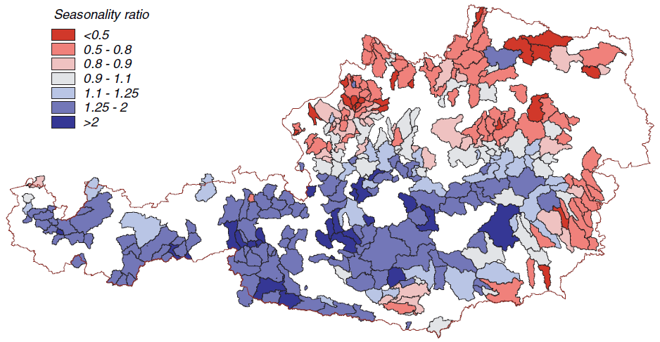
Figure 6Ratio of summer and winter low-flow discharges (SR) for 325 subcatchments in Austria. SR>1 indicates a winter low-flow regime, and SR<1 indicates a summer low-flow regime. From Laaha and Blöschl (2006b).
4.2.2 Expected performance gain by seasonality
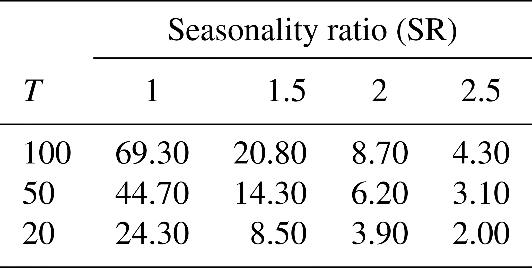
As the second step of the analysis we model the dependency of the performance gain from seasonality using log-linear regression (Fig. 5). Despite the large variability in the data, the regression model appears to be well suited, because it is able to represent the decrease in variability with increasing seasonality. Table 4 shows the expected gains from the regression model for various return periods. For the 100-year event, the expected gain is about 70 % for SR=1.0, 20 % for SR=1.5, and 10 % for SR=2.0. For the 50-year event the expected gain is about two-thirds as large, and for the 20-year event the gain is almost half as large. The results show that the gain of using the mixed probability estimator is not only limited to highly mixed regimes but also applies to strongly seasonal ones. The gain is particular large for high return periods where results are expected to differ strongly for a wide range of regimes. For low return periods such as T=20 years, strong effects can be found for highly mixed regimes (say, SR<1.5), whereas there is little gain for highly seasonal regimes.
Table 4Expected performance gain (%) from the regression model for various return periods.
4.2.3 Spatial cross-correlation with seasonality patterns in Austria
In the final step of the analysis, the relative absolute deviations are compared with the spatial patterns of SR in the study area to shed light on the hydrological and topographic relevance of the mixed probability estimator. Figure 6 from Laaha and Blöschl (2006b) presents a map of the seasonality index SR. The patterns correlate strongly with the topography of the study area, with strong winter seasonality in the high Alps, strong summer seasonality in the lowlands, and mixed regimes in between. Figure 7 shows the relative gain by seasonality ratio using the same classes as used in the map. The lowest gains can be observed for strong winter seasonality (SR>2) where the mixed estimator is almost identical with the annual estimator. For all other classes the differences are substantial, having an expected value of at least 25 %. Importantly, this also includes the highly summer dominated catchments where one would expect the annual estimator to be well suited. This is because in cold temperate climate, low-flow relevant frost events can also occur in the lower catchments in some years, which are then mixed in the annual low-flow distribution. The highest gain is observed for mild summer low-flow regimes (SR between 1.1 and 1.25) which correspond to typical mid-mountain catchments where the frost events are enhanced by the slightly higher altitude, and the mixture between summer and winter events is particularly strong. The results suggest that the mixed estimator is relevant not only for catchments in mountainous regions but also for most catchments, except for the high alpine ones.
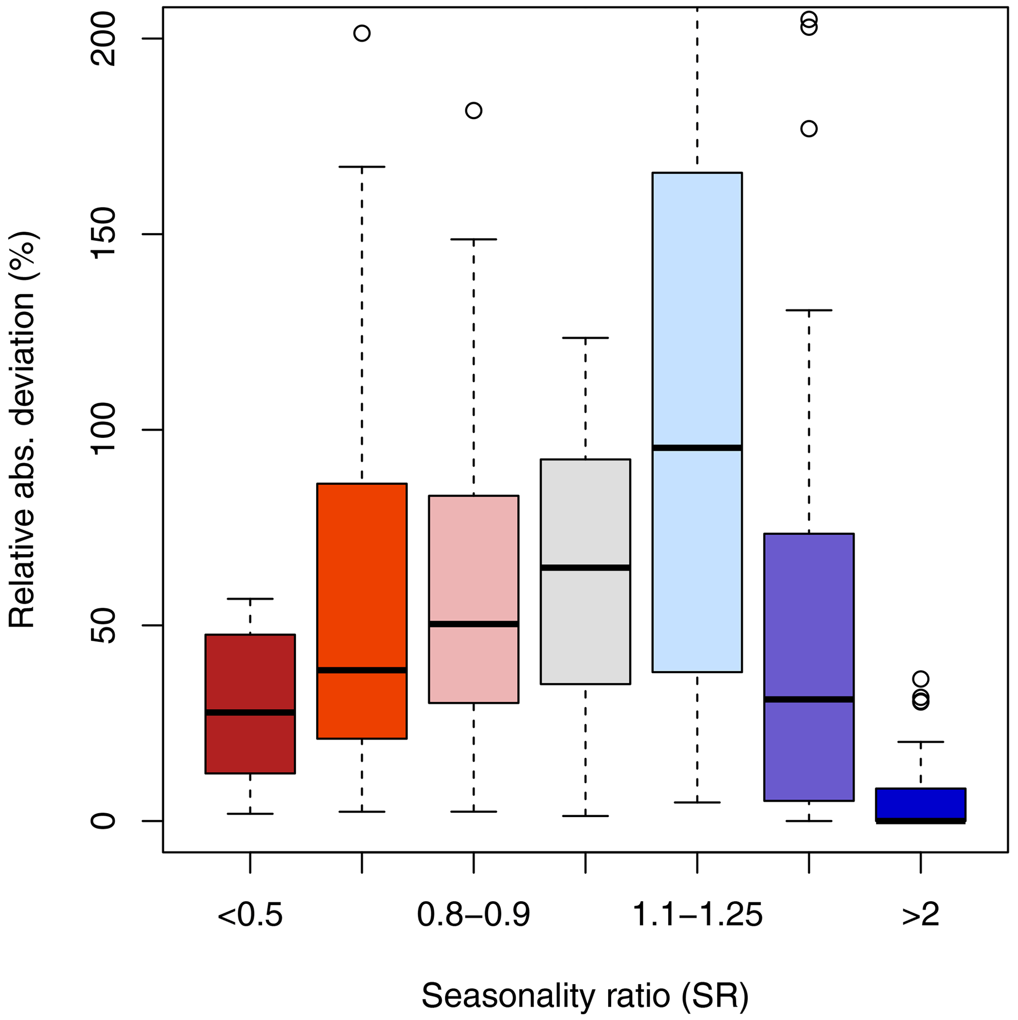
Figure 7Performance gain by seasonality ratio classes of Laaha and Blöschl (2006b). Shown are the relative absolute deviations (radT) for the T = 100-year event. The colour coding is that of Fig. 6.
This paper proposes a mixed distribution approach to perform frequency analysis in catchments with mixed summer and winter low-flow regimes. We formulated the theoretical basis of the mixed distribution approach for the lower extremes based on annual minima series. The performance of the model was evaluated based on a comprehensive Austrian data set. Results indicate that the model performs well for a range of low-flow regimes, from distinct winter and summer regimes to mixed regimes where seasonal occurrence in summer and winter is equally likely. This finding goes far beyond our expectation that the mixed estimator would be relevant only for highly mixed regimes and that its application would be limited mainly to mountain forelands. On average, for the study area, the deviation is reduced by 21 %, 39 %, and 63 % when the low flow with a return period of 20, 50, and 100 years is estimated, respectively.
The performance gain depends on the degree of mixture, or the seasonality ratio, as one would expect. For the 100-year event, the expected gain is about 70 % for SR=1.0, 20 % for SR=1.5, and 10 % for SR=2.0. For the 50-year event the expected gain is about two-thirds as large, and for the 20-year event the gain is almost half as large. The gain is substantial for high return periods where results are expected to differ strongly for nearly all seasonal regimes. For low return periods such as T=20 years, strong effects can be found for highly mixed regimes (say, SR<1.5), whereas the gain for strongly seasonal regimes is quite low.
As illustrated by archetypal examples, the mixed estimator has very favourable properties: if no mixture occurs, both approaches provide the same results. This means that the mixed estimator is a valid generalization of the common annual estimator. If mixture occurs, the seasonally differentiated statistics can better take it into account. The mixed distribution approach is therefore a more efficient estimator for seasonally mixed low-flow series. An additional strength of the model is that it allows the user to estimate return periods of summer low flows, winter low flows, and annual return periods in a theoretically sound and consistent manner, resulting in coherent seasonal and annual statistics. This supports the estimates of seasonal statistics that are increasingly needed, such as for assessing environmental flows or hydropower production capacity.
Similar advantages of the mixed seasonality estimator have been found for high flows, such as by Schumann (2005) when assessing the extreme 2005 event at the Mulde River basin in Germany. The study also found the seasonal statistics more robust with respect to single extreme values than statistics based on annual values. The same effect can be seen from our example in Fig. 1b, where the annual statistic largely underestimates the magnitude of extreme events. The mixed distribution, however, coincides with the seasonal distributions in an intuitive way, and thus offers the plausible estimator in such a case.
Despite there being a high degree of similarity between flood and low-flow applications, some important differences exist. Fischer et al. (2016) noted that distinguishing between summer and winter floods is not always as easy when seasonal series contain events with different genesis. Indeed, the published examples of mixed flood distributions (e.g. Deutsche Vereinigung fúr Wasserwirtschaft, 2012) are less clear, as they do not show a similar clear separation between the seasonal distributions as the examples for low flow in our paper (Fig. 1). Floods are generated by a wide range of process combinations (Merz and Blöschl, 2003) that are not confined to a season to the same extent as low-flow events. This leads to some limitation of seasonal flood statistics, or in other words, makes seasonal low-flow statistics even more relevant. As a remedy, Fischer et al. (2016) proposed to further subdivide summer floods into groups of long and short events based on their time scale to improve the separation of processes. However, they had to consider overlapping events, because the events they identified were not independent anymore.
Although the distinction between summer and winter low-flow events is more straightforward, the assumption of their seasonal independence is a strong one that is unlikely to be met in a number of catchments. Baseflow has a long persistence along with the climate drivers that generate hydrological drought, giving potential for strong temporal autocorrelation. This may for example occur in large watersheds with a high storage capacity and, therefore, a particularly long time of recession and recovery at the end of the drought. To what extent the assumption of seasonal independence is fulfilled can be inferred from the correlation between summer and winter events. In the case of the Austrian study area, two thirds of the catchments show a highly significant seasonal correlation (46 % at the α=0.01 level) or significant seasonal correlation (22 % at the α=0.05 level) when using the Spearman coefficient as a reference. Such correlation may be evidence of the occurrence of rain-to-snow season droughts (Van Loon et al., 2015) or simply that the watershed has not fully recovered from the summer event when the winter event occurs. Both will have an effect on the mixture of distributions. We therefore see that the estimator could be further improved by taking into account the correlation structure of the events, which would be a valuable extension of the method for cases where seasonal correlations occur. Such an approach appears to be a natural extension of the mixed probability estimator and will be explored in the companion paper to this study (Laaha, 2022).
Apart from this limitation, the mixed distribution approach provides one consistent approach for summer, winter, and annual events that is more accurate than the traditional annual minima estimator. Because of all its beneficial properties, it should be used in the analysis of low-flow frequencies in climates with warm summer and cold winter seasons, under conditions where mixed seasonal low-flow regimes occur.
The code will be made available in an updated version of the R software package “lfstat” via the CRAN repository (https://CRAN.R-project.org/package=lfstat; Gauster et al., 2022).
Data can be made available on personal request to gregor.laaha@boku.ac.at.
The author has declared that there are no competing interests.
Publisher's note: Copernicus Publications remains neutral with regard to jurisdictional claims in published maps and institutional affiliations.
Data provision by the Hydrographical Service of Austria (HZB) is highly appreciated. This research is a contribution to the UNESCO IHP VIII FRIEND-Water programme. We would like to thank the editor and two reviewers for their valuable comments on the manuscript.
This research has been supported by the Climate and Energy Fund under the programme “ACRP” (grant no. C265154).
This paper was edited by Lelys Bravo de Guenni and reviewed by two anonymous referees.
Coles, S.: An introduction to statistical modeling of extreme values, in: Springer series in statistics, Springer, London, New York, ISBN 978-1-85233-459-8, 2001. a
Deutsche Vereinigung für Wasserwirtschaft (Ed.): Ermittlung von Hochwasserwahrscheinlichkeiten, no. M 552 in DWA-Regelwerk, August 2012 Edn., oCLC: 809196700, DWA, Hennef, ISBN 978-1-85233-459-8, 2012. a, b
Fischer, S., Schumann, A., and Schulte, M.: Characterisation of seasonal flood types according to timescales in mixed probability distributions, J. Hydrol., 539, 38–56, https://doi.org/10.1016/j.jhydrol.2016.05.005, 2016. a, b
Gauster, T., Laaha, G., and Koffler, D.: lfstat – calculation of low flow statistics for daily stream flow data, R package version 0.9.12, CRAN [code], https://CRAN.R-project.org/package=lfstat, last access: 8 November 2022. a
Gumbel, E. J.: Distributions des valeurs extremes en plusiers dimensions, Publ. Inst. Statist. Univ., Paris, 9, 171–173, 1960. a
Haslinger, K., Koffler, D., Schöner, W., and Laaha, G.: Exploring the link between meteorological drought and streamflow: Effects of climate-catchment interaction, Water Resour. Res., 50, 2468–2487, https://doi.org/10.1002/2013WR015051, 2014. a
Karanitsch-Ackerl, S., Mayer, K., Gauster, T., Laaha, G., Holawe, F., Wimmer, R., and Grabner, M.: A 400-year reconstruction of spring–summer precipitation and summer low flow from regional tree-ring chronologies in North-Eastern Austria, J. Hydrol., 577, 123986, https://doi.org/10.1016/j.jhydrol.2019.123986, 2019. a
Laaha, G.: A mixed distribution approach for low-flow frequency analysis – Part 2: Modeling dependency using a copula-based estimator, Hydrol. Earth Syst. Sci. Discuss. [preprint], https://doi.org/10.5194/hess-2022-358, in review, 2022. a, b, c
Laaha, G. and Blöschl, G.: Low flow estimates from short stream flow records – a comparison of methods, J. Hydrol., 306, 264–286, https://doi.org/10.1016/j.jhydrol.2004.09.012, 2005. a
Laaha, G. and Blöschl, G.: A comparison of low flow regionalisation methods–catchment grouping, J. Hydrol., 323, 193–214, https://doi.org/10.1016/j.jhydrol.2005.09.001, 2006a. a
Laaha, G. and Blöschl, G.: Seasonality indices for regionalizing low flows, Hydrol. Process., 20, 3851–3878, https://doi.org/10.1002/hyp.6161, 2006b. a, b, c, d, e, f, g, h, i
Laaha, G., Skøien, J., and Blöschl, G.: Spatial prediction on river networks: comparison of top-kriging with regional regression, Hydrol. Process., 28, 315–324, https://doi.org/10.1002/hyp.9578, 00000, 2014. a
Laaha, G., Parajka, J., Viglione, A., Koffler, D., Haslinger, K., Schöner, W., Zehetgruber, J., and Blöschl, G.: A three-pillar approach to assessing climate impacts on low flows, Hydrol. Earth Syst. Sci., 20, 3967–3985, https://doi.org/10.5194/hess-20-3967-2016, 2016. a, b
Laaha, G., Gauster, T., Tallaksen, L. M., Vidal, J.-P., Stahl, K., Prudhomme, C., Heudorfer, B., Vlnas, R., Ionita, M., Van Lanen, H. A. J., Adler, M.-J., Caillouet, L., Delus, C., Fendekova, M., Gailliez, S., Hannaford, J., Kingston, D., Van Loon, A. F., Mediero, L., Osuch, M., Romanowicz, R., Sauquet, E., Stagge, J. H., and Wong, W. K.: The European 2015 drought from a hydrological perspective, Hydrol. Earth Syst. Sci., 21, 3001–3024, https://doi.org/10.5194/hess-21-3001-2017, 2017. a
Laimighofer, J., Melcher, M., and Laaha, G.: Low-flow estimation beyond the mean – expectile loss and extreme gradient boosting for spatiotemporal low-flow prediction in Austria, Hydrol. Earth Syst. Sci., 26, 4553–4574, https://doi.org/10.5194/hess-26-4553-2022, 2022a. a
Laimighofer, J., Melcher, M., and Laaha, G.: Parsimonious statistical learning models for low-flow estimation, Hydrol. Earth Syst. Sci., 26, 129–148, https://doi.org/10.5194/hess-26-129-2022, 2022b. a
Merz, R. and Blöschl, G.: A process typology of regional floods, Water Resour. Res., 39, 1340, https://doi.org/10.1029/2002WR001952, 2003. a
Parajka, J., Blaschke, A. P., Blöschl, G., Haslinger, K., Hepp, G., Laaha, G., Schöner, W., Trautvetter, H., Viglione, A., and Zessner, M.: Uncertainty contributions to low-flow projections in Austria, Hydrol. Earth Syst. Sci., 20, 2085–2101, https://doi.org/10.5194/hess-20-2085-2016, 2016. a
Schumann, A.: Hochwasserstatistische Bewertung des Augusthochwassers 2002 im Einzugsgebiet der Mulde unter Anwendung der saisonalen Statistik, Hydrol. Wasserbewirt., 49, 200–206, 2005. a, b
Stedinger, J. R., Vogel, R. M., and Foufoula-Georgiou, E.: Frequency analysis of extreme events, in: Chapter 18 in Handbook of Hydrology, edited by: Maidment, D. R., McGraw-Hill, ISBN 9780070397323, 1993. a, b
Tallaksen, L. M. and Van Lanen, H. A. J.: Hydrological drought: processes and estimation methods for streamflow and groundwater, in: no. 48 in Developments in water science, Elsevier, ISBN 9780444516886, 2004. a
Van Loon, A. F., Ploum, S. W., Parajka, J., Fleig, A. K., Garnier, E., Laaha, G., and Van Lanen, H. A. J.: Hydrological drought types in cold climates: quantitative analysis of causing factors and qualitative survey of impacts, Hydrol. Earth Syst. Sci., 19, 1993–2016, https://doi.org/10.5194/hess-19-1993-2015, 2015. a
Yue, S., Ouarda, T., Bobée, B., Legendre, P., and Bruneau, P.: The Gumbel mixed model for flood frequency analysis, J. Hydrol., 226, 88–100, https://doi.org/10.1016/S0022-1694(99)00168-7, 1999. a