the Creative Commons Attribution 4.0 License.
the Creative Commons Attribution 4.0 License.
 | 01 Feb 2023
Climate sensitivity of the summer runoff of two glacierised Himalayan catchments with contrasting climate
Sourav Laha
Argha Banerjee
Ajit Singh
Parmanand Sharma
Meloth Thamban
The future changes in runoff of Himalayan glacierised catchments will be determined by the local climate forcing and the climate sensitivity of the runoff. Here, we investigate the sensitivity of summer runoff to precipitation and temperature changes in the winter-snow-dominated Chandra (the western Himalaya) and summer-rain-dominated upper Dudhkoshi (the eastern Himalaya) catchments. We analyse the interannual variability of summer runoff in these catchments during 1980–2018 using a semi-distributed glacio–hydrological model, which is calibrated with the available runoff and glacier mass-balance observations. Our results indicate that despite the contrasting precipitation regimes, the catchments have a similar runoff response: the summer runoff from the glacierised parts of both catchments is sensitive to temperature changes and insensitive to precipitation changes; the summer runoff from the non-glacierised parts of the catchments has the exact opposite pattern of sensitivity. The precipitation-independent glacier contribution stabilises the catchment runoff against precipitation variability to some degree. The estimated sensitivities capture the characteristic “peak water” in the long-term mean summer runoff, which is caused by the excess meltwater released by the shrinking ice reserve. As the glacier cover depletes, the summer runoff is expected to become more sensitive to precipitation forcing in these catchments. However, the net impact of the glacier loss on the catchment runoff may not be detectable, given the relatively large interannual runoff variability in these catchments.
- Article
(5074 KB) - Full-text XML
-
Supplement
(1157 KB) - BibTeX
- EndNote


The presence of glaciers in a catchment significantly influences the diurnal to seasonal to interannual variability of the runoff as well as its long-term multidecadal changes (Hock et al., 2005). Himalayan glacier-fed rivers play a key part in sustaining the downstream population and ecosystem (Azam et al., 2021). It is important to analyse the potential catchment-scale hydrological changes in the Himalaya since a significant reduction in the regional glacier cover is expected by 2100 (Kraaijenbrink et al., 2017). This problem has motivated several glacio–hydrological model studies of the Himalayan basins and catchments (see Azam et al., 2021 for a review). These models often differ from each other in the level of descriptions of glacial processes, e.g. no explicit treatment of the glaciers (Pokhrel et al., 2014), a static (Nepal, 2016) or dynamic (Kraaijenbrink et al., 2017) glacier cover, a simple temperature-index model (Chandel and Ghosh, 2021; Banerjee, 2022), or a detailed energy-balance model (Fujita and Sakai, 2014). Even a single model, when tuned with different available baseline climate data products, predicts a wide range of future hydrological changes (Koppes et al., 2015). In addition, the available future climate projections used to drive the glacio–hydrological models have a large spread (Sanjay et al., 2017). All of the above factors contribute to a wide range of predictions for the future changes in the runoff of Himalayan catchments (e.g. Nie et al., 2021). Assessing climate sensitivity of the runoff of Himalayan catchments may prove to be useful in reconciling the range of predictions available in the literature. Climate sensitivity of runoff is defined as the change in runoff due to a unit perturbation in a forcing variable, e.g. precipitation or temperature (Zheng et al., 2009). The climate sensitivities estimated from different models, which are forced by different projected climate forcing, can therefore be compared (Vano et al., 2012). A climate sensitivity analysis may also reveal key differences and similarities in the climate response of runoff generated from the different parts of a catchment (Banerjee, 2022) that are dominated by either snowmelt, glacier melt, or rainfall (Fujita and Sakai, 2014). It may also bring out the similarities and the differences among catchments across the Himalayan arc with their distinct climate settings and, thus, provide a better handle on the runoff response in the ungauged catchments in this data-sparse region (Azam et al., 2021).
In the literature, climate sensitivities have been used to estimate long-term runoff changes due to temperature and precipitation forcing in both glacierised (Chen and Ohmura, 1990) and non-glacierised catchments (Dooge et al., 1999; Zheng et al., 2009; Vano et al., 2012). In the Himalaya, climate sensitivity of glacier mass balance proved to be useful for explaining the observed spatial pattern of glacier thinning (Sakai and Fujita, 2017; Kumar et al., 2019), or for the identification of an inherent bias in scaling-based glacier evolution models which are often used in glacio–hydrological studies (Banerjee et al., 2020). A recent study used a simple temperature-index model to establish a weak precipitation sensitivity of glacier runoff in general (Banerjee, 2022).
Despite its potential utility, detailed studies of the climate sensitivity of the runoff of Himalayan glacierised catchments are limited (Fujita and Sakai, 2014; Azam and Srivastava, 2020). Motivated by this gap, the present study uses a detailed process-based glacio–hydrological model to explore the sensitivity of glacier and off-glacier summer runoff and to analyse the underlying mechanisms driving the sensitivities. Note that throughout the paper, the annual quantities correspond to the hydrological year from 1 October of a calendar year to 30 September of the next, and summer season refers to the period from 1 May to 30 September (e.g. Azam et al., 2019). Also, runoff of a catchment implies the streamflow at the catchment outlet, and glacier (off-glacier) runoff denotes the contribution of the glacierised (glacier-free) areas of the catchment to the streamflow. We study two contrasting glacierised Himalayan catchments: winter-precipitation-dominated Chandra (the western Himalaya) and summer-precipitation-dominated upper Dudhkoshi (the eastern Himalaya). Climate sensitivities of runoff can be obtained by simply regressing the observed variability of runoff to those of its meteorological drivers (e.g. Zheng et al., 2009). When observations are not available, model simulations can be used for the same (Vano et al., 2012). Here, we use the variable infiltration capacity (VIC) model (Liang et al., 1996), augmented with a glacier-melt module, to simulate runoff of the studied catchment over the period 1980–2018. The simulated runoff is used to estimate and validate the sensitivities of summer runoff to annual precipitation and summer temperature. The sensitivities of the runoff of the glacierised and non-glacierised parts of the catchments are also analysed separately. These sensitivities are then used to understand the multidecadal changes in the mean and the variability of summer runoff of the two catchments as the glaciers shrink in a warming climate.
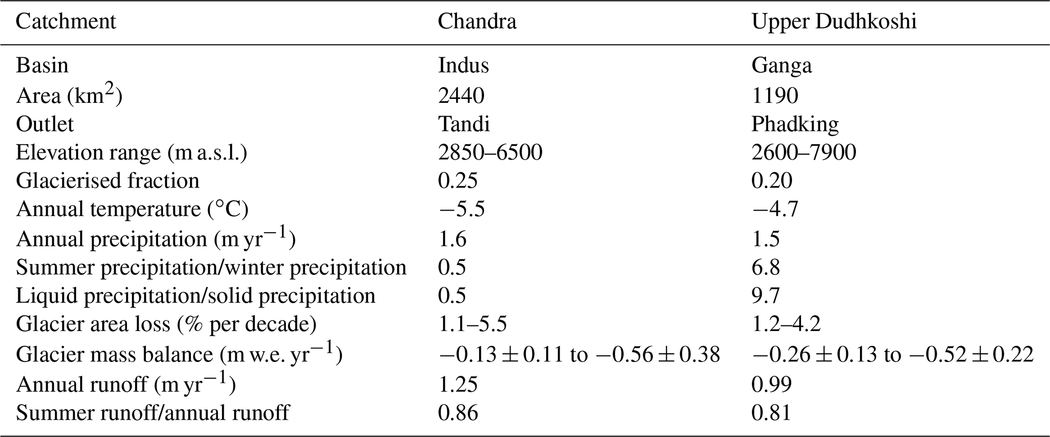
We considered two high Himalayan catchments with contrasting climate regimes: Chandra (Indus basin, the western Himalaya) and upper Dudhkoshi (Ganga basin, the eastern Himalaya) (Figs. 1 and 2). The Chandra catchment is in the Lahaul–Spiti district, Himachal Pradesh, India. The upper Dudhkoshi catchment is located in the Solukhumbu district of Nepal. The mean annual precipitation is similar in both catchments, but its seasonality is different. About 70 % of the annual precipitation in the Chandra catchment occurs during the winter months (Fig. 1c) due to the western disturbances (Azam et al., 2019), and the influence of the Indian summer monsoon is relatively weak. In the upper Dushkoshi catchment, more than 80 % of the precipitation happens during the summer months (Fig. 1c) with a dominant influence of the Indian summer monsoon. Consequently, glacier accumulation mainly occurs during winter (summer) months in the Chandra (upper Dudhkoshi) catchment. Due to the contrasting seasonality of precipitation, the ratio of liquid to solid precipitation in the Chandra and upper Dudhkoshi catchments are 0.5 and 9.7, respectively (Table 1). The catchment area of upper Dudhkoshi is approximately half of the Chandra catchment. The glacierised fraction in the Chandra catchment is 20 % higher than that of upper Dudhkoshi. The mean annual temperature is 0.8 ∘C lower in the Chandra catchment compared to the upper Dudhkoshi catchment. However, the former has a more pronounced seasonality with a warmer summer and a cooler winter (Fig. 1d). The Chandra catchment has a somewhat higher annual and summer runoff. Some important characteristics of the two catchments are compared in Table 1.
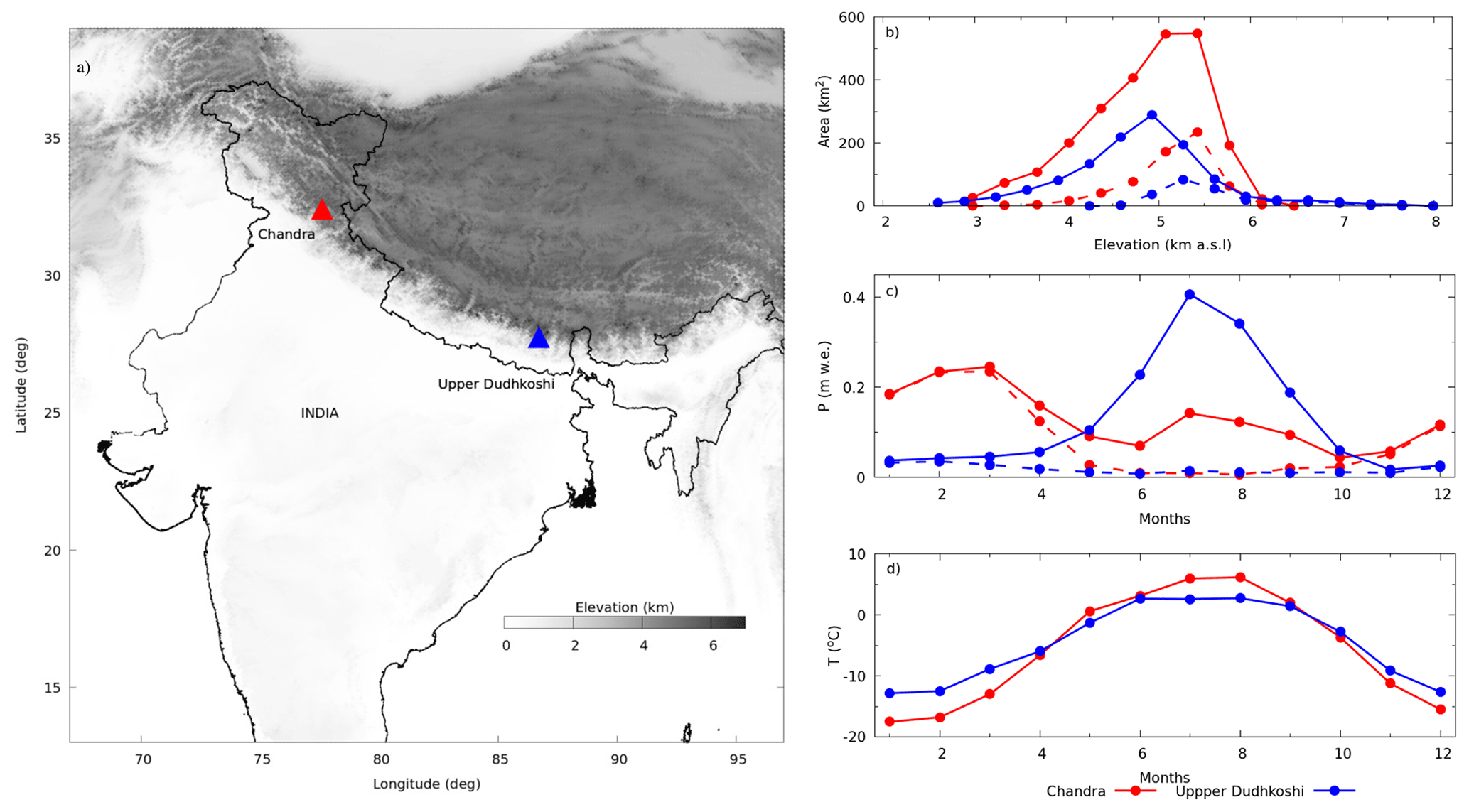
Figure 1(a) The location of the Chandra (solid red triangle) and upper Dudhkoshi (solid blue triangle) catchments on a grey-scale elevation map (Amante and Eakins, 2009). In the rest of the plots, red (blue) colours refer to the Chandra (upper Dudhkoshi) catchment. The solid magenta (sky-blue) polygon shows Ganga (Indus) basin. (b) Area–elevation distribution of the catchments (solid lines + solid symbols) and that of the glacierised parts (dashed lines + solid symbols). (c) Mean monthly precipitation (solid lines + solid symbols), along with the monthly snowfall (dashed lines + solid symbols). (d) Mean monthly temperature profiles (solid lines + solid symbols).
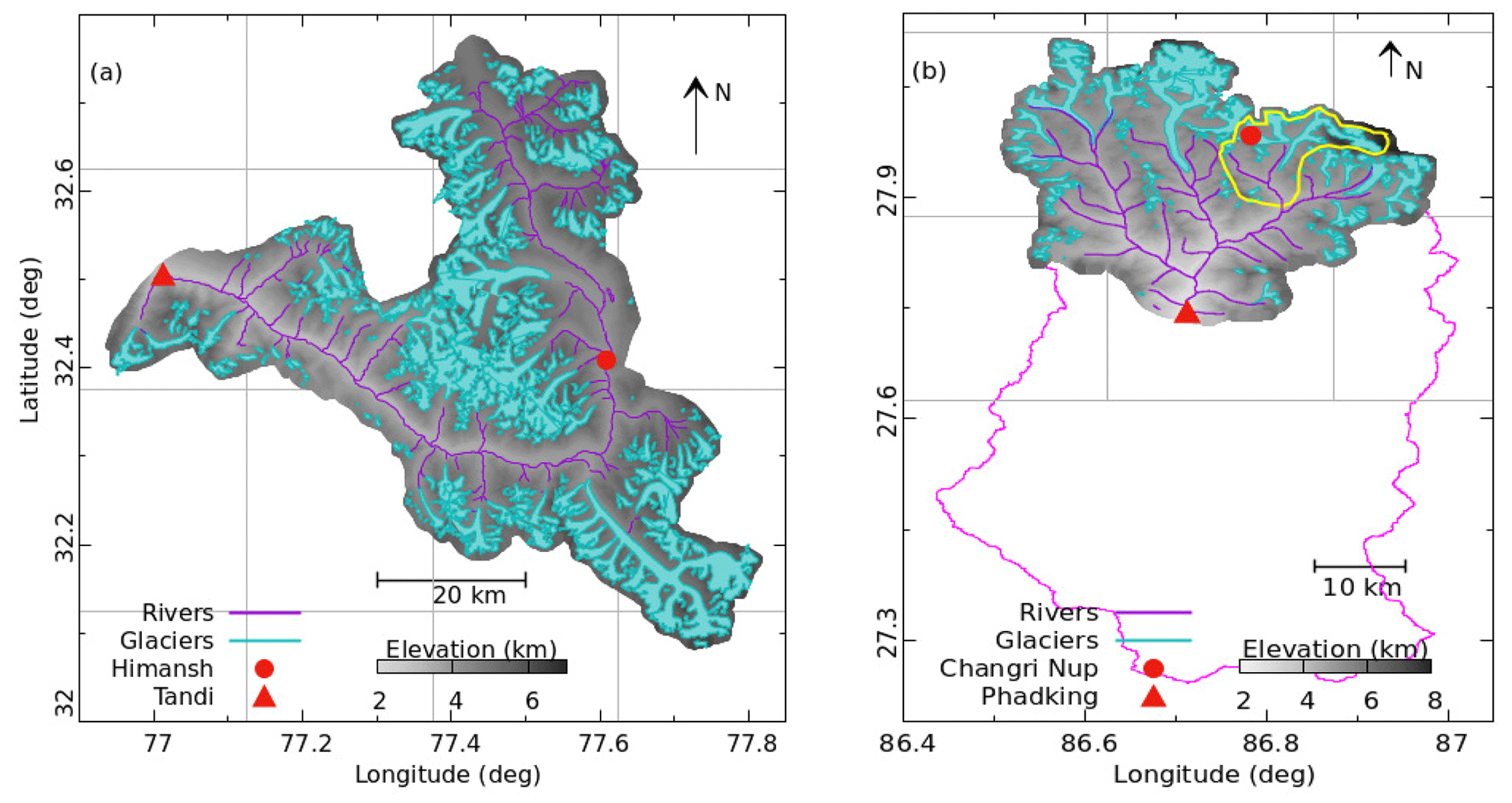
Figure 2Maps of (a) Chandra and (b) upper Dudhkoshi catchments showing glaciers (cyan polygons) and streams (purple lines). The solid red circles (triangles) are the meteorological (hydrological) stations. The ERA5 grid boxes are shown with solid grey lines in the background. Solid magenta and yellow polygons show Dudhkoshi and Periche catchments.
Table 1A summary of the characteristics of the Chandra and upper Dudhkoshi catchments. The meteorological variables are bias-corrected reanalysis data averaged over the catchments (Hersbach et al., 2020), the hydrological data are from model simulations (the present study). The glacier mass-balance and area-loss estimates are from the existing literature (Table S3).
Below we present methodological details related to the input data, the glacio–hydrological model, and the climate sensitivity analysis.
3.1 Hydrometeorological and glaciological data
3.1.1 Observations
Observed hourly runoff of the Chandra river at Tandi (32.55∘ N, 76.97∘ E, 2850 m a.s.l.) from 26 June 2016 to 30 October 2018 was available for three summer seasons with some data gaps (Fig. 5b) (Singh et al., 2020; Table S1 in the Supplement). Hourly 2 m air temperature, precipitation, and incoming short-wave radiation were measured at the Himansh station (32.409∘ N, 77.609∘ E, 4080 m a.s.l.) in the catchment between 18 October 2015 to 5 October 2018 with some data gaps (Oulkar et al., 2022, Table S1).
Hourly runoff from upper Dudhkoshi catchment was observed at Phadking (27.74∘ N, 86.71∘ E, 2600 m a.s.l.) between 7 April 2010 and 16 April 2017 (Fig. 5a) (Chevallier et al., 2017). Available hourly air temperature and precipitation data at Phadking from 7 April 2010 to 23 April 2017 (with some data gaps) (Chevallier et al., 2017) were used. The daily incoming short-wave radiation data for the period 1 November 2010 to 30 November 2014 at nearby Changri Nup station (27.983∘ N, 86.783∘ E, 5400 m a.s.l.) in the same catchment were used (Sherpa et al., 2017; Table S1).
We considered eight available geodetic mass-balance observations that spanned a decade or more, for each of the catchments (Table S3). The Randolph Glacier Inventory (RGI 6) (RGI Consortium, 2017) was used for the glacier boundaries that corresponded to the glacier extent in 2002.
3.1.2 Reanalysis data and bias correction
We used hourly 2 m air temperature, precipitation, and wind speed from ERA5, the fifth generation European Centre for Medium-Range Weather Forecast (ECMWF) atmospheric reanalysis of the global climate from 1980 to 2018 (Hersbach et al., 2020), to force the VIC model at a spatial resolution of . Following the existing hydrological studies of various high Himalayan catchments (Soncini et al., 2016; Azam and Srivastava, 2020), the temperature data were bias-corrected. The available observed air-temperature data at the Himansh station (Chandra catchment), and at Phadking (Dudhkoshi catchment) were used to compute the mean monthly temperature biases (Fig. S1 in the Supplement), assumed to be constant for the whole catchment and over the whole simulation period.
To compute temperature at any given elevation within a grid box, mean monthly lapse rates (Fig. S2) were used. In the Chandra catchment, the lapse rates were computed at the grid box containing Himansh station using ERA5 temperature from the four near-neighbour grid boxes. The corresponding annual lapse rate of 4.7±1.2 ∘C km−1 was consistent with previously observed values of 4.4–6.4 ∘C km−1 (Azam et al., 2019; Pratap et al., 2019). In upper Dudhkoshi catchment, the monthly lapse rates derived from ERA5 were significantly larger than those observed between Phadking and Changri Nup stations over the period 2013–2016, so we used the observed lapse rates. The corresponding mean annual lapse rate of 4.6±0.6 ∘C km−1 in this catchment was the same as that previously reported (Pokhrel et al., 2014).
The ERA5 precipitation data were corrected by scaling with a catchment-specific constant αP for each of the catchments following the existing studies from the region (Huss and Hock, 2015; Bhattacharya et al., 2019; Azam and Srivastava, 2020). The scale factor, which ensured water balance over the catchments, was calibrated using the observed runoff and glacier mass balance employing a Bayesian procedure (see Sect. 3.2.3). In some of the existing studies in the region, an elevation-dependent precipitation scaling has also been employed (e.g. Azam et al., 2019). However, as an elevation-dependent correction may potentially introduce additional uncertainties (e.g. Johnson and Rupper, 2020), we preferred a constant αp, keeping the number of calibration parameters to a minimum. Note that the precipitation biases over the rugged Himalayan catchments (∼1000 km2) cannot be accurately corrected using data from a single station because of a high spatial variability and a small correlation length associated with precipitation (Singh and Kumar, 1997).
We scaled the incoming short-wave radiation obtained from the VIC model by a catchment-specific constant to match the corresponding mean values observed at Himansh (Chandra catchment) and Changri Nup (upper Dudhkoshi catchment) stations (Fig. S3).
3.2 Glacio–hydrological model setup
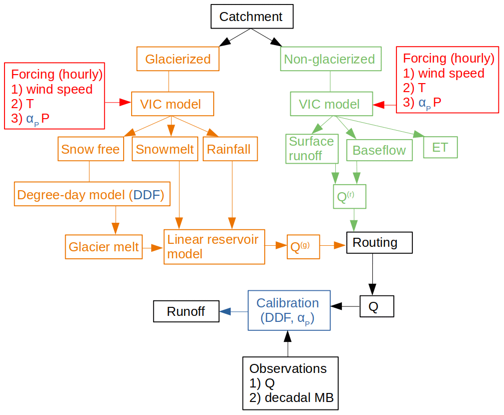
We divided each studied catchment into two parts, the glacierised and non-glacierised ones. On the non-glacierised part, we ran another VIC model (Liang et al., 1996) to compute the surface runoff, baseflow, and evapotranspiration at hourly time steps (Fig. 3). On the glacierised part, a separate VIC model run at hourly time steps was used to get the snowmelt, and a temperature-index model (Hock, 2003) was used to obtain the glacier melt (Fig. 3). The additional glacier module was needed since the VIC model does not have the capability to compute glacier melt (Liang et al., 1996). A similar approach to represent glacier melt was used in existing VIC model studies in the region (Zhang et al., 2013; Zhao et al., 2015; Chandel and Ghosh, 2021). Hourly hydrological fluxes of the non-glacierised and glacierised parts within each grid box were combined and routed (Lohmann et al., 1998) to obtain the total runoff at the catchment outlet. In this step, the flow from each grid box was partitioned into the fast and slow components using hydrographs parameterised with Bf and Ks, , and (Lohmann et al., 1998). The total hourly runoff produced from each grid box was routed downstream in the direction of steepest descent using a linearised Saint-Venant equation (Lohmann et al., 1998).
3.2.1 Hydrological model
The VIC (version 4.2.d, accessible from https://vic.readthedocs.io/en/master/, last access: 23 January 2023; Liang et al., 1996) is a semi-distributed macro-scale hydrological model which simulates the fluxes of water and energy for a grid-based representation of a catchment using physically based parameterisations of hydrological processes (Liang et al., 1996). In this model, water can only enter a grid box from the atmosphere, and once water reaches the river channel, it cannot flow back into the grid box. These assumptions limit the applicability of the model to a larger grid size (e.g. a grid size of 0.25∘ which was used here). The VIC model considers sub-grid heterogeneity in surface topography, land cover, and subsurface soil properties. Different vegetation classes are represented by tiles covering a fraction of the grid box, and an area-weighted sum over the tiles obtains various hydrological fluxes for each grid box. The VIC model partitions the input precipitation at each grid box into rain and snow based on a threshold temperature Tth. It uses a two-layered snowpack, computing the snowmelt at a given elevation with an energy-balance approach. A surface-albedo parameterisation incorporating the effects of snowfall and ageing of snow, snow-sublimation, and refreezing of meltwater within the snowpack are included in the model (Andreadis et al., 2009). Evapotranspiration is computed by the Penman–Monteith equation (Liang et al., 1996) as the sum of canopy evaporation, bare soil evaporation, and transpiration for each vegetation class. The VIC model allows multiple subsurface soil layers, and here, we used three of them. The partitioning between surface runoff and infiltration into the top layer is done using a variable infiltration curve (Liang et al., 1996) controlled by the parameter binf. The bottom layer produces the baseflow depending on the moisture content with a maximum allowed baseflow of Dsmax. At low soil moisture (below a fraction Ws of the maximum allowed soil moisture, and up to a fraction Ds of Dsmax), the baseflow is linear in it. Beyond this linear regime, a non-linear ARNO recession curve determines baseflow (Liang et al., 1996). The chosen values of the above five VIC model parameters are given in Table S2.
Dictated by the resolution of ERA5 input data, the model was run at a spatial resolution and at hourly time steps. The Chandra (upper Dudhkoshi) catchment covered parts of 11 (6) ERA5 grid boxes (Fig. 2a and b), with fractional grid cover in the range 2.5 %–92 % (2 %–68 %). The static input parameters included soil properties (Fischer et al., 2008), land use (Friedl and Sulla-Menashe, 2019), vegetation information (Rodell et al., 2004), and elevation distribution (Farr et al., 2007) for each grid box. We used 10 elevation bands with width in the range 100–300 m depending on the elevation range within the grid box. A minimal set of meteorological forcing parameters, namely bias-corrected air temperature, scaled precipitation, and wind speed from ERA5 reanalysis (Hersbach et al., 2020) over the period 1980–2018, were used to force the model. For model spin-up, we extended the meteorological input data back by repeating the data from 1980 to 1984.
3.2.2 Glacier model
On the glacierised grids of each catchment, a separate VIC model computed the snowmelt and snow-covered fraction of each elevation band (Fig. 3). A minimal temperature-index model (Hock, 2003) was chosen to simulate the ice melt over the corresponding snow-free areas. This one-parameter model is easy to calibrate and is expected to work better for ice cover than for snow cover due to a relatively low seasonal variability of ice albedo (Hock, 2003). The glacier-melt module was forced with the bias-corrected ERA5 air temperature, while taking into account the elevation of the band using a mean monthly lapse rate (Fig. S2). The degree-day factors (DDFs) for each of the catchments were calibrated simultaneously against the observed glacier mass balance and catchment runoff using a Bayesian method (see Sect. 3.2.3). The snowmelt, ice melt, and rainfall on the glaciers that were routed using a linear reservoir model (Hannah and Gurnell, 2001), obtained the glacier runoff. The model used two parallel reservoirs: a slow reservoir with time constant Kslow for routing the snowmelt, and a fast reservoir with time constant Kfast for routing the sum of the ice melt and the rainfall (e.g. Hannah and Gurnell, 2001). Catchment-wise glacier mass balance was computed by subtracting the total ice melt and snowmelt from the total snowfall over the glacierised parts.
The present glacier module did not consider snow redistribution within or between the glacierised and non-glacierised parts of the catchment via avalanching (Laha et al., 2017) or wind redistribution. We did not consider any baseflow contribution from the glacierised parts assuming the negligible permeability of the bedrock. Also, the present model did not consider the effect of the supraglacial debris layer on melting since only 4 %–7 % of the studied catchments consist of debris-covered ice (Scherler et al, 2018). A simple inclusion of the melt-inhibiting effects of the debris layer (e.g. Azam and Srivastava, 2020) may not necessarily lead to an improved estimation of sub-debris melt. For example, the strong melt enhancements at the ice cliffs and/or ponds on the debris-covered surface (e.g. Miles et al., 2022) are often ignored in these models. The available estimates of the extent (e.g. Herreid and Pellicciotti, 2020) and thickness estimates (e.g. Rounce et al., 2018) have large uncertainties as well. Here, we verified that a simplified sub-debris melt scheme (Azam and Srivastava, 2020), which does not consider the variation of debris thickness, induced only small (∼3 %) insignificant changes in the summer runoff compared to the corresponding uncertainties (∼10 %). The effect of snow redistribution driven by wind and gravity in the rugged Himalayan topography are also difficult to capture in any coarse-scale model like the present one. As we are calibrating the observed mass balance of glaciers and catchment runoff, it may take care of the effects of these two factors to some extent.
We assumed a static glacier cover here as the observed percentage loss of glacier area over the simulation period was small (1 %–5 % per decade) for both catchments (Table 1). Biases due to such a static-glacier approximation were found to be small for another glacierised Himalayan catchment over the same period (Azam and Srivastava, 2020). A dynamic description of glaciers within the glacio–hydrological model is needed only for predicting the long-term changes in runoff when potential changes in glacier extent is large (e.g. Kraaijenbrink et al., 2017).
3.2.3 Model calibration
With the limited set of observations available for the studied catchments, calibrating a large number of tunable parameters may not ensure a better representation of the relevant processes (Jost et al., 2012) and may lead to overfitting. It may also suffer from equifinality issues (Beven and Freer, 2001; Jost et al., 2012), where more than one parameter combination reproduces the observed runoff. For example, in glacierised catchments, the same runoff output can be generated by models which use different combinations of the precipitation-scale factor and DDF (Azam and Srivastava, 2020). These models will, however, yield different relative contributions of glaciers to the total runoff, and obtain different climate sensitivities. To avoid the possibility of overfitting, we calibrated only two model parameters: (1) precipitation-scale factor αP and (2) DDF of ice. To ensure a unique best-fit pair of the above parameters, we simultaneously fitted the available summer runoff and glacier mass-balance data (e.g. Van Tiel et al., 2020b) using a Bayesian procedure as discussed below. For the rest of the VIC model parameters, we used the central values of the recommended range (Table S2). Note that these uncalibrated VIC model parameter values were similar to that of the corresponding calibrated values used in some of the studies from the region (e.g. Zhang et al., 2013; Zhao et al., 2015; Bhattacharya et al., 2019; Chandel and Ghosh, 2021). This suggested that the VIC model parameters used here to describe the two Himalayan catchments were representative ones. These model parameter values are listed in Table S2.
To calibrate for the parameters αP and DDF, we used a Bayesian method (e.g. Tarantola, 2005). For given a set of available observations d and a set of model parameters θ, the posterior probability of the model parameters given the observations was
where p(θ) was the prior distribution of the model parameters αP and DDF. We assumed a uniform prior distribution over the range of values reported over High Mountain Asia: 0.7–2.5 for αP (Huss and Hock, 2015; Bhattacharya et al., 2019; Azam and Srivastava, 2020), and 2–16 mm ∘C−1 d−1 for DDF (Singh et al., 2000; Nepal, 2016; Azam et al., 2019). The conditional probability p(d|θ) of the observations d given the model parameter θ was assumed to be a bivariate normal distribution (e.g. Rounce et al., 2020; Werder et al., 2020), i.e. a normally distributed residual for both discharge and glacier mass balance:
where the superscripts “obs” and “mod” denoted the observed and modelled values, respectively. Here, Qi was the weekly summer runoff, and the summation was over all the years with observed runoff data. The jth observed regional geodetic glacier mass balance for each catchment was denoted by bj. This summation was over eight such observations (Bolch et al., 2011; Gardelle et al., 2012; Nuimura et al., 2012; Vincent et al., 2013; Vijay and Braun, 2016; Brun et al., 2017; King et al., 2017; Mukherjee et al., 2018; Maurer et al., 2019; Shean et al., 2020) for each of the catchments as listed in Table S3. The uncertainties and incorporated the errors in the model (σmod) and the observation (σobs). Each of these errors was assumed to be a constant having the following values: was taken to be ∼20 % of the mean summer runoff of the catchments, which is a conservative estimate given the previously reported 5 % error discharge measured using the same method for other Himalayan catchments (e.g. Singh et al., 2005). For both catchments, was taken to be 0.32 m w.e. yr−1, which was the maximum uncertainty associated with the observed regional geodetic glacier mass balance used in this study (Table S3). The values of and were assumed to be 0.15 (0.17) m yr−1 and 0.24 (0.27) m w.e. yr−1, respectively for the Chandra (upper Dudhkoshi) catchment. The model errors were computed using an ensemble of 104 model runs, where either a single (26 models) or a pair (78 models) of model parameters out of the 13 listed in Table S2 were perturbed from the central value by ±25% of their expected range. In these runs, except for the perturbed parameter/s, the rest of the parameters were kept at the central value of the corresponding ranges. For calibration, the two-dimensional parameter space was scanned with step sizes of 0.2 for αP, and 0.5 mm ∘C−1 d−1 for DDF. This yielded an ensemble of models for each catchment, with associated weight p(θ|d) as computed using Eq. (1).
3.2.4 Model validation, parameter sensitivity, and uncertainty
The results from the most probable model were used for estimating summer runoff and its components as well as glacier mass balance. All the relevant quantities were computed for all 319 models in the ensemble, and the corresponding weighted standard deviations were used to obtain the 2σ uncertainties. To assess the model performance, the simulated mean summer runoff, decadal glacier mass balance, and glacier-melt contribution were compared with the corresponding modelled and observed values previously reported in the region. As the observed runoff was available for only 3 to 7 years, all of it was utilised for the above calibration without any validation period. For upper Dudhkoshi catchment, the calibration procedure was repeated using data from a set of 4 consecutive years, while the remaining 3 years' data were utilised for validation. This experiment was repeated four times with different choices of calibration period.
Parameter sensitivity of the best-fit model due to the uncertainties in the uncalibrated parameters were evaluated with the help of additional 22 simulations where 1 of the 11 uncalibrated glacio–hydrological model parameters (Table S2) was perturbed by ±25 % of the range of corresponding recommended values. The sensitivity of summer runoff to these 11 parameters was computed at the corresponding optimal values of DDF and αP. Perturbing the parameters one by one in the 11-dimensional parameter space is similar to computing the multidimensional gradient in this space to understand the model sensitivity. An ensemble of 22 model outputs was generated where 1 of the above 11 uncalibrated parameters (Table S2) of the best-fit model was perturbed by ±25 %. To look for possible interactions between parameters, 78 additional simulations were run, where a chosen pair of parameters were simultaneously perturbed.
3.3 Climate sensitivity of summer runoff
The climate sensitivity of specific summer runoff Q (m yr−1) is defined as the change in runoff due to a unit perturbation in a meteorological forcing parameter (e.g. Zheng et al., 2009). Here, we considered the sensitivity of summer runoff Q due to changes in annual precipitation P (m yr−1) and mean summer temperature T (∘C), as summer runoff was 81 %–86 % of the annual runoff in these catchments (Table 1). We did not consider the annual or winter temperature as it is the summer temperature that controls glacier melt (e.g. Pratap et al., 2019).
3.3.1 Climate sensitivities and summer runoff anomalies
The sensitivities of summer runoff (e.g. Zheng et al., 2009) relate the anomalies of summer runoff δQ (m yr−1), annual precipitation δP (m), and summer air temperature δT (∘C) as follows:
where precipitation sensitivity is denoted by (m yr−1 m−1), and temperature sensitivity is denoted by (m yr−1 ∘C−1). In Eq. (3), a possible bilinear interaction term proportional to δTδP (Lang, 1986) was not considered. We confirmed that this correction term, when included in the regression for the catchment studied, was not significant (p<0.05). In order to estimate the sensitivities sT and sP (Eq. 3), we regressed simulated time series of δQ for the catchments during 1997–2018 with the corresponding time series of δT and δP. The sensitivities estimated from the simulated δQ time series over 1997–2018 were validated using that during 1980–1996 by computing the corresponding Nash–Sutcliffe efficiency (NSE) and root mean squared error (RMSE).
We also considered the runoff from the glacierised part of the catchments , and that from the non-glacierised part of the catchments . Here, the notations Q0 and δQ denote the long-term mean and the anomaly for a given year, respectively. The corresponding sensitivities were defined in a similar way and led to the following relations:
The climate sensitivities of glacierised and non-glacierised parts (Eqs. 4 and 5) and the corresponding uncertainties were estimated in the same way as above using the anomalies δQ(g) and δQ(r), along with δP and δT.
Given the instantaneous glacier fraction x, the quantities defined for the glacierised and non-glacierised parts of the catchments are related to those defined for the whole catchment as follows:
On the glacierised part, we estimated the mass-balance sensitivities to the corresponding temperature and precipitation forcing over the period of 1980–2018. The sensitivities were computed by linearly regressing the modelled anomalies of the mass balance to those of the annual precipitation and summer air temperature. The precipitation sensitivity of glacier mass balance was defined to be the mass-balance change due to a 10 % change in precipitation following the convention used in the literature (e.g. Wang et al., 2019).
3.3.2 Variability of summer runoff
The climate sensitivities defined above allow determination of the interannual variability of summer runoff given those of P and T:
where σQ, σP, and σT are standard deviations of Q, P, and T, respectively. An implicit assumption here is that δP and δT are uncorrelated over the simulation period, which we verified to be true at p<0.05 level for both catchments.
We computed σP and σT during 1980–1996 and 1997–2018 from the forcing data, and used Eq. (9) to predict the corresponding σQ. These predictions were validated using the corresponding σQ obtained directly from the simulated summer runoff time series. We analysed the future changes in σQ in the studied catchments due to shrinking glaciers, and the variation of σQ for a set of hypothetical catchments having different x. Note that an empirical non-monotonic dependence of the coefficient of variation of runoff across catchments on the corresponding fractional glacier cover with a minimum at a moderate glacier cover has been termed as the “glacier-compensation effect” (Chen and Ohmura, 1990).
3.3.3 Long-term changes in mean summer runoff
The climate sensitivities defined above can be used to predict the multidecadal changes in summer runoff (ΔQ) for given changes in annual precipitation (ΔP) and mean summer temperature (ΔT). For a change in glacier fraction Δx from the initial value of x0 (i.e. ), the following linear-response equation can be constructed ignoring the terms that were higher order in Δ:
A similar linear-response approach was used to analyse the glacier-compensation effect (Chen and Ohmura, 1990) without explicitly referring to climate sensitivity. Since ERA5 annual precipitation showed low/little spatial variability within the two catchments (Fig. S4), here we ignored the spatial variation of the generated runoff within the off-glacier or glacierised areas. We also assumed that the contribution of the deglacierised area to the changes in summer runoff is well represented by the difference between the mean runoff of the glacierised and non-glacierised parts. Note that climate-sensitivity-based predictions for future changes in runoff are reliable as long as the predicted changes lie within the range of the recent interannual variability of P, T, and Q. Beyond this range, there may be uncontrolled extrapolation errors.
Equation (10) was used to investigate the multidecadal changes in the summer runoff, assuming glacier-loss scenarios in the Chandra and upper Dudhkoshi catchments to be the same as those projected for the Indus and Ganga basins under the RCP2.6 climate scenario (Huss and Hock, 2018). The corresponding temperature projections were obtained from available estimates for the western and eastern Himalaya, respectively (Fig. S8 of Kraaijenbrink et al., 2017). The related precipitation changes, which were not significant within the uncertainties for both regions (Kraaijenbrink et al., 2017), were ignored here. Consequently, the terms with ΔP in Eq. (10) did not contribute to the estimated changes.

Figure 4Panels (a) and (b) show the posterior probability distribution p(θ|d) of the model parameters (αP, DDF) for the Chandra and upper Dushkoshi catchments, respectively (see Sects. 3.2.3 and 4.1). Panels(c) and (d) show the sensitivities of the simulated summer runoff to perturbations in 11 uncalibrated model parameters for the Chandra and upper Dushkoshi catchments, respectively. Here, ±Δ denotes the perturbation of parameters by ±25 % of the corresponding prescribed range (see Sect. 3.2.4, and Table S2).
Under a sustained warming, glacier runoff is expected to show a peak over a multidecadal scale due to the excess meltwater contribution from the shrinking glacier reserve, which is followed by a decline in the runoff as the ice reserve depletes (Huss and Hock, 2018). Following Huss and Hock (2018), we defined “peak water” as the maximum change in runoff of the area that was glacierised at 2000 CE and used Eq. (10) to predict the timing and the magnitude of the “peak water” in the studied catchments. While the glacier boundaries (RGI Consortium, 2017) belonged to 2002, the small changes in glacier area between 2000 and 2002 were ignored for this calculation due to an observed slow rate of glacier area change (Table 1).
4.1 Calibration and validation
The Bayesian calibration method fitted the observed glacier mass balance and the summer runoff data simultaneously, yielding unique best-fit models for both catchments (Fig. 4a and b) and a unique best-fit model with an optimum pair of DDF and αP. This is in contrast with the case where using only discharge data for calibration leads to a family of best-fit models (e.g. Azam and Srivastava, 2020). The most probable DDF values were 5.0 and 7.5 mm d−1 ∘C−1 for the Chandra and upper Dudhkoshi catchments, respectively. These DDF values were in the same ballpark range as previously used in studies in and around the Chandra (Azam et al., 2019; Pratap et al., 2019) and Dudhkoshi catchments (Pokhrel et al., 2014; Khadka et al., 2014; Nepal, 2016). The best-fit αP was 1.4 for both catchments which was within the range of values 0.7–1.5 used in the existing studies in the Himalaya to correct various reanalysis products (Huss and Hock, 2015; Bhattacharya et al., 2019; Azam and Srivastava, 2020).
The calibrated models reproduced the observed summer runoff of the catchments reasonably well (Fig. 5) with RMSEs of 11 % and 12 % of the mean summer runoff, and NSEs of 0.88 and 0.80 for the Chandra and upper Dudhkoshi catchments, respectively. These RMSE and NSE values were comparable to or smaller than those reported in the existing studies from the region (Nepal, 2016; Mimeau et al., 2018; Bhattacharya et al., 2019; Azam et al., 2019; Azam and Srivastava, 2020). Four additional calibration experiments for upper Dudhkoshi catchment, each one using a different set of 4 consecutive years of runoff data for calibration, obtained the most probable models with DDF (7.2±1.5 mm d−1 ∘C−1), αP (1.43±0.06), NSEs (0.79–0.86), and RMSEs (10 %–14 % of mean summer runoff) similar to those mentioned above.
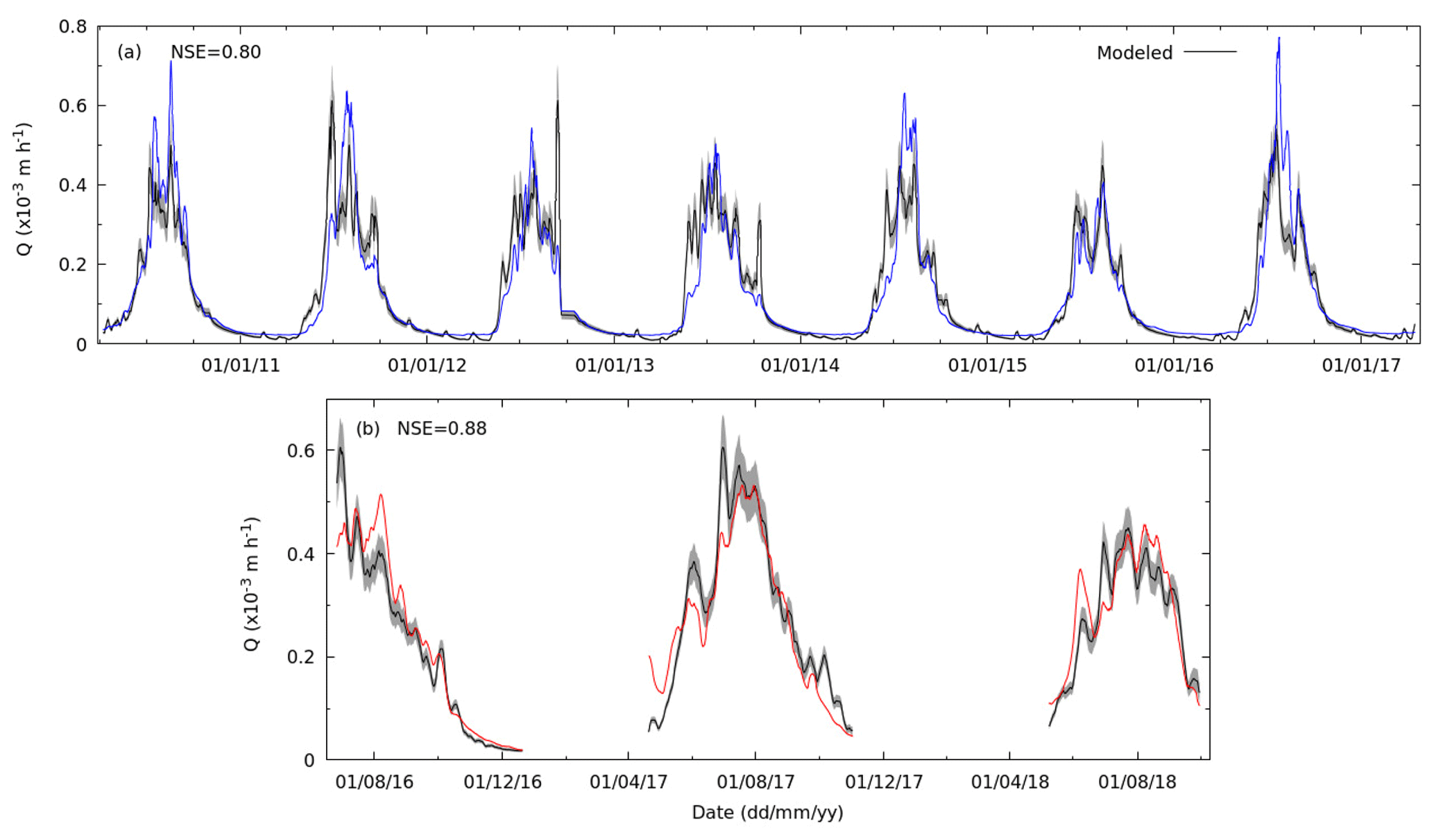
Figure 5Modelled weekly runoff (black lines, with grey bands denoting 2σ uncertainty) compared with the corresponding observations for the (a) upper Dudhkoshi (solid blue line), and (b) Chandra (solid red line) catchments.
To test the statistical significance of the above fits, we computed the probability of having RMSEs of runoff and mass balance equal to or smaller than those in the best-fit model, when the entire model space is sampled uniformly (Fig. S7). For both discharge and glacier mass balance, these probabilities were 0.03 or smaller in both catchments, indicating that the fits were significant at p<0.05 level.
4.2 Simulated runoff and its parameter sensitivity
The simulated mean summer runoff of the Chandra and upper Dudhkoshi catchments over the period 1980–2018 were 1.08±0.08 and 0.81±0.07 m yr−1, respectively (Fig. S6). The corresponding standard deviations were 0.14 and 0.10 m yr−1. The mean summer runoff of the glacierised and the non-glacierised parts of the Chandra catchment were 1.54 and 0.92 m yr−1, respectively. The corresponding values for upper Dudhkoshi catchment were 1.59 and 0.61 m yr−1. In these two catchments, more than 81 % of the simulated annual runoff were during the summer season. In comparison, 7 years of observation from the upper Dudhkoshi catchment (Chevallier et al., 2017) showed a mean specific summer runoff of 0.86±0.05 m yr−1, which was 83 % of the mean annual runoff. Our simulations indicated that glacier runoff contributed 31±12 % and 36±16 % of the total summer runoff in the upper Dudhkoshi and Chandra catchments, with the glacier ice loss amounting to 9 % and 4 % of the respective total summer runoff (Fig. S6).
Existing model studies reported annual runoff of 1.6 m yr−1 during 2000–2010 (Nepal, 2016) and 0.96 m yr−1 during 1981–2015 (Chandel and Ghosh, 2021) for the whole the Dudhkoshi catchment (Fig. 2b), and 0.95 m yr−1 during 2013–2015 (Mimeau et al., 2018) for the Periche subcatchment (Fig. 2b). The last two estimates compared well to those presented above. Existing estimates (Chandel and Ghosh, 2021) of summer runoff (0.87 m yr−1) and glacier runoff (0.76 m yr−1) of the Dudhkoshi catchment were also consistent with our results. No such previous runoff estimates were available for the Chandra catchment. The estimated glacier contributions to runoff obtained here were largely consistent with the existing model studies from the region (Nepal, 2016; Engelhardt et al., 2017; Mimeau et al., 2018; Azam et al., 2019; Chandel and Ghosh, 2021) when the differences in fractional glacier cover were taken into account (Table S4).
The parameter-sensitivity analysis revealed that the absolute changes in summer runoff were less than ∼1.5 % for all the parameters, except Bf and Kslow (Fig. 4b–d). Slightly higher summer-runoff sensitivities (1.8 %–2.5 %) for the two longer timescales Bf and Kslow became less than 1 % when the annual runoff was considered. The additional 78 simulations, where two parameters were perturbed simultaneously, obtained runoff changes almost equal to the sum of those obtained in the corresponding pair of simulations with a single perturbed parameter (Fig. S5). A generally low parameter sensitivity of the summer runoff implied that the present summer runoff estimates were relatively robust to the uncertainties in 11 uncalibrated glacio–hydrological model parameters (Table S2).
4.3 Simulated glacier mass balance and its climate sensitivity
The simulated glacier mass balance for the Chandra and upper Dudhkoshi catchments over 1980–2018 were and m w.e. yr−1. These estimates were comparable to the existing geodetic observations within the uncertainties (Fig. 6c; Table S3). The RMSE between modelled and observed mass balance of the Chandra and upper Dudhkoshi catchments were 0.10 and 0.11 m w.e. yr−1, respectively.
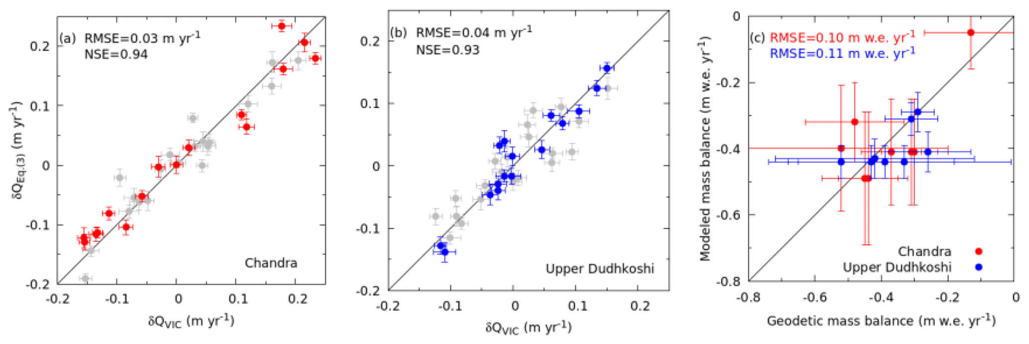
Figure 6The summer runoff anomalies δQEq. (3) as computed using the Eq. (3) are compared with those from the VIC model simulations δQVIC for (a) Chandra and (b) upper Dudhkoshi catchments. The solid red (blue) circles are for the Chandra (upper Dudhkoshi) catchment during the validation period 1980–1996. The solid grey circles denote data from the calibration period 1997–2018. (c) A comparison of the modelled glacier mass balance with the available regional-scale geodetic mass balance for the Chandra (solid red circles) and upper Dudhkoshi (solid blue circles) catchments. The modelled values are over the same period as that of the corresponding observed geodetic mass balance (Table S3). The solid grey line in each plot shows the 1:1 reference line.
The sensitivity of the modelled glacier mass balance to temperature was and m yr−1 ∘C−1 for the Chandra and upper Dudhkoshi catchments, respectively. The corresponding precipitation sensitivities for these catchments were 0.2±0.09 and 0.05±0.05 m yr−1 for a 10 % change in precipitation. These sensitivities were significant at p<0.01 level. The previously reported mass-balance sensitivities at a regional scale (Shea and Immerzeel, 2016; Sakai and Fujita, 2017; Tawde et al., 2017; Wang et al., 2019) and for individual glaciers from the western and central Himalaya (Azam et al., 2014; Wang et al., 2019; Sunako et al., 2019; Azam and Srivastava, 2020) spanned a wide range (Table S8). This possibly reflected the corresponding differences of the climate setting, geometry, and topography of the glaciers studied, along with underlying model assumptions, model calibration, input data sets, and so on. The mass-balance sensitivities obtained in the present study were well within the above range. A relatively higher summer temperature sensitivity of the glaciers of the Chandra catchment compared to those of upper Dudhkoshi was in apparent contradiction with an expected stronger influence of temperature forcing on summer-accumulation-type glaciers due to a conversion between snow and rain (Fujita, 2008; Kumar et al., 2019). However, apart from the precipitation seasonality, mass-balance sensitivity also depends on factors like glacier hypsometry, such that a relatively weaker temperature sensitivity of glaciers in the summer-monsoon-fed Dudhkoshi compared to that in the winter-snow-fed Chandra cannot be ruled out. In fact, a similar trend of mass-balance sensitivities over these two regions were also found in a regional-scale energy-balance model study (Sakai and Fujita, 2017).
4.4 Climate sensitivities of catchment runoff
A linear fit of the summer runoff anomalies to those of summer temperature and annual precipitation (Eq. 3) during 1997–2018 worked well for both the Chandra (R2=0.92) and upper Dudhkoshi (R2=0.93) catchments. These fits obtained respective temperature sensitivities of summer runoff sT of 0.12±0.06 and 0.12±0.09 m yr−1 ∘C−1 for the Chandra and upper Dudhkoshi catchments, respectively. The corresponding best-fit sP were 0.39±0.07 and 0.47±0.13 m yr−1 m−1. These sensitivities were all significant at p<0.01 level. The estimated sensitivities for the two catchments were the same within the limits of uncertainty, and the corresponding percentage changes in runoff were also similar (Table S5). This may be a surprising feature given the contrasting precipitation regimes of the catchments. This issue is discussed later in the text.
The sensitivities computed over the calibration period (1997–2018) reproduced the variability of summer runoff over the validation period (1980–1996) reasonably well (Fig. 6a and b) with RMSE <0.04 m yr−1 and NSE > 0.93. This also validated the use of Eq. (3) to predict the interannual variability of summer runoff in these two catchments. The reported temperature sensitivities of summer runoff over the Himalaya were in the range between 5 %–27 % of summer runoff change per degree Celsius warming, and the precipitation sensitivities of summer runoff were between −0.6 %–16 % of summer runoff due to 10 % changes in P (Fujita and Sakai, 2014; Pokhrel et al., 2014; Azam and Srivastava, 2020) (Table S6). The previously reported temperature and precipitation sensitivities of summer runoff outside the Himalaya were in the range between 9 %–24 % of summer runoff per degree Celsius warming, and 2 %–7 % of summer runoff due to 10 % changes in P (Engelhardt et al., 2015; He, 2021), respectively. The temperature and precipitation sensitivities of summer runoff obtained in the present study, 11 %–14 % of summer runoff per degree Celsius warming and 6 %–9 % of summer runoff due to 10 % changes in P, respectively, were with the above range. It appears that the differences in climate sensitivities of runoff obtained in different studies are mostly due to the corresponding differences in glacier fraction of the catchments studied, as there is a monotonic variation of the sensitivities with glacier fractions (Table S6).
During 1980–2018, the simulated summer runoff in the Chandra and upper Dudhkoshi catchments varied in the range 0.86–1.33 and 0.55–0.98 m yr−1, respectively. The respective ranges of summer temperature were 2.0–5.3 and 1.2–2.3 ∘C, and those of annual precipitation were 1.05–2.10 and 1.17–1.92 m yr−1. As discussed before, the sensitivities estimated above are applicable within the above range of precipitation and temperature forcing. Note that in both catchments, sP was significantly smaller than 1 m yr−1 m−1. This indicated an interannual change of the storage in the glaciers, and a change in evapotranspiration from the off-glacier area in response to the precipitation forcing (see Sect. 4.5 and 4.6).
4.5 Climate sensitivities of glacier runoff
The estimated temperature sensitivities of glacier runoff were 0.41±0.08 and 0.47±0.11 m yr−1 ∘C−1 for the Chandra and upper Dudhkoshi catchments, respectively (significant at p<0.01 level). The corresponding precipitation sensitivities were and 0.00±0.07 m yr−1 m−1 (not significant at p<0.05 level). A compilation of glacier runoff sensitivities (Table S7) indicated that the sensitivities reported here were largely in line with those reported previously in the Himalaya (Fujita and Sakai, 2014; Chandel and Ghosh, 2021) and elsewhere (Anderson et al., 2010; Soruco et al., 2015; Pramanik et al., 2018). Again, both catchments had similar absolute values of and within the corresponding uncertainties. The corresponding percentage sensitivity values were also similar, except for a somewhat higher percentage change in glacier runoff due to unit temperature change in upper Dudhkoshi catchment (Table S5).
Interestingly, summer runoff of both winter-accumulation-type glaciers in the Chandra catchment and summer-accumulation-type glaciers in the upper Dudhkoshi catchment was approximately independent of the corresponding precipitation variabilities. This confirmed the general result, which was derived previously using a simple temperature-index model (Banerjee, 2022), that irrespective of the glacier chosen, the climate setting, or the model used, glacier runoff has a weak to no precipitation sensitivity.
In both studied catchments, a positive precipitation anomaly did not translate into a higher summer runoff of the glaciers (Fig. 7). With increasing precipitation, the rainfall on glacier did not change, and snowmelt showed a very weak (Chandra) to no (upper Dudhkoshi) increase (Fig. 7). This implied that a higher precipitation contributed mostly to a positive storage change (snow accumulation) on the glaciers. In addition, a higher snow cover and/or an association between higher-than-normal precipitation and lower mean temperature (not statistically significant) caused a decline in glacier melt, and amplified the changes in glacier storage change (Fig. 7). These effects combined to yield a nearly precipitation-insensitive glacier runoff in both catchments. In contrast, a higher glacier melt with increasing mean summer temperature caused a relatively high temperature sensitivity of Q(g) in both catchments (Fig. 7). Here, the glaciers effectively acted as infinite reservoirs over an annual scale so that the meltwater volume was limited only by the available energy. A higher temperature implied a higher available energy and thus a higher meltwater flux from the glaciers. These arguments were consistent with a high correlation (r>0.9, p<0.05) between the summer temperature and summer runoff of the glacierised parts for both catchments (Fig. 7).

Figure 7The anomalies of glacier runoff δQ(g) and its components, namely snowmelt δSM(g), glacier ice melt δGM(g), and rainfall δRF(g) for the glacierised parts of the catchments are plotted as a function of the corresponding temperature and precipitation anomalies: (a, b) for the Chandra catchment and (c, d) for the upper Dudhkoshi catchment. The corresponding best-fit straight lines are also shown.
The negligible discussed above implied a stabilisation of the total runoff of the glacierised catchments against precipitation variability (e.g. Van Tiel et al., 2021), as the runoff contribution from the glacierised fraction x was essentially independent of precipitation (Eq. 8). The magnitude of the precipitation sensitivity of catchment runoff sP is thus expected to decrease with the glacier fraction x. This stabilising effect (Banerjee, 2022) is consistent with a reported buffering of catchment runoff by glaciers during the extreme drought years across High Mountain Asia (Pritchard, 2019).
4.6 Climate sensitivity of runoff of the non-glacierised parts
In the non-glacierised parts of the Chandra and upper Dudhkoshi catchments, of 0.02±0.06 and 0.03±0.10 m yr−1 ∘C−1 and of 0.56±0.10 and 0.59±0.12 m yr−1 m−1 were obtained, respectively. These sensitivities were all significant at p<0.01 level. Again, both catchments had similar absolute values of and within the corresponding uncertainties, and the corresponding percentage sensitivity values were similar (Table S5).
Compared to the sensitivities of glacier runoff, the climate sensitivities of the runoff from the non-glacierised parts showed an exactly opposite trend. The summer runoff of the off-glacier areas were relatively insensitive to temperature anomalies but sensitive to precipitation anomalies (Fig. S8). Because of the presence of seasonal snow cover over the non-glacierised parts, a temperature dependence of the summer runoff may be expected. However, the total amount of snowmelt during the summer was limited by the supply of seasonal snow and not by the available energy. This led to a weak response of the total summer runoff from the non-glacierised parts to temperature forcing. This argument was supported by the fact that the summer runoff from the non-glacierised parts was uncorrelated with summer temperature and strongly correlated with summer precipitation (r>0.9, p<0.05). Our results suggest that the precipitation changes in these two catchments caused comparable changes in surface runoff, groundwater/baseflow, and evapotranspiration (Fig. S8). Consequently, about rd of the precipitation anomaly translated to that of the total runoff. Interestingly, evapotranspiration anomalies in the glacier-free parts of Chandra (upper Dudhkoshi) were controlled by the summer temperature (precipitation) (Fig. S8). This suggested a water-limited condition in the summer-monsoon-fed upper Dudhkoshi catchment and an energy-limited condition in the winter-snow-fed Chandra catchment.
4.7 Implications of the estimated climate sensitivities
The above estimated climate sensitivities from glacierised and non-glacierised parts of the catchments suggested and . Thus, Eqs. (3)–(10) can be simplified to the following approximate relations describing the response of the summer runoff to climate variability and change in these two catchments:
These simplified equations suggested that the key parameters that determined the climate response of these glacierised catchments to given climate forcing were and . According to Eq. (11), the precipitation and temperature sensitivity of catchment runoff are essentially given by and , respectively. As both catchments had similar , the corresponding sP was also similar with a slightly smaller value in the Chandra catchment due to a higher fractional glacier cover there. On the other hand, a slightly higher in the upper Dudhkoshi catchment, together with a slightly lower glacier cover there, led to similar sT in the two catchments. Below we discuss the implications of the above simplified linear-response formulae for the future changes in the mean summer runoff and its variability.
4.7.1 Summer runoff variability
Over the calibration period 1997–2018, the Chandra and upper Dudhkoshi catchments had σP of 0.22 and 0.15 m yr−1, and σT of 0.89 and 0.34 ∘C, respectively. These values, together with Eq. (14), predicted σQ of 0.13 and 0.08 m yr−1 for the two catchments which equalled the corresponding values obtained directly from the simulated summer runoff (Fig. 8a). A corresponding close match was also obtained over the validation period of 1980–1996 (Fig. 8a).

Figure 8(a) Predicted σQ using Eq. (14) are compared with the corresponding simulated values for both catchments. The solid and open circles denote data for the periods 1997–2018 and 1980–1996, respectively. Data for the Chandra and upper Dudhkoshi catchments are shown with red and blue symbols, respectively. (b) The solid (dashed) lines show σQ(x) obtained using σP and σT values from 1997–2018 (1980–1996).
Equation (14) can also be used to predict the variation of σQ in these catchments due to the shrinkage glacier cover if σP and σT were to remain unchanged. The shape of the hyperbolic σQ(x) curve for both catchments (Fig. 8b) indicated that major changes in runoff variability may not take place due to the expected glacier loss alone. However, possible changes in σP and σT may drive significant future changes of σQ in these two catchments, as underlined by the difference between the simulated σQ for the two catchments over the periods 1980–1996 and 1997–2018 (Fig. 8b).
4.7.2 Glacier-compensation curve
For a set of hypothetical catchments with different values of x, but similar , , σT and σP, Eq. (14) implies that σQ is a hyperbolic function of x (Fig. 8b). The runoff variability is high in the limit x→0 due to a precipitation sensitive off-glacier runoff with . In the opposite limit of x→1, σQ is again high due to a high temperature sensitivity of glacier runoff, with . These two competing effects yield a minimum in σQ at an intermediate value of x (Fig. 8b) (Banerjee, 2022). This nonmonotonic behaviour of runoff variability with x is well known empirically (e.g. Chen and Ohmura, 1990) and is termed the glacier-compensation effect. The above theoretical explanation of the effect is consistent with a reported strong correlation between runoff and precipitation (temperature) in the limit of small (extensive) glacier cover (Van Tiel et al., 2020a). Note that while Eq. (14) suggests a hyperbolic glacier-compensation curve, some of the existing studies used an empirical parabolic curve (e.g. Chen and Ohmura, 1990). As glacier cover shrink, the summer runoff from both the studied catchments is expected to become more sensitive to precipitation forcing (Eq. 14).
Chen and Ohmura (1990) suggested that the glacier-compensation curve can be utilised to estimate the change in σQ as glacier cover changes. However, recent model simulations indicated that a time-dependent glacier-compensation curve rules out such possibility (Van Tiel et al., 2020a). This is consistent with Eq. (14), which indicates that apart from a changing glacier cover, the compensation curve (and thus σQ) can shift when σP and/or σT changes with time.
4.7.3 Changes in mean summer runoff and prediction of peak water
As discussed before, estimating the future changes mean summer runoff using Eq. (15) requires the changes in summer precipitation or temperature to be within the range of calibration (Sect. 3.2.3). Only for the Chandra catchment, the optimistic RCP2.6 scenario (Fig. S9), temperature change by ∼2050 was within the range of annual temperature over the period 1980–2018, and the present estimates of climate sensitivities could be used safely. The projected mean temperature changes of 1.1 ∘C by 2050 under the RCP2.6 scenario were within the calibration range and obtained a glacier runoff change of 0.27±0.03 m yr−1 (assuming x0=1 at 2000). This was comparable to the corresponding reported estimate of 0.25 m yr−1 for the entire Indus basin (Huss and Hock, 2018).
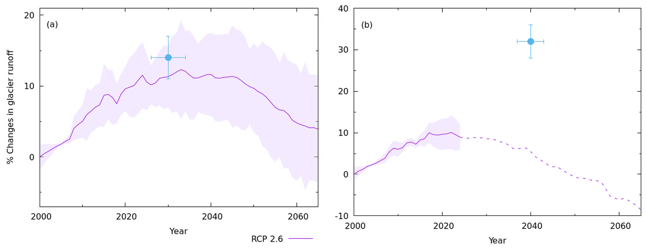
Figure 9The “peak water” due to future glacier changes predicted using Eq. (15) for (a) Chandra, and (b) upper Dudhkoshi catchments, respectively. The solid sky-blue dots represents the corresponding “peak water” as reported in Huss and Hock (2018) for both catchments. The dashed portion of the solid line in the upper Dudhkoshi catchment indicates the corresponding temperature change beyond the calibration range of the catchment. See text for details.
The predicted future changes of glacier runoff in the Chandra catchment, using Eq. (15), reproduced the peak-water effect successfully (Fig. 9). The estimated peak water was 12±8 % of the present glacier runoff, and the estimated timing was 2033±7. In the Chandra catchment, the estimated peak-water in glacier runoff is expected to cause a 0.05 m yr−1 to rise in catchment runoff. This change may not be detectable, given the recent interannual variability of catchment runoff σQ=0.14 m yr−1. Note that the above estimates are comparable to previously predicted peak water of 14±3 % on 2030±4 (Huss and Hock, 2018). It is encouraging that a simple climate-sensitivity-based approach presented here could capture the peak-water effect in the Chandra catchment as well as a state-of-the-art glacio–hydrological model (Huss and Hock, 2018). Note that for the Chandra catchment, our simulated recent glacier runoff, the initial glacier cover, and geodetic mass balance used for calibration were similar to the corresponding values used by Huss and Hock (2018) for the Indus basin.
In the upper Dudhkoshi catchment, we estimated a peak water of 10±4 % of the present glacier runoff, and the estimated timing was 2022±4 (Fig. 9b). This estimated peak water was significantly smaller and quicker compared to that of Huss and Hock (2018). This inconsistency may be related to possible extrapolation errors as the projected temperature changes crossed the range of interannual variability by 2024. Moreover, there were several differences between the two models in this region, which may contribute to the above mismatch. The RGI 4 glacier inventory used by Huss and Hock (2018) had 25 % higher glacier cover in the Ganga basin compared to the RGI 6 used here. In addition, the authors calibrated their model using a geodetic mass-balance record which was twice as negative as the median of the eight geodetic mass-balance records used here. Furthermore, the present estimates of glacier runoff in the upper Dudhkoshi catchment were almost half of that reported by Huss and Hock (2018) for the Ganga basin. The above differences likely led to a corresponding large difference in the modelled climate sensitivities of glacier runoff between the present study and that of Huss and Hock (2018) in this region.
In this paper, we simulate the summer runoff of the Chandra (western Himalaya) and upper Dudhkoshi (eastern Himalaya) catchments over 1980–2018, using the VIC model augmented with a temperature-index glacier-melt module. Calibrating two model parameters using a Bayesian method that simultaneously fits the available summer runoff and decadal-scale geodetic glacier mass balance, our simulation obtained a statistically significant fit to the available observations. The interannual variability of the simulated summer runoff is then utilised to obtain the climate sensitivity of summer runoff to summer temperature and annual precipitation forcing. Despite their contrasting climate regimes, the eastern and the western Himalayan catchments show similar climate sensitivities of the total summer runoff, and that generated from glacierised and non-glacierised parts of the catchments. The simulated climate sensitivities of summer runoff to temperature and precipitation forcing in the catchments reveal interesting patterns: the precipitation sensitivities of the summer runoff of the non-glacierised parts of the catchments are high, but those of the glacierised parts are negligible. In contrast, the temperature sensitivities of summer runoff of glaciers are high, but those of the non-glacierised parts are negligible. The estimated climate sensitivities of summer runoff are also used to obtain analytical insights into several well-known characteristics of the climate response of runoff from glacierised catchments, including the buffering effect, glacier-compensation effect, and the peak-water effect. For the two Himalayan catchments, our approximate analysis suggests that the impacts of the future glacier loss on the long-term mean and variability of catchment runoff may not be detectable, given the relatively large interannual runoff variability in these catchments. However, with a depleting glacier cover, the variability of summer runoff in these two catchments is likely to become more sensitive to precipitation variability. Despite the limitations like the simplifying model assumptions, and the calibration with a limited dataset, the present study brings out the usefulness of a climate-sensitivity-based approach to understand and predict the future changes in runoff of glacierised catchments in the Himalaya.
The VIC model can be downloaded from https://github.com/UW-Hydro/VIC/releases/tag/VIC.4.2.d (Hamman, 2016). The additional codes developed here for glacier-melt modelling and routing can be accessed at https://osf.io/7une2/ (Laha, 2022). All the hydrometeorological observations used here for the upper Dudhkoshi and Chandra catchments are available from https://doi.org/10.23708/000521 (Chevallier et al., 2017) and the Head, Himalayan Cryosphere Studies, NCPOR (email: hcryo@ncpor.res.in), upon request.
The supplement related to this article is available online at: https://doi.org/10.5194/hess-27-627-2023-supplement.
AB conceived the study, and developed the theoretical framework. SL ran the simulations. SL and AB did the data analysis. AB wrote the manuscript with inputs from SL. AS, PS, and MT did the field measurements at the Chandra catchment and analysed the field data. All the authors participated in the discussions and edited the manuscript.
The contact author has declared that none of the authors has any competing interests.
Publisher's note: Copernicus Publications remains neutral with regard to jurisdictional claims in published maps and institutional affiliations.
The study is funded under the HiCOM initiative by ESSO-NCPOR, MoES (grant no. NCAOR/2018/HiCOM/04). Sourav Laha acknowledges INSPIRE Research fellowship (grant no. IF 170526). Argha Banerjee acknowledges support from MoES (grant no. MoES/PAMC/H&C/79/2016-PC-II). We thank the French Agence Nationale de la Recherche (references ANR-09-CEP-0005-04/PAPRIKA and ANR-13-SENV-0005-03/PRESHINE) for sharing the hydrometeorological data in the upper Dushkoshi catchment. We greatly benefited from discussions with Subimal Ghosh, Pradeep P. Mujumdar, and Raghu Murtugudde. Vikram Chandel, Ela Chawla, Arijeet Dutta, and Sneha Potghan helped with the VIC model setup and input data.
This research has been supported by the National Centre for Polar and Ocean Research, Ministry of Earth Sciences (grant no. NCAOR/2018/HiCOM/04).
This paper was edited by Erwin Zehe and reviewed by Lei Wang and one anonymous referee.
Amante, C. and Eakins, B. W.: ETOPO1 1 Arc-Minute Global Relief Model: Procedures, Data Sources and Analysis, NOAA Technical Memorandum NESDIS NGDC-24, National Geophysical Data Center, NOAA, https://doi.org/10.7289/V5C8276M, 2009. a
Anderson, B., Mackintosh, A., Stumm, D., George, L., Kerr, T., Winter-Billington, A., and Fitzsimons, S. Climate sensitivity of a high-precipitation glacier in New Zealand, J. Glaciol., 56, 114-128, https://doi.org/10.3189/002214310791190929, 2010. a
Andreadis, K. M., Storck, P., and Lettenmaier, D. P.: Modeling snow accumulation and ablation processes in forested environments, Water Resour. Res., 45, W05429, https://doi.org/10.1029/2008WR007042, 2009. a
Azam, M. F. and Srivastava, S.: Mass balance and runoff modelling of partially debris-covered Dokriani Glacier in monsoon-dominated Himalaya using ERA5 data since 1979, J. Hydrol., 590, 125432, https://doi.org/10.1016/j.jhydrol.2020.125432, 2020. a, b, c, d, e, f, g, h, i, j, k, l, m
Azam, M. F., Wagnon, P., Vincent, C., Ramanathan, A., Linda, A., and Singh, V. B.: Reconstruction of the annual mass balance of Chhota Shigri glacier, Western Himalaya, India, since 1969, Ann. Glaciol., 55, 69–80, https://doi.org/10.3189/2014AoG66A104, 2014. a
Azam, M. F., Wagnon, P., Vincent, C., Ramanathan, A. L., Kumar, N., Srivastava, S., Pottakkal, J. G., and Chevallier, P.: Snow and ice melt contributions in a highly glacierized catchment of Chhota Shigri Glacier (India) over the last five decades, J. Hydrol., 574, 760–773, https://doi.org/10.1016/j.jhydrol.2019.04.075, 2019. a, b, c, d, e, f, g, h
Azam, M. F., Kargel, J. S., Shea, J. M., Nepal, S., Haritashya, U. K., Srivastava, S., Maussion, F., Qazi, N., Chevallier, P., Dimri, A. P., Kulkarni, A. V., Graham, C. J., and Bahuguna, I.: Glaciohydrology of the Himalaya-Karakoram, Science, 373, eabf3668, https://doi.org/10.1126/science.abf3668, 2021. a, b, c
Banerjee, A.: A weak precipitation sensitivity of glacier runoff, Geophys. Res. Lett., 49, e2021GL096989, https://doi.org/10.1029/2021GL096989, 2022. a, b, c, d, e, f
Banerjee, A., Patil, D., and Jadhav, A.: Possible biases in scaling-based estimates of glacier change: a case study in the Himalaya, The Cryosphere, 14, 3235–3247, https://doi.org/10.5194/tc-14-3235-2020, 2020. a
Beven, K. and Freer, J.: Equifinality, data assimilation, and uncertainty estimation in mechanistic modelling of complex environmental systems using the GLUE methodology, J. Hydrol., 249, 11–29, https://doi.org/10.1016/S0022-1694(01)00421-8, 2001. a
Bhattacharya, T., Khare, D., and Arora, M.: A case study for the assessment of the suitability of gridded reanalysis weather data for hydrological simulation in Beas river basin of North Western Himalaya, Appl. Water Sci., 9, 110, https://doi.org/10.1007/s13201-019-0993-x, 2019. a, b, c, d, e
Bolch, T., Pieczonka, T., and Benn, D. I.: Multi-decadal mass loss of glaciers in the Everest area (Nepal Himalaya) derived from stereo imagery, The Cryosphere, 5, 349–358, https://doi.org/10.5194/tc-5-349-2011, 2011. a
Brun, F., Berthier, E., Wagnon, P., Kaab, A., and Treichler, D.: A spatially resolved estimate of High Mountain Asia glacier mass balances from 2000 to 2016, Nat. Geosci., 10, 668–673, https://doi.org/10.1038/ngeo2999, 2017. a
Chandel, V. S. and Ghosh, S.: Components of Himalayan River Flows in a Changing Climate, Water Resour. Res., 57, e2020WR027589, https://doi.org/10.1029/2020WR027589, 2021. a, b, c, d, e, f, g
Chen, J. and Ohmura, A.: On the influence of Alpine glaciers on runoff, IAHS Publ., 193, 117–125, 1990. a, b, c, d, e, f
Chevallier, P., Delclaux, F., Wagnon, P., Neppel, L., Arnaud, Y., Esteves, M., Koirala, D., Lejeune, Y., Hernandez, F., Muller, R., Chazarin, J.-P., Boyer, J.-F., and Sacareau, I.: Paprika – Preshine hydrology data sets in the Everest Region (Nepal), 2010–18, PAPREDATA [data set], https://doi.org/10.23708/000521, 2017. a, b, c, d
Dooge, J. C. I., Bruen, M., and Parmentier, B.: A simple model for estimating the sensitivity of runoff to long-term changes in precipitation without a change in vegetation, Adv. Water Resour., 23, 153–163, https://doi.org/10.1016/S0309-1708(99)00019-6, 1999. a
Engelhardt, M., Schuler, T. V., and Andreassen, L. M.: Sensitivities of glacier mass balance and runoff to climate perturbations in Norway, Ann. Glaciol., 56, 79–88, https://doi.org/10.3189/2015AoG70A004, 2015. a
Engelhardt, M., Ramanathan, A. L., Eidhammer, T., Kumar, P., Landgren, O., Mandal, A., and Rasmussen, R.: Modelling 60 years of glacier mass balance and runoff for chhota shigri glacier, western himalaya, northern India, J. Glaciol., 63, 618–628, https://doi.org/10.1017/jog.2017.29, 2017. a
Farr, T. G., Rosen, P. A., Caro, E., Crippen, R., Duren, R., Hensley, S., Kobrick, M., Paller, M., Rodriguez, E., Roth, L., Seal, D., Shaffer, S., Shimada, J., Umland, J., Werner, M., Oskin, M., Burbank, D., and Alsdorf, D.: The shuttle radar topography mission, Rev. Geophys., 45, RG2004, https://doi.org/10.1029/2005RG000183, 2007. a
Fischer, G., Nachtergaele, F., Prieler, S., van Velthuizen, H. T., Verelst, L., and Wiberg, D.: Global Agro-ecological Zones Assessment for Agriculture (GAEZ 2008), IIASA, Laxenburg, Austria and FAO, Rome, Italy, https://www.fao.org/soils-portal/data-hub/soil-maps-and-databases/harmonized-world-soil-database-v12/en/ (last access: 23 January 2023), 2008. a
Friedl, M. and Sulla-Menashe, D.: MCD12Q1 MODIS/Terra+Aqua Land Cover Type Yearly L3 Global 500 m SIN Grid V006, NASA EOSDIS Land Processes DAAC [data set], https://doi.org/10.5067/MODIS/MCD12Q1.006, 2019. a
Fujita, K.: Effect of precipitation seasonality on climatic sensitivity of glacier mass balance, Earth Planet. Sc. Lett., 276, 14–19, https://doi.org/10.1016/j.epsl.2008.08.028, 2008. a
Fujita, K. and Sakai, A.: Modelling runoff from a Himalayan debris-covered glacier, Hydrol. Earth Sys. Sci., 18, 2679–2694. https://doi.org/10.5194/hess-18-2679-2014, 2014. a, b, c, d, e
Gardelle, J., Berthier, E., and Arnaud, Y.: Impact of resolution and radar penetration on glacier elevation changes computed from DEM differencing, J. Glaciol., 58, 419-422, https://doi.org/10.3189/2012JoG11J175, 2012. a
Hamman, J.: VIC 4.2.d source code, GitHub [code], https://github.com/UW-Hydro/VIC/releases/tag/VIC.4.2.d (last access: 23 January 2023), 2016. a
Hannah, D. M. and Gurnell, A. M.: A conceptual, linear reservoir runoff model to investigate melt season changes in cirque glacier hydrology, J. Hydrol., 246, 123–141, https://doi.org/10.1016/S0022-1694(01)00364-X, 2001. a, b
He, Z.: Sensitivities of hydrological processes to climate changes in a Central Asian glacierized basin, Front. Water, 3, 46, https://doi.org/10.3389/frwa.2021.683146, 2021. a
Herreid, S. and Pellicciotti, F.: The state of rock debris covering Earth’s glaciers, Nat. Geosci., 13, 621–627, https://doi.org/10.1038/s41561-020-0615-0, 2020. a
Hersbach, H., Bell, B., Berrisford, P., Hirahara, S., Horányi, A., Munoz-Sabater, J., Peubey, C., Radu, R., Schepers, D., Simmons, A., Soci, C., Abdalla, S., Abellan, X., Balsamo, G., Bechtold, P., Biavati, G., Bidlot, J., Bonavita, M., Chiara, G. D., Dahlgren, P., Dee, D., Diamantakis, M., Dragani, R., Flemming, J., Forbes, R., Fuentes, M., Geer, A., Haimberger, L., Hogan, R., Hólm, E., Janisková, M., Keeley, S., Laloyaux, P., Lopez, P., Lupu, C., Radnoti, G., Rosnay, P., Rozum, I., Vamborg, F., Villaume, S., and Thépaut, J.: The ERA5 global reanalysis, Q. J. Roy. Meteorol. Soc., 146, 1999–2049, https://doi.org/10.1002/qj.3803, 2020. a, b, c
Hock, R.: Temperature index melt modelling in mountain areas, J. Hydrol., 282, 104–115, https://doi.org/10.1016/S0022-1694(03)00257-9, 2003. a, b, c
Hock, R., Jansson, P., and Braun, L. N.: Modelling the response of mountain glacier discharge to climate warming, in: Global change and mountain regions, Springer, Dordrecht, 243–252, https://doi.org/10.1007/1-4020-3508-X_25, 2005. a
Huss, M. and Hock, R.: A new model for global glacier change and sea-level rise, Front. Earth Sci., 3, 54, https://doi.org/10.3389/feart.2015.00054, 2015. a, b, c
Huss, M. and Hock, R.: Global-scale hydrological response to future glacier mass loss, Nat. Clim. Change, 8, 135–140, https://doi.org/10.1038/s41558-017-0049-x, 2018. a, b, c, d, e, f, g, h, i, j, k, l
Johnson, E. and Rupper, S.: An examination of physical processes that trigger the albedo-feedback on glacier surfaces and implications for regional glacier mass balance across High Mountain Asia, Front. Earth Sci., 8, 129, https://doi.org/10.3389/feart.2020.00129, 2020. a
Jost, G., Moore, R. D., Menounos, B., and Wheate, R.: Quantifying the contribution of glacier runoff to streamflow in the upper Columbia River Basin, Canada, Hydrol. Earth Syst. Sci., 16, 849–860, https://doi.org/10.5194/hess-16-849-2012, 2012. a, b
Khadka, D., Babel, M. S., Shrestha, S., Tripathi, N. K.: Climate change impact on glacier and snow melt and runoff in Tamakoshi basin in the Hindu Kush Himalayan (HKH) region, J. Hydrol., 511, 49–60, https://doi.org/10.1016/j.jhydrol.2014.01.005, 2014. a
King, O., Quincey, D. J., Carrivick, J. L., and Rowan, A. V.: Spatial variability in mass loss of glaciers in the Everest region, central Himalayas, between 2000 and 2015, The Cryosphere, 11, 407–426, https://doi.org/10.5194/tc-11-407-2017, 2017. a
Koppes, M., Rupper, S., Asay, M., and Winter-Billington, A.: Sensitivity of glacier runoff projections to baseline climate data in the Indus River basin, Front. Earth Sci., 3, 59, https://doi.org/10.3389/feart.2015.00059, 2015. a
Kraaijenbrink, P. D. A., Bierkens, M. F. P., Lutz, A. F., and Immerzeel, W. W.: Impact of a global temperature rise of 1.5 degrees Celsius on Asias glaciers, Nature, 549, 257–260, https://doi.org/10.1038/nature23878, 2017. a, b, c, d, e
Kumar, P., Saharwardi, M. S., Banerjee, A., Azam, M. F., Dubey, A. K., and Murtugudde, R.: Snowfall variability dictates glacier mass balance variability in Himalaya-Karakoram, Scient. Rep., 9, 1–9, https://doi.org/10.1038/s41598-019-54553-9, 2019. a, b
Laha, S.: Codes for the preprint: Climate sensitivity of the summer runoff of two glacierised Himalayan catchments with contrasting climate, OSF [code], https://osf.io/7une2 (last access: 23 January 2023), 2022. a
Laha, S., Kumari, R., Singh, S., Mishra, A., Sharma, T., Banerjee, A., Nainwal, H. C., and Shankar, R.: Evaluating the contribution of avalanching to the mass balance of Himalayan glaciers, Ann. Glaciol., 58, 110–118, https://doi.org/10.1017/aog.2017.27, 2017. a
Lang, H.: Forecasting meltwater runoff from snow-covered areas and from glacier basins, In River flow modelling and forecasting, Springer, Dordrecht, 99–127, https://doi.org/10.1007/978-94-009-4536-4_5, 1986. a
Liang, X., Wood, E. F., and Lettenmaier, D. P.: Surface soil moisture parameterization of the VIC-2L model: Evaluation and modification, Global Planet. Change, 13, 195–206, https://doi.org/10.1016/0921-8181(95)00046-1, 1996. a, b, c, d, e, f, g, h
Lohmann, D., Raschke, E., Nijssen, B., and Lettenmaier, D. P.: Regional scale hydrology: I. Formulation of the VIC-2L model coupled to a routing model, Hydrolog. Sci. J., 43, 131–141, https://doi.org/10.1080/02626669809492107, 1998. a, b, c
Maurer, J. M., Schaefer, J. M., Rupper, S., and Corley, A.: Acceleration of ice loss across the Himalayas over the past 40 years, Sci. Adv., 5, eaav7266, https://doi.org/10.1126/sciadv.aav7266, 2019. a
Miles, E. S., Steiner, J. F., Buri, P., Immerzeel, W. W., and Pellicciotti, F.: Controls on the relative melt rates of debris-covered glacier surfaces. Environ. Res. Lett., 17, 064004, https://doi.org/10.1088/1748-9326/ac6966, 2022. a
Mimeau, L., Esteves, M., Zin, I., Jacobi, H.-W., Brun, F., Wagnon, P., Koirala, D., and Arnaud, Y.: Quantification of different flow components in a high-altitude glacierized catchment (Dudh Koshi, Himalaya): some cryospheric-related issues, Hydrol. Earth Syst. Sci., 23, 3969–3996, https://doi.org/10.5194/hess-23-3969-2019, 2019. a, b, c
Mukherjee, K., Bhattacharya, A., Pieczonka, T., Ghosh, S., and Bolch, T.: Glacier mass budget and climate reanalysis data indicate a climatic shift around 2000 in Lahaul-Spiti, western Himalaya, Climatic Change, 148, 219–233, https://doi.org/10.1007/s10584-018-2185-3, 2018. a
Nepal, S.: Impacts of climate change on the hydrological regime of the Koshi river basin in the Himalayan region, J. Hydro-Environ. Res., 10, 76–89, https://doi.org/10.1016/j.jher.2015.12.001, 2016. a, b, c, d, e, f
Nie, Y., Pritchard, H. D., Liu, Q., Hennig, T., Wang, W., Wang, X., Liu, S., Nepal, S., Samyn, D., Hewitt, K., and Chen, X.: Glacial change and hydrological implications in the Himalaya and Karakoram, Nat. Rev. Earth Environ., 2, 91–106, https://doi.org/10.1038/s43017-020-00124-w, 2021. a
Nuimura, T., Fujita, K., Yamaguchi, S., and Sharma, R. R.: Elevation changes of glaciers revealed by multitemporal digital elevation models calibrated by GPS survey in the Khumbu region, Nepal Himalaya, 1992–2008, J. Glaciol., 58, 648–656, https://doi.org/10.3189/2012JoG11J061, 2012. a
Oulkar, S. N., Thamban, M., Sharma, P., Pratap, B., Singh, A. T., Patel, L. K., Pramanik, A., and Ravichandran, M.: Energy fluxes, mass balance, and climate sensitivity of the Sutri Dhaka Glacier in the western Himalaya, Front. Earth Sci., 10, 949735, https://doi.org/10.3389/feart.2022.949735, 2022. a
Pokhrel, B. K., Chevallier, P., Andreassian, V., Tahir, A. A., Arnaud, Y., Neppel, L., Bajracharya, O. R., and Budhathoki, K. P.: Comparison of two snowmelt modelling approaches in the Dudh Koshi basin (eastern Himalayas, Nepal), Hydrolog. Sci. J., 59, 1507–1518, https://doi.org/10.1080/02626667.2013.842282, 2014. a, b, c, d
Pramanik, A., Van Pelt, W., Kohler, J., and Schuler, T. V.: Simulating climatic mass balance, seasonal snow development and associated freshwater runoff in the Kongsfjord basin, Svalbard (1980–2016), J. Glaciol., 64, 943–956, https://doi.org/10.1017/jog.2018.80, 2018. a
Pratap, B., Sharma, P., Patel, L., Singh, A. T., Gaddam, V. K., Oulkar, S., and Thamban, M.: Reconciling High Glacier Surface Melting in Summer with Air Temperature in the Semi-Arid Zone of Western Himalaya, Water, 11, 1561, https://doi.org/10.3390/w11081561, 2019. a, b, c
Pritchard, H. D.: Asia's shrinking glaciers protect large populations from drought stress, Nature, 569, 649–654, https://doi.org/10.1038/s41586-019-1240-1, 2019. a
RGI Consortium: Randolph Glacier Inventory – A Dataset of Global Glacier Outlines, Version 6, NSIDC – National Snow and Ice Data Center, Boulder, Colorado, USA, https://doi.org/10.7265/4m1f-gd79, 2017. a, b
Rodell, M., Houser, P. R., Jambor, U., Gottschalck, J., Mitchell, K., Meng, C.-J., Arsenault, K., Cosgrove, B., Radakovich, J., Bosilovich, M., Entin, J. K., Walker, J. P., Lohmann, D., and Toll, D.: The Global Land Data Assimilation System, B. Am. Meteorol. Soc., 85, 381–394, https://doi.org/10.1175/BAMS-85-3-381, 2004. a
Rounce, D. R., King, O., McCarthy, M., Shean, D. E., and Salerno, F.: Quantifying debris thickness of debris-covered glaciers in the Everest region of Nepal through inversion of a subdebris melt model, J. Geophys. Res.-Earth, 123, 1094–1115, https://doi.org/10.1029/2017JF004395, 2018. a
Rounce, D. R., Khurana, T., Short, M. B., Hock, R., Shean, D. E., and Brinkerhoff, D. J.: Quantifying parameter uncertainty in a large-scale glacier evolution model using Bayesian inference: application to High Mountain Asia, J. Glaciol., 66, 175–187, https://doi.org/10.1017/jog.2019.91, 2020. a
Sakai, A. and Fujita, K.: Contrasting glacier responses to recent climate change in high-mountain Asia, Scient. Rep., 7, 1–8, https://doi.org/10.1038/s41598-017-14256-5, 2017. a, b, c
Sanjay, J., Krishnan, R., Shrestha, A. B., Rajbhandari, R., and Ren, G. Y.: Downscaled climate change projections for the Hindu Kush Himalayan region using CORDEX South Asia regional climate models, Adv. Clim. Change Res., 8, 185–198, https://doi.org/10.1016/j.accre.2017.08.003, 2017. a
Scherler, D., Wulf, H., and Gorelick, N.: Global assessment of supraglacial debris‐cover extents, Geophys. Res. Lett., 45, 11798–11805, https://doi.org/10.1029/2018GL080158, 2018. a
Shea, J. M. and Immerzeel, W. W.: An assessment of basin-scale glaciological and hydrological sensitivities in the Hindu Kush–Himalaya, Ann. Glaciol., 57, 308–318, https://doi.org/10.3189/2016AoG71A073, 2016. a
Shean, D. E., Bhushan, S., Montesano, P., Rounce, D. R., Arendt, A., and Osmanoglu, B.: A systematic, regional assessment of high mountain Asia glacier mass balance, Front. Earth Sci., 7, 363, https://doi.org/10.3389/feart.2019.00363, 2020. a
Sherpa, S. F., Wagnon, P., Brun, F., Berthier, E., Vincent, C., Lejeune, Y., Arnaud, Y., Kayastha, R. B., and Sinisalo, A.: Contrasted surface mass balances of debris-free glaciers observed between the southern and the inner parts of the Everest region (2007–15), J. Glaciol., 63, 637–651, https://doi.org/10.1017/jog.2017.30, 2017. a
Singh, A. T., Sharma, P., Sharma, C., Laluraj, C. M., Patel, L., Pratap, B., Oulkar, S., and Thamban, M.: Water discharge and suspended sediment dynamics in the Chandra River, Western Himalaya, J. Earth Syst. Sci., 129, 1–15, https://doi.org/10.1007/s12040-020-01455-4, 2020. a
Singh, P. and Kumar, N.: Effect of orography on precipitation in the western Himalayan region, J. Hydrol., 199, 183–206, https://doi.org/10.1016/S0022-1694(96)03222-2, 1997. a
Singh, P., Kumar, N., and Arora, M.: Degree–day factors for snow and ice for Dokriani Glacier, Garhwal Himalayas, J. Hydrol., 235, 1–11, https://doi.org/10.1016/S0022-1694(00)00249-3, 2000. a
Singh, P., Haritashya, U. K., Ramasastri, K. S., and Kumar, N.: Diurnal variations in discharge and suspended sediment concentration, including runoff‐delaying characteristics, of the Gangotri Glacier in the Garhwal Himalayas, Hydrol. Process., 19, 1445–1457, https://doi.org/10.1002/hyp.5583, 2005. a
Soncini, A., Bocchiola, D., Confortola, G., Minora, U., Vuillermoz, E., Salerno, F., Viviano, G., Shrestha, D., Senese, A., Smiraglia, C., and Diolaiuti, G.: Future hydrological regimes and glacier cover in the Everest region: The case study of the upper Dudh Koshi basin, Sci. Total Environ., 565, 1084–1101, https://doi.org/10.1016/j.scitotenv.2016.05.138, 2016. a
Soruco, A., Vincent, C., Rabatel, A., Francou, B., Thibert, E., Sicart, J. E., and Condom, T.: Contribution of glacier runoff to water resources of La Paz city, Bolivia (16∘ S), Ann. Glaciol., 56, 147–154, https://doi.org/10.3189/2015AoG70A001, 2015. a
Sunako, S., Fujita, K., Sakai, A., and Kayastha, R. B.: Mass balance of Trambau Glacier, Rolwaling region, Nepal Himalaya: in-situ observations, long-term reconstruction and mass-balance sensitivity, J. Glaciol., 65, 605–616, https://doi.org/10.1017/jog.2019.37, 2019. a
Tarantola, A. Inverse problem theory and methods for model parameter estimation, Society for Industrial and Applied Mathematics, https://doi.org/10.1137/1.9780898717921, 2005. a
Tawde, S., Kulkarni, A., and Bala, G.: An estimate of glacier mass balance for the Chandra basin, western Himalaya, for the period 1984–2012, Ann. Glaciol., 58, 99–109, https://doi.org/10.1017/aog.2017.18, 2017. a
Vano, J. A., Das, T., and Lettenmaier, D. P.: Hydrologic sensitivities of Colorado River runoff to changes in precipitation and temperature, J. Hydrometeorol., 13, 932–949, https://doi.org/10.1175/JHM-D-11-069.1, 2012. a, b, c
Van Tiel, M., Kohn, I., Van Loon, A. F., and Stahl, K.: The compensating effect of glaciers: Characterizing the relation between interannual streamflow variability and glacier cover, Hydrol. Process., 34, 553–568, https://doi.org/10.1002/hyp.13603, 2020a. a, b
Van Tiel, M., Stahl, K., Freudiger, D., and Seibert, J.: Glacio‐hydrological model calibration and evaluation. Wiley Interdisciplin. Rev.: Water, 7, e1483, https://doi.org/10.1002/wat2.1483, 2020b. a
Van Tiel, M., Van Loon, A. F., Seibert, J., and Stahl, K.: Hydrological response to warm and dry weather: do glaciers compensate?, Hydrol. Earth Syst. Sci., 25, 3245–3265, https://doi.org/10.5194/hess-25-3245-2021, 2021. a
Vijay, S. and Braun, M.: Elevation change rates of glaciers in the Lahaul-Spiti (Western Himalaya, India) during 2000–2012 and 2012–2013, Remote Sens., 8, 1038, https://doi.org/10.3390/rs8121038, 2016. a
Vincent, C., Ramanathan, Al., Wagnon, P., Dobhal, D. P., Linda, A., Berthier, E., Sharma, P., Arnaud, Y., Azam, M. F., Jose, P. G., and Gardelle, J.: Balanced conditions or slight mass gain of glaciers in the Lahaul and Spiti region (northern India, Himalaya) during the nineties preceded recent mass loss, The Cryosphere, 7, 569–582, https://doi.org/10.5194/tc-7-569-2013, 2013. a
Wang, R., Liu, S., Shangguan, D., Radic, V., and Zhang, Y.: Spatial heterogeneity in glacier mass-balance sensitivity across High Mountain Asia, Water, 11, 776, https://doi.org/10.3390/w11040776, 2019. a, b, c
Werder, M. A., Huss, M., Paul, F., Dehecq, A., and Farinotti, D.: A Bayesian ice thickness estimation model for large-scale applications, J. Glaciol., 66, 137–152, https://doi.org/10.1017/jog.2019.93, 2020. a
Zhang, L., Su, F., Yang, D., Hao, Z., and Tong, K.: Discharge regime and simulation for the upstream of major rivers over Tibetan Plateau, J. Geophys. Res.-Atmos., 118, 8500–8518, https://doi.org/10.1002/jgrd.50665, 2013. a, b
Zhao, Q., Zhang, S., Ding, Y. J., Wang, J., Han, H., Xu, J., Zhao, C., Guo, W., and Shangguan, D.: Modeling hydrologic response to climate change and shrinking glaciers in the highly glacierized Kunma Like River Catchment, Central Tian Shan, J. Hydrometeorol., 16, 2383–2402, https://doi.org/10.1175/JHM-D-14-0231.1, 2015. a, b
Zheng, H., Zhang, L., Zhu, R., Liu, C., Sato, Y., and Fukushima, Y.: Responses of streamflow to climate and land surface change in the headwaters of the Yellow River Basin, Water Resour. Res., 45, W00A19, https://doi.org/10.1029/2007WR006665, 2009. a, b, c, d, e