The suitability of a seasonal ensemble hybrid framework including data-driven approaches for hydrological forecasting

Hydrological forecasts are important for operational water management and near-future planning, even more so in light of the increased occurrences of extreme events such as floods and droughts. Having a forecasting framework, which is flexible in terms of input forcings and forecasting locations (local, regional, or national) that can deliver this information in fast and computational efficient manner, is critical. In this study, the suitability of a hybrid forecasting framework, combining data-driven approaches and seasonal (re)forecasting information from dynamical models, to predict hydrological variables was explored. Target variables include discharge and surface water levels for various stations at a national scale, with the Netherlands as the focus. Five different machine learning (ML) models, ranging from simple to more complex and trained on historical observations of discharge, precipitation, evaporation, and seawater levels, were run with seasonal (re)forecast data, including the European Flood Awareness System (EFAS) and ECMWF seasonal forecast system (SEAS5), of these driver variables in a hindcast setting. The results were evaluated using the evaluation metrics, i.e. anomaly correlation coefficient (ACC), continuous ranked probability (skill) score (CRPS and CRPSS), and Brier skill score (BSS), in comparison to a climatological reference hindcast. Aggregating the results of all stations and ML models revealed that the hindcasting framework outperformed the climatological reference forecasts by roughly 60 % for discharge predictions (80 % for surface water level predictions). Skilful prediction for the first lead month, independently of the initialization month, can be made for discharge. The skill extends up to 2–3 months for spring months due to snowmelt dynamic captured in the training phase of the model. Surface water level hindcasts showed similar skill and skilful lead times. While the different ML models showed differences in performance during a testing and training phase using historical observations, running the ML framework in a hindcast setting showed only minor differences between the models, which is attributed to the uncertainty in seasonal forecasts. However, despite being trained on historical observations, the hybrid framework used in this study shows similar skilful predictions to previous large-scale forecasting systems. With our study, we show that a hybrid framework is able to bring location-specific skilful seasonal forecast information with global seasonal forecast inputs. At the same time, our hybrid approach is flexible and fast, and as such, a hybrid framework could be adapted to make it even more interesting to water managers and their needs, for instance, as part of a fast model-predictive control framework.

1 Introduction

Forecasting in combination with local system knowledge plays an important role in increasing the readiness for imminent extreme events such as floods and droughts. Especially over the last few years, where the effects and impacts of climate change have become more and more distinct, with an increasing recurrence of extreme events requiring adaptive planning based on skilful forecasts. For instance, knowledge of upcoming water surplus or shortage is not only important to limit damage to infrastructure and impacts on society during floods, and also to increase and sustain the water availability prior, but also during droughts.

Over the past few years, platforms of openly available forecasting services and data sets that deliver meteorological and hydrological predictions have increased. These data sets can differ in lead time (e.g. short to medium range, sub-seasonal, and seasonal timescales) and include uncertainty by consisting of various numbers of ensemble members. Examples of openly available seasonal forecasting system are the operational European Flood Awareness System (EFAS; Thielen et al., 2009; Arnal et al., 2018) and the Global Flood Awareness System (GloFAS; Alfieri et al., 2013), and the ECMWF's latest seasonal forecasting system of SEAS5 (Johnson et al., 2019). Forecasting systems like these are run by large-scale, physically based models (e.g. LISFLOOD; Van Der Knijff et al., 2010; De Roo et al., 2000, in the case of EFAS), which require a lot of information regarding parametrization, can be slow and computationally intensive, and require large data storage facilities. Another example of forecasting systems facing similar challenges are multimodel ensemble systems, which combine several general circulation models and hydrological models (Wanders et al., 2019; Samaniego et al., 2019).

Even though there is continuous improvement in terms of ease of use and interoperability, the main challenges of handling such large, computationally and data-intensive systems remain. Furthermore, Samaniego et al. (2019) highlighted that, in cases where forecasting systems are used for decision-making, prediction horizons, spatial scales, model choices, storage, and computational requirements, and reported variables can limit the applicability of forecasting systems for local water management. We hypothesize that incorporating data-driven approaches to support seasonal forecasting systems can be beneficial not only in terms of reducing computational requirements but also increasing their flexibility and data use. Especially if the forecasting system can be kept simple, for example, regarding input forcings or the complexity of the forecasting set-up, the threshold of applying it on various spatial and temporal scales would be lowered even further. This would, for example, bridge the gap from large-scale to local forecasting systems and make it more readily applicable for creating efficient operational settings and supporting local water management. In this study, we explore these opportunities by incorporating data-driven approaches in a seasonal forecasting framework, combining both local and global information.

Data-driven approaches, including machine learning (ML) models, have been explored and tested out increasingly in hydrological assessments over the last few years (Shen, 2018; Shen et al., 2021), either as standalone models or also in hybrid settings (coupled with physically based models; Kratzert et al., 2018; Koch et al., 2019). ML can be used for any spatial- and temporal-scale study, as long as there are sufficient data available for training and validation. Besides using local observations and remote sensing information, an upcoming trend is also to incorporate knowledge-based learning (Koch et al., 2021), where ML models are also trained with information provided by physically based models or in hybrid model set-ups. ML has not only shown to be promising in simulating hydrological variables such as discharge and groundwater levels but also in contributing to operational water management.

However, most of the previous research focused on successfully simulating past observations or current hydrological states but incorporating ML in a seasonal forecasting framework has only scarcely been explored in the hydrological field. Work by Hunt et al. (2022), which is one of the most recent examples, documents a situation in which long short-term memory (LSTM) models were explored in a hybrid forecasting set-up to predict discharge on a short-term scale.

A substantial issue with respect to using ML for seasonal forecasting is often the limited number of samples for training. This is often resolved by including long climate model simulations for training as an example; however, depending on the scale and resolution, these might not always be ideal for more local studies. Nevertheless, if sufficient local data are available, then it is worthwhile investigating how one can exploit the assets of ML for seasonal forecasting (with a limited complexity regarding the forecasting set-up, computational demand, and handling of large data amounts) to increase the support for water management. This can not only be especially useful for floods but also drought occurrences, where local information has to be available and updated within a short time frame (floods), and changes in water management planning have to be reassessed both ahead of time and at the time of an event to optimize water availability (droughts).

To be able to have such a forecasting system that can support water managers as an example, a first step is to build a framework that can be explored in a so-called hindcasting experiment, where the forecasting framework is tested based on historical observations in near-real time. Once this is successful, the forecasting framework could be switched to seasonal forecasting. The aim of this study is to explore the first step, which is to test the suitability of a hybrid forecasting framework in a hindcast experiment. The framework will build on an existing ML model framework based on a previous study by Hauswirth et al. (2021) in combination with (re)forecast information as input variables. In this study, we want to test the suitability of these models based on their historical performance to forecast discharge and surface water levels in a hindcast setting.

The ML models (trained on historical observations) will be run with seasonal (re)forecasting data replacing the previous input data set consisting of discharge, precipitation, evaporation, and seawater level observations. Running the models with seasonal (re)forecasting information creates an ensemble of the target variables for each station of interest. The focus of the target variables is laid on discharge and surface water levels, with the latter including rivers, streams, and lakes. These ensembles will be analysed and compared with historical observations not only to assess the skill of the ML framework for seasonal forecasting of general hydrological conditions but also extreme events such as droughts by computing different common skill scores to evaluate seasonal forecasting frameworks. Furthermore, the benefits and also the challenges of such a simple set-up will be explored and listed to assess whether the framework is suitable for current practices and whether it opens up possibilities for future assessments.

In the following sections, the study's approach will be laid out, followed by an evaluation of the performance of the hindcast experiment by assessing skill scores both for general situations and droughts. Thereafter, the findings will be summarized, discussed, and put into a bigger context of the field, followed by the main conclusions.

2 Material and methods

This section is divided into subsections covering the general concept of the hybrid hindcast framework used in this study, the seasonal (re)forecast data and its preparation, the data-driven model set-up, and the skill scores used to evaluate the forecasting skills of the hybrid framework.

2.1 Hybrid hindcast framework

The hybrid hindcast framework used in this study can be described as a simple three-block system including the pre-processing of the input data, a main model block including a selection of ML models, and post-processing of the target variable and skill score calculation (Fig. 1). The main model block, which is based on the ML model study of Hauswirth et al. (2021), was run on seasonal (re)forecasting information, which has first undergone the pre-processing block. The hindcast results were evaluated based on different skill scores included in the post-processing block to assess how skilful the hybrid framework is in hindcasting historical observations. The spatial and temporal settings of the hindcast experiment focus on the Netherlands and the time period 1993–2018. Target variables include discharge and surface water level in freshwater bodies for selected stations (69 for discharge and 97 for surface water level) throughout the observation network of the Dutch National Water Authority.

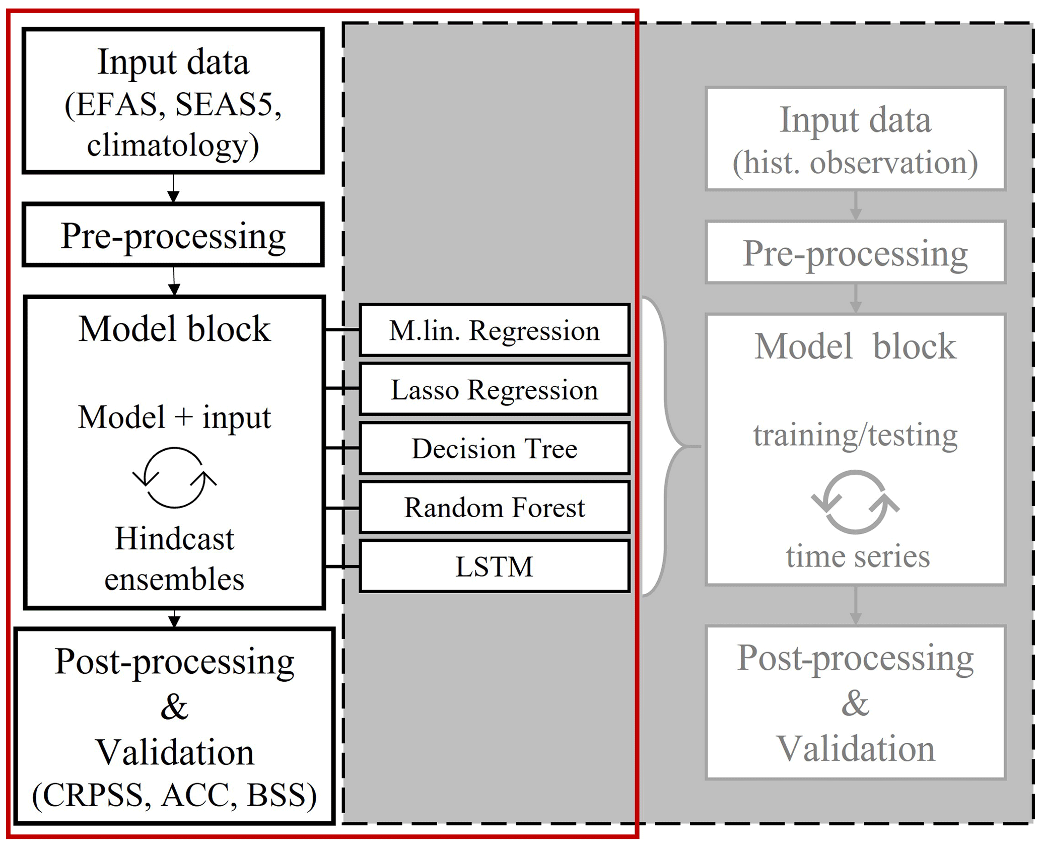
Figure 1 Schematization of a hybrid hindcast framework highlighted in a red frame, with the grey box indicating a model framework previously developed by Hauswirth et al. (2021) and used as a base for the model block.

2.1.1 Data and pre-processing

The input data set, based on seasonal (re)forecasting information, covers the period 1993–2018, including a lead time of 7 months (215 d) and consists of 25 ensemble members (50 from 2017 on). The input data set replaces the previously used historic data of the ML framework, which consists of a simple set of variables including discharge, precipitation, evaporation, and sea level observations at specific locations of the case study area for the time period 1980–2018 (Fig. A1). These variables were chosen as they are part of the observational network of the Dutch National Water Authority and are readily available. Furthermore, the main model block, as defined in Hauswirth et al. (2021), was designed with the idea of being flexible in the sense that input data sets could be easily exchanged by data sets representing the same variables (e.g. seasonal (re)forecasting data). The seasonal (re)forecasting data were obtained from the forecasting systems SEAS5 and EFAS, accessed via the openly available data platform Copernicus Climate Data Store (https://cds.climate.copernicus.eu/#!/home, last access: March 2021). SEAS5 is ECMWF's fifth-generation seasonal forecasting system, providing predictions on atmosphere, ocean, and land surface conditions (Johnson et al., 2019). Meteorological information, including precipitation, u and v wind components, 2 m temperature, surface net solar radiation, and mean sea level pressure were gathered from SEAS5 and were taken from the grid cell that included the original observation location. The latter three variables were used to calculate the Makkink reference potential evaporation (de Bruin and Lablans, 1998). Seasonal (re)forecasting information on discharge was obtained from the European Flood Awareness System (EFAS; Thielen et al., 2009; Wanders et al., 2014; Arnal et al., 2018), a pan-European seasonal hydrological forecasting system which is based on the LISFLOOD model (5×5 km resolution), with SEAS5 used as the meteorological forcing. The same approach of selecting the grid cells including the stations' location of the original input data was taken. Having SEAS5 has a forcing for both the EFAS reforecasts of discharge and, as source for the meteorological input data for the ML framework, enables a consistency in terms of model forcings.

For the sea level data, the water level for the historic period was simulated by using the Pytides Python module. The difference between the observed and Pytides-predicted sea level fluctuations (including only tidal components) was computed to obtain the anomalies. A simple multilinear regression model was then used to compute the final sea level ensemble set based on the u and v wind speed and the previously computed sea level anomalies.

The input data set was processed in a similar manner to that done by Hauswirth et al. (2021), for example, by including the lagged time series of every input variable. This was done in the previous study by using the partial autocorrelation function (PACF) to identify and incorporate significant information content that could explain the historic patterns and additionally be fed to the machine learning in its training phase (Hauswirth et al., 2021). In this case, the seasonal (re)forecasting data in a first step were bias corrected using cumulative density function (CDF) matching approach before extending the input variable by incorporating the lagged times series approach (Wanders et al., 2014).

We additionally prepared an input data set, including water management influence, using the same approach as in Hauswirth et al. (2021). This simulation includes the operational rules of the main infrastructures which are related to the Rhine discharge at Lobith (one of our main input variables) for two specific input locations and two additional observation records of locations based at smaller infrastructures (Fig. A1). We were therefore able to use the same approach regarding the operational rules for the main infrastructures, as these are based on the Rhine discharge that we obtain from the EFAS data set. For the two other additional time series, climatology was used, as operational plans were not available.

For every ML model (representing a station of interest), the input data set after data pre-processing finally consists of a set of ensembles, including the ensemble members of all input variables. The models were run with every set of the ensemble members (e.g. input data set based on first ensemble members of discharge, precipitation, evaporation, and sea level information).

2.1.2 Data-driven model set-up

We applied here a recently developed ML model framework by Hauswirth et al. (2021). This framework has a focus on a simple set-up, using only readily available input data to simulate target variables such as discharge, surface water level (including rivers, streams, and lakes), surface water temperature, and groundwater levels for several stations at a national scale in the Netherlands. The station information and observational records were taken from the national monitoring network and covered 69 discharge, 97 surface water level, 105 surface water temperature, and ∼4000 groundwater stations (Fig. A1, for discharge and surface water level stations). For every station of interest, a ML model was trained on the historic observations of the target variable and the input data set, which consists of the five variables, i.e. precipitation and evaporation from the De Bilt, Rhine discharge at Lobith, Meuse discharge at Eijsden, and sea level observations close to the Haringvliet sluice (Fig. A1). Furthermore, the framework is able to incorporate the influence of water management aspects. This was done by expanding the input data set with a discharge time series of the most important infrastructure, based their operational rules, which is linked to one of the main input variables. Different ML methods were trained and tested based on a $\mathrm{60}\mathit{\%}/\mathrm{40}\mathit{\%}$ train–test split, including time series segments which were chosen randomly. The ML methods incorporated in the study range from simple to more complex methods including multilinear regression (MReg), lasso regression (Lasso), decision tree (DT), and random forest (RF), as well as long short-term memory (LSTM) models. For more information regarding the specific models, model set-up steps, and evaluation, as well as data pre-processing, we refer to Hauswirth et al. (2021).

For this study, the pre-trained models were rerun based on a prepared seasonal (re)forecast input data set. We decided to test out all the original ML models to see whether similar observations regarding their performance and differences could be made. The input data set is made up of the same variables as in the previous study but taken from seasonal (re)forecasting data sets such as EFAS and SEAS5. The models were not retrained, so the input data were used for an extensive validation of the simulation of seasonal forecasting skill. Using the pre-trained models has the benefit of saving computational time, which would have otherwise been needed for testing and training the models. Second, this study aims to test the suitability of this ML framework for seasonal forecasting in an operational setting. In such an operational setting, one would like to keep a consistent modelling framework that has been validated on an extensive hindcast archive. On the other hand, not retraining the models on ensemble data sets limits the potential improvement the model could experience by seeing forecasting data in the training phase. As we want to test the suitability of the developed ML framework for hindcasting, we are putting a focus on the pre-trained model in combination with the seasonal (re)forecast input data set. This allows us to test the performance of the models based on information that the models have definitely not seen before. Running the model based on a seasonal (re)forecast input data set, consisting of several ensemble members, creates an ensemble of time series for the target variables discharge and surface water levels. The same number of ensemble members (25 members, with 50 members from 2017 on) and same lead time (215 d) as the seasonal (re)forecast input data were generated for the target variables. These ensemble simulations of the target variables were then analysed by computing frequently used skill scores.

2.2 Evaluation – skill scores

To evaluate the performance of the hybrid hindcast framework, the target variables were compared to observations at daily, weekly, and monthly temporal scales using different skill scores. These skill scores are shedding a light on various aspect of hindcast skills, for example, overall performance, accuracy, and reliability. Skill scores that are common in the forecasting community and are used here include the continuous ranked probability (skill) score (CRPS and CRPSS), Brier (skill) score (BS and BSS), and anomaly correlation coefficient (ACC). In this study, the hindcasts (including 7 months of lead time) will be addressed by their lead time, where lead one equals the first months of the forecast in which it was initiated, lead two equals the second month after initialization, etc. For the results, the focus will be on weekly and monthly average timescales, which would also be of interest to water managers for mid- to long-term planning.

2.2.1 CRPS and CRPSS

The CRPS, which is one of the most commonly used evaluation benchmarks used in ensemble forecasting studies (Pappenberger et al., 2015), was used to assess the overall performance of the hindcasting framework. It compares the differences in the hindcast and observed cumulative distribution functions (CDFs) and ranges from 0 to infinity. The lower the computed score, the better the performance of the hindcasting framework (Arnal et al., 2018; Pappenberger et al., 2015). Equation (1), taken from Hersbach (2000) (where P(x) is the cumulative density function of the hindcast and P_a (observation probability) is computed), was used, and the CRPS was computed over all ensemble members for each lead day of every hindcast before aggregating it to other temporal scales.

As a skilful benchmark (baseline), we also compare the hindcast framework with a forecasts based on the historical distribution of observations. In other words, for each forecast day, we look at the historical observations for that day and select values for all the years of this historical observation to generate an observation-based climatological hindcast ensemble. Both the hindcast CRPS and the baseline CRPS were used to compute the CRPSS (Eq. 2). The CRPSS range lies between 0 and 1, with 1 indicating the forecast giving the best performance compared to climatology and 0 having no skill compared to climatology.

$$\begin{array}{}\text{(1)}& {\displaystyle }& {\displaystyle }\mathrm{CRPS}=\mathrm{CRPS}\left(P,x_a\right)=\underset{-\mathrm{\infty }}{\overset{\mathrm{\infty }}{\int }}{\left[P\left(x\right)-P_a\left(x\right)\right]}^{\mathrm{2}}\mathrm{d}x\text{(2)}& {\displaystyle }& {\displaystyle }\mathrm{CRPSS}=\mathrm{1}-{\displaystyle \frac{{\mathrm{CRPS}}_{\mathrm{hindcast}}}{{\mathrm{CRPS}}_{\mathrm{baseline}}}}.\end{array}$$

2.2.2 BS and BSS

To determine the accuracy and the performance of the hindcasts for simulating high- and low-flow periods, the BS (Brier, 1950) and BSS can be used. To assess these specific categories, thresholds can be defined, e.g. the lowest 20th percentile data are used to account for droughts similar to other studies (Van Loon and Laaha, 2015). This allows one to analyse events which are either higher or lower than the usual observations for a given month (Candogan Yossef et al., 2017; Wanders and Wood, 2016). This threshold was used for both hindcasts and observations before aggregating the data to the temporal scale of interest and computing the BS. The BS is calculated by Eq. (3), where N equals the number of hindcasting instances, and f and o are the hindcast and observed probability of exceeding a threshold, respectively (Candogan Yossef et al., 2017). Score values range between 0 and 1, whereas 0 indicates the best performance.

$$\begin{array}{}\text{(3)}& {\displaystyle }& {\displaystyle }\mathrm{BS}={\displaystyle \frac{\mathrm{1}}{N}}\sum _{t=\mathrm{1}}^N{\left(f_{\mathrm{t}}-o_{\mathrm{t}}\right)}^{\mathrm{2}}\text{(4)}& {\displaystyle }& {\displaystyle }\mathrm{BSS}=\mathrm{1}-{\displaystyle \frac{{\mathrm{BS}}_{\mathrm{hindcast}}}{{\mathrm{BS}}_{\mathrm{ref}}}}.\end{array}$$

Furthermore, the BSS (Eq. 4) can be used to compare the accuracy and performance of the hindcasting framework compared to a reference system, which is climatology in this case. The same range and interpretation can be used as for CRPSS.

2.2.3 ACC

To measure the quality of the hindcasting framework, the anomaly correlation coefficient (ACC) is computed by using Eq. (5), where (f_t) represents the hindcasts and (o_t) the observations, while $\stackrel{\mathrm{‾}}{f}$ and $\stackrel{\mathrm{‾}}{o}$ are the long-term averages.

$$\begin{array}{}\text{(5)}& \mathrm{ACC}={\displaystyle \frac{\sum _{t=\mathrm{1}}^N\left(f_{\mathrm{t}}-\stackrel{\mathrm{‾}}{f}\right)\left(o_{\mathrm{t}}-\stackrel{\mathrm{‾}}{o}\right)}{\sqrt{\sum _{t=\mathrm{1}}^N{\left(f_{\mathrm{t}}-\stackrel{\mathrm{‾}}{f}\right)}^{\mathrm{2}}\sum _{t=\mathrm{1}}^N{\left(o_{\mathrm{t}}-\stackrel{\mathrm{‾}}{o}\right)}^{\mathrm{2}}}}}.\end{array}$$

The hindcasts and observations were first aggregated to the temporal scale of interest before computing the ACC. The ACC helps to verify the hindcast and observed anomalies compared to the normal correlation, where seasonality can influence the calculation results. Therefore, the ACC can also be seen as a skill score in comparison with the climate. The ACC score ranges from −1 to 1, with 1 representing a perfect correlation between observations and forecast. For representation purposes, the significance level was computed based on the number of observational years (in general), and only stations with fewer than 10 missing observation months were considered (same criteria for station selection were used for the other scores).

3 Results

The results will be presented such that first an overview of the general performance of the hindcast framework for one target variable, the discharge hindcasts, will be given. Subsequently, the focus will be directed towards one model (random forest, RF) and an example station to provide more in-depth insight into the different evaluation scores and differences in temporal resolution. The scores were calculated for all the initialization months of the hindcast and for different temporal resolutions (daily, weekly, and monthly). For demonstration, we highlight the performance of the hindcast framework for selected months, providing weekly to monthly scores, which are temporal scales of interest for long-term water management decisions. Further background information on the evaluation score results based on different initialization months, temporal scales, target variables, and ML models can be found in the Appendix.

3.1 General performance

To obtain an understanding of the overall performance of the hybrid framework for discharge hindcasts, the CRPSS, aggregated over all hindcasts for all stations and all ML models, was computed. This was done by computing all the individual daily CRPSS results of all the hindcasts of every station and methods. The CRPSS results were additionally aggregated by lead day for the different temporal scales before averaging. The average CRPSS (weekly temporal scale) was used for Fig. 2, where the CDFs for the first 12 lead weeks are highlighted, with CRPSS ranging from −1 to 1, with values above 0 indicating the hindcast framework outperforming the climatological reference. As expected, the CRPSS decreases with increasing lead time (with CDF lines moving up, and the zero line being crossed earlier) and naturally converges after 7 weeks. However, up to lead week 12, roughly 60 % of all stations and models show a better performance than the climatological reference. Even better results can be seen for surface water levels (Fig. B1), where up to 80 % show a better performance. Even though the separate evaluation scores can vary slightly between target variable and station (locations shown later on), the overall hindcasting framework shows a positive tendency compared to hindcasts solely based on climatology.

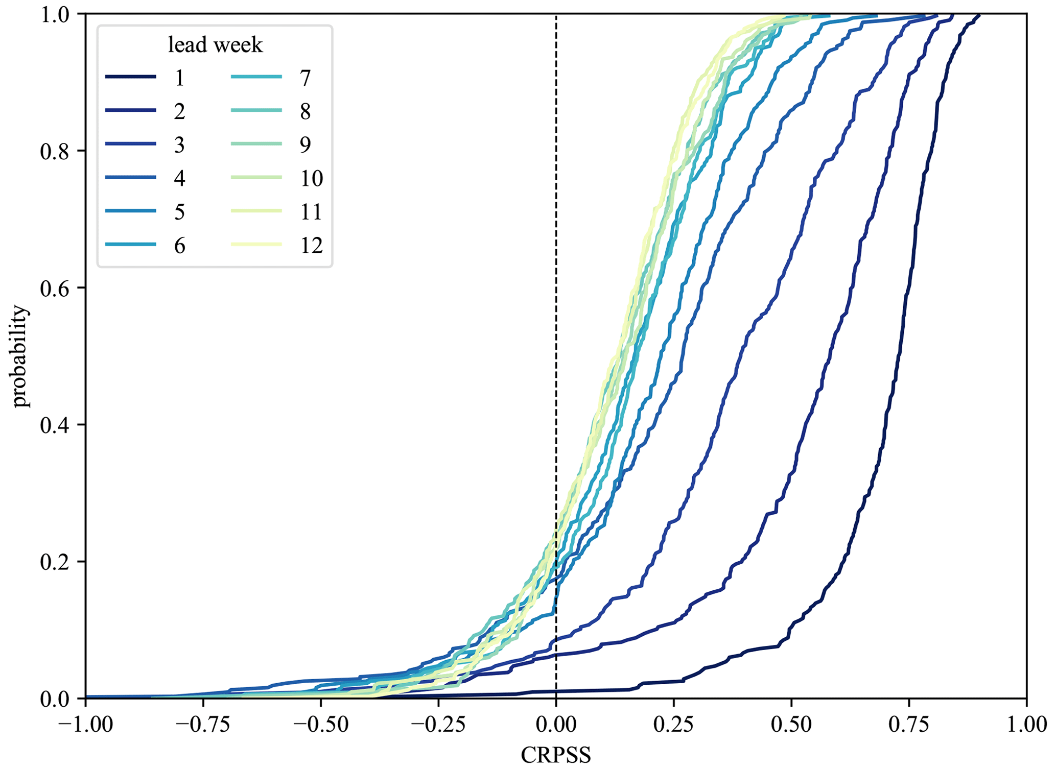
Figure 2 CDFs of weekly CRPSS shown for different lead weeks, with CRPSS being aggregated over all models and stations for discharge hindcasts. CRPSS is decreasing with increasing lead weeks, but even up to 12 weeks, roughly 60 % of all stations and models show a better performance than the reference hindcasts.

We also observe that the hindcast framework shows higher performance compared to the bias-corrected EFAS seasonal (re)forecasting data (Fig. 3), indicating the added benefit of having a hybrid framework that includes locally trained models. In Fig. 3, the CRPSS results for two stations (Lobith and Eijsden), based on the bias-corrected EFAS (for the grid cell where the station is located) and the hybrid framework, are highlighted. Differences not only in skill for larger lead times but also throughout different initialization months can be seen for both stations. Furthermore, despite the EFAS data being bias corrected for the specific locations, the skill, for example, at station Eijsden, is relatively low for some months, indicating that forecasts based on climatology show similar skill. The improvement in local skill is a result of the local training and the ability of the ML model to also use other information (e.g. precipitation and temperature) to further improve its forecast compared to the EFAS system.

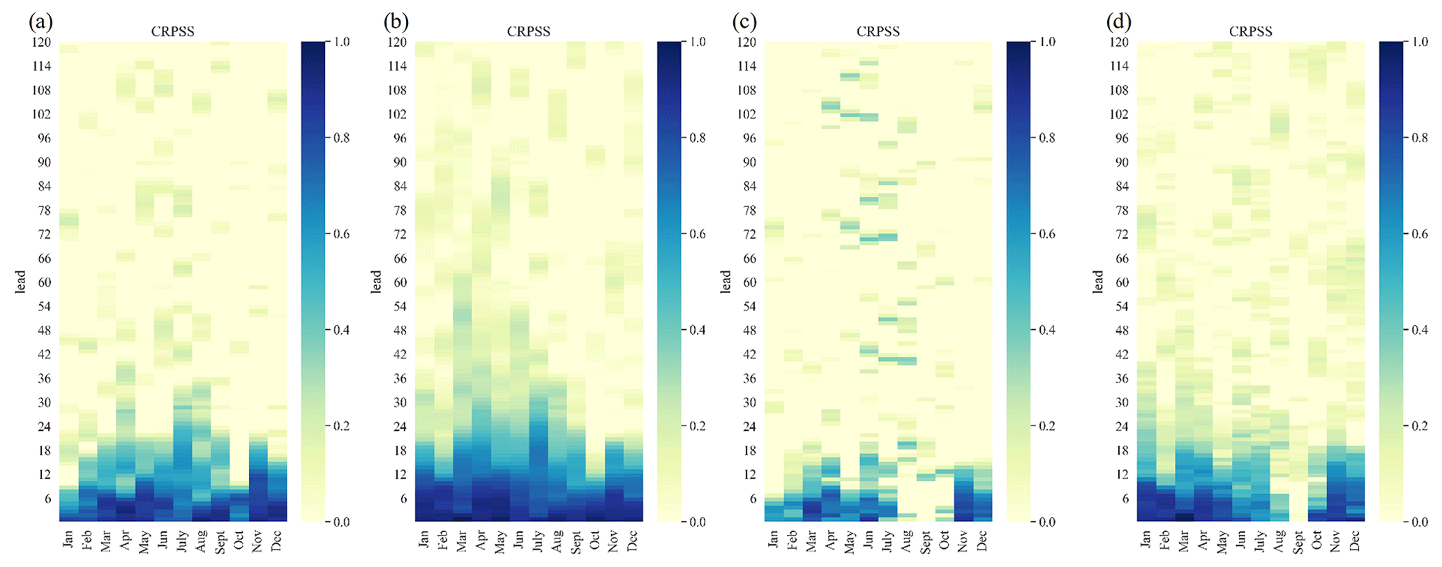
Figure 3 CRPSS (daily) shown for EFAS input data (bias corrected) and hindcasts computed by the hybrid framework for stations Lobith and Eijsden. (a) EFAS at Lobith, (b) hybrid framework at Lobith, (c) EFAS at Eijsden, and (d) hybrid framework at Eijsden. Differences in skill for lead times and also throughout different initialization months can be observed with the hybrid framework, indicating a higher skill for local predictions than the large-scale forecasting system.

During the analysis of the evaluation scores for all the different ML model hindcasts, only minor differences between the models are noticeable, which is seen throughout most stations along the main river network, especially for discharge hindcasts (Fig. 4). Minor differences between methods are observed for surface water level, depending on the station location (Fig. B2), where, for the example stations shown, the more simpler methods show a slightly better skill. The minor differences are likely due to the limited impact of the model selection compared to the inherent uncertainty (represented by the ensemble spread) in the dynamical meteorological and hydrological forecast data. The forecasting skill is likely more dependent on the skill by which the input variables are forecasted, which apparently make the differences in skill between the ML models insignificant in comparison. In addition, the high temporal aggregation (monthly) and post-processing of the results before calculating the different evaluation scores that smooth out the original differences in hindcasts results reduce the differences in performance between models.

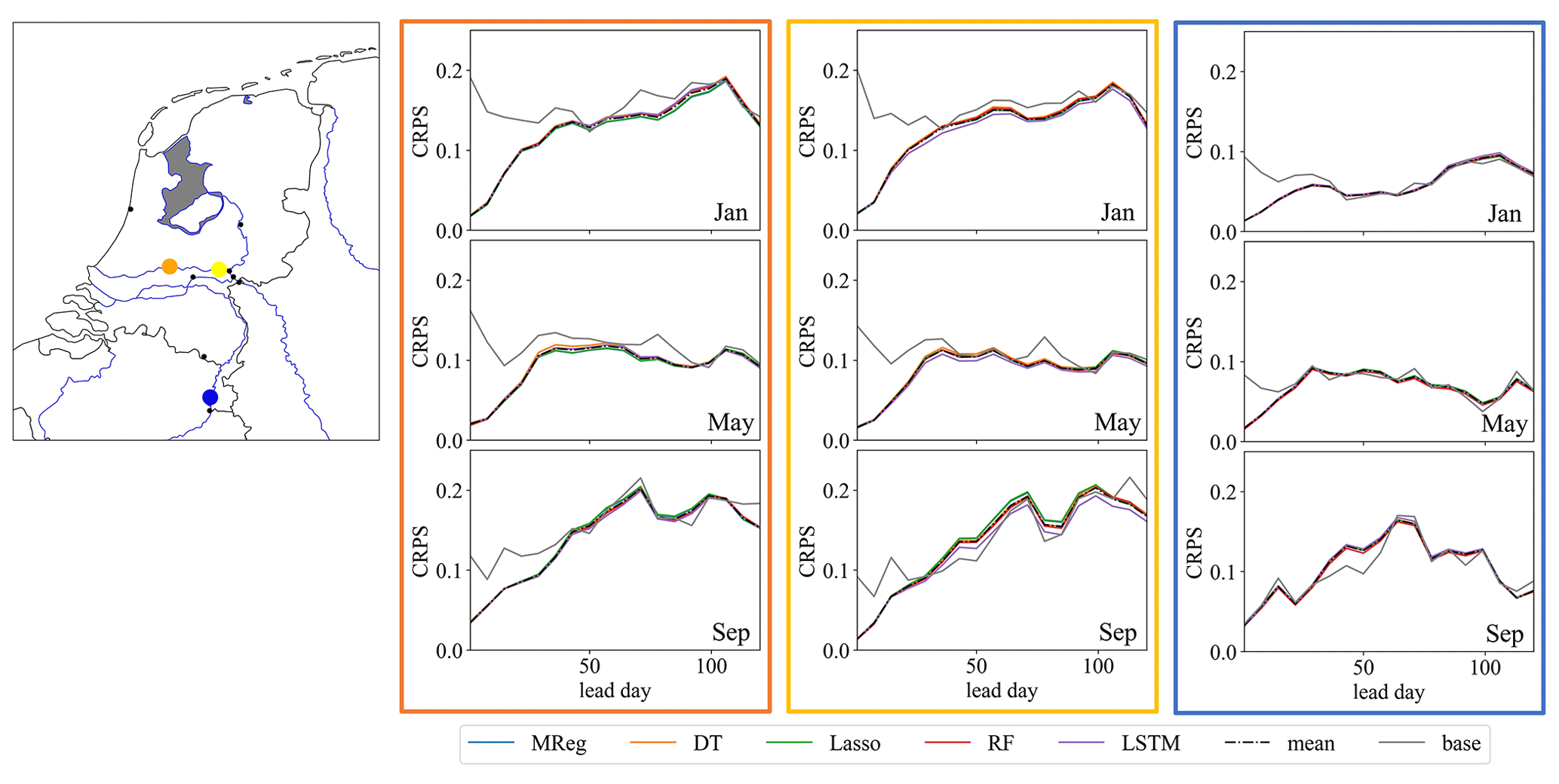
Figure 4 Overview of weekly CRPS values for January, May, and September. Different ML model scores, the average of the ML model score (dashed line), and the climatological reference (grey) are shown for three discharge stations (Hagenstein Boven in orange, Driel in yellow, and Borgharen Dorp in blue). For most months shown and for the first few lead weeks, the CRPS of the hindcast framework shows a lower score than the climatological reference. However, only minor differences between the ML models were observed. Maps were created using the Python package Cartopy (Elson et al., 2022), which uses basemap data made with Natural Earth and © OpenStreetMap contributors 2022. Distributed under the Open Data Commons Open Database License (ODbL) v1.0.

Shifting the focus from the whole hindcast framework to a more detailed exploration of the evaluation metrics, the following paragraphs focus on results of one ML model and later on one example station. As hindcast results indicate that the differences between the models are minor, we will focus on the RF model, which previously already showed a promising performance (Hauswirth et al., 2021). Figure 5 shows the weekly anomaly correlation coefficient (ACC) for the discharge hindcasts at various stations (each represented by a pie chart) throughout the Netherlands for initialization months of (a) January, (b) April, (c) July, and (d) October. The ACC values per week are indicated by the pie slices, arranged clockwise, and their colours, with dark blue indicating a high correlation coefficient while light yellow slices show weeks with a lower coefficient (note that only the significant values are shown). Looking at the results for the different months in Fig. 5 indicates that, for all months shown, the ACC decreases with increasing lead weeks. However, for all months, the first few weeks (minimum of 3–4 weeks) show a high and significant score. This can be observed for all stations along the main river networks, both the Rhine and Meuse, while stations which are located at smaller streams or channels, which are strongly influenced by water management, can be more challenging (e.g. station close to the sea which is located near a shipping channel).

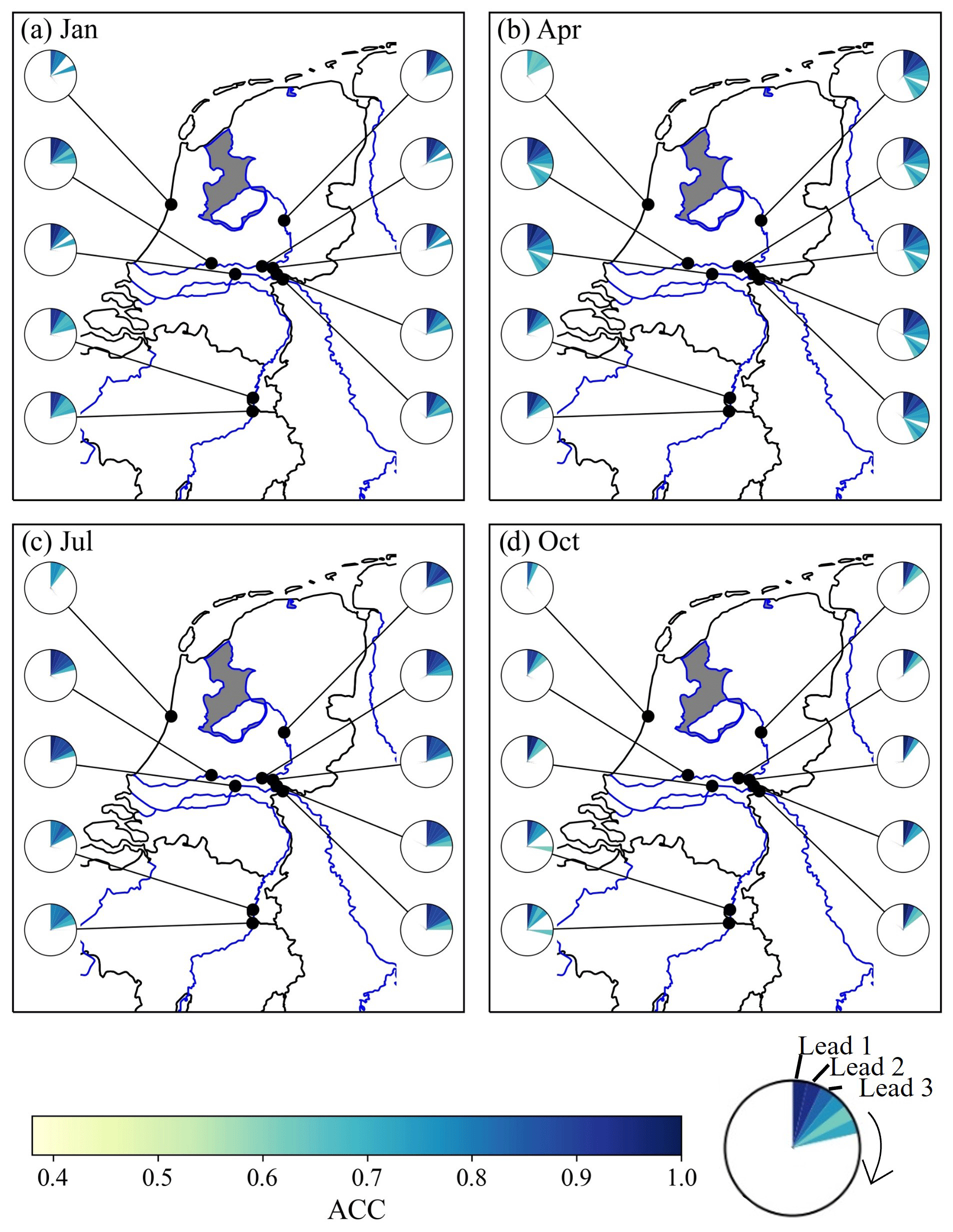
Figure 5 Anomaly correlation coefficient (ACC; weekly) for (a) January, (b) April, (c) July, and (d) October, for discharge hindcasts computed by the RF model, showing the results for different stations (limited selection for visual purposes) in the national monitoring network. Only significant values are shown (indicated by a range of 0.4 and higher). Furthermore, only major river networks are shown, and smaller streams or infrastructures are not highlighted (the station along the coast is placed at a sluice along a stream). Maps were created using the Python package Cartopy (Elson et al., 2022), which uses basemap data made with Natural Earth and © OpenStreetMap contributors 2022. Distributed under the Open Data Commons Open Database License (ODbL) v1.0.

The observations from countrywide ACC analysis are supported by a more detailed analysis for the Hagenstein Boven station located on the Rhine river network, roughly in centre of the Netherlands, and influenced by water management. We clearly see that there are differences in ACC per lead and initialization month, related to the initialization month of the hindcast and the length of the forecast (Fig. 6), that are also already observable in Fig. 5 for the different stations and initialization months. In addition, Fig. 6 shows that the differences on the ACC in temporal aggregation from daily and weekly to monthly temporal scales has a minor impact and that the skill assessment is robust. Significant ACC values can be observed throughout the first lead month for all initialization months. For the early spring and summer months (March–July), significant ACC values for discharge predictions can be seen until 2 months in advance in all temporal aggregation levels. The increase in the significant lead time for the early spring months (March and April) is due to the snowmelt dynamics in the upstream catchment that were captured in the model training period (done prior to this study) and the physical model inputs from the EFAS system at the Lobith and Eijsden stations. The observation of more significant ACC values during the spring months due to the snowmelt dynamic can be found throughout the stations along the Rhine, and this is less pronounced for the stations along the Meuse. Discharge predictions from late summer onwards show lower ACC values, likely due to the lower predictability in atmospheric weather patterns and reduced water storage in highly predictable stores like snow and groundwater. Unrealistically long lead times with significant values are likely due to lower the observation records that can occur throughout the years, despite the selection of stations with limited missing records. Overall, ACC values for the discharge hindcasts show that hindcast anomalies are captured well for lead times up to 1 or 2 months for all initialization months compared to the observed anomalies for a complex station like Hagenstein Boven, which is affected by water management and upstream water reallocation. Furthermore, the hindcast framework was able to capture the general snowmelt dynamic in early spring, resulting in significant values up to a lead time of 2 months at the onset of summer.

Figure 6 ACC results for the discharge hindcasts using the RF model of station Hagenstein Boven over different temporal scales – (a) daily, (b) weekly, and (c) monthly – and different initialization months. Only significant values are shown (indicated by a range of 0.4 and higher).

To check the robustness of the results, we also analysed the forecast performance with the CRPSS and BSS. The CRPSS was computed to assess the general performance in terms of the spread and accuracy of the hindcast framework. Figure 7 represents the weekly CRPSS values for the same example station of Hagenstein Boven in the centre panel. The heatmap gives an overview of the skill score throughout the year, with values ranging from 0 to 1 and values above 0 representing lead weeks in which the hindcast framework outperforms the climatological reference. Similar to the ACC, the first few lead weeks show consistently good performance, indicating that the hindcast spread is close to the one of observations, while the CRPSS decreases with increasing lead time. This pattern can be observed by stations along the main river networks.

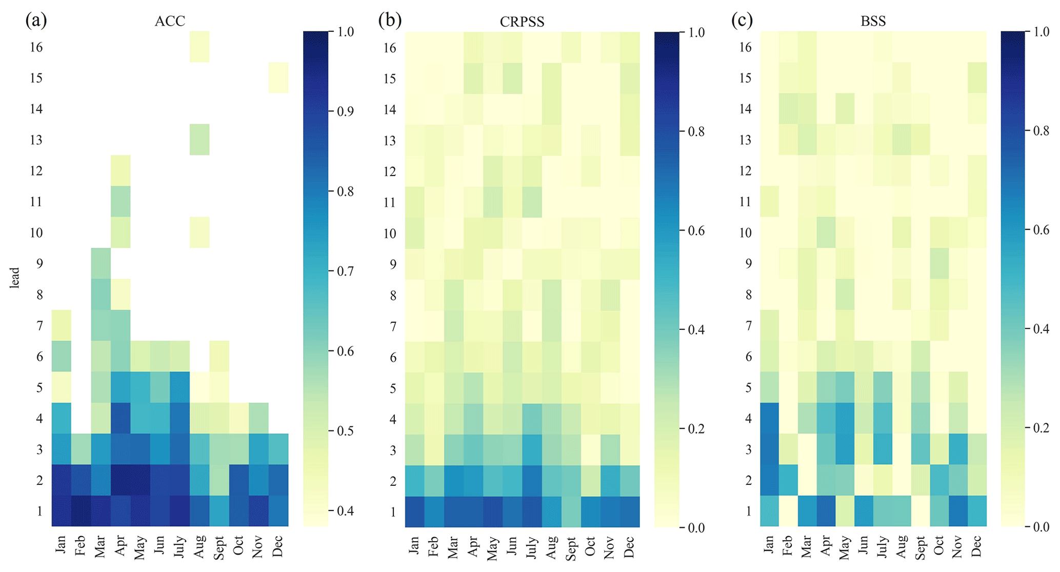
Figure 7 Heatmaps of weekly ACC (same as in Fig. 6), CRPSS, and BSS for discharge hindcasts (RF model) of the example station Hagenstein Boven for different initialization months. Cells in blue, for (a) ACC, (b) CRPSS and (c) BSS, indicate a good performance. For (b) CRPSS and (c) BSS, values above 0 indicate that the hybrid framework is outperforming the climatological reference.

3.2 Hydrological extremes – low flows

To assess the hindcast framework's capability to simulate low-flow events, the BSS was computed using a threshold for the lowest 20th percentile of discharge observations and hindcasts. This approach is similar to other studies using a threshold approach for drought definition (Van Hateren et al., 2019; Van Loon and Laaha, 2015). Figure 7 represents the weekly BSS in the right panel, again for the example station of Hagenstein Boven. Blue tiles on the heatmap indicate lead times where the hindcast framework outperforms the climatological reference strongly.

The BSS shows a less consistent skill pattern in the first lead month compared to the other scores. However, most of the skill that is seen shows a similar range of lead time, and the skill throughout long lead periods is decreased (e.g. after lead week 5). Compared to the other scores, tiles with lower BSS performance can be spotted in summer (June and August for longer lead times; September for the first lead month) and early spring months (February and March) for this station, in some cases for the first lead month or the following longer lead months. Some of these weeks appear to be more difficult to predict compared to early months in the year. This is likely due to unequal distribution of low-flow occurrences throughout the year, where, during summer months, low flows can be more common and therefore the chances of not fully capturing every event are higher; the low flows during winter are less common and are captured relatively well with the snowmelt dynamic, as seen in previous scores. However, important months in terms of capturing drought development (April and May) show skill for up to 5 weeks. The described observations for the example station are in line with findings at other stations along the Rhine river network and are less pronounced along the Meuse.

3.3 Difference between target variables and scenario runs

The result section so far has been focusing on the discharge hindcasts in order to be able to focus on the different evaluation scores in more detail. However, the hindcast framework was also used to hindcast surface water levels (Figs. B1–B4). Surface water level prediction skill for the national and model average (Fig. B1) show a slightly higher CRPSS skill than for discharge (Fig. 2). In addition, similar patterns and trends regarding ACC for stations along the main river network (Fig. B2) and CRPSS results (Fig. B3, for an example station) were observed. Yet, surface water levels seem to be more challenging to hindcast, with the evaluation scores being slightly lower, especially for stations in smaller channels, and further away from the main river network. Similar findings are found for BSS, where the performance of the hindcast for low flow periods was tested. As can be expected, stations which are not along the main river network and are located downstream of the main input variables (Rhine at Lobith; Meuse at Eijsden) show lower skills in capturing low flow periods compared to stations closer to input variables and the Rhine river. While ACC and BSS show a slightly lower performance, the CRPSS ranges are in the same range as for discharge hindcasts.

An additional discharge hindcast run was done, including water management information, to represent some of the major infrastructure, based on the same approach previously explored by Hauswirth et al. (2021). Similar to the findings in Sect. 3.1, only minor difference between the different ML methods were observed. Furthermore, incorporating the additional water management information only led to insignificant improvements regarding the hindcast skill. The improved performance and the differences in the ML model performance, as seen in the previous study by Hauswirth et al. (2021), could therefore not be detected in this forecasting experiment.

4 Discussion

In this study, we tested the suitability of ML models for seasonal predictions of several hydrological target variables at local scales throughout the Netherlands. This framework incorporated ML models over varying complexity, ranging from multilinear regression, lasso regression, and decision tree to random forests and LSTM random forest and long short-term memory model.

While the methods have shown differences in their performance during the training and testing phase on historical observations (especially their ability to reproduce extreme events; Hauswirth et al., 2021), interestingly, applying the same subset of models on seasonal (re)forecasting information did not lead to large differences in model performance. We hypothesize that this is caused by the large uncertainty in the meteorological and hydrological input data that outweighs the relative difference in performance by the different ML algorithms. In other words, the forecasting skill is very much dependent on the skill by which the input variables are forecasted, which apparently make the differences in skill between the ML models insignificant in comparison. In addition, the minor differences seen between the ML algorithms in the original hindcasts were further smoothed out while calculating the evaluation scores on different temporal scales. The results in this hindcast experiment and the minor differences between the methods that were observed can be interesting in terms of model choices, in case computational demand is a key factor. With simple methods showing similar performance to more complex ones, which require more time regarding set-up and training, the previous might appear more suitable. However, a more important factor limiting the model performance is the uncertainty introduced by incorporating seasonal (re)forecasting information. A subject for future research could be on how to incorporate and assess the way the different models deal with that additional challenge. Nevertheless, we observed that the ML modelling framework used here, which is based on locally trained models, allows for the opportunity to make hydrological forecasting more locally relevant by being able to forecast based on the station-specific characteristics.

While the ML models were previously trained on direct observations, the seasonal (re)forecasting information from SEAS5 and EFAS introduces additional uncertainty from their forecasting system. We deliberately decided not to retrain the ML models on the forecasting information, as this more closely mimics the normal operational setting in which an already-trained model is used to produce forecasts. However, this provides an additional challenge, as we add another source of potential uncertainty because the ML models might not be well tuned to the forecast information. Retraining the models would also open up the opportunity for the overfitting the ML models on the forecast data, which is something that should be avoided. Therefore, we preferred to use the more realistic operational scenario, and ML models trained on historic observations only, over a set-up that uses ML models specifically trained on forecast data. Assessing the approach of additionally retraining the models for different cases, e.g. focusing on extreme events or climate change trends, is an opportunity for future projects.

We extended our runs, including water management, in line with the approach previously explored by Hauswirth et al. (2021). However, incorporating variables that represent water management settings in the ML models led to negligible improvement, and the improved performance as seen in the previous study could not be detected. We think that the uncertainty included in the seasonal (re)forecast input data is having a larger influence than the one of added water management information, and therefore, the strength of incorporating the additional information as seen in the previous study could not be observed. For future research, it might be interesting to explore what additional steps would be beneficial in terms of model framework and data in order to also be able to capture and simulate the details of water management set-ups in a forecasting setting, as this would create the opportunity for scenario simulations.

The evaluation metrics show that, for hindcasts of discharge and surface water level stations initialized in the early spring, skilful predictions for the first lead month 1 can be made. For early spring and summer months, the skill increases up to 2–3 months, due to the snowmelt dynamic being captured by the models in their training phase and the presence of this signal in the seasonal reforecasts of the discharge at Lobith used as input to the ML models. The skilful prediction for the first few lead months is comparable with other studies which have evaluated physically based systems (Wanders et al., 2019; Arnal et al., 2018; Girons Lopez et al., 2021; Pechlivanidis et al., 2020). However, contrary to the large-scale physically based forecasting systems, hybrid frameworks such as the one presented in this study have been shown to skilfully forecast target variables at specific locations which would not be feasible and at a fraction of the computation demand. While training ML models can range from a few minutes to hours, depending on the method and set-up (Hauswirth et al., 2021), running the hybrid framework as used in this study only takes a few seconds to minutes per station and ensemble member. This can be interesting for water management needs at smaller scale or scenario analysis. Besides the fast running times of the models, an additional benefit for the current framework is the input data set, which can easily be replaced by other input sources regarding precipitation, evaporation, discharge, and surface water level as was done in this study with EFAS and SEAS5 data. It is, however, important to realize that the original computation time required for large-scale seasonal (re)forecasting information such as the latter two is still required but is outside of the hybrid framework presented here. However, in the case of scenario simulations, where local information would be required and tested in a more quick setting but based on one large-scale input data set, the hybrid framework is still of benefit as it can compute the different hindcasts more efficiently.

A further point to realize is that this framework only focuses on time series at existing stations and therefore does not address the challenge of predicting at ungauged basins. However, recent advances in deep learning methods show that forecasting at ungauged sites may be a possibility if auxiliary geographically distributed variables (elevation, soil, and river network topology) are incorporated (Kratzert et al., 2019).

Similar to Hunt et al. (2022), we show that a hybrid forecasting system can provide added benefits compared to physical forecasting system. In addition to Hunt et al. (2022), this work confirms that the benefits of hybrid forecasting can also be obtained for long-term forecasting. In this study, we also show that these hybrid forecasting systems have the ability to provide more local information compared to large-scale physically based systems. As with other models, using ML models in hydrology comes with benefits and drawbacks. While the data availability can be a limiting factor for effectively training a model, the flexibility and low computational demand compared to large-scale physically based models is an advantage. We think that, with the right data available, ML models like the ones used here can easily be (re)trained for more specific studies and cases as well. Additional training on low-flow periods, for example, could enhance drought predictions while incorporating climate change aspects, and land use could help to assess future trends regarding water availability under increased human influence.

5 Conclusions

In this study, we explored the suitability of a hybrid hindcasting framework, combining data-driven approaches and seasonal (re)forecasting information to predict hydrological variables locally for multiple stations at a national scale for the Netherlands. Different ML models, previously trained on historical observations, were run with a simple input data set based on forecast data from EFAS and SEAS5 and evaluated using the evaluation metrics anomaly correlation coefficient (ACC), continuous ranked probability (skill) score (CRPS and CRPSS), and brier skill score (BSS). The hindcast framework's skill was compared to the skill of a climatological reference hindcast. Aggregating the hindcasts of all stations and ML models revealed that the hindcasting framework was outperforming the climatological reference forecast by roughly 60 % and 80 % for discharge and surface water level hindcasts. ACC results further show that, independent of the discharge prediction's initialization month, a skilful prediction for the first lead month can be made. For spring months, the skill extends up to 2–3 months due to stronger link to snowmelt dynamics and temperature-related impacts on the hydrological cycle that were captured in the training phase of the model. CRPSS and BSS show a similar pattern of skilful predictions for the first few lead weeks compared to the climatological reference forecasts. Skilful discharge predictions are particularly observed along the main river networks, the Rhine and Meuse, which can be linked to the close proximity of the discharge input variables. This distribution of performance is also observed for surface water level hindcasts. We also observed that the difference between different ML models in the hindcast results are only minor, contrary to the differences observed when reproducing historical time series. This reduction in differences in performance between ML models is attributed to the relatively large uncertainties in seasonal (re)forecast data, reducing the relative impact of the model uncertainty in the total hindcast uncertainty. Even though the current hindcast framework is trained on historical observations, the hybrid framework used in this study shows similar skilful predictions to previous large-scale forecasting systems. With the focus on creating a hindcast framework that is simple in its set-up, fast, and also locally applicable, challenges that can come with large-scale operational forecasting systems for local users can be lowered. In addition, the ML hindcast framework also significantly reduces the computational demand and allows decision-makers to explore more options and better quantify forecast uncertainty using a variety of ML models and inputs. Adapting the framework to special interests, e.g. droughts or climate change trends, by retraining the original ML models for specifically this purpose could further increase its performance. We conclude that the ML framework, as developed in this study, provides a valuable way forward to making seasonal (re)forecast information more accessible to local and regional decision-makers in the field of operational water management. In this study, we purposely used publicly available seasonal forecast information which is globally available. This allows us to deploy this framework around the world and potentially provide relevant forecasting information for water managers and decision-makers outside of the study area.

Appendix A: Material and methods

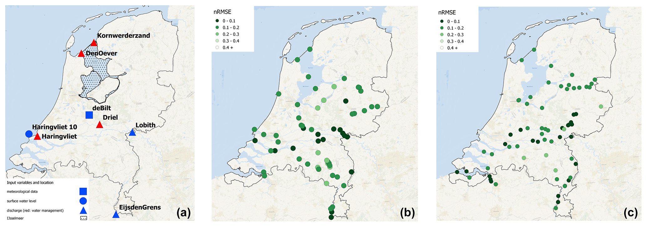
Figure A1 Overview input stations (a) for the ML model framework, the locations of discharge (b), and surface water level (c) target stations used during model development. All figures are directly taken from Hauswirth et al. (2021). Discharge and surface water level stations include the RMSE score achieved during evaluation of the modelling framework (more details can be found in Hauswirth et al., 2021). Maps were created using QGIS (QGIS Development Team, 2022), HCMGIS plugin and basemap data from Esri Ocean (Sources: Esri, GEBCO, NOAA, National Geographic, DeLorme, HERE, https://www.geonames.org (last access: March 2021), and other contributors), and the Global Administrative Areas (GADM) database.

Appendix B: Results

B1 General performance

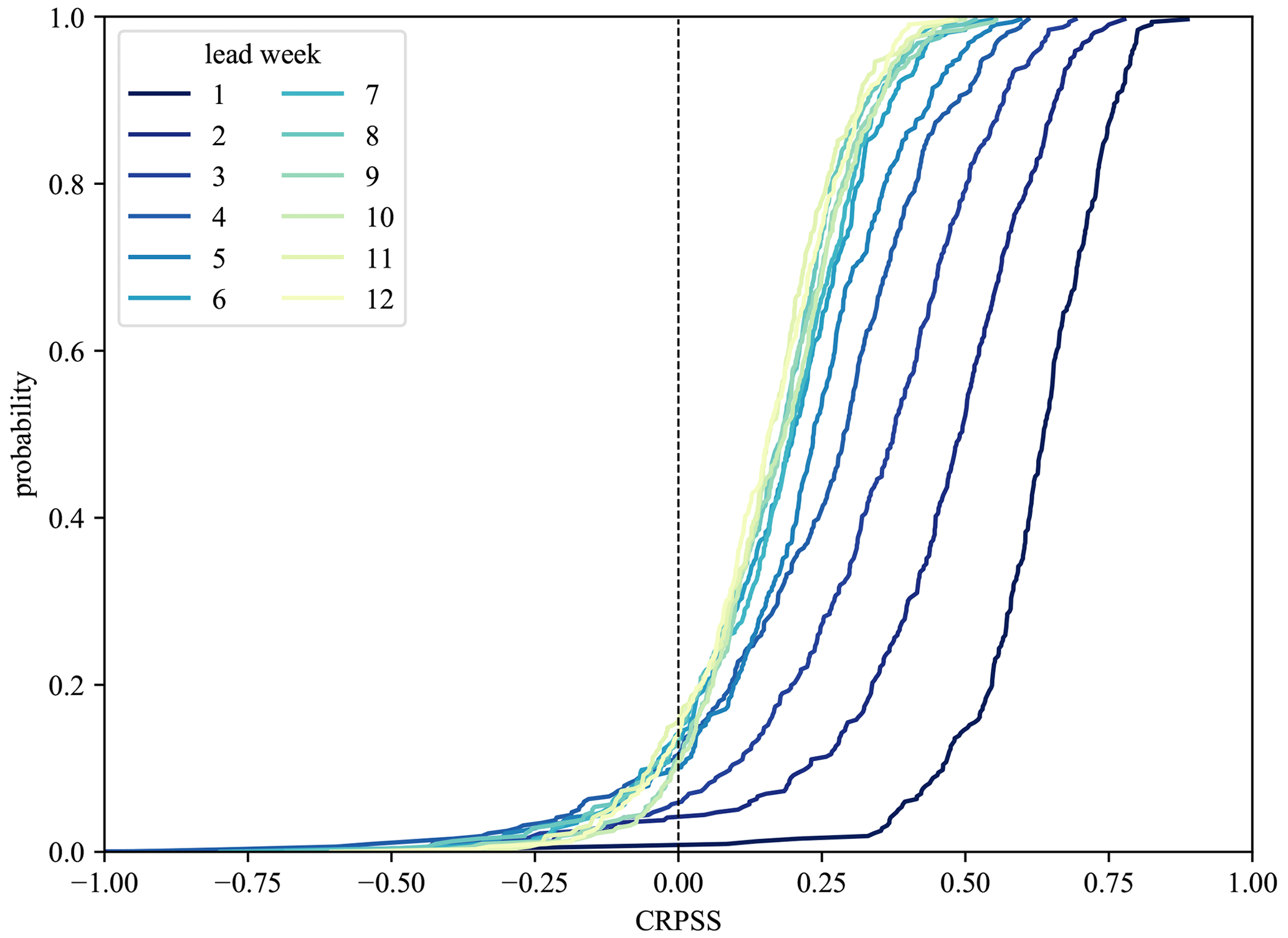
Figure B1 CDFs of weekly CRPSS shown for different lead weeks, with CRPSS being aggregated over all models and stations for fresh surface water level hindcasts (rivers, streams, and lakes).

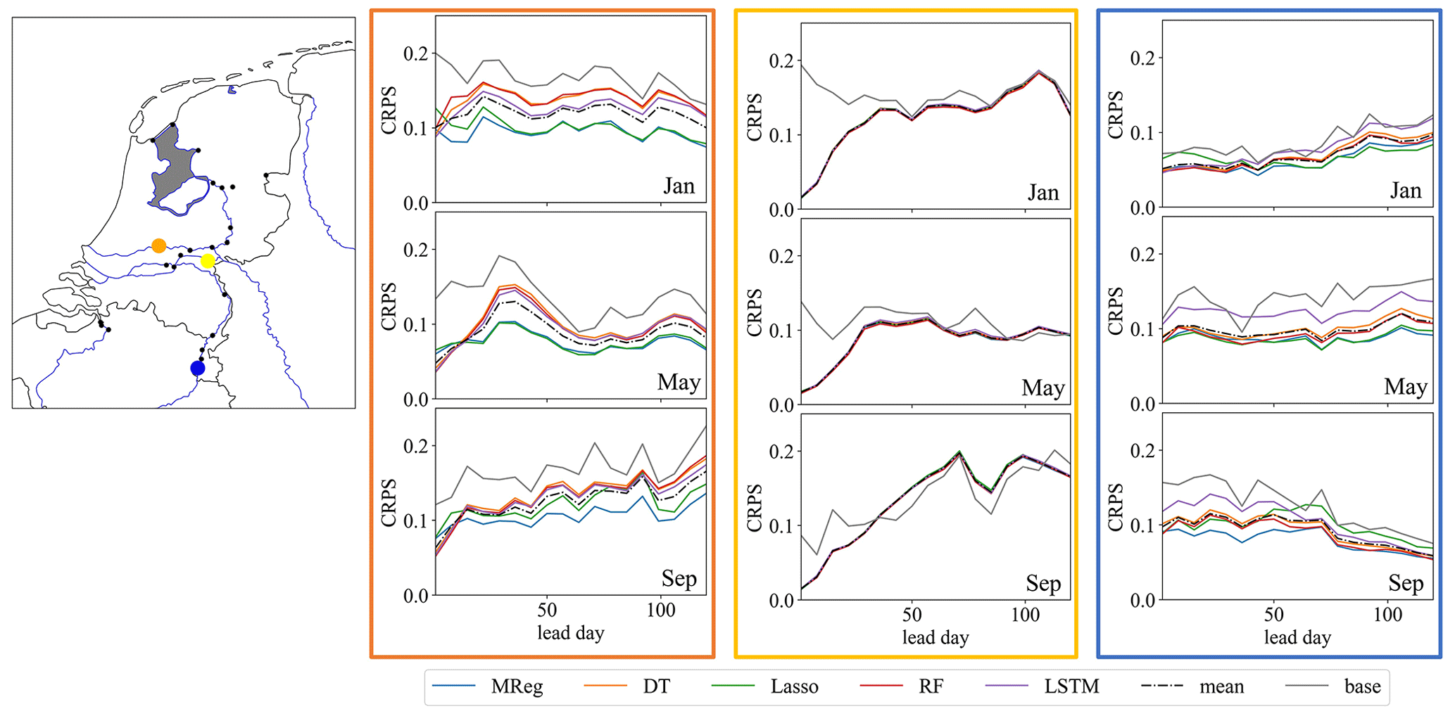
Figure B2 Overview of weekly CRPS scores for the months of January, May, and September. Different ML model scores, the average of the ML model score (dashed line), and climatological reference (grey) are shown for three surface water level stations along the main river networks – Hagenstein Boven (orange), Nijmegen Haven (yellow), and Borgharen Julianakanaal (blue). Maps were created using the Python package Cartopy (Elson et al., 2022), which uses basemap data made with Natural Earth and © OpenStreetMap contributors 2022. Distributed under the Open Data Commons Open Database License (ODbL) v1.0.

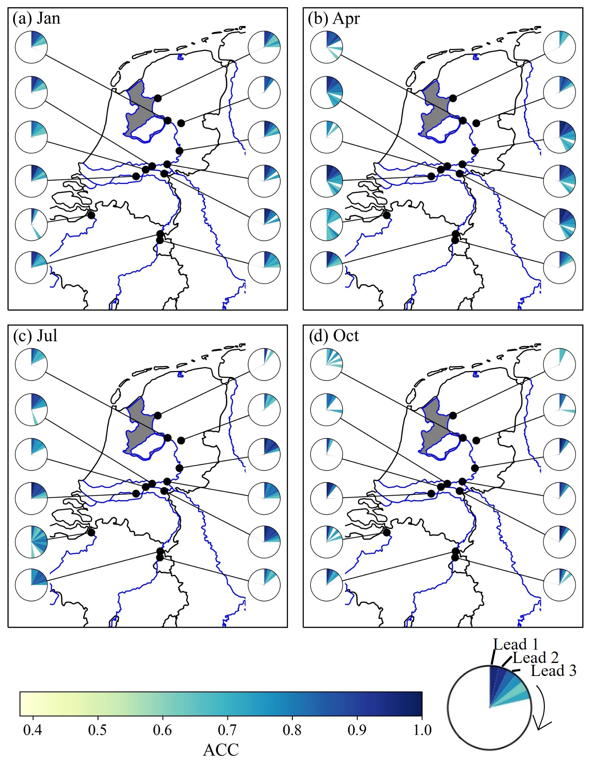
Figure B3 Anomaly correlation coefficient (ACC; weekly) for (a) January, (b) April, (c) July, and (d) October for surface water level hindcasts (fresh surface water levels such as rivers, streams, and lakes). Simulation results are based on the RF model showing the results for different stations (limited selection for visual purposes) in the national monitoring network. Only the major river networks are shown, and smaller streams or infrastructures are not highlighted (a station along the coast is placed at a sluice along a stream). Maps were created using the Python package Cartopy (Elson et al., 2022), which uses basemap data made with Natural Earth and © OpenStreetMap contributors 2022. Distributed under the Open Data Commons Open Database License (ODbL) v1.0.

Figure B4 Overview of the weekly evaluation scores for fresh surface water level hindcasts for different initialization months. (a) ACC, (b) CRPSS, and (c) BSS heatmaps for the example station of Nijmegen.