Atmospheric water transport connectivity within and between ocean basins and land

The global atmospheric water transport from the net evaporation to the net precipitation regions has been traced using Lagrangian trajectories. A matrix has been constructed by selecting various group of trajectories based on their surface starting (net evaporation) and ending (net precipitation) positions to show the connectivity of the 3-D atmospheric water transport within and between the three major ocean basins and the global landmass. The analysis reveals that a major portion of the net evaporated water precipitates back into the same region, namely 67 % for the Indian Ocean, 64 % for the Atlantic Ocean, 85 % for the Pacific Ocean and 72 % for the global landmass. It has also been calculated that 58 % of the net terrestrial precipitation was sourced from land evaporation. The net evaporation from the subtropical regions of the Indian, Atlantic and Pacific oceans is found to be the primary source of atmospheric water for precipitation over the Intertropical Convergence Zone (ITCZ) in the corresponding basins. The net evaporated waters from the subtropical and western Indian Ocean were traced as the source for precipitation over the South Asian and eastern African landmass, while Atlantic Ocean waters are responsible for rainfall over North Asia and western Africa. Atlantic storm tracks were identified as the carrier of atmospheric water that precipitates over Europe, while the Pacific storm tracks were responsible for North American, eastern Asian and Australian precipitation. The bulk of South and Central American precipitation is found to have its source in the tropical Atlantic Ocean. The land-to-land atmospheric water transport is pronounced over the Amazon basin, western coast of South America, Congo basin, northeastern Asia, Canada and Greenland. The ocean-to-land and land-to-ocean water transport through the atmosphere was computed to be 2×10⁹ and 1×10⁹ kg s⁻¹, respectively. The difference between them (net ocean-to-land transport), i.e. 1×10⁹ kg s⁻¹, is transported to land. This net transport is approximately the same as found in previous estimates which were calculated from the global surface water budget.

1 Introduction

The hydrologic cycle traces the continuous movement of the water in the Earth system. The atmospheric hydrological cycle starts from the evaporation regions and ends in the precipitation regions. Generally, evaporation tends to exceed precipitation over the ocean, while for land the opposite holds true. A consequence of this excess precipitation over land is that this surplus water eventually discharges into the ocean by the rivers, completing the atmospheric branch of the water cycle. The hydrological cycle is believed to strengthen in a future warmer climate. The Clausius–Clapeyron (CC) thermodynamic relation indicates that for every 1 ^∘C temperature rise, the saturation vapour pressure will approximately increase by 7 %. This implies that the vapour pressure, which is equivalent to the specific humidity or the amount of moisture in the atmosphere (Wallace and Hobbs, 2006), will also increase, as the tropospheric relative humidity is believed to remain the same in a warmer climate (Soden and Held, 2006). If the atmospheric circulation would remain unchanged, the water-vapour increase will solely act to intensify the moisture transport from the evaporation regions to the precipitation areas and help to magnify the strength of the existing global evaporation (E)–precipitation (P) patterns. This is the paradigm of “dry gets drier and wet gets wetter” or in other words “rich-get-richer mechanism” (Chou and Neelin, 2004). However, the increase of atmospheric moisture in a warmer climate does not necessarily imply that the global evaporation and precipitation will also increase by the same CC rate, as these are constrained by the surface energy budget (Held and Soden, 2006; Huntington, 2006). Analyses of future climate scenarios from Earth system models have revealed a 2–3 % increase in global precipitation per 1 ^∘C temperature rise (Allan et al., 2014). The imbalance between increasing rate of moisture and precipitation ensures that the precipitation intensity will increase in the future climate, while the frequency and duration are apt to decrease (Trenberth, 1999). In addition to this, the hydrologic cycle also plays a critical role in the global energy cycle through evaporative cooling of the Earth's surface and latent heating of the atmosphere. The impact of the hydrologic cycle is not only important for the atmosphere but also for the ocean. The evaporation-dominated regions over the ocean generally leads to high salinity and the precipitation-dominated regions to low salinity. The Atlantic Ocean is e.g. a net freshwater flux surplus ($E-P>\mathrm{0}$) region, in contrast to the Pacific Ocean where the opposite holds true. This in turn gives rise to a salinity asymmetry, which can explain the generation of deep water in the North Atlantic but not in the North Pacific Ocean (Warren, 1983; Broecker et al., 1985; Emile-Geay et al., 2003). The North Atlantic Deep Water (NADW) is an integral part of the Atlantic Meridional Overturning Circulation (AMOC), which distributes heat within the climate system (Vellinga and Wood, 2008). It is projected by many climate models that the AMOC will weaken during the 21st century, which could be linked to changes in the hydrologic cycle (Stocker et al., 2014).

Given these diverse roles of the hydrologic cycle within the Earth system, it is important to disentangle and understand its different parts. Previous studies were able to provide an estimate of the water storage in the reservoirs and also the net exchange of water between them using the surface water budgets (Chahine, 1992; Trenberth et al., 2007, 2011; Rodell et al., 2015). The atmospheric water transport between the global ocean and land, the two dominating water reservoirs, are primarily obtained by integrating the net freshwater flux (E−P) over them. The integrated E−P over the ocean is positive and calculated to be approximately 1 Sverdrups (1 Sv ≡ 10⁹ kg s${}^{-\mathrm{1}}=\mathrm{31}\mathrm{536}$ km³ yr⁻¹, assuming water density is constant at 1000 kg m⁻³), which is transported to land (Schmitt, 2008). Due to water-mass conservation, this 1 Sv is equivalent to the negative E−P integral over land (as P>E over the land), and will return to the ocean through river discharges. The E−P can either be directly obtained from the observationally based reanalysis data sets or derived from the moisture budget analysis (Trenberth et al., 2011). These kinds of studies suffer from the limitation that they cannot provide information about the atmospheric water transport within and between different ocean basins and land. In addition, knowledge about how much of the ocean/land evaporated water precipitates over the ocean/land itself and is transported to the land/ocean is not achievable. However, these questions will be possible to address using Eulerian/Lagrangian atmospheric water tracing schemes (Van der Ent et al., 2010; Tuinenburg et al., 2020; Stohl and James, 2004; Stein et al., 2015; Dey and Döös, 2020). A list of atmospheric water tracing models and their advantages and disadvantages has been discussed briefly in Dominguez et al. (2020). The primary objective of the present study is to link 3-D atmospheric water transports within and between different ocean basins and land using Lagrangian trajectories, which makes it possible to trace water from the net evaporation at the surface to where it precipitates. This will facilitate the construction of an atmospheric freshwater connectivity matrix, which will provide both quantitative as well as qualitative descriptions of the 3-D atmospheric water exchange.

2 Methods and data

2.1 Lagrangian model for tracing water in the atmosphere

The mass conserving Lagrangian trajectory model TRACMASS v7.0 (Aldama-Campino et al., 2020; Döös, 1995) was used in the present study to obtain a detailed understanding of the global hydrologic cycle. One of the unique characteristics of TRACMASS is that it uses mass transports through the model grid box faces instead of velocity fields (Vries and Döös, 2001). TRACMASS was employed frequently to track the oceanic water-transport pathways (Berglund et al., 2017, 2021; Döös et al., 2008) and atmospheric air-mass routes (Kjellsson and Döös, 2012). In Dey and Döös (2020), TRACMASS was updated in order to trace water instead of air in the atmosphere. The atmospheric water tracing version of TRACMASS was also implemented recently to study the seasonal and interannual characteristics of the South Asian summer monsoon precipitation (Dey and Döös, 2021). Note here that these trajectory calculations are based on atmospheric water-mass transport in kg s⁻¹ and not transports of humid air. We are hence tracing the actual atmospheric water and not the moisture change along air-parcel trajectories. An elaborate evaluation of the atmospheric and oceanic trajectory schemes that are used in TRACMASS can be found in Döös et al. (2017).

The horizontal water transports through the model grid box faces are obtained by multiplying the air transports with its water content. The vertical water transport field is then obtained from an atmospheric water-mass conservation equation (Dey and Döös, 2019), which is zero at the top of the atmosphere and equal to E−P at each model level. The calculation of the vertical water transport from the conservation equation confirms that the evaporation, precipitation, condensation and advection of moisture by the winds are all summed up as the vertical water transport and cannot be separable. Note that the diffusive water transports, specific rain water and snow water content were omitted in Dey and Döös (2019, 2020) and in the present study due to its unavailability from the ERA-Interim, but could be included in future studies. For a detailed mathematical derivation of the atmospheric water transport, see Dey and Döös (2019, 2020, 2021).

The mass conserving ability of TRACMASS (i.e. mass transport of a trajectory is conserved throughout its journey) has made it possible to compute Lagrangian stream functions from the simulated trajectories. The Lagrangian stream function is a useful tool to understand atmospheric and oceanic circulation pathways and has been used in previous studies extensively (Blanke et al., 1999; Berglund et al., 2017; Kjellsson and Döös, 2012; Döös et al., 2008). In the present study, the Lagrangian meridional and zonal overturning stream functions were computed to quantify atmospheric water-mass transport pathways in the meridional–vertical and zonal–vertical coordinate system, respectively. The Lagrangian meridional overturning stream function can be expressed as

$$\begin{array}{}\text{(1)}& {\mathit{\psi }}_{j,k}=\sum _{k^{\prime }=k}^{kz}\sum _i\sum _m{T}_{i,j,k^{\prime },m}^y.\end{array}$$

Here, i, j and k^′ are the zonal, meridional and vertical coordinates through which the trajectory indexed m passes. $T_{i,j,k^{\prime },m}^y$ is the atmospheric water transport (kg s⁻¹) by the trajectory indexed m through the zonal–vertical grid box. The highest vertical level of the atmosphere is at 0.1 hPa and denoted as $k^{\prime }=kz$. Note that the stream lines will be open and crossing the surface due to the sources (net evaporation) and sinks (net precipitation) of atmospheric water. Similarly, the Lagrangian zonal overturning stream function was computed as

$$\begin{array}{}\text{(2)}& {\mathit{\psi }}_{i,k}=\sum _{k^{\prime }=k}^{kz}\sum _j\sum _m{T}_{i,j,k^{\prime },m}^x,\end{array}$$

where $T_{i,j,k^{\prime },m}^x$ is the Lagrangian water transport (kg s⁻¹) through the meridional–vertical grid box face. The vertically integrated zonal ($F_{i,j}^x$) and meridional ($F_{i,j}^y$) water flux was computed from the 3-D simulated water trajectories to describe atmospheric water transport pathways in longitude–latitude framework as follows:

$$\begin{array}{}\text{(3)}& F_{i,j}^x={\displaystyle \frac{\sum _{k^{\prime }=\mathrm{0}}^{kz}\sum _m{T}_{i,j,k^{\prime },m}^x}{\mathrm{\Delta }{y}_{i,j}}},\end{array}$$

$$\begin{array}{}\text{(4)}& F_{i,j}^y={\displaystyle \frac{\sum _{k^{\prime }=\mathrm{0}}^{kz}\sum _m{T}_{i,j,k^{\prime },m}^y}{\mathrm{\Delta }{x}_{i,j}}}.\end{array}$$

The longitudinal and latitudinal grid spacing is denoted as Δx and Δy, respectively. The resultant of the vertically integrated horizontal water flux is thus

$$\begin{array}{}\text{(5)}& F_{i,j}=\sqrt{{\left(F_{i,j}^x\right)}^{\mathrm{2}}+{\left(F_{i,j}^y\right)}^{\mathrm{2}}},\end{array}$$

which has the unit Sv m⁻¹ (1 Sv ≡ 10⁹ kg s⁻¹). The calculated water trajectories were also used to compute atmospheric water residence time (τ_i,j) following Dey and Döös (2020, 2021) as

$$\begin{array}{}\text{(6)}& {\mathit{\tau }}_{i,j}={\displaystyle \frac{\sum _{m=\mathrm{1}}^M\left\{\left(t_m^{\mathrm{P}}-t_m^{\mathrm{E}}\right)\cdot T_{i,j,m}^z\right\}}{\sum _{m=\mathrm{1}}^M{T}_{i,j,m}^z}},\end{array}$$

which is the lifetime of the atmospheric water between net evaporation and net precipitation. Here, $T_{i,j,m}^z$ is the water transport of the trajectory indexed m through the surface. M is the total number of trajectories, and t^P and t^E is the time when the atmospheric water trajectories precipitate and evaporate, respectively.

2.2 Data source

The atmospheric water transports were computed using the surface pressure, specific humidity, specific cloud liquid and ice water content and horizontal wind velocities from the ERA-Interim reanalysis (Dee et al., 2011). The inclusion of the specific cloud liquid and ice water content in the water transport calculation is an update as compared to Dey and Döös (2020, 2021). The data sets were obtained for the years 2016 and 2017 with 0.75^∘ spatial resolution, 6-hourly temporal resolution and 60 hybrid vertical model levels. It is noteworthy that to satisfy the mass conservation property of the Lagrangian model, TRACMASS requires data at model levels and not at interpolated pressure levels (Dey and Döös, 2021).

Figure 1 Spaghetti plot of few selected atmospheric water trajectories for the month of January 2016. The selected ocean basins are represented by different shadings of gray and defined as the Indian Ocean (IO), Pacific Ocean (PO) and Atlantic Ocean (AO). Note that the Arctic Ocean is included in the Atlantic. The global landmass is taken as one single entity. The atmospheric water transport within and between the ocean basins and land has been calculated based on these defined sectors. The representative trajectories associated with these intra- and inter-basin water transport are labelled with different colours. The black dots indicate the starting points and the red points represent the ending points of the atmospheric water trajectories.

2.3 Lagrangian study configuration

To understand the 3-D global atmospheric water transport, the Lagrangian trajectories were started over the entire surface of the globe when evaporation exceeded precipitation, and followed until they reach back to the surface, which occurs when precipitation exceeded evaporation. These water trajectories were started at the surface every 6 h during 2016, where E>P, then advected by the 3-D mass transport of water and followed until they reached back to the surface, where P>E. In total, more than 89 million water trajectories were started with more than 7 million trajectories each month. The position of a given atmospheric water trajectory within a grid box is solved analytically in space and with a stepwise-stationary scheme (Döös et al., 2017) in time. The trajectories were integrated in time with six intermediate time steps between each 6-hourly output data from the ERA-Interim. The trajectories were, however, followed for a maximum of 1 year. Only 0.4 % remained in the atmosphere after 1 year, and were subsequently discarded. The 3-D atmospheric water transport connection within and between different ocean basins and land, which can be regarded as an atmospheric water connectivity matrix, was estimated by sorting different classes of atmospheric trajectories based on their starting (net evaporation) and ending (net precipitation) positions. In the present study, the starting and ending points of the water trajectories were classified into the global landmass and the three major ocean basins, as defined in Fig. 1. The ocean basins are termed the Indian, Pacific and the Atlantic Ocean (including the Arctic ocean).

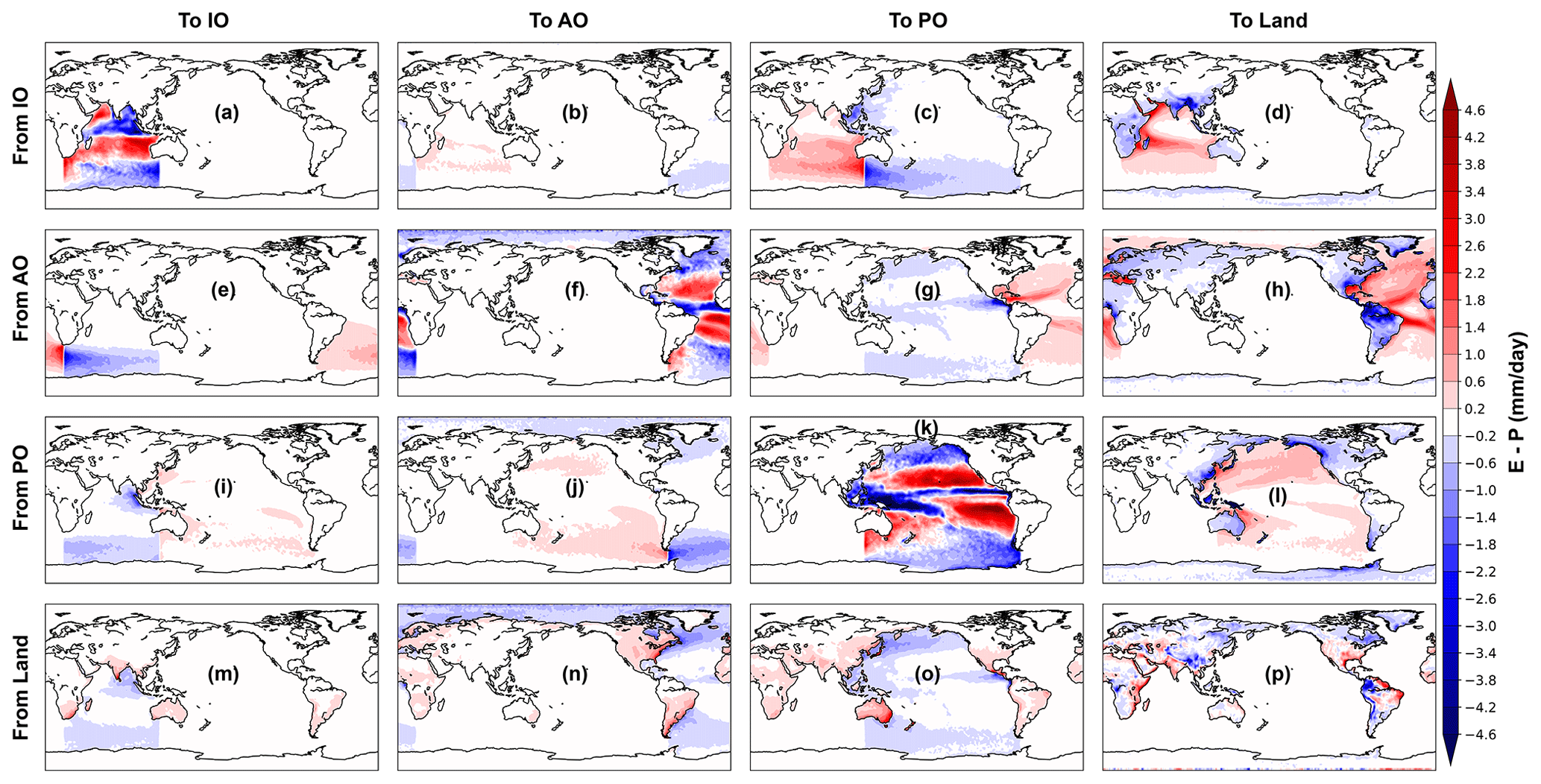
Figure 2 Annual mean E−P (mm d⁻¹) inferred from the atmospheric waters travelling from the surface net evaporative regions (red contours) to the net precipitation areas (blue contours). The rows represent the net evaporative (starting points of the atmospheric water trajectories) sectors and the columns represent the net precipitation (ending points of the trajectories) regions.

3 Results

3.1 Atmospheric water connectivity

The atmospheric water is always on the move through space and in time within the climate system. In order to grasp the full characteristics of the atmospheric water circulation, it is thus necessary to reduce its dimensionality. The geographical connection of the atmospheric water transports within and between the ocean basins and the global landmass has been established by tracing the atmospheric water from the evaporation-dominated to the precipitation-dominated regions (Fig. 2), which are the starting and ending points of the trajectories. Additionally, a quantitative view of this geographical atmospheric water transport connection is presented in Table 1 by integrating the net evaporation/precipitation transport obtained from the sorted classes of trajectories. This integration of either net evaporation or precipitation will give the same result due to the mass-conserving property of the Lagrangian model TRACMASS. The atmospheric water movement in the horizontal–vertical plane is obtained by calculating the Lagrangian overturning water-mass stream functions using Eqs. (1) and (2), and presented in latitude–pressure and longitude–pressure coordinate systems (Figs. 3 and 4, respectively). In addition, vertically integrated horizontal water flux computation (using Eq. 5) is used to describe the water transport routes in longitude–latitude framework (Fig. 5). Note that the stream lines represent the integrated atmospheric water transport routes and is based on the sum of the Lagrangian trajectories, which should not be confused with the paths of the individual trajectories. Additionally, the stream lines start at the surface when E>P and terminate where the opposite holds true. While interpreting the atmospheric water pathways from the meridional and zonal overturning stream functions, it should be remembered that these are zonally and meridionally integrated pathways, respectively. For instance, the atmospheric water mass crossing a longitude can be transported zonally both by the tropical easterly trade winds and by the mid-latitude westerlies. If e.g. the westerlies transport more water than the easterlies at the same longitude, then the meridionally integrated zonal overturning stream function will only show the dominant westerly signal. The residence time of the atmospheric water was mapped geographically at the net evaporation points using Eq. (6). This mapping was split up using the connectivity matrix so that the residence times indicate the inter- and intra-basin transport timescales (Fig. 6). This residence time was calculated at the points where net evaporation exceeds a monthly mean value of 0.2 mm d⁻¹, in order to focus on the main source regions of the atmospheric water.

Figure 3 The Lagrangian meridional overturning stream function within and between the ocean basins and land. This has been undertaken by grouping the trajectories according to their starting and ending locations. The starting and ending points of the atmospheric trajectories are defined as per the sectors presented in Fig. 1. Note that the stream lines represent the integrated atmospheric water transport routes and is based on the sum of the Lagrangian trajectories, which should not be confused with the paths of the individual trajectories.

Table 1 Atmospheric freshwater transport within and between the ocean basins and land. The rows represent net evaporative (atmospheric water source) sectors and the columns represent the net precipitation (atmospheric water sink) regions. Units are in Sv (≡10⁹ kg s⁻¹). The percentages in the parentheses represent fractions of the net evaporation that are transported from the source region.

Figure 4 Same as Fig. 3, but for the zonal overturning stream function.

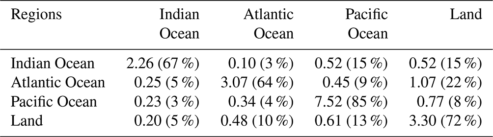
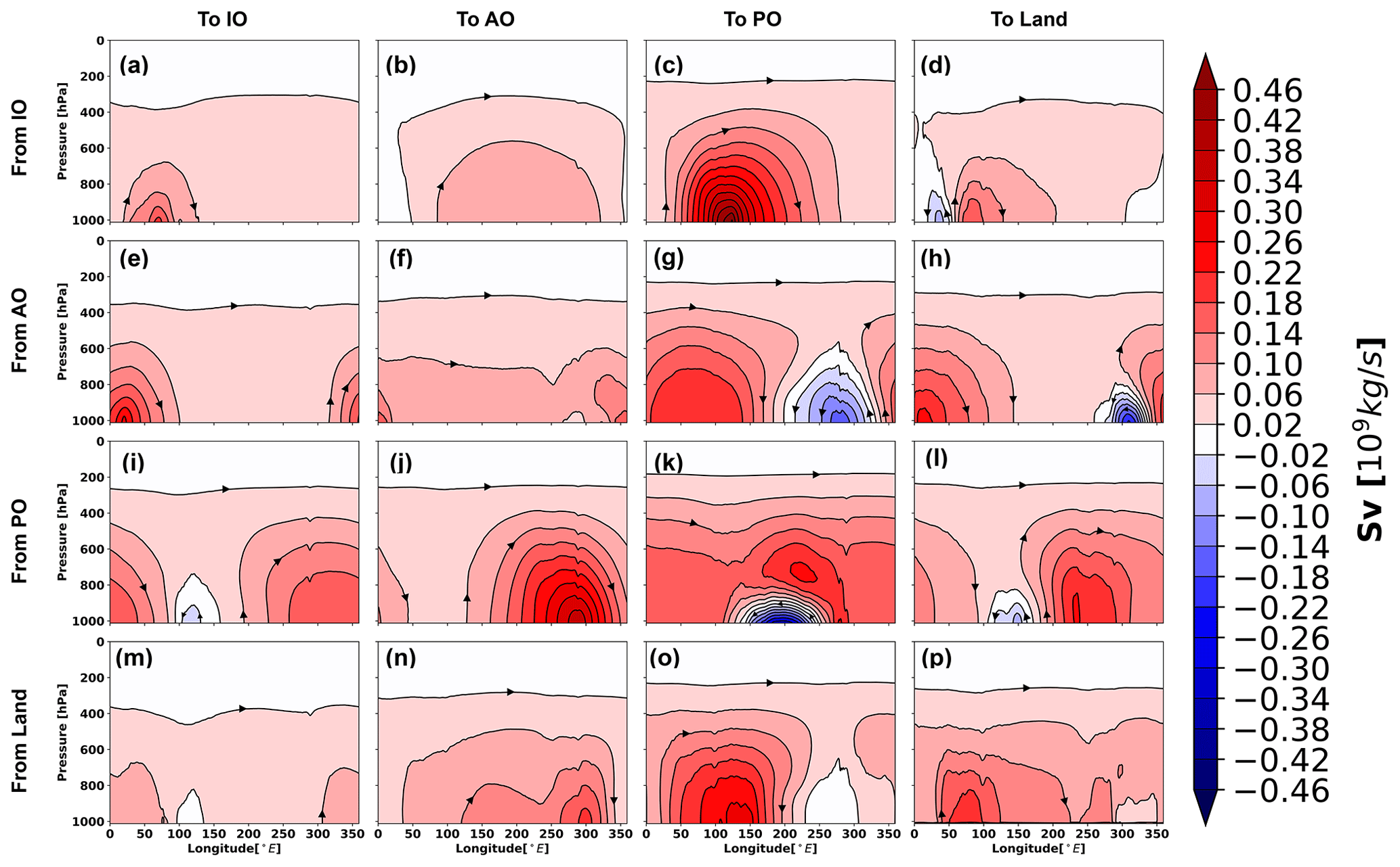
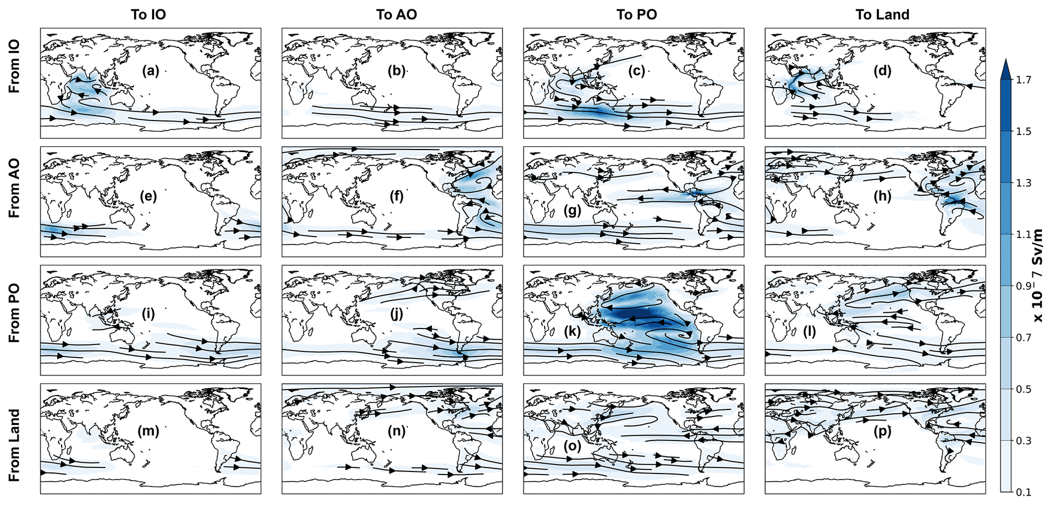
Figure 5 The vertically integrated horizontal water flux (shaded; Sv m⁻¹) within and between the ocean basins and land. This has been achieved by grouping the atmospheric water trajectories according to their starting and ending locations. The starting and ending points of the Lagrangian trajectories are defined as per the sectors presented in Fig. 1. The flux directions are given by the black lines.

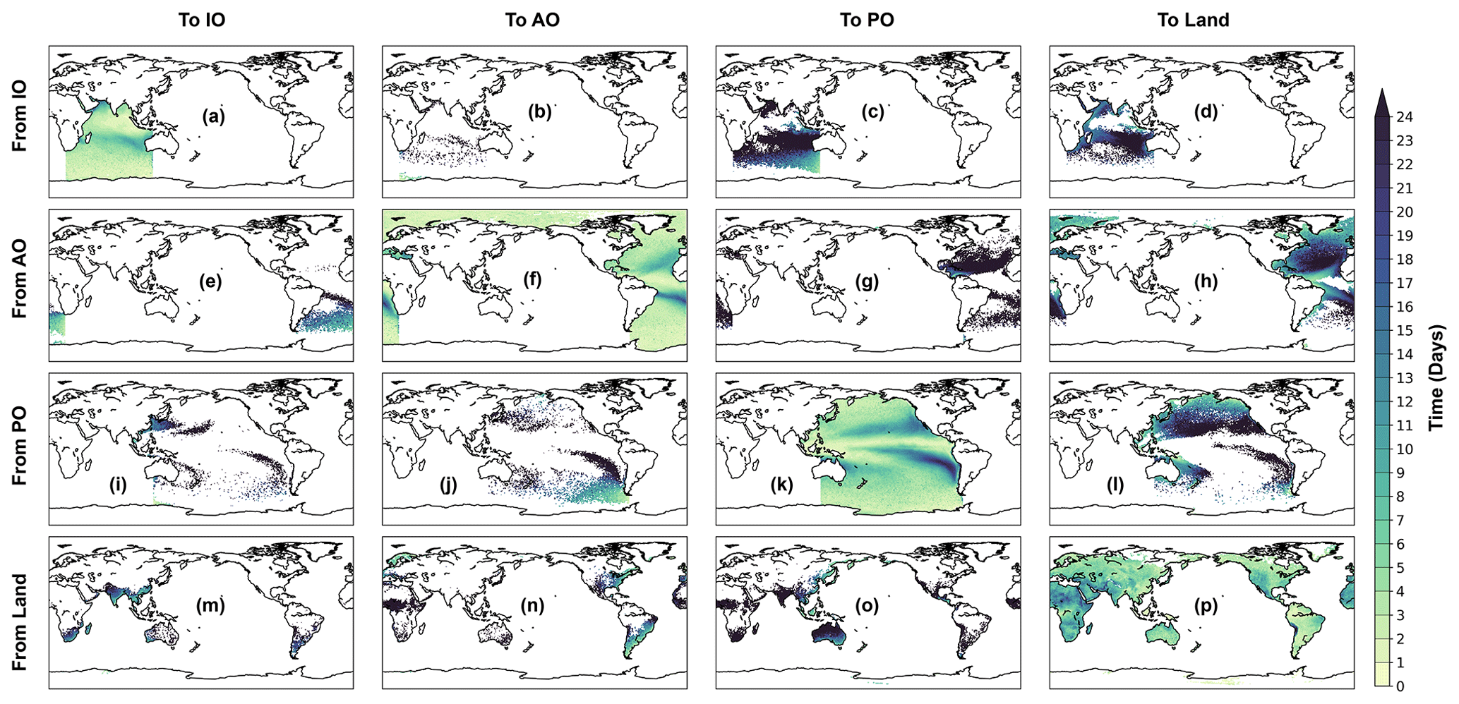
Figure 6 The average residence time (days) of the atmospheric waters mapped on their net evaporative points within and between the three ocean basins and land. Note that this has been mapped where the net evaporation exceeds a monthly mean value of 0.2 mm d⁻¹. The residence time has been calculated from the time the trajectories have spent in the atmosphere between their starting (net evaporation) and ending (net precipitation) points.

The results show that the net evaporation from the subtropical Atlantic, Pacific and Indian Ocean is the major source of water for net precipitation over the Intertropical Convergence Zone (ITCZ) in their respective basins (Fig. 2a, f and k). A major portion of the net evaporated water from the ocean basins was found to precipitate over their source sectors (Table 1). On an annual average, 67 % (2.26 Sv), 64 % (3.07 Sv) and 85 % (7.52 Sv) of the net evaporation from the Indian, Atlantic and Pacific Ocean precipitates over the same oceanic basin (Table 1). The meridional overturning stream function and vertically integrated horizontal water transport corresponding to these intra-basin atmospheric water transports (Fig. 3a; 5a, 3f; 5f and 3k; 5k) show that the Equatorward meridional transport in the Atlantic and the Pacific oceans and northward transport in the Indian Ocean are dynamically responsible for most of the oceanic ITCZ rainfall. The easterly (east to west) water transport within the Pacific Ocean (blue cell in Fig. 4k and black lines in Fig. 5k) also plays a crucial role for the Pacific ITCZ precipitation and shows the atmospheric water movement within the Walker circulation. The evaporative waters from the Indian, Atlantic and Pacific oceans stay on an average 4, 3 and 5 d, respectively, in the atmosphere before precipitating back into their basins of origin (Fig. 6a, f and k). Note that the residence time map has a large spectrum of values and varies a lot within small distances in some of the defined regions, e.g. the evaporative water from the subtropical Pacific Ocean has residence time from 0 d to more than 24 d (Fig. 6k). The rainfall over the South Asian landmass and eastern Africa is traced to originating and transporting mostly from the subtropical and western Indian Ocean (Figs. 2d and 5d). Note that this is an annual mean figure and consists of precipitation signals from the entire year. The atmospheric water transport from the Indian Ocean to the landmass is estimated to be around 0.52 Sv, which is 15 % of the total Indian Ocean net evaporation (Table 1). The evaporated water from the Indian Ocean is primarily transported by the Somali low-level jet to the South Asian landmass. This low-level jet is a southwesterly flow which is active along the Somali coast during the summer monsoon months of June to September. The atmospheric water transport pathways associated with this jet is captured by the meridional and zonal overturning stream functions (Figs. 3d and 4d), in which the northward (Fig. 3d) and eastward (Fig. 4d) flow components carry atmospheric water to South Asia. Additionally, the horizontal water transport pathway from the Indian Ocean to the South Asian landmass by the Somali low-level jet is clearly noticeable in Fig. 5d.

The easterly (Figs. 4d and 5d) component of the flow field transports water to eastern Africa from the nearby Indian Ocean. The water that evaporated from the Indian Ocean and transported to land remains around 20 d in the atmosphere (Fig. 6d). The transport from the subtropical Atlantic Ocean to the tropical and mid-latitude Pacific Ocean (Fig. 2g) is found to be accomplished by the easterly and westerly winds, respectively (Figs. 4g and 5g), and is calculated to be approximately 0.45 Sv (Table 1). The mean residence time of the evaporated waters from the Atlantic Ocean that are transported to the Pacific Ocean is 35 d (Fig. 6g). The majority of the South and Central American precipitation is found to be transported from the tropical Atlantic (Fig. 2h) with the help of easterly trade winds (blue cell in Fig. 4h and black lines in Fig. 5h). The Atlantic storm tracks, which orientated in an eastward direction, seemed to be responsible for the European and North Asian precipitation (Figs. 2h, 4h and 5h). The annual mean western African precipitation that is dominated by the western African monsoon is traced to originating from the Atlantic Ocean and moves eastward (Figs. 2h and 4h). The winds over the Atlantic Ocean transport around 1.07 Sv atmospheric water to the land, which is 22 % of its net evaporation (Table 1). The Atlantic Ocean evaporated waters stay in the atmosphere for 15 d before precipitating over land (Fig. 6h). The rainfall over the west coast of North America and eastern coasts of Asia and Australia is primarily sourced from the Pacific Ocean (Fig. 2l), and its pattern closely resembles the pathways of the Pacific storm tracks. The total atmospheric water transport from the Pacific Ocean to the landmass is approximately 0.77 Sv (Table 1). The average residence time of the waters that are evaporated from the Pacific Ocean and precipitated over the landmass is found to be 21 d (Fig. 6l). The land-to-land atmospheric water transport is prominent over the Amazon basin, western coast of South America, Congo basin, the northeastern sector of Asia, Canada and Greenland (Fig. 2p). The total amount of land-to-land atmospheric water transport is estimated to be around 3.30 Sv and is equal to 72 % of its evapotranspiration, while 58 % of the terrestrial precipitation was sourced from the land evaporation (Table 1). The evaporated water from land that falls back over the continents spends 6 d in the atmosphere (Fig. 6p). A spatial view of the global atmospheric water residence time (mapped at the evaporation and precipitation points) has been constructed from the Lagrangian water trajectories (Fig. S1 in the Supplement) and discussed in Sect. S1 in the Supplement. The global average residence time of the atmospheric waters is calculated (using Eq. 6) to be 9 d, which is similar to the estimate of 8 to 10 d by van der Ent and Tuinenburg (2017) and the references therein.

3.2 A simplified quantitative view of the atmospheric water cycle

A simplified schematic of the annual mean global atmospheric water transports from both the surface water budget and Lagrangian perspectives is presented in Fig. 7. It reflects the advantage of using a Lagrangian framework, from which ocean-to-ocean, ocean-to-land, land-to-land and land-to-ocean atmospheric water transport could be and was calculated (Fig. 7, bottom). The sketch was constructed by summing and rounding off the values of Table 1. For instance, net evaporation over the entire ocean was calculated by summing all the values of the atmospheric water transports from the defined ocean basins. The net evaporative transport from all the ocean basins is around 17 Sv, of which nearly 16 Sv precipitates over the ocean itself. The net ocean-to-land transport is thus 1 Sv, which returns to the ocean as runoff from land, and equals the difference between the land net evaporation (≈4.6 Sv) and land net precipitation (≈5.6 Sv). It is found that 88 % of the oceanic net evaporation (i.e. approximately 15 Sv) is transported back to the ocean through precipitation. The ocean-to-land transport is computed to be around 2 Sv, while the land-to-ocean atmospheric water transport is approximately 1 Sv. The difference between them (i.e. 1 Sv) is the same as the net ocean-to-land water transport through the atmosphere one might obtain from an atmospheric surface water budget point of view. The net land evapotranspiration is calculated to be around 4.6 Sv, and 72 % of this (i.e. around 3.3 Sv) goes into terrestrial precipitation. This estimate is similar to the estimate of 70 % by Tuinenburg et al. (2020), which was based on the higher resolution ERA5 atmospheric reanalysis data during 2008–2017 and a trajectory-based moisture tracing model UTrack. However, Link et al. (2020) and Van der Ent et al. (2010) reported a lower estimate of around 59 % and 57 %, respectively, while using the Eulerian numerical moisture tracking model Water Accounting Model (WAM), coarser ERA-Interim data and different study period. The net land precipitation is estimated around 5.6 Sv, and 58 % of this (i.e. approximately 3.3 Sv) is found to originate from the land evaporation. This estimation is comparable with the Tuinenburg et al. (2020) study in which they noted that 51 % of the global precipitation has evaporated from land. A study by Van der Ent et al. (2010) using WAM-1layer model and ERA-Interim reanalysis product reported that the continental precipitation recycling is 40 %, an estimate lower than the present study. However using an updated moisture tracking model WAM-2layers and land evaporative fluxes from the Simple Terrestrial Evaporation to Atmosphere Model (STEAM), van der Ent et al. (2014) found that the continental precipitation recycling dropped to 36 %.

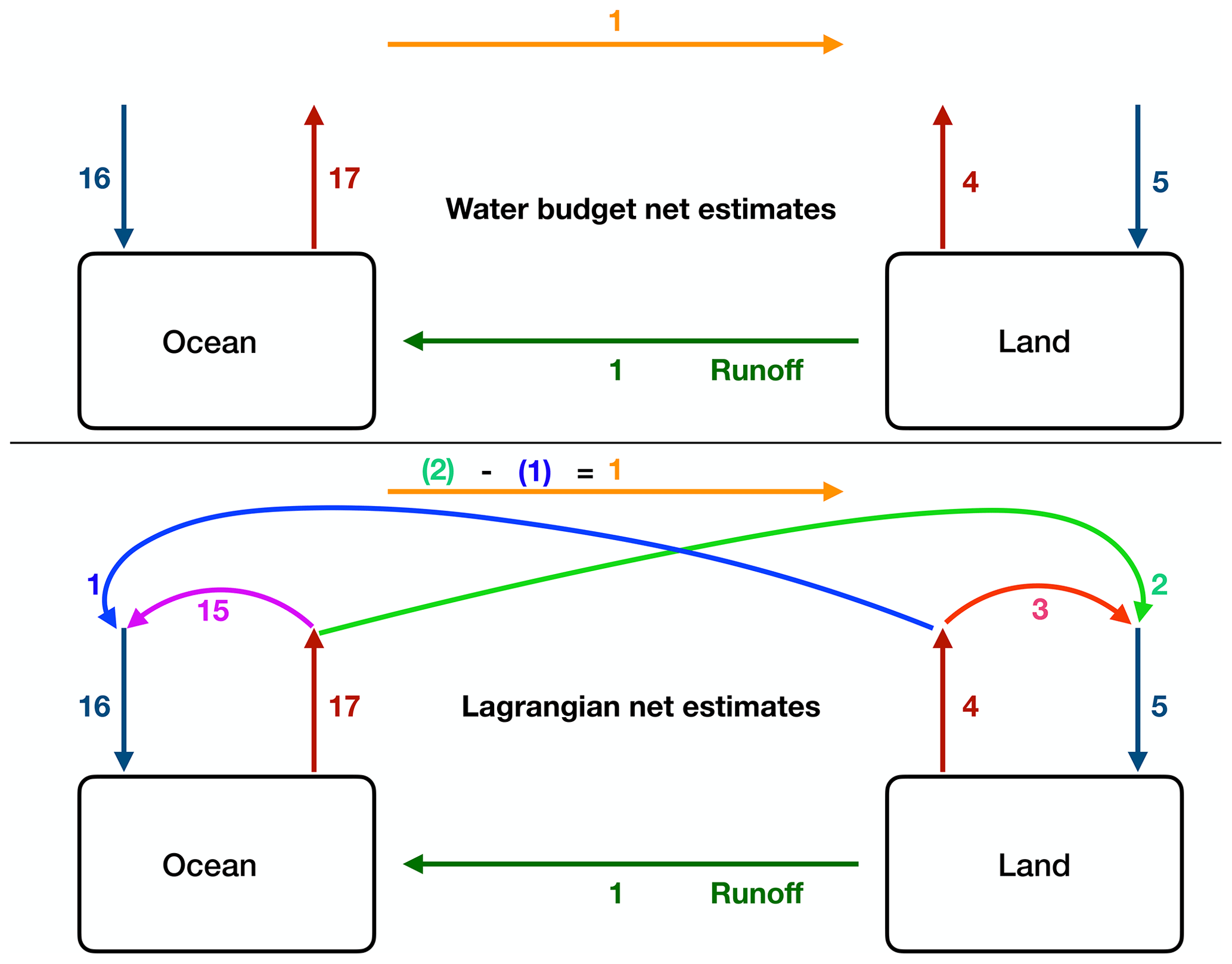
Figure 7 A sketch of the atmospheric water exchange between the global ocean and land. The top panel shows the surface water budget understanding of the hydrologic cycle, while the bottom panel elaborates the intricacies of the water movement that can be obtained using a Lagrangian framework. The upward and downward arrows represent net evaporation and net precipitation transport, respectively. Note, the numbers presented here are the crudely estimated transports from Table 1 and have not been used for any quantification. Units are in Sverdrups (1 Sv ≡ 10⁹ kg s⁻¹). It is important to mention that the net evaporation and net precipitation transports presented here are higher (with different magnitudes) than the previous estimates such as Trenberth et al. (2007) and Chahine (1992), and it might be due to the way E−P has been computed in the present study which omits diffusive atmospheric water transport and time correlations.

3.3 Limitations

The strength of the hydrological cycle in the present study is stronger than previous estimates such as Chahine (1992), Trenberth et al. (2007), Rodell et al. (2015) and others. For instance, the total global ocean evaporation was reported to be 413×10³ km³ yr⁻¹ in Trenberth et al. (2007), 434×10³ km³ yr⁻¹ in Chahine (1992), $\mathrm{449.5}\pm \mathrm{22.2}\times {\mathrm{10}}^{\mathrm{3}}$ km³ yr⁻¹ in Rodell et al. (2015), 460×10³ km³ yr⁻¹ in van der Ent and Tuinenburg (2017), and in the current study the net evaporation has been computed to be around 536×10³ km³ yr⁻¹ (≈17 Sv, calculated from Table 1). The difference between the total global land evaporation in these studies with our estimated net evaporation is even higher. For example, the total evaporation over the global land has been observed to be 70.6×10³ km³ yr⁻¹ in Rodell et al. (2015) and 144.7×10³ km³ yr⁻¹ in the current study. This indicates the limitations associated with the way net evaporation (described below) has been calculated has a greater impact over the land. The overestimation of the reported water transports is also true for precipitation. The present study has calculated the net evaporation by taking only the points from the 6-hourly data where $E-P>\mathrm{0}$ and average over a year. Similarly, the net precipitation in the present study has been estimated by considering only the points where $E-P<\mathrm{0}$. Thus one might expect a weaker hydrological cycle, since, in the present study, the atmospheric water is traced from the net evaporation ($E-P>\mathrm{0}$) to the net precipitation points ($E-P<\mathrm{0}$) and not from the total evaporation (E) to the total precipitation (P). The reason for this could be explained by the way E−P has been computed in the current study, which omits diffusive atmospheric water transports, specific rain and snow water content. Consider a hypothetical situation in which the vertical water transport computation without the diffusive water transport component leads to net precipitation and net evaporation regions adjacent to each other. Now, if we would include the diffusive water transport into the water-mass conservation equation, and, for simplicity, assume this addition would increase only the water transport through the connecting grid box face (keeping all the other horizontal water transports constant as previous), then the vertical water transport calculation would lead to a weaker net precipitation and net evaporation estimates. An additional reason might be related to the use of 6-hourly cumulative net freshwater transport in the present study, which prohibits the inclusion of processes occurring at shorter timescales, such as time correlations between the wind speed and specific humidity. For an example, let us consider a grid box in which at time t=0 h the zonal wind is entering through its western wall with a velocity of 10 m s⁻¹ and specific humidity of 2 g kg⁻¹. The transport through all the other grid faces are assumed to be zero (for simplicity). This will lead to net precipitation transport of 20 m s⁻¹ g kg⁻¹ (to get a unit of kg s⁻¹ one has to multiply this quantity with ΔyΔz and water density). At time t=6 h let us say the zonal wind strengthened to 20 m s⁻¹, but as wind increases the specific humidity decreases to 0.5 g kg⁻¹. This will lead to a net precipitation of 10 m s⁻¹ g kg⁻¹. Now if we average over these two time steps we will get a net precipitation of 15 m s⁻¹ g kg⁻¹. However, averaging separately zonal wind and specific humidity will result in 15 m s⁻¹ and 1.25 g kg⁻¹, respectively, and the net precipitation transport will thus be ≈19 m s⁻¹ g kg⁻¹. In the present study, the 6-hourly average zonal wind and specific humidity were taken from the ERA-Interim separately (not the product of them), and thus the net evaporation and net precipitation amounts might be leading towards overestimation. This limitation on time correlation may also be one of the reasons associated with the surface water flux overestimations in other Lagrangian models such as FLEXPART (Stohl and James, 2004) where they try to infer evaporation and precipitation from the atmospheric water budget equation.

4 Conclusion and discussion

One of the most striking and robust features of climate change is the acceleration of the atmospheric water cycle branch, which is associated with the temperature increase of the lower troposphere. In order to gain a detailed understanding of the future atmospheric water cycle and its importance, one should know the intricacies of the present climate water cycle in the atmosphere. Although earlier studies were able to provide a quantification of the global atmospheric water cycle, they missed detailed and important information which is essential to explain variations in continental water availability and near surface ocean salinity asymmetries. For instance, the global ocean-to-ocean, ocean-to-land, land-to-ocean and land-to-land water transport through the atmosphere were not extensively studied previously. Thus, the global picture of the atmospheric water movement was incomplete. These shortcomings were overcome in the present study using a novel Lagrangian framework, and presented a complete synthesised and quantitative view of the atmospheric water cycle. This Lagrangian methodology used in the present study made it possible to trace the atmospheric water transport from the net evaporation to the net precipitation regions within and between the different ocean basins and land. Earlier studies focused more on the regional or basin-scale surface water budget analysis (Alestalo, 1983; Yoon and Chen, 2005; Shi et al., 2014; Zheng et al., 2017; Liu et al., 2018) or the continental water cycle (Van der Ent et al., 2010; van der Ent et al., 2014; Tuinenburg et al., 2020; Link et al., 2020), which could be viewed as a few pieces of a big puzzle. The atmospheric water transport quantification between two primary water reservoirs, e.g. ocean and land, is a straightforward issue to address. The residual between the integrated evaporation and precipitation over the ocean should be the net ocean-to-land transport and must be returned to the ocean as runoff. The water-mass conservation yields that this runoff should then be equal to the difference between the integrated evapotranspiration and precipitation over land. This concept has been elaborately demonstrated in Fig. 7 (top panel) and frequently been used previously in global quantification of the atmospheric water cycle (Chahine, 1992; Browning and Gurney, 1999; Trenberth et al., 2007, 2011; Rodell et al., 2015; van der Ent and Tuinenburg, 2017, and references therein). The surface water budget method suffers, however, from limitations, as it cannot provide any information about how much of the ocean/land evaporated water precipitates over the ocean/land itself and is transported to the land/ocean. However, these constraints were overcome in the present study by using Lagrangian water trajectories (Fig. 7, bottom panel). For example, in previous studies, the net ocean-to-land water transport through the atmosphere was estimated to be around 1 Sv using the surface water budget method. This 1 Sv is practically the difference between the ocean-to-land (≈2 Sv) and land-to-ocean (≈1 Sv) transport, which is quantified in the present study.

The Eulerian/Lagrangian moisture tracking models that have been used in earlier studies were focused, in particular, on isolated aspects of the atmospheric hydrologic cycle, e.g. only ocean-to-river basin transport, land-to-land transport or some extreme precipitation events (e.g. Stohl and James, 2004, 2005; Stein et al., 2015; Van der Ent et al., 2010; Tuinenburg et al., 2020), and were also unable to provide the integrated water circulation pathways in the zonal–vertical or meridional–vertical framework. So, a complete 3-D picture of the atmospheric water transport connectivity within and between different ocean basins and land was missing. The sorting of the atmospheric water trajectories based on their starting and ending positions made it feasible to construct a map that shows the geographic connection of the atmospheric water transport from the net evaporative regions to the net precipitating areas (Fig. 2). It also reveals the integrated meridional, zonal and vertical transport pathways (Figs. 3–5, respectively) of atmospheric water that travels within and between the defined ocean basins and the landmass. Further, an average atmospheric water residence time was presented (Fig. 6) which shows how long evaporated water from a particular location remains in the atmosphere before precipitating. The trajectory analysis indicates that 67 % of the Indian Ocean net evaporation, 64 % of the Atlantic Ocean net evaporation, 85 % of the Pacific Ocean net evaporation and 72 % of the land net evaporation precipitates back into the same region. The land-to-land atmospheric water transport is prominent over the Amazon basin, western coast of South America, Congo basin, northeastern Asia, Canada and Greenland. It has also been noted that 58 % of the net terrestrial precipitation was soured from the land evaporation. The net evaporation from the subtropical regions of the Indian, Atlantic and Pacific oceans is found to be the major source of atmospheric water for ITCZ precipitation in the corresponding basins. The global average residence time of the atmospheric waters was calculated to be 9 d. The strength of the atmospheric hydrologic cycle in the present study is stronger than the earlier estimates, and could be attributed to the omission of the diffusive water transports, specific rain and snow water content from the water-mass continuity equation and also to the processes occurring at a timescale shorter than 6 h. These limitations of the present method could be overcome by running the trajectory model online (i.e. calculating water trajectories simultaneously with the general circulation model run) with the inclusion of all the components of the water transport field. The present study has only used the advective fluxes of water but, if available, should also include the diffusive fluxes of water, which could still be computed offline.

In a warmer climate, the atmospheric water transport is expected to be enhanced, which has far-reaching consequences. An extension of the present study could be to repeat a similar investigative strategy for future climate scenarios and identify how the atmospheric water transport within and between ocean basins and the landmass will change with respect to the present climate. The results could provide a detailed understanding of the future ocean salinity asymmetries, as the ocean salinity is closely tied to the surface evaporation and precipitation, which are the starting and ending points of the atmospheric water transport. Note that observational evidence of the oceanic salinity change already indirectly indicates a strengthening of the atmospheric branch of the water cycle (Durack and Wijffels, 2010). Additionally, future precipitation availability over the continents and the variability associated with it can also be mapped beforehand, and thus will be helpful for making strategies for policymakers. The outcome of the present study is essential before pursuing any future climate studies regarding the global atmospheric water cycle, as it provides a complete global view of water transport through the atmosphere, which was missing earlier. The present study can be used as a springboard to launch and address future water-transport issues.