the Creative Commons Attribution 4.0 License.
the Creative Commons Attribution 4.0 License.
 | 22 Dec 2023
On the optimal level of complexity for the representation of groundwater-dependent wetland systems in land surface models
Mennatullah T. Elrashidy
Andrew M. Ireson
Saman Razavi
Wetland systems are among the largest stores of carbon on the planet, the most biologically diverse of all ecosystems, and dominant controls on the hydrologic cycle. However, their representation in land surface models (LSMs), which are the terrestrial lower boundary of Earth system models (ESMs) that inform climate actions, is limited. Here, we explore different possible parameterizations to represent wetland–groundwater–upland interactions with varying levels of system and computational complexity. We perform a series of numerical experiments informed by field observations from a particular type of wetland, called a fen, at the well-instrumented White Gull Creek in Saskatchewan, in the boreal region of North America. In this study, we focus on how modifying the modelling connection between the upland and the wetland affects the system's outcome. We demonstrate that the typical representation of groundwater-dependent wetlands in LSMs, which ignores interactions with groundwater and uplands, can be inadequate. We show that the optimal level of model complexity depends on the land cover, soil type, and the ultimate modelling purpose, being nowcasting and prediction, scenario analysis, or diagnostic learning.
- Article
(4372 KB) - Full-text XML
-
Supplement
(421 KB) - BibTeX
- EndNote


The Canadian boreal region covers about half of the land area of Canada. Around 85 % of all Canadian wetlands (∼ 1.3×10⁶ km2) are located in the boreal region. Wetlands are vital elements in landscapes, as they can mitigate the effect of floods, store carbon from the atmosphere, improve water quality, absorb pollutants, and provide a habitat for a wide range of endangered wildlife and plants (Mitsch et al., 2013). Types of wetlands are bogs, fens, swamps, marshes, and shallow water. Each type of wetlands differs in terms of hydrology, water level, morphology, vegetation, and biological aspects (Canada Committee on Ecological (Biophysical) Land Classification, 1988). Fens are wetlands that have accumulated peat of over 40 cm, hydrologically interact with the surrounding groundwater (GW) and surface water (SW), and maintain a water level at or above ground level for most of the year (Gingras et al., 2018). Fens constitute around 65 % of the peatland area within the boreal plain ecozone (Goodbrand, 2013). Fens critically depend on GW discharge fluxes to sustain their moisture and water levels. Understanding the lateral hydrological interactions between GW and SW in GW-dependent wetland/fen systems is crucial to improve their representation in land surface models (LSMs) (Rivera, 2014). Such improvements can directly improve the simulation of land's energy and water balance as well as different hydrological-cycle components like evaporation and streamflow (Blyth et al., 2021).
LSMs were originally proposed to estimate the vertical fluxes (energy and water) of the land surface, which is a necessary lower boundary condition for climate models (Manabe, 1969). Over the past decades, these models have been extensively modified to represent different processes such as soil moisture and vegetation dynamics. However, many recent studies have highlighted the deficiencies in the current LSMs and discussed the scientific motivation behind improving their process representations (Clark et al., 2015; Davison et al., 2016; Fan et al., 2019). Lateral water movement, GW dynamics, wetland hydrology, hillslope hydrology, and GW–SW interactions are examples of the elements that are either missing or need more realistic representation. The representation of these processes requires the inclusion of sub-grid heterogeneity in LSMs (Blyth et al., 2021). Capturing the complex interactions and heterogeneity of fine-scale landscape features would enable LSMs to provide more realistic and reliable simulations, facilitating a better understanding of land–atmosphere interactions and their implications for climate dynamics (Fan et al., 2019).
Significant advancements have recently been achieved with respect to representing both vertical and lateral water exchange of GW with SW in LSMs (de Graaf et al., 2017; Fan et al., 2013; Kollet and Maxwell, 2008; Maxwell and Miller, 2005; Maxwell et al., 2015); however, most of these efforts have focused on one-way process coupling (i.e., water moves in one direction from SW to GW as recharge), and any feedback from the GW system to the SW system has been neglected. Multiple studies have implemented two-way coupling between the GW aquifer and soil column within LSMs, such as the Community Land Model (CLM) and the Variable Infiltration Capacity (VIC) model, to enhance GW system simulation (Scheidegger et al., 2021; Zampieri et al., 2012; Zeng et al., 2018). Zampieri et al. (2012) introduced a simple parameterization in CLM v3.5 (Dai et al., 2003) that allowed for river–GW bidirectional flow. This parameterization showed an improvement in the soil moisture and surface temperature simulations. Zeng et al. (2018) developed a module for simulating lateral water exchange between grid cells and integrated it into CLM4.5. This module facilitates lateral exchange between grid cells but does not allow lateral exchange between GW and rivers. Scheidegger et al. (2021) incorporated a GW model into the VIC model that allows for a bidirectional water exchange between the soil and GW aquifer. Their study showed that including the 2D GW model significantly affected evapotranspiration (ET), runoff, and recharge of the different simulated grid cells (computational elements). Despite these recent efforts, a significant research gap remains with respect to effectively representing the two-way lateral exchange between GW and open waterbodies, including lakes and wetlands.
Typically, the coupling between different processes can be represented via one of three approaches: uncoupled, one-way coupled, or two-way coupled. The choice of the appropriate approach depends on the desired complexity level that can predict the variables of interest (Ogden, 2021). The literature generally demonstrates that coupling different models can improve the simulation of various hydrological-cycle components, including runoff, soil moisture, and water table fluctuations. However, such “full” coupling approaches can be both systematically and computationally complex, often rendering their applications impractical. In addition, constraints with respect to data availability, especially concerning subsurface processes, can limit the applicability of complex approaches. Therefore, in practice, more parsimonious approaches to accounting for SW–GW interactions may be “optimal” for specific modelling goals (Blyth et al., 2021; Ogden, 2021). What has remained elusive, however, is a thorough characterization of trade-offs between model complexity and adequacy to represent SW–GW processes for a particular landscape and variables of interest (Yalew et al., 2018). Another factor that affects the selection of optimal model complexity is the ultimate modelling purpose. Models can be used for (1) nowcasting and prediction, which focus on simulating and predicting the expected behaviour of the system of interest in the near future; (2) scenario analysis, wherein the model simulates the system under changing conditions over a longer term; and (3) diagnostic learning, which focuses on understanding how the system behaved during a historic period (Razavi et al., 2022). Ultimately, the selection of the optimal model complexity will depend on the specific modelling task, the available data, and the desired level of accuracy.
Here, to address this gap, we aim to characterize the optimal level of complexity required to represent the interactions between uplands, GW, and wetlands in different landscape configurations. To achieve this, we conduct a series of modelling experiments using four approaches, ranging from a full disconnect to full coupling. We particularly focus on a well-instrumented and well-studied fen system in the boreal region of North America. Our primary objective is to examine how the simulated upland and fen systems respond to changes in modelling complexity. Groundwater table (GWT) observations are utilized to derive a reasonable set of parameters representing the upland–GW–fen system. Additionally, using numerical experiments, we investigate the performance of a SW-fed wetland, providing a contrasting non-fen wetland scenario against the GW-dominated case. Based on insights gained in these experiments, we provide some recommendations on how to improve LSMs with respect to representing critical processes related to wetland types such as fens; these processes are often missing or poorly represented in the current generation of LSMs.
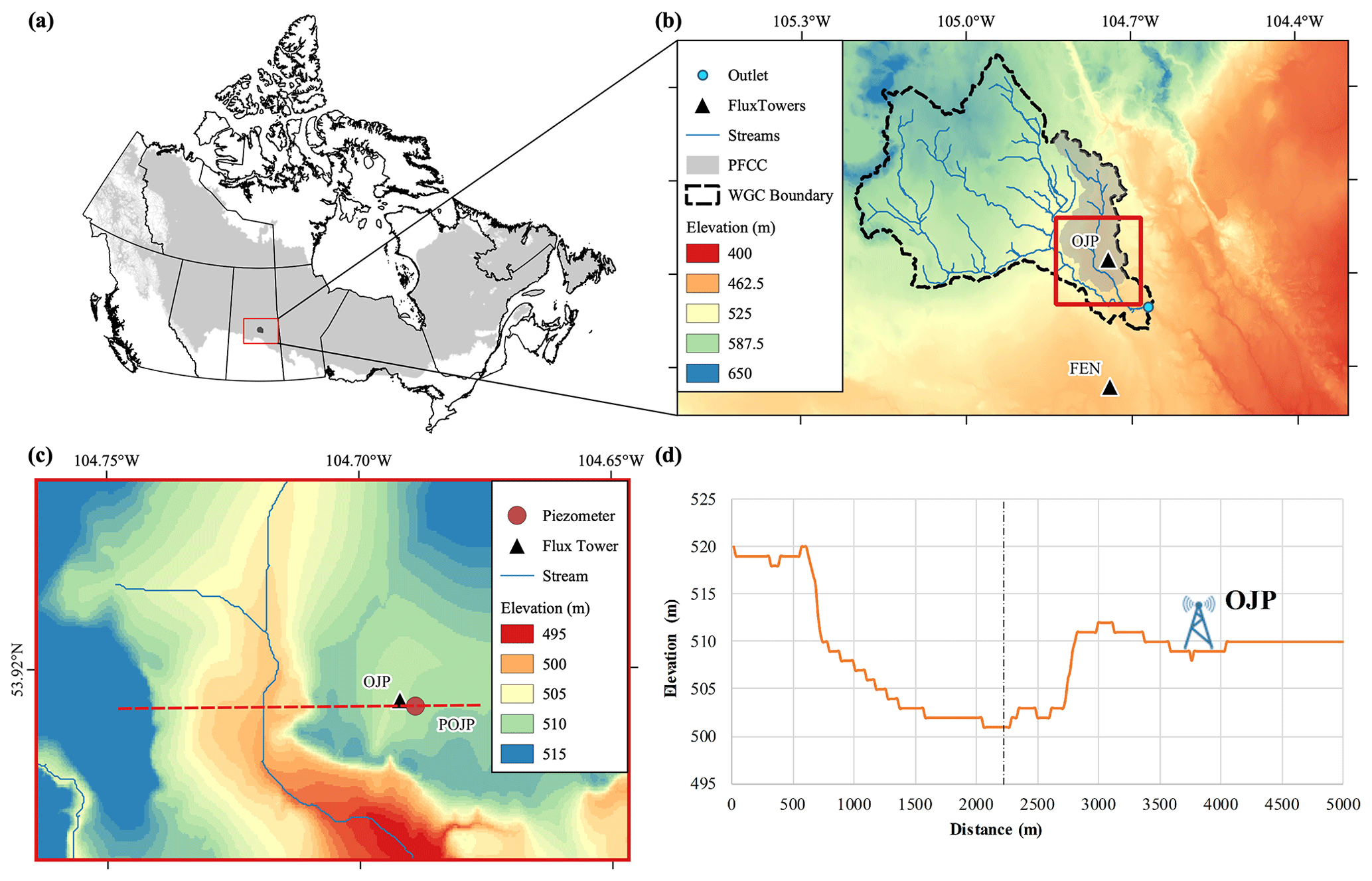
Figure 1Detailed view of the study area. Panel (a) presents Canada's boreal region (gray shading). Panel (b) provides a focused view of the White Gull Creek basin (WGCB) area and the two flux towers used in the study (Old Jack Pine, OJP, and Fen); the shaded gray area represents the Pine Fen Creek Catchment (PFCC) that includes the Pine Fen (PF). Panel (c) is a focused view of the OJP area, the piezometer at OJP (POJP), and the Pine Fen (PF). Panel (d) gives a cross-section of OJP and the PF (the dashed black line is assumed to be the line of symmetry).
The study area is located within the White Gull Creek basin (WGCB), located north of Prince Albert, Saskatchewan (Barr et al., 2012), as shown in Fig. 1. The study area and transect are set using the Canadian Digital Elevation Model (CDEM; Government of Canada, 2022).
The upland is the area around the Old Jack Pine (OJP) flux tower (53.92∘ N, 104.69∘ W; Fig. 1), which is part of the Boreal Ecosystem Research and Monitoring Sites (BERMS). The upland transect ends at the boundaries of the WGCB; the OJP site is located roughly in the middle of the transect (Fig. 1d) and is co-located with the piezometer (POJP; Fig. 1c) that is used to calibrate and validate the model performance. The transect length of 3450 m is divided into the upland hillslope (which is 3300 m in length) and the 150 m wide fen (which is half the total width of the fen). At the OJP site, the dominant land cover is Jack pine (Pinus banksiana Lamb.); the soil has a sandy texture, poor nutrition, and high drainage; and the water table is around 5 m below the ground (Barr et al., 2012). The meteorological data at OJP are available each 30 min for 23 years from 1997 to 2018. The GWT observations are available at the POJP location (Fig. 1) from 2003 to 2018.
The lowland part of our transect is a fen known as Pine Fen (PF) which is situated in Pine Fen Creek catchment (PFCC), a tributary of White Gull Creek (39.9 % of PFCC land cover is peatland) (Goodbrand et al., 2019). The PF site is a peatland mosaic surrounded by forests of Jack pine and black spruce. The average peat thickness is 0.65 m with a maximum depth of about 2 m. Unfortunately, we do not have direct meteorological observations from PF; therefore, as a proxy, we use observations from the BERMS fen flux tower site (FEN hereafter). FEN is located just outside the WGCB boundary, about 8 km south of the basin (53.78∘ N, 104.69∘ W; Fig. 1b). The FEN and PF sites are similar in terms of the peat soils, vegetation, and topography; therefore, FEN is considered a reasonable proxy for the vertical fluxes at PF. At FEN, forcing data are recorded with a 30 min resolution from 2003 to 2018, and the observed ET rates are from 2004 to 2010 and from 2013 to 2019 at 30 min intervals.
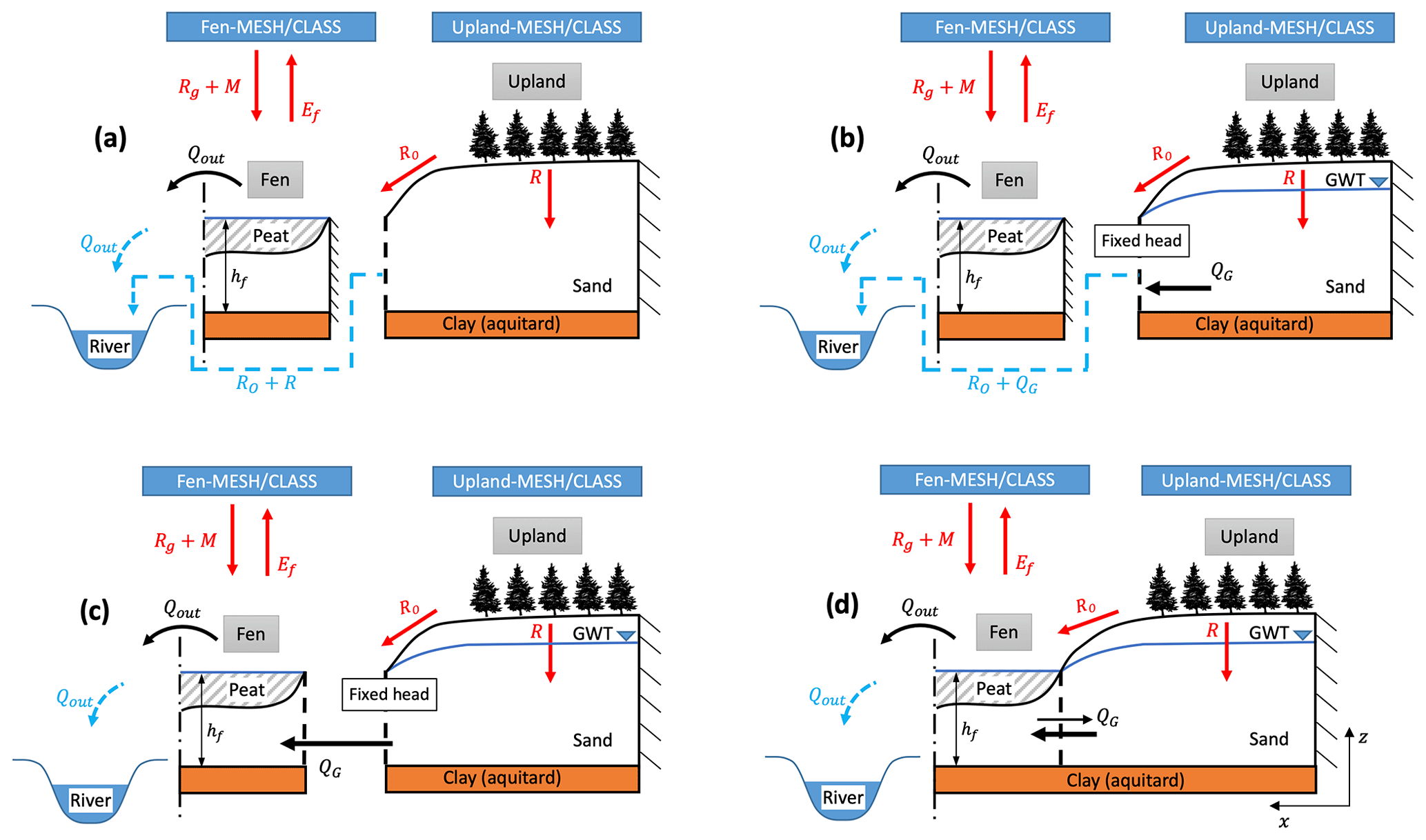
Figure 2Schematic of the different scenarios representing the connection between the upland, GW, and fen: (a) uncoupled upland–fen and no GW (V0), (b) uncoupled upland–GW–fen (V1), (c) chained model (V2), and (d) coupled model (V3). The vertical fluxes are rain on the ground (Rg), snowmelt (M), ET from the fen (Ef), and soil drainage as recharge into GW (R). The lateral fluxes are upland runoff (RO) and GW discharge (QG).
3.1 Conceptual background
Our study is based on a real field site, using real field observations, as described in the previous section. However, this site is not a perfectly constrained hillslope–fen system, i.e., a hillslope with 1D horizontal flow and a no-flow boundary condition at the interfluve. Therefore, we use an abstracted hypothetical hillslope configuration to simulate the vertical and lateral flows of water within the atmosphere–upland–GW–fen system. This configuration is physically realistic, allowing us to test the implications of different hillslope–fen coupling mechanisms in a controlled manner (Fig. 2).
Our model has three distinct components: (1) the upland soil water balance, which generates GW recharge and runoff; (2) a lateral GW flow model beneath the upland, which may discharge water into the fen; and (3) a simple fen water balance model, which receives inputs from rainfall, snowmelt, and runoff and lateral GW discharge (in some cases), and loses water to evaporation and discharge into a stream channel.
The model is driven by site observations of precipitation and other meteorological variables. A typical LSM is used to simulate ET fluxes in the upland and fen, GW recharge, runoff fluxes from the upland, and snowmelt into the fen. In this case, runoff fluxes are much smaller compared with the GW recharge. The water table and GW discharge are simulated by a simple 1D unconfined aquifer model. The water level at the fen and its discharge flux into an adjacent stream are simulated by a simple fen water balance model. The connections between the three models of the upland, GW, and fen are configured in four ways (as shown in Fig. 2), resulting in four different collective models:
- V0.
Uncoupled upland–fen model. The upland soil water balance and the fen are simulated as being independent of one another, and there is no GW model. Discharge from the upland in the form of surface runoff and soil drainage (baseflow) are combined with the fen discharge and routed into the river. This configuration is representative of many LSMs.
- V1.
Uncoupled upland–GW–fen model. Soil drainage from the upland recharges the unconfined aquifer. Surface runoff from the upland, GW discharge, and fen discharge are combined and routed into the river. The upland and the fen are again completely independent of one another. This configuration is representative of an LSM that has a GW store with a one-way vertical connection with the soil column, such as the Community Land Model (CLM) and the Variable Infiltration Capacity (VIC) model (Clark et al., 2015).
- V2.
Chained model. Soil drainage from the upland recharges the unconfined aquifer, and GW discharge contributes to storage into the fen. Discharge from the fen is routed into the river. GW is independent of the fen, but the fen depends on discharge from GW.
- V3.
Coupled model. Soil drainage from the upland recharges the unconfined aquifer. GW discharge into the fen is determined based on the head gradient between the GW and fen, and two-way water exchange is considered between the GW and fen. Surface runoff from the upland also goes into the fen. Discharge from the fen is routed into the river. The GW and fen are mutually dependent on one another.
3.2 Upland soil water balance model
The upland soil water balance is simulated using the MESH/CLASS land surface model (Canadian Land-surface scheme; Pietroniro et al., 2007; Wheater et al., 2022) with a point-scale set-up using the data from the OJP site, which is referred to as MESH_OJP hereafter. The land cover of the grid cell is represented by one canopy type – evergreen needle leaf – as most of the vegetation in the OJP area consists of Jack pine trees. MESH_OJP is forced using seven metrological components (precipitation, short-wave radiation, long-wave radiation, wind speed, specific humidity, temperature, and atmospheric pressure), which were collected from the OJP flux tower every 30 min from 1997 to 2018. The soil depth is assumed to equal 4.1 m and is divided into three layers (i.e., the default CLASS configuration). We are mainly interested in two outputs from the model: (1) soil drainage (R) is used as either baseflow to the river (V0) or recharge to the GW (V1, V2, and V3) and (2) surface runoff (RO) is used as SW input to the river (V0 and V1) or input to the fen (V2 and V3). The MESH/CLASS model uses an infiltration excess based on the Green–Ampt equation to calculate the soil infiltration, and the excess ponded water on the top of soil column is used to calculate the overland runoff.
3.3 Upland–GW model
The GW underneath the upland zone is represented as a 1D horizontal unconfined aquifer, bound by a no-flow boundary on the right (the GW divide) and the fen on the left (Fig. 2). The problem is governed by the 1D Boussinesq equation:
where Sy (unitless) is the specific yield, h (m) is the head in the aquifer (water table level), t (days) is time, K (m d−1) is the lateral hydraulic conductivity, and R (m d−1) is the recharge rate.
Equation 1 is solved numerically using a block-cantered finite-difference solution on a regularly spaced grid (, integrated in time using the method of lines with the SciPy ODE solver “odeint” (Virtanen et al., 2020), and the solution is coded up in Python. The lateral fluxes are calculated at cell boundaries using Darcy's law. The initial condition is assumed to be a uniform hydraulic head in the aquifer at the same water level as in the fen (hf). The right-hand boundary condition is considered to be a GW divide and, thus, a no-flow condition (. The flux on the left-hand boundary is determined using either a fixed head boundary (V1 and V2) or based on the head gradient between the GW and the fen (V3). The GW model is driven by the recharge fluxes (R), which are output from the upland soil water balance model and are assumed to be spatially uniform.
3.4 Fen water balance model
The fen is modelled as a simple lumped store, with the water balance equation:
where nf (unitless) is the porosity of the fen's material; wf (m) is the width of the fen; hf (m) is the water level of the fen; L (m) is the aquifer/hillslope length (in the x direction); , and RO (m d−1) are the rainfall, snowmelt, evaporation, and runoff from the upland, respectively; QG (m2 d−1) is the lateral GW inflow; and Qout (m2 d−1) is the outflow from the fen, assuming a unit area of 1 m in the y direction.
For Ef, Rg, and M, these fluxes are simulated by a point-scale MESH model using the data from the FEN site (hereafter referred to as MESH_FEN), which reasonably represent the conditions at the PF site. The forcing data (2003–2018) from the FEN flux tower are used to drive the MESH_FEN model. To simulate the peatland in the MESH/CLASS model, the land cover is assumed to be grass, while the soil type is set to organic soil with three soil layers of changing properties – fibric, hemic, and sapric (Letts et al., 2000). We manually calibrate the minimum stomatal resistance (rs,min = 100 s m−1) using local observations of the driving meteorological variables. We compared the simulated Ef with both the observed fluxes and with potential evaporation calculated using the Penman–Monteith equation, and we found that all three are consistent, showing that the evaporation from the FEN is unstressed (i.e., not water limited). The values of QG are either zero (V0 and V1) or equal to the GW discharge at the right-hand boundary (V2 and V3).
The values of Qout are generated when a spilling threshold, denoted as hspill, is exceeded. Qout is assumed to be a non-linear function of storage above hspill as given by the following:
Table 1Monte Carlo analysis parameter ranges for the uncoupled upland model.
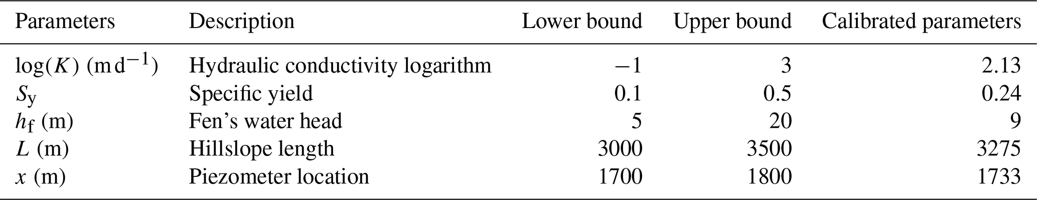
The value of hspill is assumed to equal the elevation of the fixed head boundary at the uncoupled GW model (Fig. 2b, c). The values of cspill and n (coefficient and exponent, respectively) are calibration parameters and are somewhat arbitrarily chosen within reasonable ranges. As there are no available outflow observations at the FEN site to allow for calibration, we adopt the recommended ranges provided by Razavi and Gupta (2019) for a fast reservoir with non-linear response (similar function/response to the fen storage). Razavi and Gupta (2019)'s values of k and α (coefficient and exponent, respectively) are utilized to define the cspill and n values (cspill=0.1 and n=1.5, respectively). While this approach lacks specific calibration for our site, it is deemed acceptable for achieving our study's objective, which is to compare different model configurations (V0, V1, V2, and V3) using the same parameters.
4.1 Calibration strategy
The performance of the different collective models is evaluated using the GWT observations at the POJP location by calculating the root-mean-square error (RMSE). For the upland water balance model, we use the same calibrated parameters as the study of Nazarbakhsh et al. (2020), who used the CLASS model to assess the controls on ET in a seasonally frozen forest. For the other parameters, Monte Carlo simulations with 15 000 realizations (randomly generated parameters from a uniform distribution bounded by the feasible parameter space in Table 1) are used to run the uncoupled upland–GW (V1) model. The behavioural runs are identified as the realizations with RMSE < 0.08 m (threshold is chosen arbitrarily based on expert judgement and calculated for the period from 2003 to 2009) and are used to perform the uncertainty analysis of the GWT simulation. The parameter set with lowest RMSE is considered the calibrated parameter set and is used to validate the model. This parameter set is also used to run all the other collective models throughout the study.
4.2 Effect of different upland properties
We develop two hypothetical numerical experiments to explore the conditions under which different levels of model complexity may be necessary. Experiment 1 focuses on hillslope geometry by considering five different values of the hillslope length (L, which is the length of the upland). L values of 100, 300, 500, 1000, 2000, and 3000 m are considered, and all other parameters are the same as in the original model set-up. This experiment uses the chained (V2) and the coupled (V3) versions of the model. Experiment 2 focuses on soil properties by comparing the original (sandy soil) set-up with a fine-grained soil representative of mineral soil that can typically be found in the prairie area. This is achieved using an alternative configuration of the MESH model in which the parameters are exchanged with values to represent a grass land cover and a fine-grained soil texture (clayey soil), resulting in different amounts of runoff, infiltration, and soil drainage. In the upland algorithm, the values of K and Sy are set to 1.35 m d−1 and 0.1, respectively, to characterize fine-grained soil. The simulated GWT and GW fluxes using the new MESH/CLASS run (representing fine-grained soil) are compared with the model results when using the original study set-up (upland algorithm forced with MESH_OJP).
We assess the performance of the model in the upland (Sect. 5.1) and fen (Sect. 5.2) independently. Next, in Sect. 5.3, we assess the sensitivity of the simulated outflow from the integrated upland–GW–fen system, which corresponds to the outflow at the grid-cell scale in LSMs (i.e., the bulk system outflow) to the different model configurations. Lastly, in Sect. 5.4, we describe the results of the two numerical experiments exploring the effect of changed upland properties and different wetland functionality.
5.1 Model performance in the upland
In the upland, the performance of the vertical land surface fluxes has been explored by Nazarbakhsh et al. (2020). We are able to assess the upland model's performance with respect to reproducing observations of the water table elevation. As explained earlier, there is no GW in V0 of the model. In the uncoupled (V1) and chained (V2) models, the GW simulations are identical. In the coupled model (V3), the water table simulations may, in principle, differ from those in V1 and V2. Therefore, we compare V1 and V3 separately here.
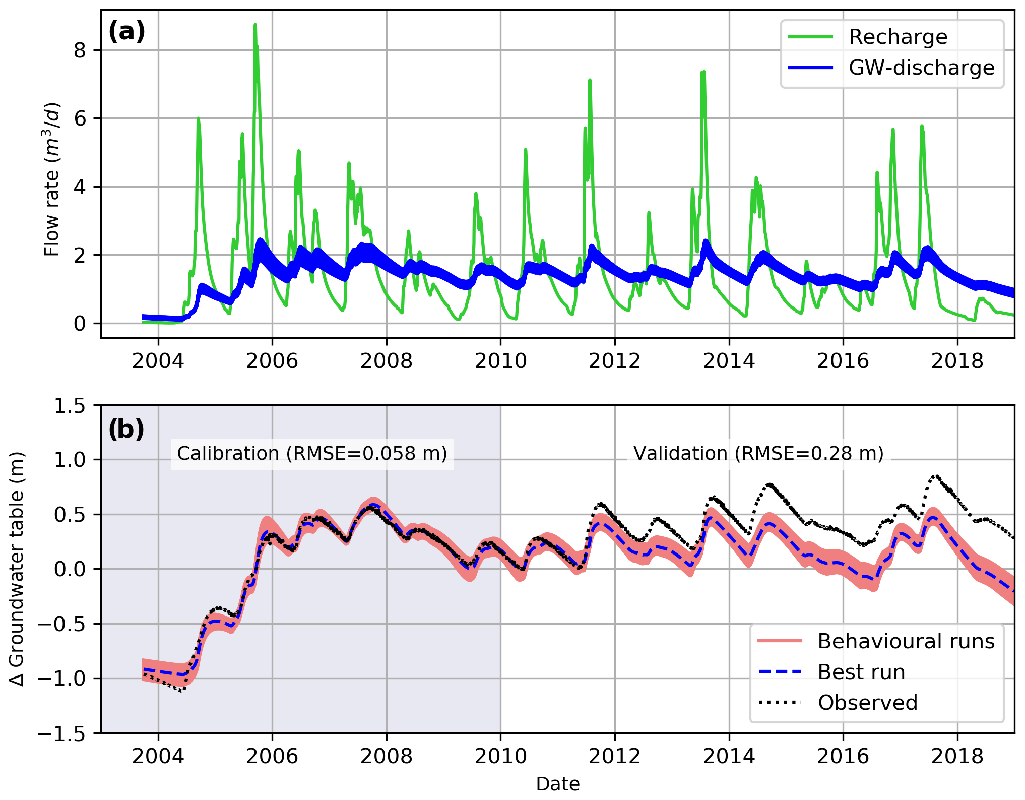
Figure 3Panel (a) shows the upland recharge rates into the GW aquifer that are generated using the MESH_OJP model and used to drive the upland component. Panel (b) presents a comparison between the simulated (V1) and observed changes in the GWT at the OJP site. The uncertainty results (GW discharge and GWT) are obtained from the behavioural realizations using Monte Carlo analysis.
5.1.1 Uncoupled model calibration and validation
The upland component in the uncoupled model is driven by the recharge values that are generated using the MESH_OJP model (Fig. 3a). Figure 3b shows a comparison between the simulated and observed GWT at the OJP site using the uncoupled upland model. The behavioural runs (69 runs with an RMSE < 0.08 m) from Monte Carlo analysis are used to generate the uncertainty bounds in the simulation of both GW discharge and GWT (Fig. 3). It can be seen from Fig. 3a that the recharge and the simulated GW discharge responded to each other consistently. Also, the changes in the GWT corresponded to both the recharge and the GW discharge peaks.
For the uncoupled upland model, the best RMSE value is equal to 0.058 m for calibration and 0.28 m for validation. The uncoupled upland model can simulate the GWT in the calibration period with a narrow uncertainty bound. In the validation period, the simulated GWT matched the observations until the spring of 2011, when a discrepancy is noticed, and the GWT is underestimated thereafter. The GWT underestimation is caused by low recharge rates from 2011 to the end of the simulation, which might be caused by either undercatch in the observed precipitation or problems with the MESH/CLASS model with respect to simulating the recharge rates in this period. The MESH/CLASS model problem could be because of the overestimation of ET rates at the upland site, which means that the MESH/CLASS model might need recalibration to a longer period of data. The reason for the overestimation of ET rates at OJP could be the missing representation of the wetland and GW system in the MESH model (see Figs. S1 and S2 in the Supplement). We should note that, although the model showed underestimation of the GWT magnitude (from 2011 to 2018), it captured the same pattern during the same period. Based on its performance, we believe that our model acceptably serves its purpose, as the main aim of this study is to perform numerical experiments to help us understand the upland–GW–fen system dynamics.
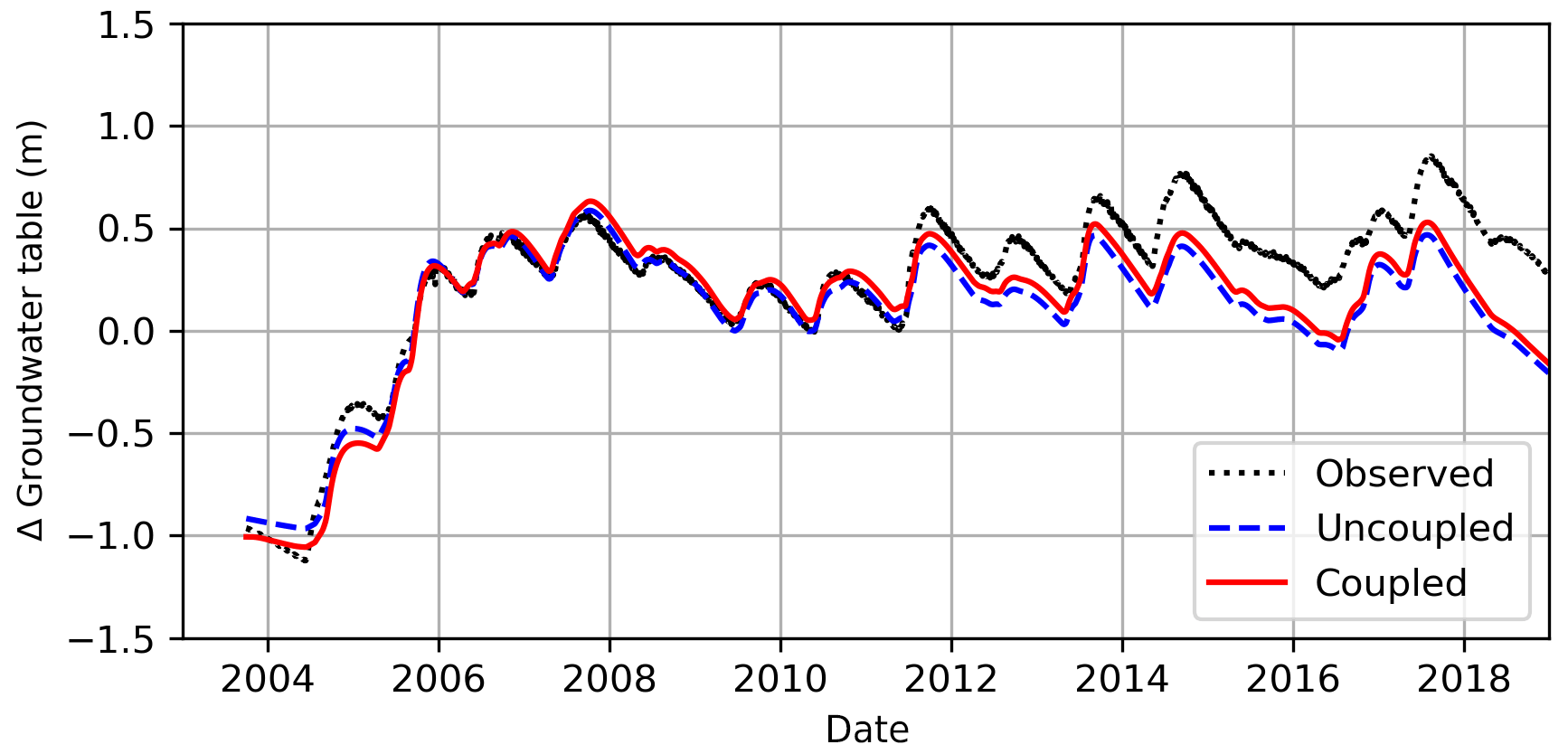
Figure 4Comparison between the simulated GWT using both the uncoupled and coupled models with the observations.
5.1.2 Upland – uncoupled vs. coupled
Figure 4 shows a comparison between the simulated GWT using the uncoupled/chained (V1/V2) and coupled (V3) model versions and using the observations (note that the upland is still uncoupled, as in V1, in the V2 model configuration). The overall performance of the coupled version showed only a slight improvement (RMSE = 0.18 m) over the uncoupled version (RMSE = 0.22 m). A comparison between the simulated uncoupled and coupled systems shows that, in the period of record, considering the effect of the fen system does not affect the simulated GWT underneath the upland in the case of OJP and PF. However, the impact of this coupling might become more profound for other sites with different settings or the same site under different climate conditions.
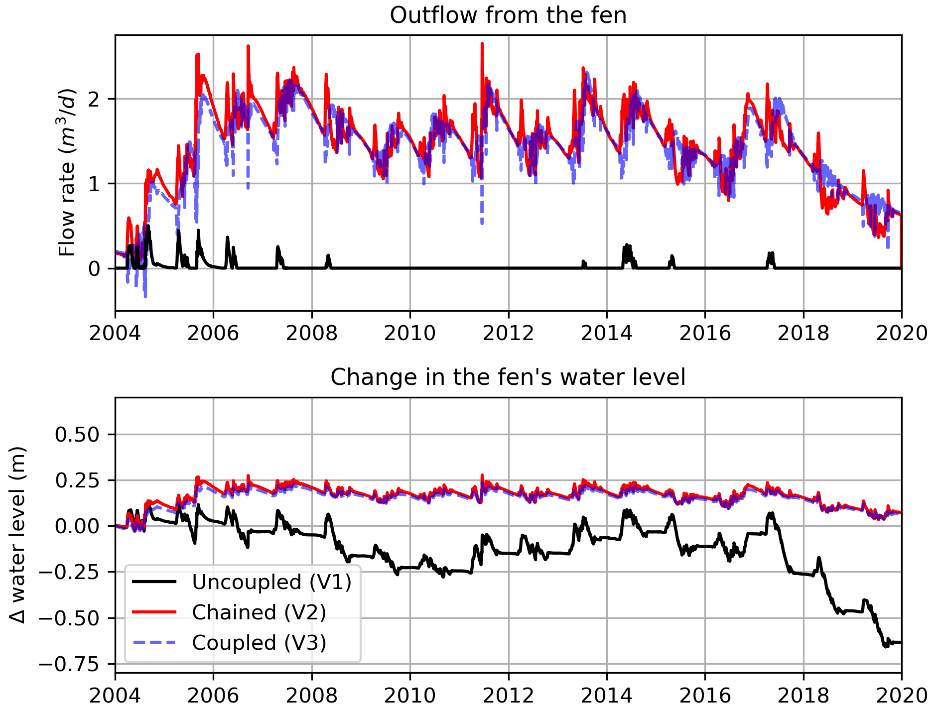
Figure 5Comparison between the fen's output (fen outflow and change in the fen water level) for the three modelling scenarios: uncoupled (V1), chained (V2), and coupled (V3).
5.2 Model performance in the fen
For the fen, we are not able to directly test our model performance due to a lack of data; instead, we explore the sensitivity of the fluxes to the change in the modelling configuration (interaction between the upland and fen). The fen's outflow and changes in water level are compared for the three model versions (V1, V2, and V3) in Fig. 5. In the uncoupled (V1) model, when there is no GW inflow to the fen, the estimated outflow and water level changes are unrealistic, as the outflow is almost zero and the water level kept decreasing from one year to another. On the other hand, the chained (V2) and coupled (V3) models had a reasonable simulation of the outflow and water level changes in the fen, although with differences from each other, particularly in terms of the flow rate. The overall trends in the flow rates of V2 and V3 look similar, but the higher-frequency features (e.g., daily flows) show different dynamics from time to time. The flow rates of V3 are affected by the two-way water exchange between the upland and fen, which are based on the variable fen water level, unlike the concept of a constant fen water level that is used in V2. This is apparent in 2004, wherein the V3 model generated negative flow rates (i.e., water flows from the fen into the upland). This comparison shows that the GW inflow from the upland into the fen cannot be ignored when simulating the fen; however, the chained modelling approach might be deemed adequate to capture the fen system dynamics. A coupled configuration is needed to study the short-term impacts and changes in the fen outflow.
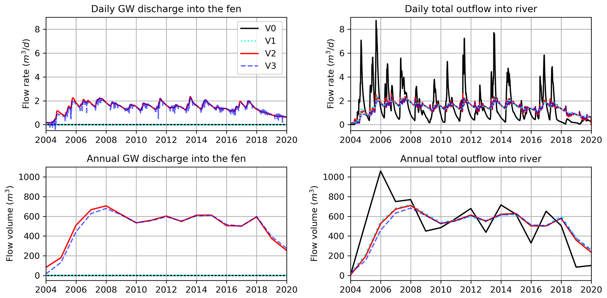
Figure 6Comparison between GW discharge into the fen and total outflow from the grid cell into the river at daily and annual scales for the V0–V3 modelling scenarios (Fig. 2).
5.3 Outflow of the integrated upland–fen system (grid-cell scale)
In this section, we investigated the total outflow from the integrated upland–GW–fen system as a whole unit under different modelling configurations, which are the possible approaches to represent such system in LSMs, to simulate the amount of the total flow that discharges into the river network (streamflow; see the dashed blue arrows in Fig. 2). In LSMs, a grid cell can contain multiple components, such as upland and fen. In this case, the total outflow of the grid cell is the combined outflow from both the upland and fen components after considering the interaction between them based on the used modelling configuration. This is done to assess the optimal level of model complexity that can simulate the streamflow adequately.
In the chained (V2) and coupled (V3) models, the simulated GW discharge into the fen from both models is almost the same at a daily and annual scale (Fig. 6). Also, the total outflow from the grid cell into river showed no significant difference in the two cases. In the case of the uncoupled upland–GW–fen model (V1), there is no GW discharge into the fen, but the daily and annual total outflow into the river is similar to that of V2 and V3. Therefore, at the grid-cell scale, the interaction between the upland and the fen had no effect on the total outflow from the grid cell nor discharge into the river for our model configuration.
In the case of V0, GW storage is not accounted for, and all of the soil drainage (recharge) is considered to be baseflow, which is discharged directly into the river network (the case in most of the current LSMs). Therefore, the simulated outflow (of V0) into the river is significantly different (with overall greater magnitudes) compared with the other three versions that account for GW storage (Fig. 6). This means that consideration of the GW dynamics underneath the upland is essential for a reasonable simulation of the total streamflow into the river network.
5.4 The effect of different upland properties on upland–fen interactions
Here, we run two additional numerical experiments to explore the optimal level of modelling complexity for different upland site properties. The experiments are hypothetical (no observations) and represent other possible sites' conditions.
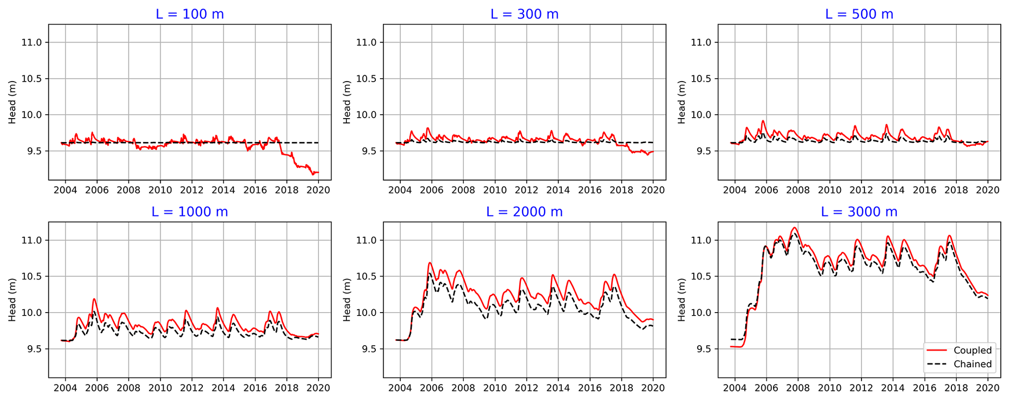
Figure 7Simulated upland GWT for both the chained and coupled model versions using different hillslope length (L) values.
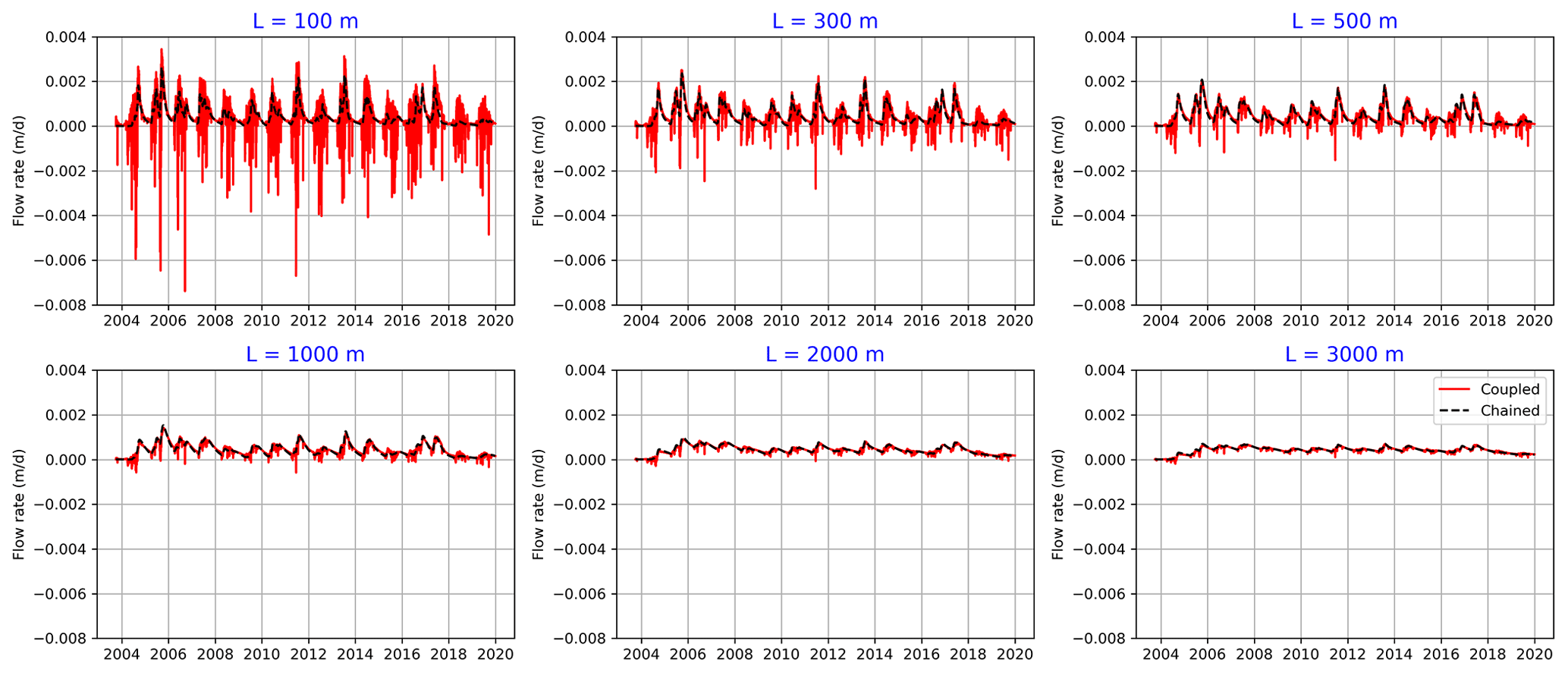
Figure 8Simulated upland GW fluxes for both the chained and coupled model versions using different hillslope length (L) values.
5.4.1 Experiment 1: different hillslope lengths
Figure 7 shows the simulated upland GWT using different upland hillslope lengths (width of the fen is constant) and compares the results in the case of chained (V2) and coupled (V3) upland configurations. In the case of horizontally large aquifers (L > 1000 m), as in our original study set-up, there is no significant difference in the simulated GWT and GW flux when using the two model configurations. In contrast, for small hillslopes (lengths between 100 and 500 m), the chained model is not able to reasonably capture the fluctuations in the upland GWT (GWT is almost constant), due to a fixed head boundary condition on the upland side. Also, the difference can be seen when comparing the simulated GW fluxes in the two model configurations (Fig. 8). For small hillslopes, the coupled model can capture the water amounts that move from the fen into the upland (negative flux values), which are considerable amounts that are frequently present throughout the year.
For large hillslopes, the GW size (extent) is significantly greater than the fen size (140 m); therefore, large amounts of water move from the upland area into the fen. As a result, the upland area controls the dynamics of the whole system. In such cases, the upland can be simulated independently with no consideration of interaction with the fen. In the case of small hillslopes, however, the fen is the dominant contributor to the system, as the water moves continually in both directions. In such cases, the coupling between the upland and fen is essential.
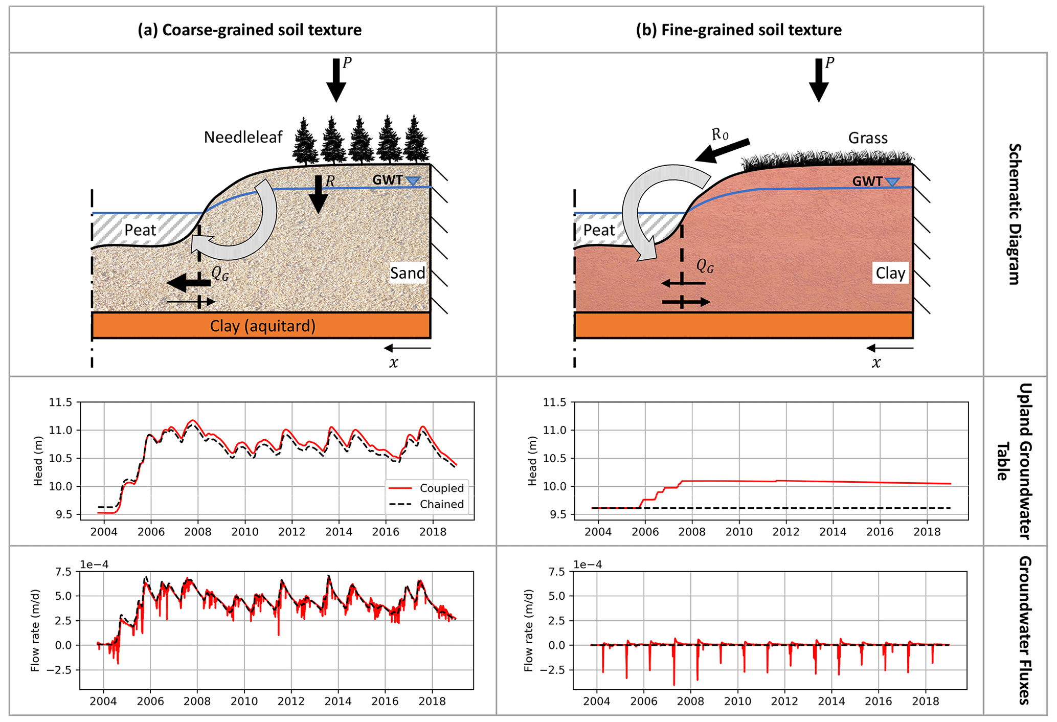
Figure 9Comparison between two different upland site conditions and the simulated upland GWT in each case: (a) OJP with a coarse-grained soil texture and evergreen needleleaf canopy and (b) St. Denis with a fine-grained soil texture and grass land cover.
5.4.2 Experiment 2: different upland soil properties
Figure 9 illustrates a comparison between two upland cases: (1) coarse-grained soil (high permeability) and forest land cover (dense vegetation) with a long hillslope length, which is our original study set-up (Fig. 9a), and (2) fine-grained soil (low permeability) and grass land cover (Fig. 9b). In MESH_OJP, changing the vegetation type impacts ET rates from the upland and RO, whereas altering the soil properties affects the infiltrated water and R rates. In this experiment, the first case represents the original model configuration at OJP, whereas the second case is designed to maximize surface runoff from the upland into the wetland. This provides a contrasting scenario with a different wetland type (other than a fen), in contrast to the GW-dependent wetland case. The parameters used to configure the MESH model for the second case are based on a model configuration presented in Ireson and Sanchez-Rodriguez (2021) and are similar to the parameters and properties of the St. Denis site.
In the case of coarse-grained soil (Fig. 9a), the main contribution to the upland GW system is high recharge rates because of the high infiltrability of the soil (coarse-grained/sandy) and the relatively small amounts of surface runoff to the fen. Thus, in this case, the dominant component of the upland–fen system is the GW fluxes from the upland into the fen (through subsurface water movement). Water arrives as precipitation on the upland, infiltrates into the soil and recharges the aquifer, and finally moves laterally in the aquifer to discharge into the fen. To represent these system dynamics, the chained (V2) modelling approach for the upland system seems adequate to simulate the GW system (GWT and GW discharge) of the upland (this might not be applicable to relatively small hillslopes, as demonstrated in Experiment 1 in Sect. 5.4.1), as the difference between the results when using the chained (V2) and coupled (V3) models is relatively small (Fig. 9a). However, the coupled (V3) model can simulate the dynamics of the daily GW flows due to the frequent change in the fen water level. Accordingly, the flow direction is reversed to be from the fen into the upland (negative flow values) from 2004 to 2005 (Fig. 9a).
The system dynamics are different when the soil has a fine-grained texture and the vegetation has a low density (Fig. 9b). In this case, large amounts of surface runoff move directly from the hillslope into the wetland, whereas very limited amounts of water may infiltrate into the upland aquifer. Figure 9b shows that the chained model is not able to simulate any of the GW dynamics underneath the upland, whereas the coupled model captured the system dynamics (GW fluxes in Fig. 9b). In this case, the wetland is mainly fed by the surface runoff fluxes, and the water moves laterally into the upland (especially during snowmelt season). Hence, the main flow path is from the wetland into the upland GW. Therefore, the upland GW dynamics are dominated by the subsurface water fluxes coming from the neighbouring wetlands. It is obvious that considering only the chained approach (one-way exchange between the upland and wetland) in the case of fine-grained upland soil cannot reasonably capture the real dynamics of the system. However, the full coupling between the upland and the wetland (two-way water exchange) allows the model to represent the actual dynamics of the upland aquifer underneath fine-grained soil layers.
The insights gained from applying alternative model configurations to the upland–fen system in this study are as follows:
-
We were able to reasonably simulate the GW dynamics underneath the upland using the 1D Boussinesq equation. There are no significant differences between the coupled and uncoupled modelling approaches with respect to simulating the upland water table elevation, as the dominant flow direction is from the upland to the fen.
-
To accurately simulate the water level in the fen, it is important not to ignore the GW input from the upland. However, there is no significant difference between the chained (one-way interaction) and coupled (two-way interaction) approaches in terms of the simulated fen water level and outflow.
-
Including upland–fen interactions had no significant impact on the discharge into the river network. However, the inclusion of GW storage had a major impact on the timing and magnitude of river discharge.
We found that a coupled fen–upland modelling approach becomes essential when the size of the fen is large relative to the upland area. This is due to substantial bidirectional water exchanges between the fen and the upland GW at various times of the year. The coupled modelling approach is also more likely to be necessary when simulating uplands with fine-grained soils. In this case, the wetland receives more surface runoff and less GW input, resulting in a significant loss of water to the GW system.
In general, if the main objective of the model is to simulate streamflow, the coupling (two-way interaction) between the upland and fen (or GW-dependent wetland types) can likely be ignored. However, GW dynamics must be represented in LSMs, as they significantly affect the total outflow (streamflow) from the entire system. Conversely, if the simulation of the storage and fluxes within fen/wetlands are of interest, the chained modelling approach represents the least complex level necessary to account for the contributions of the surrounding upland and GW systems.
This study provides insights into the necessary model complexity for simulating an upland–GW–fen system within LSMs. The outcomes of this study can aid in improving process representation in LSMs and guiding current and future hydrological modelling practices in fen-dominated areas. However, other types of wetlands need more investigation using data/observations including different site conditions. This can result in more accurate simulation of the water cycle in those regions, contributing to enhanced water resource management and allocation as well as improving LSMs' ability to predict the effects of future climate change on wetlands.
We used WISKI (the Water Information Systems by KISTERS) data. These data are publicly available from https://wiki.usask.ca/display/GWFDM/WISKI (last access: October 2023) and were downloaded using the Python WISKI tool (https://github.com/incsanchezro/WISKI_Tools_GWF, Ireson, 2023). The meteorological data used in this work were from the Old Jack Pine (OJP) and Fen flux towers, and the upland GW observations were from OJP. The models developed and used in this paper are available from Zenodo: https://doi.org/10.5281/zenodo.8277901 (Elrashidy et al., 2023).
The supplement related to this article is available online at: https://doi.org/10.5194/hess-27-4595-2023-supplement.
MTE: conceptualization, methodology, model development, and writing; AMI: conceptualization, methodology, model development, and writing (review and editing); and SR: conceptualization, methodology, and writing (review and editing).
The contact author has declared that none of the authors has any competing interests.
Publisher's note: Copernicus Publications remains neutral with regard to jurisdictional claims made in the text, published maps, institutional affiliations, or any other geographical representation in this paper. While Copernicus Publications makes every effort to include appropriate place names, the final responsibility lies with the authors.
The authors would like to thank the Global Water Futures (GWF) and the Integrated Modelling Program for Canada (IMPC) for funding this research.
This research has been supported by the Global Water Futures .
This paper was edited by Christa Kelleher and reviewed by two anonymous referees.
Barr, A. G., van der Kamp, G., Black, T. A., McCaughey, J. H., and Nesic, Z.: Energy balance closure at the BERMS flux towers in relation to the water balance of the White Gull Creek watershed 1999–2009, Agr. Forest Meteorol., 153, 3–13, https://doi.org/10.1016/j.agrformet.2011.05.017, 2012.
Blyth, E. M., Arora, V. K., Clark, D. B., Dadson, S. J., De Kauwe, M. G., Lawrence, D. M., Melton, J. R., Pongratz, J., Turton, R. H., Yoshimura, K., and Yuan, H.: Advances in Land Surface Modelling, Curr. Clim. Change Rep., 7, 45–71, https://doi.org/10.1007/s40641-021-00171-5, 2021.
Canada Committee on Ecological (Biophysical) Land Classification (Ed.): Wetlands of Canada, Sustainable Development Branch, Canadian Wildlife Service, Conservation and Protection, Environment Canada, Ottawa, 452 pp., 1988.
Clark, M. P., Fan, Y., Lawrence, D. M., Adam, J. C., Bolster, D., Gochis, D. J., Hooper, R. P., Kumar, M., Leung, L. R., Mackay, D. S., Maxwell, R. M., Shen, C., Swenson, S. C., and Zeng, X.: Improving the representation of hydrologic processes in Earth System Models: REPRESENTING HYDROLOGIC PROCESSES IN EARTH SYSTEM MODELS, Water Resour. Res., 51, 5929–5956, https://doi.org/10.1002/2015WR017096, 2015.
Dai, Y., Zeng, X., Dickinson, R. E., Baker, I., Bonan, G. B., Bosilovich, M. G., Denning, A. S., Dirmeyer, P. A., Houser, P. R., Niu, G., Oleson, K. W., Schlosser, C. A., and Yang, Z.-L.: The Common Land Model, B. Am. Meteorol. Soc., 84, 1013–1024, https://doi.org/10.1175/BAMS-84-8-1013, 2003.
Davison, B., Pietroniro, A., Fortin, V., Leconte, R., Mamo, M., and Yau, M. K.: What is Missing from the Prescription of Hydrology for Land Surface Schemes?, J. Hydrometeor., 17, 2013–2039, https://doi.org/10.1175/JHM-D-15-0172.1, 2016.
de Graaf, I. E. M., van Beek, R. L. P. H., Gleeson, T., Moosdorf, N., Schmitz, O., Sutanudjaja, E. H., and Bierkens, M. F. P.: A global-scale two-layer transient groundwater model: Development and application to groundwater depletion, Adv. Water Resour., 102, 53–67, https://doi.org/10.1016/j.advwatres.2017.01.011, 2017.
Elrashidy, M. T., Ireson, A. M., and Razavi, S.: On the optimal level of complexity for the representation of groundwater-dependent wetland systems in land surface models, in: Hydrology and Earth System Sciences, Zenodo [data set], https://doi.org/10.5281/zenodo.8277901, 2023.
Fan, Y., Li, H., and Miguez-Macho, G.: Global Patterns of Groundwater Table Depth, Science, 339, 940–943, https://doi.org/10.1126/science.1229881, 2013.
Fan, Y., Clark, M., Lawrence, D. M., Swenson, S., Band, L. E., Brantley, S. L., Brooks, P. D., Dietrich, W. E., Flores, A., Grant, G., Kirchner, J. W., Mackay, D. S., McDonnell, J. J., Milly, P. C. D., Sullivan, P. L., Tague, C., Ajami, H., Chaney, N., Hartmann, A., Hazenberg, P., McNamara, J., Pelletier, J., Perket, J., Rouholahnejad-Freund, E., Wagener, T., Zeng, X., Beighley, E., Buzan, J., Huang, M., Livneh, B., Mohanty, B. P., Nijssen, B., Safeeq, M., Shen, C., Verseveld, W., Volk, J., and Yamazaki, D.: Hillslope Hydrology in Global Change Research and Earth System Modeling, Water Resour. Res., 55, 1737–1772, https://doi.org/10.1029/2018WR023903, 2019.
Gingras, B., Slattery, S., Smith, K., and Darveau, M.: Boreal Wetlands of Canada and the United States of America, in: The Wetland Book: II: Distribution, Description, and Conservation, edited by: Finlayson, C. M., Milton, G. R., Prentice, R. C., and Davidson, N. C., Springer Netherlands, Dordrecht, 521–542, https://doi.org/10.1007/978-94-007-4001-3_9, 2018.
Goodbrand, A., Westbrook, C. J., and van der Kamp, G.: Hydrological functions of a peatland in a Boreal Plains catchment, Hydrol. Process., 33, 562–574, https://doi.org/10.1002/hyp.13343, 2019.
Goodbrand, A. R.: Influence of lakes and peatlands on groundwater contribution to boreal streamflow, MSc Thesis, University of Saskatchewan, 2013.
Ireson, A. and Sanchez-Rodriguez, I.: WISKI Tools GWF, https://github.com/incsanchezro/WISKI_Tools_GWF (last access: October 2023), 2021.
Ireson, A. M., Sanchez-Rodriguez, I., Basnet, S., Brauner, H., Bobenic, T., Brannen, R., Elrashidy, M., Braaten, M., Amankwah, S. K., and Barr, A.: Using observed soil moisture to constrain the uncertainty of simulated hydrological fluxes, Hydrol. Process., 36, e14465, https://doi.org/10.1002/hyp.14465, 2022.
Government of Canada: Canadian Digital Elevation Model, 1945–2011 – Open Government Portal: https://open.canada.ca/data/en/dataset/7f245e4d-76c2-4caa-951a-45d1d2051333, last access: 14 December 2022.
Kollet, S. J. and Maxwell, R. M.: Capturing the influence of groundwater dynamics on land surface processes using an integrated, distributed watershed model, Water Resour. Res., 44, W02402, https://doi.org/10.1029/2007WR006004, 2008.
Letts, M. G., Roulet, N. T., Comer, N. T., Skarupa, M. R., and Verseghy, D. L.: Parametrization of peatland hydraulic properties for the Canadian land surface scheme, Atmos. Ocean, 38, 141–160, https://doi.org/10.1080/07055900.2000.9649643, 2000.
Manabe, S.: CLIMATE AND THE OCEAN CIRCULATION: I. THE ATMOSPHERIC CIRCULATION AND THE HYDROLOGY OF THE EARTH'S SURFACE, Mon. Weather Rev., 97, 739–774, https://doi.org/10.1175/1520-0493(1969)097<0739:CATOC>2.3.CO;2, 1969.
Maxwell, R. M. and Miller, N. L.: Development of a Coupled Land Surface and Groundwater Model, J. Hydrometeor., 6, 233–247, https://doi.org/10.1175/JHM422.1, 2005.
Maxwell, R. M., Condon, L. E., and Kollet, S. J.: A high-resolution simulation of groundwater and surface water over most of the continental US with the integrated hydrologic model ParFlow v3, Geosci. Model Dev., 8, 923–937, https://doi.org/10.5194/gmd-8-923-2015, 2015.
Mitsch, W. J., Bernal, B., Nahlik, A. M., Mander, Ü., Zhang, L., Anderson, C. J., Jørgensen, S. E., and Brix, H.: Wetlands, carbon, and climate change, Landscape Ecol., 28, 583–597, https://doi.org/10.1007/s10980-012-9758-8, 2013.
Nazarbakhsh, M., Ireson, A. M., and Barr, A. G.: Controls on evapotranspiration from jack pine forests in the Boreal Plains Ecozone, Hydrol. Process., 34, 927–940, https://doi.org/10.1002/hyp.13674, 2020.
Ogden, F. L.: Geohydrology: Hydrological Modeling, in: Encyclopedia of Geology (Second Edition), edited by: Alderton, D. and Elias, S. A., Academic Press, Oxford, 457–476, https://doi.org/10.1016/B978-0-08-102908-4.00115-6, 2021.
Pietroniro, A., Fortin, V., Kouwen, N., Neal, C., Turcotte, R., Davison, B., Verseghy, D., Soulis, E. D., Caldwell, R., Evora, N., and Pellerin, P.: Development of the MESH modelling system for hydrological ensemble forecasting of the Laurentian Great Lakes at the regional scale, Hydrol. Earth Syst. Sci., 11, 1279–1294, https://doi.org/10.5194/hess-11-1279-2007, 2007.
Razavi, S. and Gupta, H. V.: A multi-method Generalized Global Sensitivity Matrix approach to accounting for the dynamical nature of earth and environmental systems models, Environ. Modell. Softw, 114, 1–11, https://doi.org/10.1016/j.envsoft.2018.12.002, 2019.
Razavi, S., Hannah, D. M., Elshorbagy, A., Kumar, S., Marshall, L., Solomatine, D. P., Dezfuli, A., Sadegh, M., and Famiglietti, J.: Coevolution of machine learning and process-based modelling to revolutionize Earth and environmental sciences: A perspective, Hydrol. Process., 36, e14596, https://doi.org/10.1002/hyp.14596, 2022.
Rivera, A. (Ed.): Canada's groundwater resources, Fitzhenry & Whiteside, Markham, ON, 803 pp., ISBN 1554552923, 9781554552924, 2014.
Scheidegger, J. M., Jackson, C. R., Muddu, S., Tomer, S. K., and Filgueira, R.: Integration of 2D Lateral Groundwater Flow into the Variable Infiltration Capacity (VIC) Model and Effects on Simulated Fluxes for Different Grid Resolutions and Aquifer Diffusivities, Water, 13, 663, https://doi.org/10.3390/w13050663, 2021.
Virtanen, P., Gommers, R., Oliphant, T. E., Haberland, M., Reddy, T., Cournapeau, D., Burovski, E., Peterson, P., Weckesser, W., Bright, J., van der Walt, S. J., Brett, M., Wilson, J., Millman, K. J., Mayorov, N., Nelson, A. R. J., Jones, E., Kern, R., Larson, E., Carey, C. J., Polat, İ., Feng, Y., Moore, E. W., VanderPlas, J., Laxalde, D., Perktold, J., Cimrman, R., Henriksen, I., Quintero, E. A., Harris, C. R., Archibald, A. M., Ribeiro, A. H., Pedregosa, F, van Mulbregt, P.; SciPy 1.0 Contributors: SciPy 1.0: fundamental algorithms for scientific computing in Python, Nat Methods, 17, 261–272, https://doi.org/10.1038/s41592-019-0686-2, 2020.
Wheater, H. S., Pomeroy, J. W., Pietroniro, A., Davison, B., Elshamy, M., Yassin, F., Rokaya, P., Fayad, A., Tesemma, Z., Princz, D., Loukili, Y., DeBeer, C. M., Ireson, A. M., Razavi, S., Lindenschmidt, K.-E., Elshorbagy, A., MacDonald, M., Abdelhamed, M., Haghnegahdar, A., and Bahrami, A.: Advances in modelling large river basins in cold regions with Modélisation Environmentale Communautaire—Surface and Hydrology (MESH), the Canadian hydrological land surface scheme, Hydrol. Process., 36, e14557, https://doi.org/10.1002/hyp.14557, 2022.
Yalew, S. G., Pilz, T., Schweitzer, C., Liersch, S., van der Kwast, J., van Griensven, A., Mul, M. L., Dickens, C., and van der Zaag, P.: Coupling land-use change and hydrologic models for quantification of catchment ecosystem services, Environ. Modell. Softw., 109, 315–328, https://doi.org/10.1016/j.envsoft.2018.08.029, 2018.
Zampieri, M., Serpetzoglou, E., Anagnostou, E. N., Nikolopoulos, E. I., and Papadopoulos, A.: Improving the representation of river–groundwater interactions in land surface modeling at the regional scale: Observational evidence and parameterization applied in the Community Land Model, J. Hydrol., 420–421, 72–86, https://doi.org/10.1016/j.jhydrol.2011.11.041, 2012.
Zeng, Y., Xie, Z., Liu, S., Xie, J., Jia, B., Qin, P., and Gao, J.: Global Land Surface Modeling Including Lateral Groundwater Flow, J. Adv. Model. Earth Sy., 10, 1882–1900, https://doi.org/10.1029/2018MS001304, 2018.