A pulse-decay method for low (matrix) permeability analyses of granular rock media

Nanodarcy level permeability measurements of porous media, such as nano-porous mudrocks, are frequently conducted with gas invasion methods into granular-sized samples with short diffusion lengths and thereby reduced experimental duration; however, these methods lack rigorous solutions and standardized experimental procedures. For the first time, we resolve this by providing an integrated technique (termed gas permeability technique, GPT) with coupled theoretical development, experimental procedures, and data interpretation workflow. Three exact mathematical solutions for transient and slightly compressible spherical flow, along with their asymptotic solutions, are developed for early- and late-time responses. Critically, one late-time solution is for an ultra-small gas-invadable volume, important for a wide range of practical usages. Developed to be applicable to different sample characteristics (permeability, porosity, and mass) in relation to the storage capacity of experimental systems, these three solutions are evaluated from essential considerations of error difference between exact and approximate solutions, optimal experimental conditions, and experimental demonstration of mudrocks and molecular-sieve samples. Moreover, a practical workflow of solution selection and data reduction to determine permeability is presented by considering samples with different permeability and porosity under various granular sizes. Overall, this work establishes a rigorous, theory-based, rapid, and versatile gas permeability measurement technique for tight media at sub-nanodarcy levels.

1 Introduction

Shales, crystalline, and salt rocks with low permeabilities (e.g., <10⁻¹⁷ m² or approximately 10 microdarcy, µd) are critical components in numerous subsurface studies. Notable examples are the remediation of contaminated sites (Neuzil, 1986; Yang et al., 2015), long-term performance of high-level nuclear waste repositories (Kim et al., 2011; Neuzil, 2013), enhanced geothermal systems (Huenges, 2016; Zhang et al., 2021), efficient development of unconventional oil and gas resources (Hu et al., 2015; Javadpour, 2009), long-term sealing for carbon utilization and storage (Fakher et al., 2020; Khosrokhavar, 2016), and high-volume and effective gas (hydrogen) storage (Liu et al., 2015; Tarkowski, 2019). For fractured rocks, the accurate characterization of rock matrix and its permeability is also critical for evaluating the effectiveness of low-permeability media, particularly when transport is dominated by slow processes like diffusion (Ghanbarian et al., 2016; Hu et al., 2012).

Standard permeability test procedures in both steady-state and pulse-decay methods use consolidated centimeter-sized core-plug samples, which may contain fractures and show dual- or triple-porosity characteristics (Abdassah and Ershaghi, 1986; Bibby, 1981). The overall permeability may therefore be controlled by a few bedding-oriented or cross-cutting fractures, even if experiments are conducted at reservoir pressures (Bock et al., 2010; Gensterblum et al., 2015; Gutierrez et al., 2000; Luffel et al., 1993). Fractures might be naturally or artificially induced (e.g., created during sample processing), which makes a comparison of permeability results among different samples difficult (Heller et al., 2014). Hence, methods for measuring the matrix (non-fractured) permeability in tight media, with the practical necessity to use granular samples, have attracted much attention for their ability to help eliminate the sides effect of fractures (Civan et al., 2013; Egermann et al., 2005; Heller et al., 2014; Wu et al., 2020; Zhang et al., 2020).

A GRI (Gas Research Institute) method was developed by Luffel et al. (1993) and followed by Guidry et al. (1996) to measure the matrix permeability of crushed mudrocks (Guidry et al., 1996; Luffel et al., 1993). This method makes permeability measurement feasible in tight and ultra-tight rocks (with permeability <10⁻²⁰ m² or approximately 10 nd), particularly when permeability is close to the detection limit of the pulse-decay approach on core plugs at ∼10 nd (e.g., using the PoroPDP-200 commercial instrument of CoreLab). In the GRI method, helium may be used as the testing fluid to determine permeability in crushed samples at different sample sizes (e.g., within the 10–60 mesh range, which is from 0.67 to 2.03 mm). The limited mesh size of 20–35 (500–841 µm in diameter) was recommended in earlier works, which has led to the colloquial names of “the GRI method/size” in the literature (Cui et al., 2009; Kim et al., 2015; Peng and Loucks, 2016; Profice et al., 2012). However, Guidry et al. (1996) and Luffel et al. (1993) did not document the processing methodologies needed to derive the permeability from experimental data from this GRI method. That is, there are neither standard experimental procedures for interpreting gas pulse-decay data in crushed rock samples nor detailed mathematical solutions available for data processing in the literature (Kim et al., 2015; Peng and Loucks, 2016; Profice et al., 2012). In this work, we seek to (1) develop mathematical solutions to interpret gas pulse-decay data in crushed rock samples without an available published algorithm as this method shares different constitutive phenomena than the traditional pulse-decay method for core-plug samples in Cartesian coordinates and (2) present the associated experimental methodology to measure permeability, reliably, and reproducibly in tight and ultra-tight granular media.

We first derive the constitutive equations for gas transport in granular (unconsolidated or crushed rock) samples. Specifically, we develop three mathematical solutions which cover different experimental situations and sample properties. As each solution has its own pros and cons, we then present in detail the error analyses for the derived exact and approximate solutions and discuss their applicable requirements and parameter recommendation for practical usages. This work aims to fill the knowledge gap in granular rock (matrix) permeability measurement and follow up the literature by establishing an integrated methodology for reproducible measurements of nanodarcy-level permeability in tight rocks for emerging energy and resources subsurface studies.

2 Mathematical solutions for gas permeability of granular samples

For a compressible fluid under unsteady-state conditions, flow in a porous medium can be expressed by the mass conservation equation:

$$\begin{array}{}\text{(1a)}& {\displaystyle \frac{\partial p}{\partial t}}+\mathrm{\nabla }\cdot \left(\mathit{\rho }\stackrel{\mathrm{‾}}{v}\right)=\mathrm{0}\end{array}$$

where p is the pressure, t is the time, ρ is the fluid density, and $\stackrel{\mathrm{‾}}{v}$ is the Darcy velocity. In continuity equations derived for gas flow in porous media, permeability can be treated as a function of pressure through the ideal gas law. Constitutive equations are commonly established for a small pressure variation to avoid the non-linearity of gas (the liquid density to be a constant) and to ensure that pressure would be the only unknown parameter (Haskett et al., 1988). For spherical coordinates of fluid flow in porous media, assuming flow along the radial direction of each spherical solid grain, Eq. (1a) becomes

$$\begin{array}{}\text{(1b)}& {\displaystyle \frac{\partial p}{\partial t}}\mathit{\varphi }={\displaystyle \frac{\mathrm{1}}{c_t}}{\displaystyle \frac{k}{\mathit{\mu }{r}^{\mathrm{2}}}}{\displaystyle \frac{\partial }{\partial r}}\left(r^{\mathrm{2}}{\displaystyle \frac{\partial p}{\partial r}}\right).\end{array}$$

The gas compressibility c_t is given by

$$\begin{array}{}\text{(1c)}& c_t={\displaystyle \frac{\mathrm{1}}{\mathit{\rho }}}{\displaystyle \frac{\mathrm{d}\mathit{\rho }}{\mathrm{d}p}}={\displaystyle \frac{\mathrm{1}}{p}}-{\displaystyle \frac{\mathrm{1}}{z}}{\displaystyle \frac{\mathrm{d}z}{\mathrm{d}p}}.\end{array}$$

In Eqs. (1b) and (1c), ϕ and k are sample porosity and permeability, r is the migration distance of fluid, μ is the fluid viscosity, and z is the gas deviation (compressibility) factor and is constant.

To correct for the non-ideality of the probing gas, we treat gas density as a function of pressure and establish a relationship between the density and the permeability through a pseudo-pressure variable given in Supplement Sect. S1. Detailed steps for deriving mathematical solutions for the GPT, based on heat transfer studies (Carslaw and Jaeger, 1959), can be found in Sect. S2. The Laplace transform is an efficient tool for solving gas transport in granular samples with low permeabilities, as applied in this study. Alternatively, other approaches, such as the Fourier analysis, Sturm–Liouville method, or Volterra integral equation of the second form may be used (Carslaw and Jaeger, 1959; Haggerty and Gorelick, 1995; Ruthven, 1984).

We applied dimensional variables to derive the constitutive equation given in Eq. (S10) for which the initial and boundary conditions are

$$\begin{array}{}\text{(2a)}& {\left.{\displaystyle \frac{{\partial }^{\mathrm{2}}{U}_{\mathrm{s}}}{\partial {\mathit{\xi }}^{\mathrm{2}}}}+s^{\mathrm{2}}{U}_{\mathrm{s}}=\mathrm{0}\right|}_{U_{\mathrm{s}}=\mathrm{0},\mathit{\xi }=\mathrm{0}},\end{array}$$

$$\begin{array}{}\text{(2b)}& {\left.{\mathit{\alpha }}^{\mathrm{2}}\left(U_{\mathrm{s}}-\mathrm{1}\right)={\displaystyle \frac{\mathrm{3}}{K_{\mathrm{c}}}}\left({\displaystyle \frac{\partial U_{\mathrm{s}}}{\partial \mathit{\xi }}}-{\displaystyle \frac{U_{\mathrm{s}}}{\mathit{\xi }}}\right)\right|}_{\mathit{\xi }=\mathrm{1}},\end{array}$$

where U_s and ξ represent the dimensionless values of gas density and sample scale and s is the transformed Heaviside operator. α in Eq. (2b) is determined by solving Eq. (S30) for its root. K_c in Eq. (2b) is a critical parameter that represents the volumetric ratio of the total void volume of the sample cell to the pore volume of the porous samples. It is similar to the storage capacity, controlling the acceptable measurement range of permeability and decay time, in the pulse-decay method proposed by Brace et al. (1968).

The fractional gas transfer for the internal (limited K_c value) and external (infinite K_c value) gas transfer of sample is given by

$$\begin{array}{}\text{(2c)}& F_f=\mathrm{1}-\mathrm{6}{\sum }_{n=\mathrm{1}}^{\mathrm{\infty }}{\displaystyle \frac{K_{\mathrm{c}}\left(\mathrm{1}+K_{\mathrm{c}}\right)e^{-{\mathit{\alpha }}_n^{\mathrm{2}}\mathit{\tau }}}{\mathrm{9}\left(K_{\mathrm{c}}+\mathrm{1}\right)+{\mathit{\alpha }}_n^{\mathrm{2}}{K}_{\mathrm{c}}^{\mathrm{2}}}},\end{array}$$

$$\begin{array}{}\text{(2d)}& F_{\mathrm{s}}=\mathrm{1}-{\displaystyle \frac{\mathrm{6}}{{\mathit{\pi }}^{\mathrm{2}}}}{\sum }_{n=\mathrm{1}}^{\mathrm{\infty }}{\displaystyle \frac{e^{-(n\mathit{\pi }{)}^{\mathrm{2}}\mathit{\tau }}}{n^{\mathrm{2}}}},\end{array}$$

where F_f and F_s represent the uptake rate of gas outside and inside the sample separately as a dimensionless parameter and τ is the Fourier number of dimensionless time. Three approximate solutions of the transport coefficient based on Eqs. (2c) and (2d) for various conditions are presented below.

The late-time solution to Eq. (2c) for a limited K_c value (called LLT hereafter) is

$$\begin{array}{}\text{(3a)}& k={\displaystyle \frac{R_a^{\mathrm{2}}\mathit{\mu }{c}_t{\mathit{\varphi }}_{\mathrm{f}}{s}_{\mathrm{1}}}{{\mathit{\alpha }}_{\mathrm{1}}^{\mathrm{2}}}}.\end{array}$$

The late-time solution to Eq. (2d) when K_c tends to infinity (ILT hereafter) is

$$\begin{array}{}\text{(3b)}& k={\displaystyle \frac{R_a^{\mathrm{2}}\mathit{\mu }{c}_t{\mathit{\varphi }}_{\mathrm{f}}{s}_{\mathrm{2}}}{{\mathit{\pi }}^{\mathrm{2}}}}.\end{array}$$

The early-time solution to Eq. (2d) when K_c approaches infinity (IET hereafter) is

$$\begin{array}{}\text{(3c)}& k={\displaystyle \frac{\mathit{\pi }{R}_a^{\mathrm{2}}\mathit{\mu }{c}_t{\mathit{\varphi }}_{\mathrm{f}}{s}_{\mathrm{3}}}{\mathrm{36}}}.\end{array}$$

In Eq. (3), R_a is the particle diameter of a sample and s₁, s₂, and s₃ are the three exponents that may be determined from the slopes of data on double logarithmic plots. Table 1 summarizes Eqs. (3a) to (3c) and conditions under which such approximate solutions would be valid.

Table 1 Solutions schematic with difference K_c and τ values.

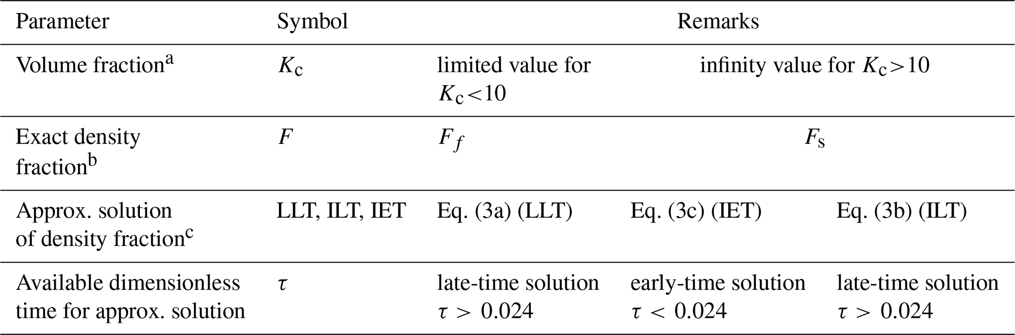
^a This defines the volumetric ratio of the total void volume of the sample cell to the pore volume of the porous samples; the classification between the limited and infinity value is proposed as 50 in the following analyses. ^b The original constitutive equation for different K_c value. ^c Equations (3a)–(3c) are three approximate solutions of density faction function F.

Based on diffusion phenomenology, Cui et al. (2009) presented two mathematical solutions similar to our Eqs. (3a) and (3c). In the work of Cui et al. (2009), however, one of late-time solution is missing, and error analyses are not provided. In addition, the lack of detailed analyses of τ and K_c in the constitutive equations will likely hinder the practical application of Eq. (3b), which is able to cover an experimental condition of small sample mass with a greater τ (further analyzed in Sect. 3). Furthermore, the early-time and late-time solution criteria are not analyzed, and the pioneering work of Cui et al. (2009) does not comprehensively assess practical applications of their two solutions in real cases, which is addressed in this study. Hereafter, we refer to the developed mathematical and experimental gas-permeability-measurement approach holistically as the gas permeability technique (GPT).

3 Practical usages of algorithms for the GPT

As aforementioned, mathematical solutions given in Eqs. (3a) and (3b) were deduced based on different values of K_c and τ, as shown in Sect. S2. This means each solution holds only under specific experimental conditions, which are mostly determined by the permeability, porosity, and mass of samples, as well as gas pressure and void volume of the sample cell. In this section, the influence of parameters K_c and τ on the solution of constitutive equation is analyzed and a specific value of dimensionless time (τ=0.024) is proposed as the criterion required to detect the early-time regime from the late-time one for the first time in the literature. We also demonstrate that the early-time solution of Eq. (3c), which has been less considered for practical applications in previous studies, is also suitable and unique under common situations. In addition, the error in the approximate solution compared to the exact solution and their capabilities are discussed, as it helps to select an appropriate mathematical solution at small τ values. Moreover, we showcase the unique applicability and feasibility of the new solution of Eq. (3b).

3.1 Sensitivity analyses of the K_c value for data quality control

To apply the GPT method, appropriately selecting the parameter K_c in Eqs. (3a)–(3c) is crucial, as it is a critical value for data quality control. The dimensionless density outside the sample, U_f, is related to K_c via Eq. (S33) in Sect. S2. One may simplify Eq. (S33) by replacing the series term with some finite positive value and set

$$\begin{array}{}\text{(4)}& U_f-{\displaystyle \frac{K_{\mathrm{c}}}{\mathrm{1}+K_{\mathrm{c}}}}>\mathrm{0}.\end{array}$$

We define $K_{\mathrm{f}}=K_{\mathrm{c}}/(\mathrm{1}+K_{\mathrm{c}})$ to interpret the density variance of the system as K_f is closely related to the dimensionless density outside the sample, U_f.

Equation (4) shows the relationship between U_f and K_c (Fig. 1). For K_c >0, K_f falls between 0 and 1. The greater the K_f value, the more insensitive to density changes the system is. For K_c equal to 50, K_f would no longer be sensitive to K_c variations as it would have already approached 98 % of the dimensionless density. This means that the U_f value needs to be greater than 0.98, and this leaves only 2 % of the fractional value of U_f available for capturing gas density change. When K_c is 100, the left fractional value of U_f would be 1 %. This would limit the number of data available (the linear range in Fig. S1) for the permeability calculation, which would complicate the data processing. Thus, for the GPT experiments, a small value of K_c (less than 10) is recommended, as K_f nearly reaches its plateau beyond K_c=10 (Fig. 1). When K_c is 10, the left fractional value of U_f is only as low as 9 %.

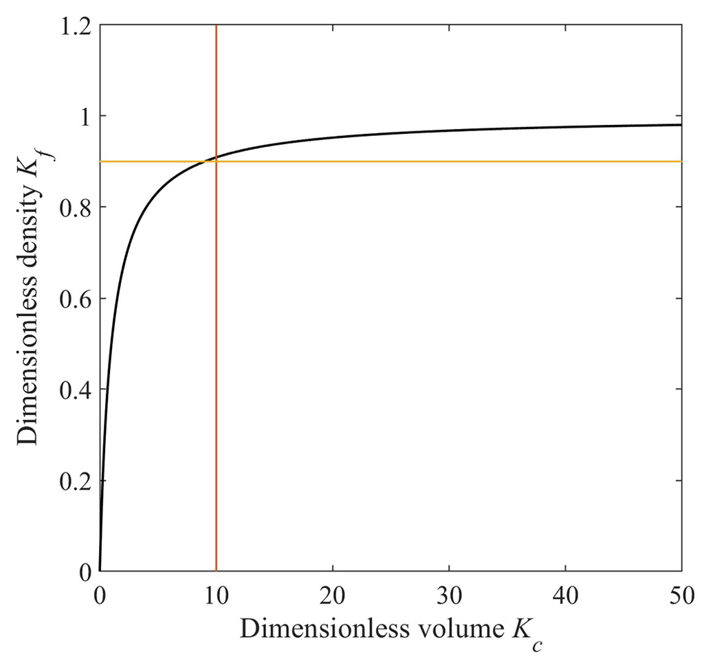
Figure 1 Dimensionless density, K_f, as a function of dimensionless volume K_c. Major variations in K_f occur for K_c<10, indicating longer gas transmission duration with more pressure decay data available for permeability derivation.

3.2 Recommendation for solution selection

The following three aspects need to be considered before selecting the appropriate solution for permeability calculation: (1) early- or late-time solutions, (2) error between the approximate and exact solutions, and (3) the convenience and applicability of solutions suitable for different experiments. We will first discuss the selection criteria for early- or late-time solutions.

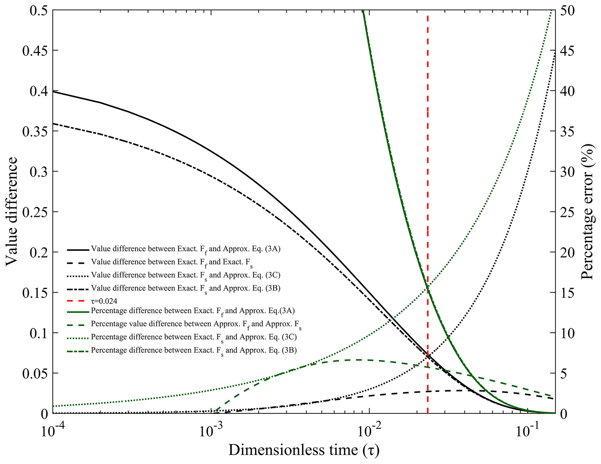
Figure 2a shows the exact solution of F_s with their approximate early- and late-time solution (Table 1). Two exact solutions of F_f where K_c equals 10 or 50 are also demonstrated in Fig. 2a. Figure 2b depicts the exact solution from F_f for different K_c values from 1 to 100 and their corresponding approximate solution for Eq. (3a). The intersection points of the solution Eqs. (3b) and (3c), namely τ=0.024 in Fig. 2a, is used for distinguishing early- and late-time solutions.

Two notable observations can be drawn from Fig. 2b. First, the approximate solution Eq. (3a) would only be applicable at late times when τ is longer than 0.024. For τ< 0.024, regardless of the K_c value, Eq. (3c) would be more precise than Eqs. (3a) and (3b) and return results close to the exact solution for both F_f and F_s. Second, the results of Eqs. (3a) and (3b) presented in Fig. 2a are similar; their difference is very small, especially for K_c>10. Due to the fact that core samples from deep wells are relatively short in length and their void volume is small (ultra-low porosity and permeability such as in mudrocks with k≤ 0.1 nd), in practice, a solution for $\mathrm{10}<K_{\mathrm{c}}<\mathrm{100}$ is the most common outcome, even if the sample cell is loaded as full as possible. Under such circumstances, the newly derived solution, Eq. (3b), becomes practical and convenient: (1) if the K_c and dimensionless time τ have not been evaluated precisely before the GPT experiment, this solution may fit most experimental situations and (2) this solution is suitable for calculation as it does not need the solution from the transcendental equation of Eq. (S30) because the denominator of α has been replaced by π. The data quality control is discussed in Sect. 4.1.

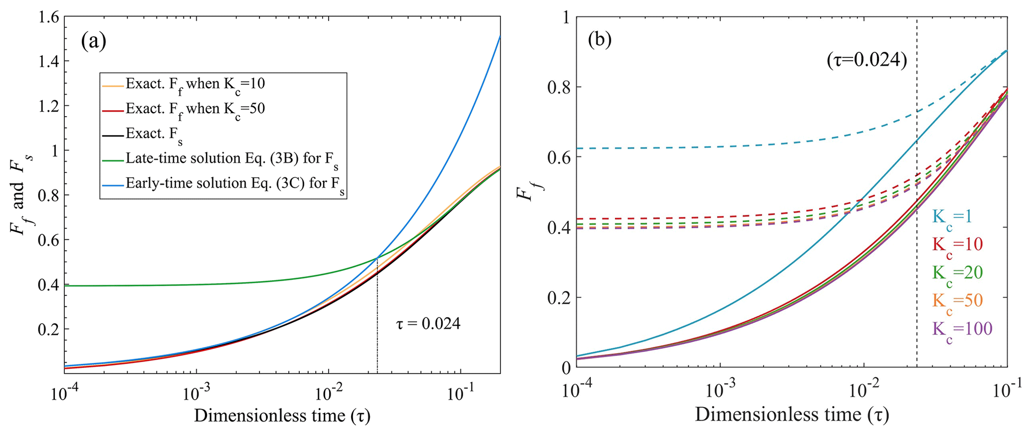
Figure 2 Three GPT solutions with different values of τ, K_c; the dashed lines are approximate solutions without a series expansion in Fig. 2b for F_f. Figure modified from Cui et al. (2009).

3.3 Applicability of the early-time solution

A small K_c value can guarantee a sufficient time for gas transfer in samples and provide enough linear data for fitting purposes. We note that the selection of the limited K_c solution of F_f, and the infinity K_c solution F_s is controlled by K_c. However, before the selection of K_c, the dimensionless time is the basic parameter to be estimated as a priori before the early- or late-time solutions are selected.

For pulse-decay methods, the early-time solution has the advantage of capturing the anisotropic information contained in reservoir rocks (Jia et al., 2019; Kamath, 1992). However, it suffers from the shortcoming of uncertainty in data for the initial several seconds, which is why it is not recommended for data processing (Brace et al., 1968; Cui et al., 2009). This is due to (1) the Joule–Thomson effect, which causes a decrease in gas temperature from the expansion, (2) kinetic energy loss during adiabatic expansion, and (3) collision between molecules and the container wall. These uncertainties normally occur in the first 10–30 s, shown in our experiments as a fluctuating period called the “early stage”.

However, the early stage present in pulse-decay experiments does not mean that the early-time solution is not applicable. We demonstrate the relationship between time and dimensionless time in Fig. 3, showing that a short dimensionless time may correspond to a long testing period of hundreds to thousands of seconds in experiments. This is particularly notable for the ultra-low-permeability samples with k≤0.1 nd and small dimensionless times τ<0.024. This situation would only be applicable to early-time solutions but with data available beyond the early stage, and it would provide available data over a long time (hundreds to thousands of seconds). For example, the early-time solution would fit ultra-low-permeability samples in 600 s for 0.1 nd and in at least 1000 s for 0.01 nd, as shown in Fig. 3 in the region below the dark line. Then, using Eq. (3c), the derived permeability would be closer to its exact solution in the earlier testing time (but still after the early stage). The mudrock samples that we tested, with results presented in Sect. 5.3, exhibit low permeabilities, approximately on the order of 0.1 nd.

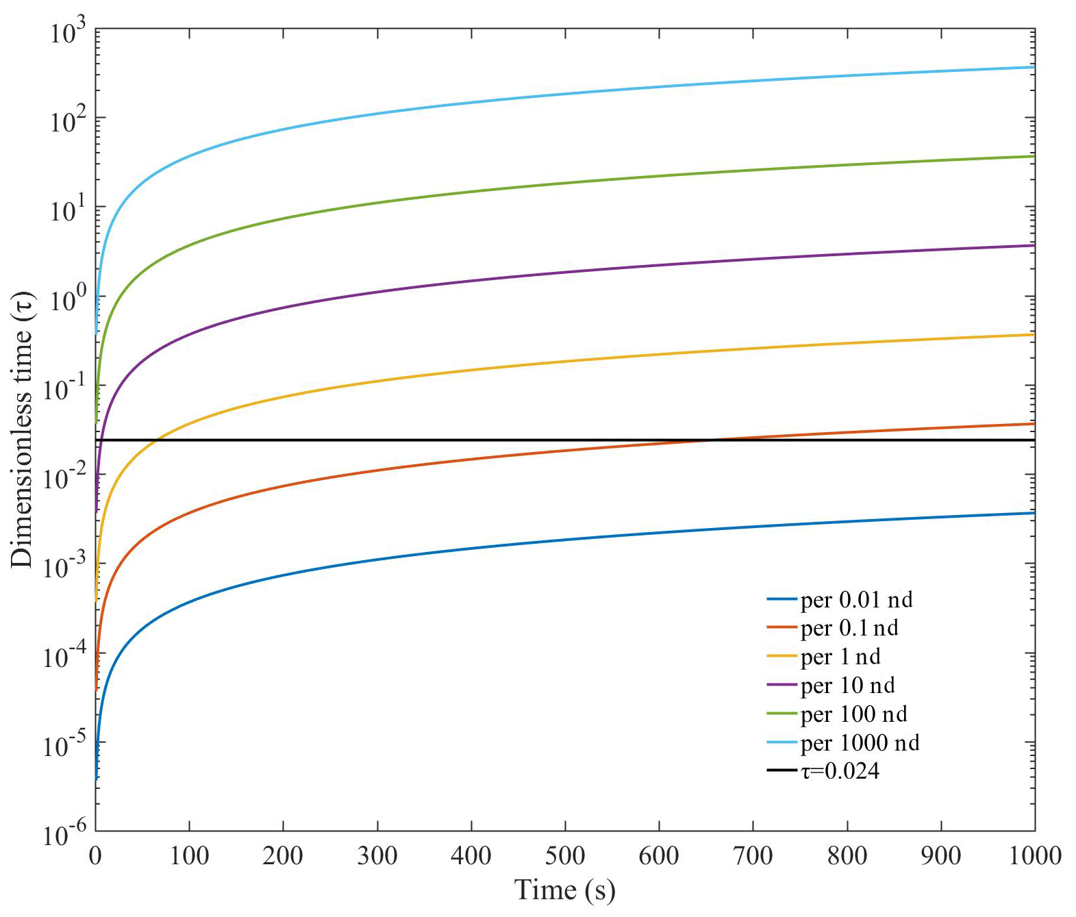
Figure 3 Dimensionless time τ versus actual time for different permeability values through Eq. (S14) using He gas, sample porosity of 5 %, and sample diameter of 2 mm, where 1 nd is nearly equal to 10⁻²¹ m².

3.4 Error analyses between exact and approximate solutions

It is unpractical to use the exact solutions with their series part to do the permeability calculation; thus, only the approximate solutions are used and the error difference between the exact and approximate solutions is discussed here. The original mathematical solutions, Eqs. (S39) and (S49), are based on series expansion. For dimensionless densities F_f and F_s in Eqs. (S39) and (S49), their series expansion terms should converge. However, the rate of convergence is closely related to the value of τ. For example, from Eq. (S30), when τ≥1, the exponent parts of U_s and U_f are at least (2n+1)π². Therefore, the entire series expansion term can be omitted without being influenced by K_c. In practical applications, the solutions given in Eqs. (3a)–(3c) are approximates without series expansion. In this study, we provide diagrams of the change in errors with dimensionless time in the presence of adsorption (Fig. 4).

For F_f, the error differences between the exact and approximate solutions are 3.5 % and 0.37 % for τ=0.05 and 0.1 when K_c=10, respectively. When τ≤0.024, the error would be greater than 14.7 %. Figure 2(b) shows that F_f can be approximated as F_s when K_c is greater than 10; the error difference between F_f and F_s is quite small at this K_c value (for K_c=10, 6.6 % is the maximum error when τ=0.01; 4.4 % when τ=0.05; and 2.9 % when τ=0.1), as shown in Fig. 4.

For F_s, the error difference is roughly the same as F_f and equal to 3.6 % for τ=0.05 and 0.38 % for τ=0.1. This verifies that newly derived Eq. (3b) is equivalent to Eq. (3a) when K_c is greater than 10. As for the evaluation of Eq. (3c), the error difference with the exact solution will increase with dimensionless time (5.1 % for τ=0.003, 9.7 % for τ=0.01, and 16 % for τ=0.024).

Figure 4 Error analyses of F_f and F_s for their exact and approximate solutions.

4 Influence of kinetic energy on gas transport behavior

4.1 Flow state of gas in granular samples

In the following, we apply the approximate solutions, Eqs. (3a)–(3c), to some detailed experimental data and determine permeability in several mudrock samples practically compatible with sample size, gases, and molecular dynamics analyses.

During the GPT, with the boundary conditions described in Sect. S2, the pressure variation is captured after gas starts to permeate the sample from the edge, and the model does not take into account the gas transport between particles or into any micro-fractures if present. Thus, the transport that conforms to the “unipore” model and occurs after the early stage (defined in Sect. 3.3) or in the “penetration zone” (the area between the two vertical lines in Fig. 5) should be used to determine the slope. Figure A2 shows how to obtain the permeability result using the applicable mathematical solutions (Eqs. 3a–3c). Figure 5 shows the pressure variance with time during the experiment using sample size from 0.34 to 5.18 mm for sample X-1 and sample X-2. From Fig. 5, the time needed to reach pressure equilibrium after the initial fluctuation stage is 20–100 s, and the penetration zone decreases with decreasing grain size over this time period.

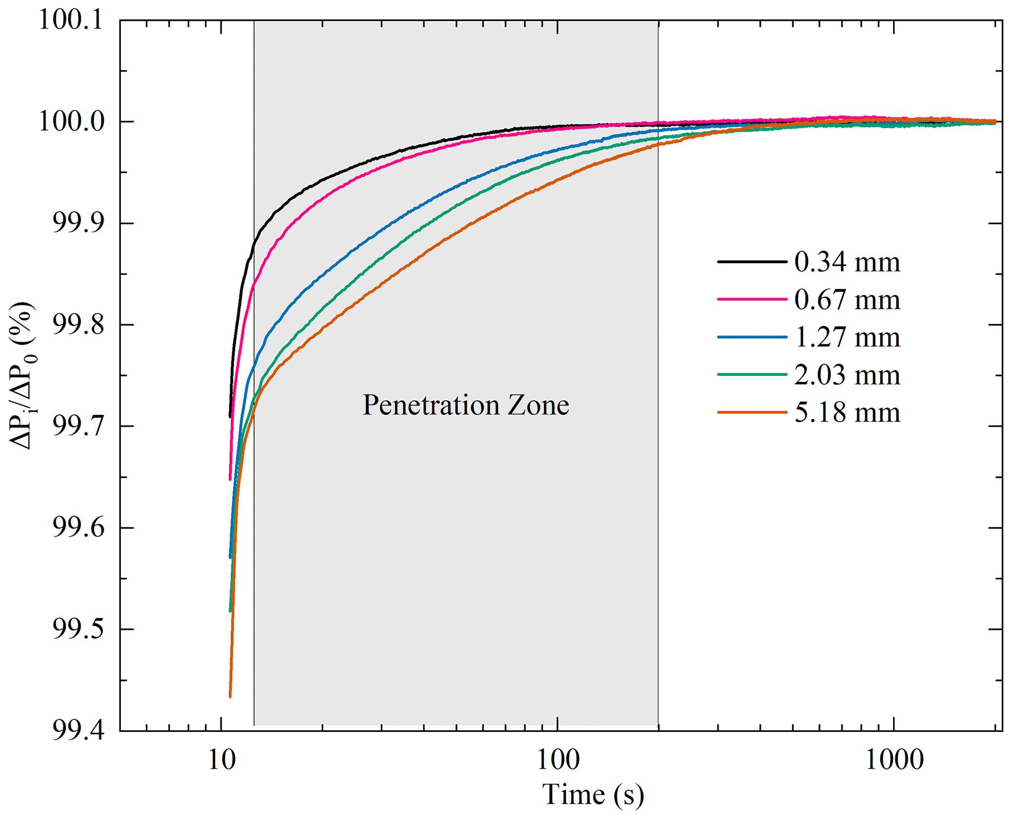
Figure 5 Fitting region (the penetration zone in the shadowed area) for mudrock sample X-1 with different granular sizes; the penetration zone illustrating the pressure gradient mainly happens at 20 to 200 s for this sample.

In fact, the penetration zone, as an empirical period, is evaluated by the pressure change over a unit of time before gas is completely transported into the inner central part of the sample to reach the final pressure. Owing to the sample size limitation, a decreasing pressure could cause multiple flow states (based on the Knudsen number) to exist in the experiment. The pressure during the GPT experiment varies between 50 and 200 psi (0.345 to 1.38 MPa). Figure 6 shows the Knudsen number calculated from different pressure conditions and pore diameters together with their potential flow state. Based on Fig. 6, the flow state of gas in the GPT experiments is mainly dominated by Fickian and transition diffusion. Essentially, the flow state change with pressure should be strictly evaluated through the Knudsen number in Fig. 6 to guarantee that the data in the penetration zone are always fitted with the GPT's constitutive equation for laminar-flow or diffusive states. This helps obtain a linear trend for ln (1−F_f) or $F_{\mathrm{s}}^{\mathrm{2}}$ versus time for low-permeability media. Experimentally, data from 30 to several hundreds of seconds are recommended for tight rocks like shales within the GPT methodology.

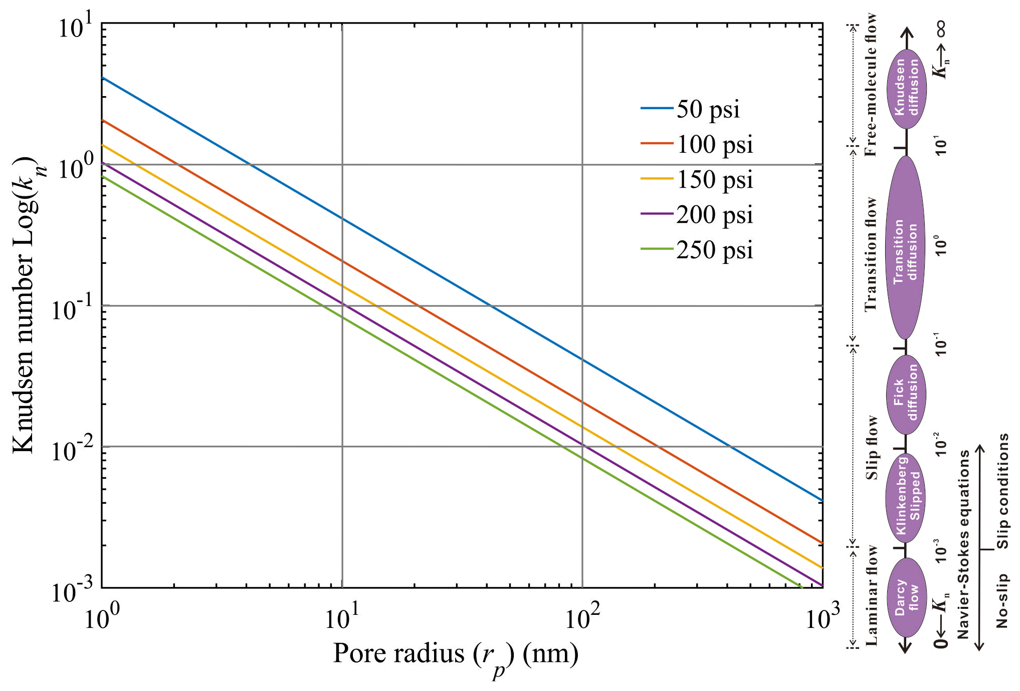
Figure 6 Flow state of gas under different testing pressures, with 145 psi being approximately equal to 1 MPa; modified from Chen and Pfender, 1983, and Roy et al., 2003.

In the GPT approach, as mentioned earlier, Eq. (S33) holds for small K_c values (e.g., <10) so that the approximately equivalent void volume in the sample cell and sample pore volume would allow for sufficient pressure drop. It also gives time and allows the probing gas to expand into the matrix pores to have a valid penetration zone and to determine the permeability. Greater values of K_c would prevent the gas flow from entering into a slippage state as the pressure difference would increase with increasing K_c. However, large pressure changes would result in a turbulent flow (Fig. 6), which would cause the flow state of gas to be no longer valid for the constitutive equation of the GPT. Overall, the GPT solutions would be applicable to gas permeability measurement, based on the diffusion-like process, from laminar flow to Fickian diffusion, after the correction of the slippage effect.

4.2 Pressure decay behavior of four different probing gases

We used three inert gases, He, N₂, and Ar, and one sorptive gas, CO₂ (Busch et al., 2008), to compare the pressure drop behavior for the sample size with an average granular diameter of 0.675 mm. Results for the mudrock sample X-2 are presented in Fig. 7. Among the three inert gases, helium and argon required the shortest and longest time to reach pressure equilibrium (i.e., He <N₂<Ar). In terms of pressure drop, argon exhibited the most significant decrease. In a constant-temperature system, the speed (or rate) at which gas molecules move is inversely proportional to the square root of their molar masses. Hence, it is reasonable that helium (with the smallest kinetic diameter of 0.21 nm) has the shortest equilibrium time. However, the pressure drop is more critical than the time needed to reach equilibrium for the GPT, as the equilibrium time does not differ much (basically within 10 s for a given sample weight, except for the adsorptive CO₂). Argon may provide a wider range of valid penetration zones given its longest decay time (when excluding the adsorbed gas CO₂).

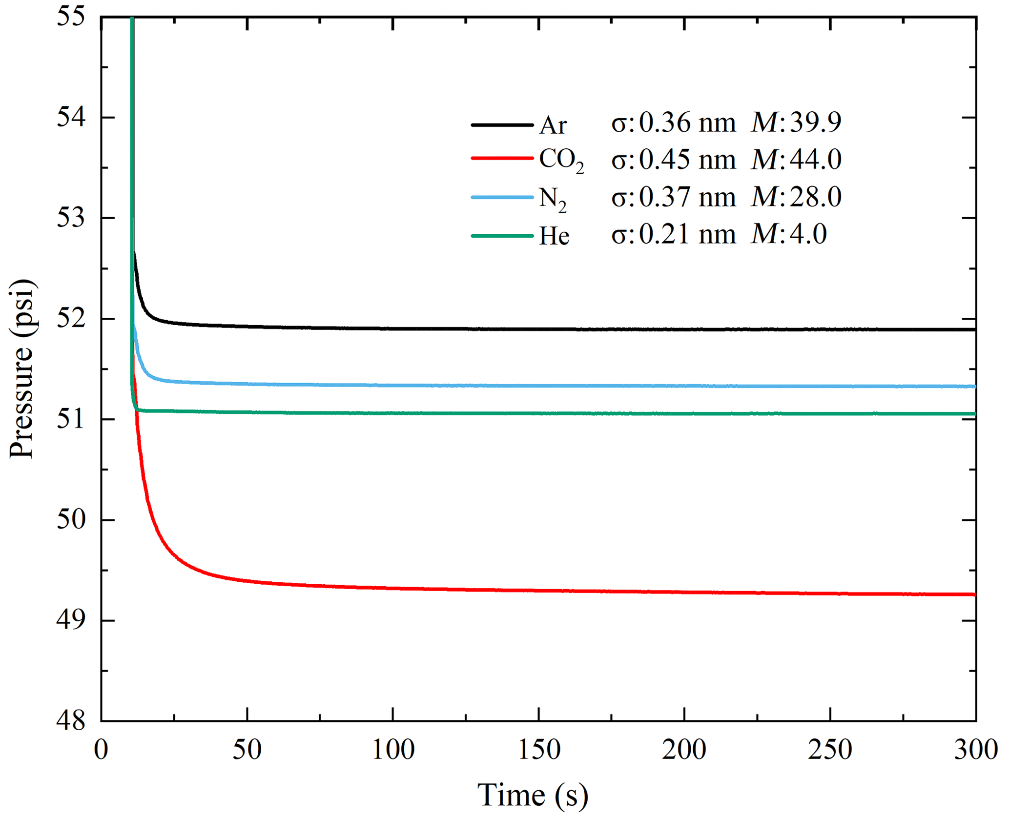
Figure 7 Measured pressure decay curves from mudrock sample X-2 for gases of different molecular diameters σ and molecular weights M (g mol⁻¹); decay happened at around 50 psi (approximately 0.345 MPa)

Figure 7 shows that the pressure decay curve of the adsorptive gas CO₂ is different from those of the inert gases used in this study. CO₂ has a slow equilibrium process due to its large molar mass and the greatest pressure drop among the four gases due to its adsorption effect. This additional flux needs to be taken into account to obtain an accurate transport coefficient. Accordingly, multiple studies including laboratory experiments (Pini, 2014) and long-term field observations (Haszeldine et al., 2006; Lu et al., 2009) were carried out to assess the sealing efficiency of mudrocks for CO₂ storage. In fact, the GPT offers a quick and effective way to identify the adsorption behavior of different mudrocks for both laminar-flow and diffusion states.

4.3 Pressure decay behavior for different granular sizes

We compared the pressure drop behavior of gas in the mudrock sample X-1 with different granular sizes (averaging from 0.34 to 5.18 mm) using the same sample weight and K_c. Results based on the experimental data shown in Fig. 8 indicate that a larger-sized sample would provide more data to be analyzed for determining the permeability. This is because the larger the granular size, (1) the larger the pressure drop and (2) the greater the decay time, as Fig. 8 demonstrates. This is consistent with the simulated results reported by Profice et al. (2012).

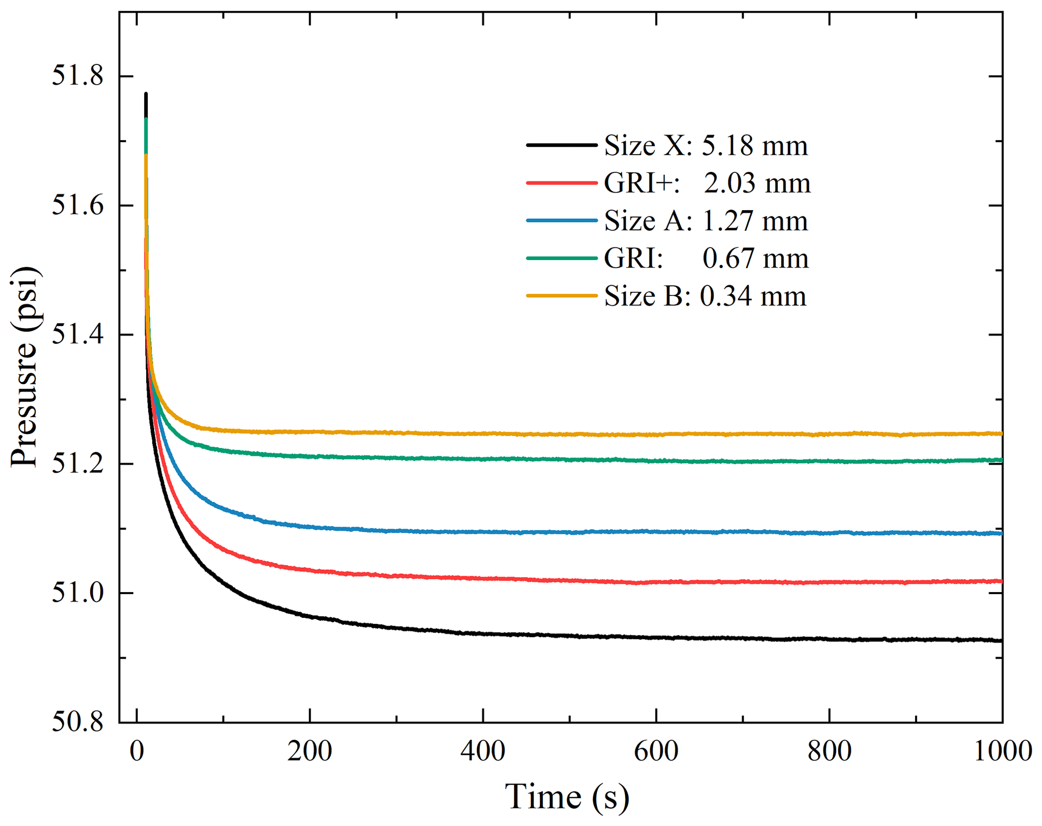
Figure 8 Pressure decay curves (50 psi equals approximately 0.345 MPa) measured by helium on sample X-1 with five different granular sizes. The intra-granular porosity was 5.8 %, independently measured by mercury intrusion porosimetry.

Table 2 Permeability results from the methods of GPT and SMP-200 for X-1.

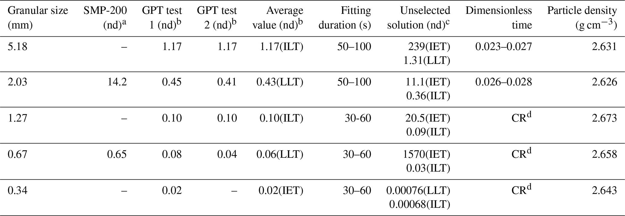
^a The results are from the SMP-200 using the GRI default method. ^b The results are from the GPT method we proposed. ^c The result which failed the criteria of dimensionless time. ^d CR means conflicting results, as the verified dimensionless time fails to corroborate the early- or late-time solutions derived from the calculated permeability. For example, the verified dimensionless time would be >0.024 using the early-time solution result and vice versa.

As reported in Table 2, the permeability values measured by the GPT method are 1 or 2 orders of magnitude greater than those measured by the SMP-200 instrument. The built-in functions of SMP-200 can only be used for two default granular sizes (500–841 µm for GRI and 1.70–2.38 mm for what we call GRI+) to manually curve-fit the pressure decay data and determine the permeability. The GRI method built in the SMP-200 only suggests the fitting procedure for data processing without publicly available details on the underlying mathematics. The intra-granular permeabilities of mudrock sample X-1 vary from 0.02 to 1.17 nd for five different granular sizes using the GPT. With the same pressure decay data selected from 30 to 200 sec, the permeability results for GRI and GRI+ sample sizes from the SMP-200 fitting are 0.65 and 14.2 nd as compared to 0.06 and 0.43 nd determined by the GPT using the same mean granular size. Our results are consistent with those reported by Peng and Loucks (2016), who found differences of 2 to 3 orders of magnitude between the GPT and SMP-200 methods (Peng and Loucks, 2016).

There are several issues associated with granular samples with diameters smaller than, on average, 1.27 mm. First, the testing duration is short, and second, there is not sufficient pressure variation analyzed in Fig. 8. Both may cause significant uncertainties in the permeability calculation and, therefore, make samples with diameters smaller than 1.27 mm unfavorable for the GPT method, particularly ultra-tight (sub-nanodarcy levels) samples as there is almost no laminar-flow or diffusion state to be captured. The greater pressure drop for larger-sized granular samples would result in greater pressure variation and wider data region compared to smaller granular sizes (see Figs. 6 and 9). Although samples of large granular sizes may potentially contain micro-fractures, which complicate the determination of true matrix permeability (Heller et al., 2014), the versatile GPT method can still provide size-dependent permeabilities for a wide range of samples (e.g., from sub-millimeter to 10 cm diameter full-size cores) (Ghanbarian, 2022a, b). In addition, the surface roughness of large grains may also complicate the determination of permeability, which requires attention (Devegowda, 2015; Rasmuson, 1985; Ruthven and Loughlin, 1971). Overall, our results demonstrated that sample diameters larger than 2 mm are recommended for the GPT to determine the nanodarcy permeability of tight mudrocks, while smaller sample sizes may produce uncertain results.

4.4 Practical recommendations for the holistic GPT

Here, we evaluate the potential approximate solution for tight rock samples using frequently applied experimental settings by considering the critical parameters, such as sample mass, porosity, and estimated permeability (as compiled in Fig. 9 showing the dimensionless time versus porosity). Based on the results presented in Figs. 3 and 6, only t<200 s is dominant and critical for the analyses of dimensionless time and penetration zone. Thus, we take 200 s and use helium to calculate the dimensionless time. Another critical parameter to ensuring sufficient decay data is a sample diameter of greater than 2 mm. Thus, we only show the dimensionless time versus porosity for sample diameters greater than the criteria of 2 mm.

Figure 9 demonstrates that the sample permeability has dominant control on early- or late-solution selection, and we decipher a concise criterion for the selection of the three solutions. We classify the dimensionless time versus porosity relationship into three cases. First, among the curves shown in Fig. 9, only that corresponding to k=0.1 nd and sample diameter of 2 mm stays below the dashed line representing τ=0.024. Therefore, the early-time solution is appropriate for tight samples with permeabilities less than 0.1 nd (as shown in the analyses of Sect. 4.3, which also conforms to the situation of the molecular sieve sample that we tested in Sect. S3). Second, for permeabilities greater than 10 nd (the curve is above the line of τ=0.024), the newly derived late-time solution, Eq. (3b), is recommended as it is more convenient for mathematical calculation without the consideration of transcendental functions. The reason is that the sample cell can be filled as much as possible (∼90 % of the volume) with samples and solid objects. However, as the tight rock hardly presents a large value of porosity, it is difficult to achieve a small K_c value, with an inconsequential influence between Eqs. (3b) and (3a). Lastly, in the case of permeability around 1 nd, the value of porosity would be critical in the selection of the early- or late-time solutions, as shown in Fig. 9.

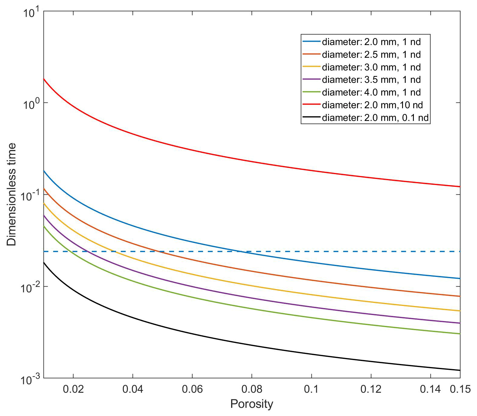
Figure 9 Holistic GPT used to explore the appropriate solution based on diameter, permeability, and porosity of samples. The legend shows the diameter of granular sample and permeability, along with a dashed line for a dimensionless time of 0.024, while regions above and below this value fit for the late- and early-time solutions, respectively (1 nd is nearly equal to 10⁻²¹ m²).

5 Conclusions

In the present work, we solved a fluid flow state equation in granular porous media and provided three exact mathematical solutions along with their approximate ones for practical applications of low-permeability measurements. The mathematical solutions for the transport coefficient in the GPT were derived for a spherical coordinate system, applicable from laminar flow to slippage-corrected Fickian diffusion. Of the three derived solutions, the early-time solution is valid when the gas storage capacity K_c approaches infinity, while the other two are late-time solutions, valid when K_c is either small or tends towards infinity. We evaluated the derived solutions for a systematic measurement of ultra-low permeabilities in granular media and crushed rocks using experimental methodologies with the data processing procedures. We determined the error for each solution by comparing with the exact solutions presented in the Supplement. The applicable conditions for such solutions of the GPT were investigated, and we provided the selection strategies for three approximate solutions based on the range of sample permeability. In addition, a detailed utilization of GPT was given to increase confidence in the GPT method through the molecular sieve sample, as it allows for a rapid permeability test for ultra-tight rock samples in just tens to hundreds of seconds, with good repeatability.

Appendix A: Nomenclature

Bij	Correction parameter for viscosity, constant
ct	Fluid compressibility, Pa−1
Ff	Uptake rate of gas outside the sample, dimensionless
Fs	Uptake rate in the sample, dimensionless
f1	Intercept of Eq. (S40), constant
Ka	Apparent transport coefficient defined as Eq. (S9), m2 s−1
Kc	Ratio of gas storage capacity of the total void volume of the system to the pore (including adsorptive and
	non-adsorptive transport) volume of the sample, fraction
Kf	Initial density state of the system, fraction
k	Permeability, m2
ks	Permeability defined as Eq. (S8), m2 (Pa s)−1
L	Coefficient, unit for certain physical transport phenomenon
M	Molar mass, kg kmol−1
Mm	Molar mass of the mixed gas, kg kmol−1
Mi,j	Molar mass for gas i or j, kg kmol−1
Ms	Total mass of sample, kg
N	Particle number, constant
p	Pressure, Pa
pcm	Virtual critical pressure of mixed gas, Pa
pp	Pseudo-pressure from Eq. (S1), Pa s−1
Ra	Particle diameter of sample, m
R	Universal gas constant, 8.314 J (mol K)−1
r	Diameter of sample, m
s1	Slope of Eq. (S40), constant
s2	Slope of function Ln(1−Fs), constant
s3	Slope of function $F_{\mathrm{s}}^{\mathrm{2}}$, constant
T	Temperature, K
Tcm	Virtual critical temperature for mixed gas, K
t	Time, s
Uf	Dimensionless density of gas outside the sample, dimensionless
Us	Dimensionless density in grain, dimensionless
U∞	Maximum density defined as Eq. (S37), dimensionless
V1	Cell volume in upstream of pulse-decay method, m3
V2	Cell volume in downstream of pulse-decay method, m3
Vb	Bulk volume of sample, m3
Vc	Total system void volume except for sample bulk volume, m3
$\stackrel{\mathrm{‾}}{v}$	Darcian velocity in pore volume of porous media, m s−1
X	Pressure force, Pa
yi,j	Molar fraction for gas i or j, fraction
z	Gas deviation (compressibility) factor, constant

Appendix B: Greek letters

αn	nth root of Eq. (S30), constant
μ	Dynamic viscosity, Pa s or N s m−2
μi,j	Dynamic viscosity for gas i or j, Pa s or N s m−2
μmix	Dynamic viscosity of mixture gas, Pa s or N s m−2
μp	Correction term for the viscosity with pressure, Pa s or N s m−2
ξ	Dimensionless radius of sample, dimensionless
ρ	Density of fluid, kg m−3
ρ0	Average gas density on the periphery of sample, kg m−3
ρ1	Gas density in reference cell, kg m−3
ρ2	Gas density in sample cell, kg m−3
ρb	Average bulk density for each particle, kg m−3
ρf	Density of gas changing with time outside sample, kg m−3 s−1
ρf∞	Maximum value of ρf defined as Eq. (S38), kg m−3 s−1
ρp	Pseudo-density from Eq. (S1), kg m−3 s−1
ρs	Density of gas changing with time in sample, kg m−3 s−1
ρps	Pseudo-density of gas changing with time in sample, kg m−3 s−1
ρpf	Pseudo-density of gas changing with time outside sample, kg m−3 s−1
ρp2	Initial pseudo-density of gas in sample, kg m−3 s−1
ρp0	Average pseudo-density of gas on sample periphery, kg m−3 s−1
ρrm	Relative density to the mixed gas, kg m−3 s−1
ρsav	Average value of ρsr defined as Eq. (S47), kg m−3 s−1
ρsr	Average value of pseudo-density of sample changing with diameter, kg m−3 s−1
ρs∞	Maximum value of ρsr defined as Eq. (S46), kg m−3 s−1
τ	Dimensionless time, dimensionless
ϕ	Sample porosity, fraction
ϕf	Total porosity (${\mathit{\varphi }}_{\mathrm{f}}={\mathit{\varphi }}_{\mathrm{a}}+{\mathit{\varphi }}_{\mathrm{b}}$) occupied by both free and adsorptive fluids, fraction