Inferring heavy tails of flood distributions through hydrograph recession analysis

Floods are often disastrous due to underestimation of the magnitude of rare events. Underestimation commonly happens when the magnitudes of floods follow a heavy-tailed distribution, but this behavior is not recognized and thus neglected for flood hazard assessment. In fact, identifying heavy-tailed flood behavior is challenging because of limited data records and the lack of physical support for currently used indices. We address these issues by deriving a new index of heavy-tailed flood behavior from a physically based description of streamflow dynamics. The proposed index, which is embodied by the hydrograph recession exponent, enables inferring heavy-tailed flood behavior from daily flow records, even of short length. We test the index in a large set of case studies across Germany encompassing a variety of climatic and physiographic settings. Our findings demonstrate that the new index enables reliable identification of cases with either heavy- or non-heavy-tailed flood behavior from daily flow records. Additionally, the index suitably estimates the severity of tail heaviness and ranks it across cases, achieving robust results even with short data records. The new index addresses the main limitations of currently used metrics, which lack physical support and require long data records to correctly identify tail behaviors, and provides valuable information on the tail behavior of flood distributions and the related flood hazard in river basins using commonly available discharge data.

1 Introduction

Floods remain the leading natural hazards worldwide, directly threatening the livelihoods of at least one-fifth of the world's population (McDermott, 2022; Rentschler et al., 2022) and causing enormous economic losses (Bevere and Remondi, 2022). Flood frequency analysis is a central and commonly used tool to assess the hazard of extreme floods, which is usually achieved by parametrically fitting a selected probability distribution on flow maxima, e.g., the annual maximum flood (Villarini and Smith, 2010), or peak-over-threshold series (Pan et al., 2022). Selecting a suitable distribution that can properly describe (or predict) the extreme events is, however, often challenging due to the notable uncertainties caused by the lack of data in the maxima approach (Papalexiou and Koutsoyiannis, 2013; Hu et al., 2023). The upper-tailed behavior (which we will refer to as tail behavior throughout the paper for simplicity) of the underlying distribution critically determines the accuracy of the extreme events. If a catchment has the potential for heavy-tailed flood behavior but this characteristic is not accounted for in the selection of probability distributions, the probability of extreme floods may be significantly underestimated (Merz et al., 2022). This can lead to disastrous floods and severe damages (Merz et al., 2021). Therefore, correctly identifying the tail behavior of flood distributions is crucial for avoiding potential underestimation of extreme floods.

The tail heaviness of an empirical distribution is typically estimated through graphical or statistical methods, although both methods have limitations. Graphical methods, such as log–log plots (Beirlant et al., 2004), generalized Hill ratio plots (Resnick, 2007; El Adlouni et al., 2008), and mean excess functions (Embrechts et al., 1997; Nerantzaki and Papalexiou, 2019), are less objective and efficient for large-scale analyses (Cooke et al., 2014). In contrast, statistical methods, such as parametric metrics that fit distributions to the observed data (Papalexiou et al., 2013; Seckin et al., 2011; Smith et al., 2018; Villarini and Smith, 2010), and non-parametric metrics, like the upper-tail ratio (Lu et al., 2017; Smith et al., 2018; Villarini et al., 2011; Wang et al., 2022), Gini index (Eliazar and Sokolov, 2010; Rajah et al., 2014), and obesity index (Cooke and Nieboer, 2011; Sartori and Schiavo, 2015), provide more objective insights into tail behavior. However, obtaining reliable estimates from these methods requires long data records (Papalexiou and Koutsoyiannis, 2013), a condition which is often not fulfilled globally (Lins, 2008) and may cause bias when comparing data across sites with different record lengths (Cunderlik and Burn, 2002; Wietzke et al., 2020). To reduce uncertainty, especially in estimating extremes, recent studies recommend analyzing ordinary dynamics instead of focusing solely on maximum values (Marani and Ignaccolo, 2015; Mushtaq et al., 2022) and investigating the underlying factors that contribute to extreme events (Wilson and Toumi, 2005; Tarasova et al., 2020; Merz et al., 2022).

Floods are often triggered by rainfall, and numerous studies have contributed to an improved understanding of rainfall extremes (e.g., Koutsoyiannis, 2004a, b, 2022; Martinez-Villalobos and Neelin, 2021). However, several studies have clarified that rainfall extremes do not necessarily translate into flood extremes (e.g., McCuen and Smith, 2008; Pall et al., 2011; Hall et al., 2014; Archfield et al., 2016; Rossi et al., 2016; Zhang et al., 2016; Hodgkins et al., 2017; Sharma et al., 2018). For instance, McCuen and Smith (2008) showed that skewed rainfall distributions do not always produce skewed flood distributions. They proposed that catchment responses and storage dynamics contribute to the generation of flood extremes. This view was supported by Sharma et al. (2018), who argued that, despite a significant increase in rainfall extremes, a corresponding increase in flood extremes was not observed. The thorough review of Merz et al. (2022) concluded that, while rainfall plays a primary role in generating runoff, the emergence of flood extremes is largely determined by catchment responses and water balance. Given these premises, an appropriate approach for describing runoff and its extremes should be rooted in the dynamics of soil moisture and rainfall–runoff processes within catchments.

This study aims to investigate whether a suitable descriptor of the tail behavior of flood distributions exists by exploring the intrinsic hydrological dynamics of the flow regime. Currently, to the best of our knowledge, widely used metrics for tail behavior estimation of flood distributions do not incorporate such a physical description. Instead of proposing a standard probability distribution for streamflow or floods, as done by several others before (e.g., Vogel et al., 1993; Merz and Thieken, 2009; Saf, 2009; Rahman et al., 2013; Kousar et al., 2020; Dimitriadis et al., 2021), our goal is to test against data the inference capabilities of the proposed index of heavy-tailed behavior identified from a description of runoff generation processes in river basins. As mentioned earlier, classical fitting methods for assessing tail behavior are known to be highly sensitive to the specific data record used for fitting. This study presents an alternative method for inferring heavy-tailed flood behavior by characterizing well the underlying dynamics of the system which are responsible for the emergence of tail behavior. This approach has the potential to enhance the accuracy and reliability of tail behavior estimation for flood distributions because it does not solely rely on fitting the available datasets.

To achieve this, we begin the analysis with a mechanistic description of hydrological processes. We subsequently distinguish between the key processes generating heavy- and non-heavy-tailed behavior of flood distributions and propose a physical descriptor for heavy-tailed flood behavior which is based on common streamflow dynamics. We verify its ability to identify heavy-tailed flood behavior and its robustness in datasets with decreasing lengths through numerous case studies across Germany encompassing various climate and physiographic characteristics. This confirms the practical transferability and stability of the descriptor.

2 Identifying tail behavior from hydrological dynamics

We describe key hydrologic processes occurring at the catchment scale and the resulting probability distributions of streamflow and floods by means of the PHysically-based Extreme Value (PHEV) distribution of river flows (Basso et al., 2021). This framework is grounded in a well-established mathematical description of precipitation, soil moisture, and runoff generation in river basins (Laio et al., 2001; Porporato et al., 2004; Botter et al., 2007b, 2009). Rainfall is described as a marked Poisson process with frequency λ_p [T⁻¹] and exponentially distributed depths with average α [L]. Soil moisture increases due to rainfall infiltration and decreases due to evapotranspiration. The latter is represented by a linear function of soil moisture between the wilting point and an upper critical value expressing the water-holding capacity of the root zone. Runoff pulses occur with frequency λ<λ_p when the soil moisture exceeds the critical value. These pulses replenish a single catchment storage, which drains according to a nonlinear storage–discharge relation. The related hydrograph recession is described via a power-law function with exponent a [–] and coefficient K [L^1−a/T^2−a] (Brutsaert and Nieber, 1977), which allows for mimicking the joint effect of different flow components (Basso et al., 2015). The description of daily rainfall as a Poisson process is grounded in extensive literature (e.g., Cox and Isham, 1988; Rodriguez-Iturbe et al., 1999; Porporato et al., 2004; Yunus et al., 2017). Some studies (e.g., Papalexiou et al., 2013), however, argued that heavier-tailed distributions better represent the tail of rainfall records. The chosen rainfall description may thus affect the resulting statistical properties of streamflow. Nevertheless, a recent review of the state of the art (Merz et al., 2022) on this topic stresses that, although the tail of precipitation matters, this is not the dominant factor which determines the tail of streamflow and flood distributions, as is the case with catchment processes. The adopted description of runoff generation and streamflow dynamics was successfully tested in a variety of hydro-climatic and physiographic conditions (Arai et al., 2020; Botter et al., 2007a, 2010; Ceola et al., 2010; Doulatyari et al., 2015; Mejía et al., 2014; Müller et al., 2014, 2021; Pumo et al., 2014; Santos et al., 2018; Schaefli et al., 2013).

PHEV provides a set of consistent expressions (Basso et al., 2021) for the probability distributions of daily streamflow, ordinary peak flows (i.e., local flow peaks occurring as a result of streamflow-producing rainfall events; sensu Miniussi et al., 2020), and floods (i.e., flow maxima in a certain time frame; Basso et al., 2016). The probability distribution of daily streamflow q can be expressed as follows (Botter et al., 2009):

$$\begin{array}{}\text{(1)}& p\left(q\right)=C_{\mathrm{1}}\cdot q^{-a}\left(e^{\frac{-\mathrm{1}}{\mathit{\alpha }K(\mathrm{2}-a)}\cdot q^{\mathrm{2}-a}}\right)\left(e^{\frac{\mathit{\lambda }}{K(\mathrm{1}-a)}\cdot q^{\mathrm{1}-a}}\right),\end{array}$$

where C₁ is a normalization constant. The probability distribution of ordinary peak flows and flow maxima can be expressed as p_j(q) and p_M(q), respectively (Basso et al., 2016):

$$\begin{array}{}\text{(2)}& {\displaystyle }& {\displaystyle }{p}_j(q=C_{\mathrm{2}}\cdot q^{\mathrm{1}-a}\cdot e^{-\frac{q^{\mathrm{2}-a}}{\mathit{\alpha }K(\mathrm{2}-a)}\cdot e^{q^{\mathrm{1}-a}K(\mathrm{1}-a)}},\text{(3)}& {\displaystyle }& {\displaystyle }{p}_M\left(q\right)=p_j\left(q\right)\cdot \mathit{\lambda }\mathit{\tau }\cdot e^{-\mathit{\lambda }\mathit{\tau }\cdot D_j\left(q\right)},\end{array}$$

where $D_j\left(q\right)=\underset{q}{\overset{\mathrm{\infty }}{\int }}{p}_j\left(q\right)\mathrm{d}q$, τ [day] is the duration of the considered time frame, and C₂ is a normalization constant.

Notably, the mathematical expression of flow distributions provided by the PHEV framework is composed of a power law and two stretched exponential distributions, although it is important to note that PHEV does not assume a specific probability distribution for streamflow representation. The use of stretched exponential distributions introduces greater flexibility in capturing tail behavior compared to the exponential distribution. Depending on its parameter values, the stretched exponential distribution can display either light-tailed or heavy-tailed behavior, whereas the exponential distribution consistently exhibits a light-tailed behavior. In fact, recent studies (Basso et al., 2016, 2021, 2023) have substantiated and documented PHEV's efficacy in representing high-flow behaviors.

Taking the limit of Eq. (1) for $q\to +\mathrm{\infty }$ provides indications of the tail behavior of the flow distribution (Basso et al., 2015). This is determined by the three terms in the equation, namely, one power law and two exponential functions, which behave differently depending on the value of the hydrograph recession exponent a (Eq. 4; notice that a>1 in most river basins; Biswal and Kumar, 2014; Tashie et al., 2020b).

$$\begin{array}{}\text{(4)}& \begin{array}{rl}& \underset{q\to +\mathrm{\infty }}{\lim }p\left(q\right)=\\ & {\left\{\begin{array}{l}{C}_{\mathrm{1}}\cdot \underset{\mapsto \mathrm{0}}{\underbrace{\stackrel{\mapsto \mathrm{0}}{\overbrace{q^{-a}}}}}\underset{\mapsto e^{\mathrm{0}}=\mathrm{1}}{\underbrace{\stackrel{\mapsto \mathrm{0}}{\overbrace{\left(e^{\frac{-\mathrm{1}}{\mathit{\alpha }K(\mathrm{2}-a)}\cdot q^{\mathrm{2}-a}}\right)}}}}\underset{\mapsto e^{\mathrm{0}}=\mathrm{1}}{\underbrace{\stackrel{\mapsto e^{\mathrm{0}}=\mathrm{1}}{\overbrace{\left(e^{\frac{\mathit{\lambda }}{K(\mathrm{1}-a)}\cdot q^{\mathrm{1}-a}}\right)}}}}\end{array}\right\}}_{\mathrm{for}a>\mathrm{2}}^{\mathrm{for}\mathrm{1}<a<\mathrm{2}}\end{array}\end{array}$$

When $\mathrm{1}<a<\mathrm{2}$, the last term on the right-hand side converges to a constant value of 1 as q increases, thereby no longer influencing how the distribution decreases toward zero. The first two terms instead decrease toward zero, affecting how the probability decreases for increasing values of q. The tail behavior is, in this case, determined by both a power law and a stretched exponential function, indicating that the probability decreases faster than a stretched exponential but slower than a power law. When a>2, both the stretched exponential terms converge to a constant value of 1 as q increases and thus no longer influence how the probability decreases toward zero. In this case, the tail of the distribution is solely determined by the power-law function. Despite being aware that several definitions of heavy-tailed distributions exist (El Adlouni et al., 2008; Vázquez et al., 2006), in the remainder of the paper we refer to distributions which exhibit a power-law tail that is heavy tailed.

From the above derivations, the hydrograph recession exponent emerges as a key index of the tail behavior of streamflow distributions, which will be heavy tailed for values of a>2. We apply the same analyses to infer the tail behavior of the probability distributions of ordinary peak flows and floods by taking the limit of $q⟶+\mathrm{\infty }$ for both Eqs. (2) and (3). Because $D_j\left(q\right)=\underset{\mathrm{\infty }}{\overset{\mathrm{\infty }}{\int }}{p}_j\left(q\right)\mathrm{d}q=\mathrm{0}$, Eqs. (2) and (3) can be transformed into the following: (set C₃=λτC₂)

$$\begin{array}{}\text{(5)}& {\displaystyle }\begin{array}{rl}\underset{q\to +\mathrm{\infty }}{\lim }{p}_j\left(q\right)& =\\ & {\left\{\begin{array}{l}{C}_{\mathrm{2}}\cdot \underset{\mapsto \mathrm{0}}{\underbrace{\stackrel{\mapsto \mathrm{0}}{\overbrace{q^{\mathrm{1}-a}}}}}\underset{\mapsto e^{\mathrm{0}}=\mathrm{1}}{\underbrace{\stackrel{\mapsto \mathrm{0}}{\overbrace{\left(e^{\frac{-\mathrm{1}}{\mathit{\alpha }K(\mathrm{2}-a)}\cdot q^{\mathrm{2}-a}}\right)}}}}\end{array}\right\}}_{\mathrm{for}a>\mathrm{2}}^{\mathrm{for}\mathrm{1}<a<\mathrm{2}},\end{array}\text{(6)}& {\displaystyle }\begin{array}{rl}\underset{q\to +\mathrm{\infty }}{\lim }{p}_M\left(q\right)& =\\ & {\left\{\begin{array}{l}{C}_{\mathrm{3}}\cdot \underset{\mapsto \mathrm{0}}{\underbrace{\stackrel{\mapsto \mathrm{0}}{\overbrace{q^{\mathrm{1}-a}}}}}\underset{\mapsto e^{\mathrm{0}}=\mathrm{1}}{\underbrace{\stackrel{\mapsto \mathrm{0}}{\overbrace{\left(e^{\frac{-\mathrm{1}}{\mathit{\alpha }K(\mathrm{2}-a)}\cdot q^{\mathrm{2}-a}}\right)}}}}\end{array}\right\}}_{\mathrm{for}a>\mathrm{2}}^{\mathrm{for}\mathrm{1}<a<\mathrm{2}}.\end{array}\end{array}$$

Notably, we observe that the same critical value of the recession exponent equal to 2 also separates the absence and presence of heavy-tailed behavior in these cases. Therefore, we propose the hydrograph recession exponent a as an indicator of heavy-tailed flood behavior based on the description of hydrological processes embedded in the PHysically-based Extreme Value model. We test its capability to correctly predict such behavior in Sect. 4 and discuss the results in Sect. 5.

3 Data and parameter estimation

To test the proposed index of heavy-tailed flood behavior (i.e., the hydrograph recession exponent a), we use daily streamflow records of 98 gauges across Germany (Appendix B). The analyzed river basins encompass a variety of climate and physiographic settings (Tarasova et al., 2020). Their areas range from 110 to 23 843 km², with a median value of 1195 km². The length of the streamflow records range from 35 to 63 years, with a median value of 58 years (in between 1951–2013). We perform all analyses on a seasonal basis (winter: December–February, spring: March–May, summer: June–August, fall: September–November) to account for the seasonality of hydrograph recessions (Tashie et al., 2020b) and flood distributions (Durrans et al., 2003). We term the analysis of a given river gauge during a season as a case study. We select gauges for which processes driving streamflow dynamics are reasonably consistent with the adopted theoretical framework. Hence, we discard gauges affected by large dams, reservoirs (Lehner et al., 2011), and anthropogenic flow disturbances (based on visual examination; Tarasova et al., 2018). Case studies with strong snowfall (during a season), for which the average daily temperature is below 0 ^∘C during precipitation events for over 50 % of a season, are also discarded (i.e., only the affected season is removed from the analyses). This results in an overall number of 386 case studies, including 97 case studies in spring, 96 in summer, 98 in fall, and 95 in the winter season.

The proposed index is derived from hydrograph recession analysis. The hydrograph recession is typically described by a power-law relationship between the rate of change of streamflow in time, $\mathrm{d}q/\mathrm{d}t$, and the magnitude of streamflow q (Brutsaert and Nieber, 1977). This approach is widely recognized as a standard practice in the field (e.g., Wittenberg, 1999; Biswal and Marani, 2010; Krakauer and Temimi, 2011; Troch et al., 2013; Pauritsch et al., 2015; Jepsen et al., 2016; Sharma et al., 2023). Recent studies have suggested estimating this power-law relationship for individual recession events rather than aggregating them in order to enhance the representation of observed recession behavior. Fitting a single power-law relationship to the aggregated data points from all observed recessions often results in an underestimation of the observed hydrograph recession behavior (Biswal and Marani, 2010; Basso et al., 2015; Karlsen et al., 2019; Jachens et al., 2020; Tashie et al., 2020a; Biswal, 2021). In line with these studies, we calculate the recession exponent for each individual event and then take the median exponent across all events as the representative value for a given case study. In particular, a power law is used to represent hydrograph recessions of a single event i, $\mathrm{d}q/\mathrm{d}t=-K_i\cdot q^{a_i}$, where t denotes the unit time, and K_i and a_i denote the estimated coefficient and exponent of hydrograph recessions for event i, respectively. The median value of all the a_i computed for a case study is the estimated value of a, here used to represent the average nonlinearity of a catchment response. The value is obtained from the analysis of 48 to 170 (0.05–0.95 quantile range; median number of 109) hydrograph recessions for each case study. Hydrograph recessions are composed of ordinary peak flows and the following streamflow values for a minimum decreasing duration of 5 d (Biswal and Marani, 2010). The proposed index of heavy-tailed flood behavior can thus be estimated based on commonly available daily discharge observations. It is worth mentioning that a previous study (Dralle et al., 2017) demonstrated the robustness of the adopted procedure for estimating the median value of event-based recession exponents, and the selection of the median value is suggested as a suitable method to estimate the representative hydrograph recession characteristics of a catchment (e.g., Biswal and Marani, 2010; Bart and Hope, 2014; Mutzner et al., 2015; Roques et al., 2017; Dralle et al., 2017; Jachens et al., 2020).

To validate the identification of tail behavior obtained by means of the proposed index, we benchmark it against data by fitting a power-law distribution to the empirical data distribution. A case study is considered to be heavy tailed according to the observations if the fitted power law reliably describes the tail behavior of the data distribution. This is evaluated by means of a state-of-the-art method proposed by Clauset et al. (2009). The exponent b of the empirical power law is first computed by fitting a power law to the upper tail of the data distribution. An optimized lower boundary is determined by considering the best fit according to the Kolmogorov–Smirnov (KS) statistic, one of the most common measures of the distance between two non-normal distributions. The method then assesses whether the fitted power law reliably represents the observed data by using statistical tests such as the Kolmogorov–Smirnov statistic and a Monte Carlo procedure to verify that the residual errors between the data and the power-law distribution fall within the range of fluctuations expected from random sampling. If the residual errors are found to be within the range of fluctuations expected from random sampling, the power law is deemed to be a reliable representation of the empirical data distribution (Appendix A). We use the Python package plfit 1.0.3 to implement these computations and refer the reader to Clauset et al. (2009) for further details concerning the approach.

We analyze three types of empirical data, namely daily streamflow, ordinary peaks, and monthly maxima , and obtain estimates of the fitted exponent b for each case. We use these results to validate the capabilities of the proposed index to infer heavy-tailed flood behavior from common hydrological dynamics, i.e., from the analysis of hydrograph recessions. We acknowledge that the benchmark we use, i.e., the empirical power law, may be influenced by fitting uncertainty due to data scarcity in some cases (i.e., especially when we analyze maxima; we considered monthly maxima (Fischer and Schumann, 2016; Malamud and Turcotte, 2006) instead of the seasonal maxima previously used in the literature (e.g., Basso et al., 2021) to extend the sample size). The parallel analyses for cases with larger sample sizes (i.e., daily streamflow and ordinary peaks) provide more robust validation and support the interpretation of results for maxima. The topic is further discussed in Sects. 4 and 5.

4 Results

We examine if power-law distributions fitted to the empirical distributions of daily streamflow, ordinary peaks, and monthly maxima describe well the observed data for case studies identified as having heavy-tailed behavior (i.e., a>2) according to the proposed index. First, we identify the case studies with either heavy- (a>2) or non-heavy-tailed (a<2) behavior based on the proposed index. Then, we utilize the KS statistic κ to measure the distance between the frequency distributions of observations and a power-law distribution (specifically, on the tail of the distribution). This assessment gauges the effectiveness of the fitted power-law distribution in characterizing the dataset (with $\mathit{\kappa }\in [\mathrm{0},\mathrm{\infty }]$, where κ=0 represents the utmost reliability). The KS test is a common non-parametric method suitable for non-normal distributions. Low values of the KS statistic κ indicate that the empirical data are likely to be drawn from a power law. Figure 1a–c show that the histograms of the number of case studies for decreasing values of the KS statistic are significantly skewed (i.e., the skewness is significantly different from zero) toward lower values of κ for all cases of daily streamflows, ordinary peak flows, and monthly flow maxima with a>2 (red histograms), whereas this is not true for cases with a<2 (green histograms) (i.e., the skewness is not significantly different from zero in these cases). The statistical significance of the skewness was evaluated through the Jarque–Bera test at a significance level of 0.05. The result indicates that data from case studies which are identified with heavy-tailed behavior according to the proposed index (a>2, red) are indeed more likely to come from power-law distributions.

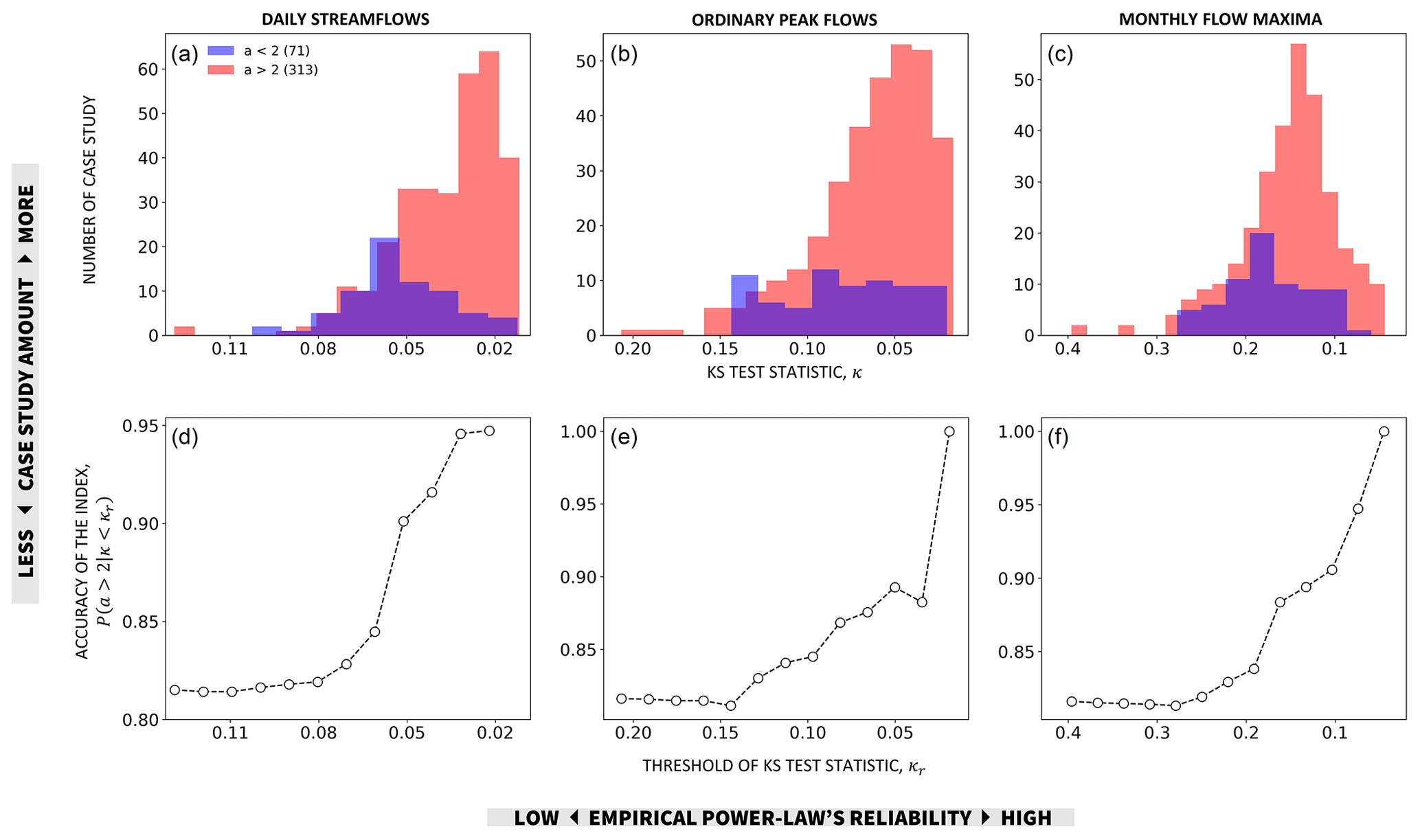
Figure 1 Accuracy of the proposed index. (a–c) Number of analyzed case studies as a function of the KS statistic κ of empirically fitted power-law distributions (the latter is a measure of how reliable the power law is as a model for the given data: the lower κ, the more reliable the power-law model). Case studies are identified as having either heavy- (a>2, red histograms) or non-heavy-tailed (a<2, green histograms) behavior based on the hydrograph recession exponent a estimated from daily flow records, which is proposed as an index of heavy-tailed streamflow and flood behavior. (d–f) Accuracy of the proposed index as a function of decreasing thresholds of κ_r (i.e., increasing reliability of empirical power laws). The values of the KS statistic κ are derived from records of (a, d) daily streamflows, (b, e) ordinary peak flows, and (c, f) monthly flow maxima.

We further estimate the accuracy of the proposed index based on the fraction of case studies that are identified as heavy tailed by the proposed index among all cases that are heavy tailed according to the available observations. To define the latter, we set a threshold value of κ: the power law is a reliable representation of the data for cases with κ below the threshold. Mathematically, the accuracy can be expressed as $P(a>\mathrm{2}\mathrm{|}\mathit{\kappa }<{\mathit{\kappa }}_{\mathrm{r}})=N_{\mathrm{c}}(a>\mathrm{2}\mathrm{|}\mathit{\kappa }<{\mathit{\kappa }}_{\mathrm{r}})/N_{\mathrm{c}}(\mathit{\kappa }<{\mathit{\kappa }}_{\mathrm{r}})$, where κ_r is the imposed threshold of κ, N_c(κ<κ_r) is the number of case studies whose κ<κ_r, and $N_{\mathrm{c}}(a>\mathrm{2}\mathrm{|}\mathit{\kappa }<{\mathit{\kappa }}_{\mathrm{r}})$ is the number of case studies with a>2 among the N_c(κ<κ_r) case studies. Higher accuracy essentially means that a higher fraction of heavy-tailed cases is correctly identified by means of the proposed index. To achieve this, we systematically reduce the threshold of the KS statistic κ_r (imposing a more stringent criterion for incorporating cases in the computation of the conditional probability of accuracy) along the x axis in Fig. 1, progressing from left to right. It is important to note that, as the κ_r threshold becomes smaller, the reliability of describing the data using power-law distributions increases (as denoted by the second axis legend of Fig. 1).

Figure 1d—f display the accuracy of the proposed index as a function of the reliability threshold κ_r. In all three cases (daily streamflows, ordinary peak flows, and monthly flow maxima), the accuracy values increase with the reliability level of the power-law distribution fitted on observed data. This means that the proposed index shows high accuracy for case studies where the empirical distributions of observed data are more consistent with power laws. In other words, the proposed index, which is estimated from common streamflow dynamics as the hydrograph recession exponent, accurately identifies heavy-tailed behavior of streamflow and flood distributions displayed by the available observations.

We further employ the goodness-of-fit testing procedure proposed by Clauset et al. (2009) (Appendix A) to identify case studies for which the representation of daily streamflow, ordinary peak flows, and monthly maxima by means of power-law distributions is convincingly supported by the available data. We refer to these case studies as confirmed heavy-tailed cases (Fig. 2, black dots). Conversely, we term the remaining ones as uncertain cases (Fig. 2, gray). The latter label denotes the fact that it cannot be determined with certainty whether the distributions underlying the available observations in these cases are or are not power laws due to scarcity of data.

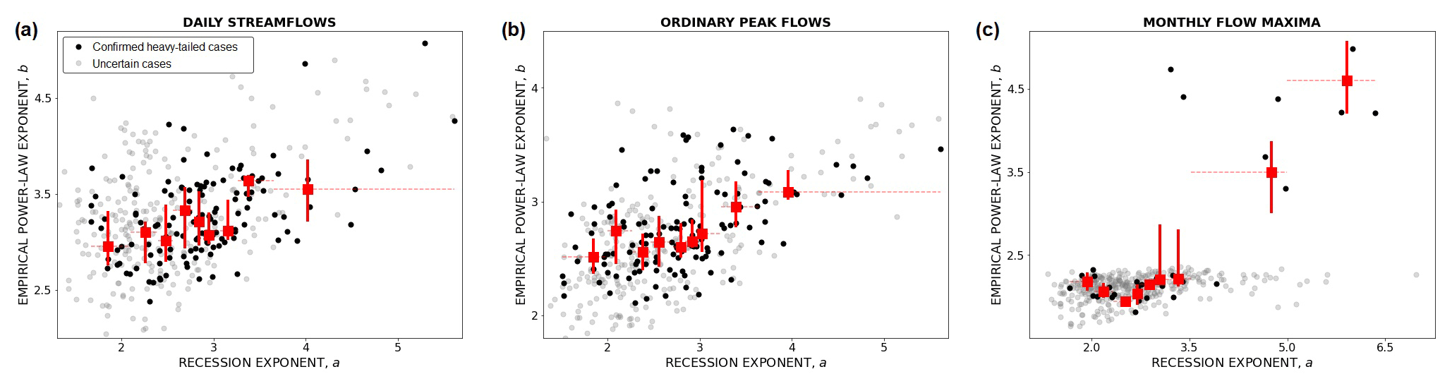
Figure 2 Empirical power-law exponent b as a function of the proposed index of heavy-tailed behavior a. Case studies are classified into groups of confirmed heavy-tailed (black dots) and uncertain (gray dots) cases on the basis of the hypothesis test (Appendix A; Clauset et al., 2009). The former denotes cases for which a power law provides a reliable description of the empirical data distribution, while the latter denotes cases whose data cannot convincingly support such a distribution. Red markers highlight the correlation between the empirical power-law exponent b and the hydrograph recession exponent a for confirmed heavy-tailed cases in the case of (a) daily streamflows (n=121 case studies), (b) ordinary peak flows (n=116), and (c) monthly flow maxima (n=34). Red markers display the median values of a and b (squares), the interquartile intervals of b (vertical bars), and the binning ranges of a (horizontal bars, equal number of case studies in each bin).

Figure 2 shows the empirical power-law exponent b as a function of the proposed index of heavy-tailed behavior a. Red markers display the median values of a and b (squares), the interquartile intervals of b (vertical bars), and the binning ranges of a (horizontal bars, equal number of case studies in each bin), highlighting the correlation between the empirical power-law exponent b and the hydrograph recession exponent a for confirmed heavy-tailed cases (black dots) in all three cases (i.e., daily streamflows, ordinary peak flows, and monthly flow maxima). We test the correlation by calculating their distance (Székely et al., 2007) and Spearman (Spearman, 1904) correlations, which are valid for both linear and nonlinear associations between random variables. We find that a and b are significantly correlated at a significance level of 0.05 in all three cases with distance (Spearman) correlation coefficients of 0.45, 0.44, and 0.81 (0.42, 0.46, and 0.60) for daily streamflows, ordinary peak flows, and monthly flow maxima. The high values of the correlation coefficients for monthly flow maxima are likely affected by the existence of two clusters in Fig. 2c. Nonetheless, the existence of a statistically significant correlation between the empirical power-law exponent and the proposed index, obtained for Fig. 2a–c, confirms that the proposed index can be used not only to identify heavy-tailed flood behavior (as Fig. 1 shows) but also to evaluate the degree of the tail heaviness of the underlying distributions.

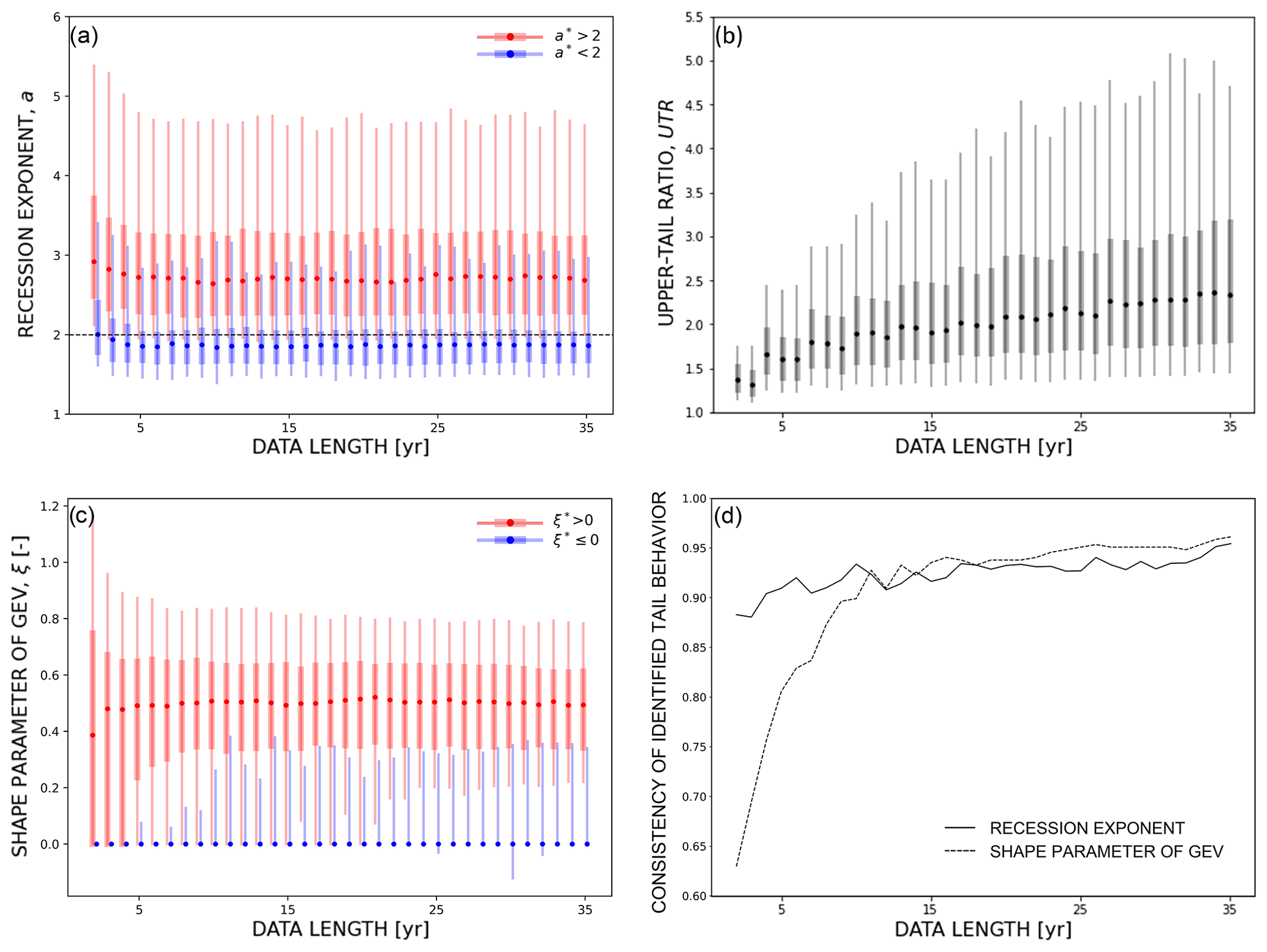
Figure 3 Stability of the categorization of case studies into heavy- and non-heavy-tailed flood behavior for decreasing data lengths. Estimates of three different indices of tail behavior as a function of data length. (a) Hydrograph recession exponent a (i.e., the proposed index of this study). Two frequently used metrics of heavy tails in hydrological studies: (b) the upper-tail ratio UTR and (c) the shape parameter ξ of the GEV distribution. Dots display the median values of the estimates for 386 case studies; vertical shaded bars and lines show the 0.25–0.75 and 0.05–0.95 quantile ranges of the estimates, respectively. The entire data record was used for computing the reference values of the hydrograph recession exponent a^* and the GEV shape parameter ξ^* and for categorizing each case study as either having (red) or not having (green) heavy-tailed behavior. (d) Consistency of identified tail behavior (either heavy or non-heavy) as a function of available data length for the indices recession exponent and shape parameter of GEV.

Figure 2c is of particular interest because it shows an example of the typical limitations of methods that rely solely on observations to determine the tail behavior of the distribution of maxima (e.g., Papalexiou and Koutsoyiannis, 2013), and, at the same time, it highlights the power of the proposed index. Large values of the recession exponent a, in agreement with corresponding large values of b, are found for all confirmed heavy-tailed cases (black dots in Fig. 2c) where the power law provides a plausible representation of the empirical distribution of monthly maxima. For uncertain cases (gray dots in Fig. 2c), the values of the empirical power-law exponents are unreliable (according to the applied method; Clauset et al., 2009) since it cannot be determined with certainty whether the empirical distributions are or are not power laws due to data scarcity. Conversely, the hydrograph recession exponent is calculated from daily streamflow data. We can therefore identify cases with heavy-tailed behavior and evaluate their tail heaviness based on the values of a. This estimate is deemed to be robust, provided that the predictions of the proposed index are confirmed by observations in cases (Fig. 2a and b) where data size is not a limitation (i.e., for daily streamflow and ordinary peak flows).

In Fig. 3 we test the stability of the categorization of case studies into heavy- and non-heavy-tailed flood behavior as provided by the proposed index (i.e., the hydrograph recession exponent a) for decreasing data lengths. We compare results for the proposed index against two other frequently used metrics of heavy tails in hydrological studies: (1) the upper-tail ratio (UTR) (Lu et al., 2017; Smith et al., 2018; Villarini et al., 2011) and (2) the shape parameter ξ of the GEV (generalized extreme value) distribution (Morrison and Smith, 2002; Papalexiou et al., 2013; Villarini and Smith, 2010). The UTR is defined as the ratio of the flood of record to the 0.9 quantile of floods (Smith et al., 2018), here represented by monthly flow maxima, while ξ is estimated by fitting a GEV distribution to the sample of monthly maxima using the Python package OpenTURNS 1.16 (Baudin et al., 2017). For all three indices (a, UTR, and ξ), we estimate their values for data lengths decreasing from 35 (i.e., the shortest entire record length in the dataset) to 2 years. We acknowledge that estimating parameters of extreme value distributions from such short records is not recommended. However, the exercise highlights the perks of the proposed index that, as it will be shown, is also able to provide robust results when only short data series are available. For each case study, we obtain 30 samples with the assigned test length from the entire data series using resampling without substitution (to avoid the results with a strong dependency on the specific streamflow time series). For each test length, we calculate the median values of the indices estimated from these samples and plot them in Fig. 3 together with their variability across case studies (vertical shaded bars and lines in Fig. 3 show the 0.25–0.75 and 0.05–0.95 quantile ranges of the index estimates across case studies).

To evaluate the consistency of the categorization of tail behavior across different data lengths, we proceed as follows. For each case we first compute the hydrograph recession exponent and GEV shape parameter from the entire data record and denote them with an asterisk superscript (i.e., a^* or ξ^*). Heavy-tailed cases are defined as having $a^{*}>\mathrm{2}$ or ${\mathit{\xi }}^{*}>\mathrm{0}$ (Godrèche et al., 2015), while non-heavy-tailed cases have values below these thresholds. To visualize heavy-tailed and non-heavy-tailed behaviors, we mark them in Fig. 3 in red and green colors, respectively, based on the reference values obtained from the entire data record. We then recalculate the indices from shorter samples and evaluate whether their values are consistent with the above categorization. For the UTR, we cannot implement this approach because there is no specific threshold for the identification of heavy- and non-heavy tails. We therefore directly compare the stability of the UTR's values across data lengths (a larger value indicates a heavier tail).

The proposed index provides consistent categorization of heavy- and non-heavy-tailed flood behavior across varying data lengths (Fig. 3a). The index estimates remain above 2 for most heavy-tailed cases (red) and below 2 for most non-heavy-tailed cases (green) (as defined according to the reference value a^* computed using the entire data record) when the data length decreases. The index estimates demonstrate the consistency throughout the test data length, as evidenced by the narrow range of variation in the median values of the estimates. For heavy-tailed cases, the median values ranged from 2.64 to 2.92, while for non-heavy-tailed cases, they ranged from 1.84 to 2.0. Additionally, the coefficient of variation for the estimates remained relatively constant, ranging from 0.29 to 0.33 for both heavy- and non-heavy-tailed cases. This indicates that the variability of the results (vertical shaded bars and lines in Fig. 3) is mostly due to pooling together different case studies belonging to the same category (heavy or non-heavy tailed) and does not increase as a result of decreasing length of the available data.

In contrast, the upper-tail ratio shows pronounced instability for decreasing data lengths (Fig. 3b). The median value of the index estimates varies between 1.32 and 2.36, with a coefficient of variation ranging from 0.15 to 0.64. These values indicate uncertain assessments based on the UTR and its tendency to underestimate the tail heaviness as the data length decreases.

Figure 3c illustrates the categorization of tail behavior using GEV shape parameter estimates. The results indicate that ξ estimates are stable with longer data series, yet their variability increases – leading to both underestimation and overestimation of tail heaviness – when the data length is short. To ensure a stable categorization of flood tail behavior using this method, data series spanning more than 10 years (for seasonal analyses and monthly maxima, i.e., sample sizes of around 30 values) are needed, in line with the findings of previous studies (Cai and Hames, 2010; Németh et al., 2019). The median values of ξ range from 0.39 to 0.52 for heavy-tailed cases and remain at 0 for non-heavy-tailed cases. Furthermore, the coefficient of variation demonstrates relatively higher variation across different test data lengths, ranging from 0.37 to 1.03 for heavy-tailed cases.

Figure 3d presents a summary of the consistency in identifying tail behavior (either heavy or non-heavy) compared to the identification based on the complete data record (i.e., the y axis in Fig. 3d shows the fraction of cases for which categorization based on shorter data series provides the same result obtained with the complete data record). This assessment is conducted for both the methods of recession exponents and GEV shape parameters (unfortunately, this approach is inapplicable to the UTR due to the absence of a specific threshold for distinguishing heavy and non-heavy tails). For data series longer than 10 years, both indices (ξ and a) exhibit comparable consistency and display an ascending trend, with the performance of the GEV shape parameters being slightly higher than the one of the recession exponents. Conversely, when analyzing data series shorter than 10 years, the performance of the shape parameter of the GEV drops, whereas the consistency of the hydrograph recession exponent, although slightly declining, maintains high values.

This result is possible because the proposed index infers heavy-tailed behavior from common discharge dynamics through the analysis of hydrograph recessions instead of fitting probability distributions to short records of extreme values as conventional approaches do. This allows for a more effective use of information contained in the data. For example, in the 2-year sample, we analyze a median number of four hydrograph recessions (which is not a large number), but these recessions have an average length of 8 d, which is sufficient to robustly characterize typical discharge dynamics of the rivers (Biswal and Marani, 2010; Dralle et al., 2017). The literature also evidenced that the variability of the hydrograph recession exponent across events is limited (Biswal and Marani, 2010), which makes it possible to reliably characterize it from a few hydrograph recessions only.

5 Discussion

The assessment of flood tail behavior is challenging due to high levels of uncertainty arising from the limited lengths of records of floods, which are, by definition, rare events. This issue is particularly prominent when maxima are used in the analysis as in the annual-maximum approach. Despite the widespread use of this method, its limitations for what concerns the reliability of flood tail estimates are well recognized. Very large sample sizes are indeed essential for obtaining accurate predictions of tail behavior (Papalexiou and Koutsoyiannis, 2013).

To address the challenge of obtaining reliable estimates, alternative methods have been proposed. A frequently used approach is the peak-over-threshold analysis, which uses the information content of a larger sample of data (Lang et al., 1999; Pan et al., 2022). Previous studies have demonstrated that this method leads to lower uncertainty in estimating high floods (Kumar et al., 2020). Volpi et al. (2019) also showed the advantage of using all the available observations (i.e., not only the peaks over a certain threshold) for estimating extreme events. In summary, all these methods suggest that discharge values other than maxima can provide information about the characteristics of extreme events. Specifically, incorporating information from less extreme (but more numerous) observations can reduce the uncertainty in the estimation of extreme events and lead to improved accuracy. Furthermore, non-asymptotic methods suggest that extremes are realizations of the underlying ordinary events (Marani and Ignaccolo, 2015; Lombardo et al., 2019), which can thus be used to assess rare events. These methods have improved the estimation of extreme values, especially by reducing their uncertainty (Marra et al., 2018; Miniussi and Marani, 2020; Mushtaq et al., 2022; Hu et al., 2023).

Similarly to the latter approaches, the index introduced in this study (i.e., the hydrograph recession exponent) leverages information on ordinary discharge dynamics to infer the tail behavior of flood distributions. This approach entails some advantages: firstly, it extracts information from a larger amount of available streamflow data. Secondly, estimating the hydrograph recession exponent requires significantly less data than conventional approaches that involve fitting probability distributions to hydrological samples. But most importantly, the proposed index offers a mechanistic approach to understand the emergence of heavy-tailed flood behavior, thus providing a process-based alternative to methods that solely rely on statistical analysis of observations. We acknowledge that assumptions underlying the method (e.g., the description of daily rainfall as a Poisson process) may influence the identification of heavy-tailed behavior. However, the importance of understanding intrinsic watershed dynamics which promote the occurrence of extreme events and contributing factors that lead to heavy-tailed flood behavior (Tarasova et al., 2020; Mushtaq et al., 2023) was recently highlighted in a comprehensive review by Merz et al. (2022). Identifying reliable proxies for inferring such behavior (Wilson and Toumi, 2005) is also important. The proposed index, which represents such a proxy grounded in the intrinsic hydrologic dynamics of the river basin, is thus especially useful in the very common cases when the tail of the flood distribution cannot be known from limited available observations.

The hydrograph recession exponent (which is the identified index of heavy-tailed flood behavior) essentially represents the nonlinearity of the storage–discharge response in catchments (Wittenberg, 1999; Biswal and Marani, 2010). A higher degree of nonlinearity leads to higher peak flows and a heavier tail of the streamflow distribution (Basso et al., 2015). In agreement with these findings, former simulation-based and field studies have shown that high nonlinearity of the catchment hydrological response linked to an increase in the runoff-contributing area results in a marked increase in the slope of flood frequency curves (Fiorentino et al., 2007; Rogger et al., 2012), which may be indicative of a heavy-tailed flood behavior. Gioia et al. (2012) also demonstrated that a nonlinear catchment response can convert light-tailed rainfall inputs into flood distributions with heavy tails, further confirming the role of nonlinear storage–discharge responses in producing heavy-tailed flood behavior. Merz et al. (2022) established, based on a comprehensive review, that the nonlinearity of the catchment response is a plausible contributor to the emergence of heavy-tailed flood behavior. Additionally, Basso et al. (2023) demonstrated that the hydrograph recession exponent aids in predicting the propensity of rivers for generating extreme floods. In line with these studies, our research further highlights that the hydrograph recession exponent, which provides a description of catchment nonlinearity obtained from common streamflow dynamics, is capable of robustly identifying heavy-tailed flood behavior.

The findings in Fig. 2 showcase the drawbacks of relying on purely statistical data analyses (which supply the empirical power-law exponents b) to identify flood tail behavior and the advantages of adopting the mechanistic approach proposed in this study (which yields the hydrograph recession exponent a). The gray markers in Fig. 2 indicate uncertainty in determining whether the distribution has a power-law tail, which is shown to be more prevalent when the sample size is reduced based on statistical analyses according to the Clauset et al. (2009) method (in 69 % and 70 % of the case studies of daily streamflow and ordinary peak analyses, we do not know whether or not they exhibit heavy-tailed behavior. However, this percentage increases to 91 % in the analysis of monthly maxima). The proposed index finds a solution to these limitations through a mathematical description of hydrological processes. Such an index is shown to perform well in cases where statistical methods may be limited due to a lack of data, as confirmed by the significant correlations between the recession exponent and the reliably empirical power-law exponent in all three panels (represented by black dots in Fig. 2). Even in cases where the statistical method is unable to confirm the underlying distribution (e.g., monthly maxima in Fig. 2c), our proposed index can still provide robust estimates of tail heaviness based on the values of recession exponents. This is supported by the analyses of daily streamflows and ordinary peaks, where sample size is not a limitation and where the predictions of the proposed index are confirmed by observations. Overall, the proposed index offers a promising solution for accurately characterizing the tail behavior of flood distributions, especially when traditional statistical methods may be limited due to a lack of data.

Data scarcity is a major challenge for reliable flood hazard assessment, mainly because of relatively short hydrological data records worldwide (Lins, 2008). The availability of a robust index of heavy-tailed flood behavior that works even with short data records is desirable. We test three indices, namely the recession exponent (the proposed index), the upper-tail ratio (UTR), and the shape parameter of the generalized extreme value (GEV) distribution (ξ), for categorizing tail behavior for decreasing data lengths. The results (Fig. 3a) show that the recession exponent provides stable estimates and categorizes cases consistently into heavy or non-heavy tails for decreasing data lengths. Furthermore, the slight variation in the estimates of the recession exponent for each test data length implies that variation in estimates primarily arises from case study heterogeneity rather than decreasing data length. Conversely, UTR significantly underestimates both the tail heaviness and the variation across cases for decreasing data lengths (Fig. 3b). In agreement with previous studies, underestimation of tail heaviness occurred when using UTR when the sample size was small (Smith et al., 2018; Wietzke et al., 2020). Meanwhile, the categorization of tail behavior was stable for cases with datasets longer than 10 years using the GEV shape parameter. However, high uncertainty in the variation of estimates across cases is observed when available data are relatively short, as also highlighted by previous studies (e.g., Wietzke et al., 2020) (Fig. 3c). Implied by this observation is that the estimates are biased by the short analyzed data, and a longer data record is desirable for a more reliable fitting of a GEV to data (Papalexiou and Koutsoyiannis, 2013). In summary, both the recession exponent and the GEV shape parameter exhibit greater stability across data lengths than the UTR, which is highly dependent on the available amount of data. When comparing the first two indices (recession exponent and GEV shape parameter) (Fig. 3d), the recession exponent demonstrates a high level of stability across all data lengths, even those shorter than 10 years based on this study's analyses. On the other hand, the GEV shape parameter displays lower stability when the available data are shorter than 10 years, but this stability significantly improves as the data length exceeds 10 years. Beyond the 10-year threshold, both indices show comparable consistency and an upward trend, with GEV shape parameters slightly outperforming recession exponents.

The hydrograph recession exponent allows for at least two significant applications as a proxy for heavy-tailed flood behavior. Firstly, it can be directly used to improve comparability across catchments and to provide a fair assessment of mapping regional patterns of flood hazards (Merz et al., 2022). Traditionally, assessing flood behavior across catchments using the same record length has been preferred (Cunderlik and Burn, 2002), but this is often not possible due to differences in data availability. The proposed index can robustly estimate heavy-tailed flood behavior from data with different record lengths, overcoming this limitation. Secondly, it can be applied as a preliminary step to correctly identify whether a considered catchment exhibits heavy-tailed flood behavior or not and to select an appropriate probability distribution to be used in flood frequency analysis. This prior identification of tail behavior is crucial to avoid potential underestimation of flood extremes (Miniussi et al., 2020; Mushtaq et al., 2022).

6 Conclusions

A new index of heavy-tailed flood behavior is identified from a physically based description of streamflow dynamics. The new index is embodied by the hydrograph recession exponent and can be readily estimated from daily streamflow records. Our findings demonstrate that this index enables the identification of heavy- or non-heavy-tailed flood behaviors in a large set of case studies across Germany. Importantly, it provides an evaluation of the tail heaviness (i.e., the severity of flood risks) based on analyses of common discharge dynamics. The results also remain robust even with limited data records.

The proposed index addresses the main limitations of current approaches, including the lack of physical support and low reliability in cases with limited data records. By extracting more information from available data and manifesting the nonlinearity of the catchment response, it represents a reliable method for the selection of suitable underlying distributions for flood frequency analyses and for the assessment of the peril of extreme floods in data-poor areas.

Appendix A: Goodness-of-fit tests for the empirical power laws

To test if the empirical power law is a plausible underlying distribution of the observed data, we follow the hypothesis test proposed by Clauset et al. (2009). The null hypothesis is that the empirical power law is a plausible underlying distribution of the observed data. Residual errors exist between the empirical power law and the observed data, which can be estimated by the error distance ε_d by means of the Kolmogorov–Smirnov statistic. The Kolmogorov–Smirnov test is selected because it is one of the most common measures for non-normal data. The core of the hypothesis test is to statistically prove that the errors between the data and the power law (i.e., ε_d) are a rational fluctuation of sampling randomness rather than being drawn from an incorrect underlying distribution. To determine the rationality of the sampling randomness, a Monte Carlo procedure is introduced: (1) a large number of groups n of synthetic data (with the same size as the observed data) are randomly generated from the empirical power law; (2) the error distance ${\mathit{\epsilon }}_{{\mathrm{s}}_i}$ of each synthetic group to the empirical power law is calculated for i=1, 2, …, n; (3) the frequency of ε_s>ε_d defines the p value of the hypothesis test, which indicates the probability that the residual errors between the empirical power law and the observed data are located within the range of sampling randomness fluctuations; and (4) the rationality is determined by p>0.1 using this package.

When p≤0.1, the null hypothesis is rejected; that is, the observed data are not plausibly drawn from the empirical power law. On the contrary, the empirical power law is considered to be a plausible distribution for the observed data because their residual errors are a statistically rational fluctuation of sampling randomness when p>0.1. Notice that a greater p value is better in this case because the aim is to verify the null hypothesis rather than to indicate that it is unlikely to be correct, as others often considered. Thus, p>0.1 is a more rigorous setting than p>0.05 in this case.

The setting of n=1000 is used as an adequate (great enough) number of iterations in this framework to distinguish underlying distributions that are commonly mixed (as suggested by Clauset et al., 2009).

The hypothesis test of the empirical power law, including all the above procedures, can be implemented via the function test_pl in the Python package plfit 1.0.3 (https://pypi.org/project/plfit/, last access: 13 March 2023).

It is worth mentioning that, statistically, we cannot say that those who do not pass the hypothesis test are not power law distributions. There are at least two potential reasons for this result: (1) they are indeed not power law functions, or (2) conclusions about the underlying distribution cannot be drawn due to the high uncertainty in the empirical data with small sample sizes. We thus use the term uncertain cases to indicate this awareness in the main paper.

Appendix B: A reference map of gauges across Germany used in this study

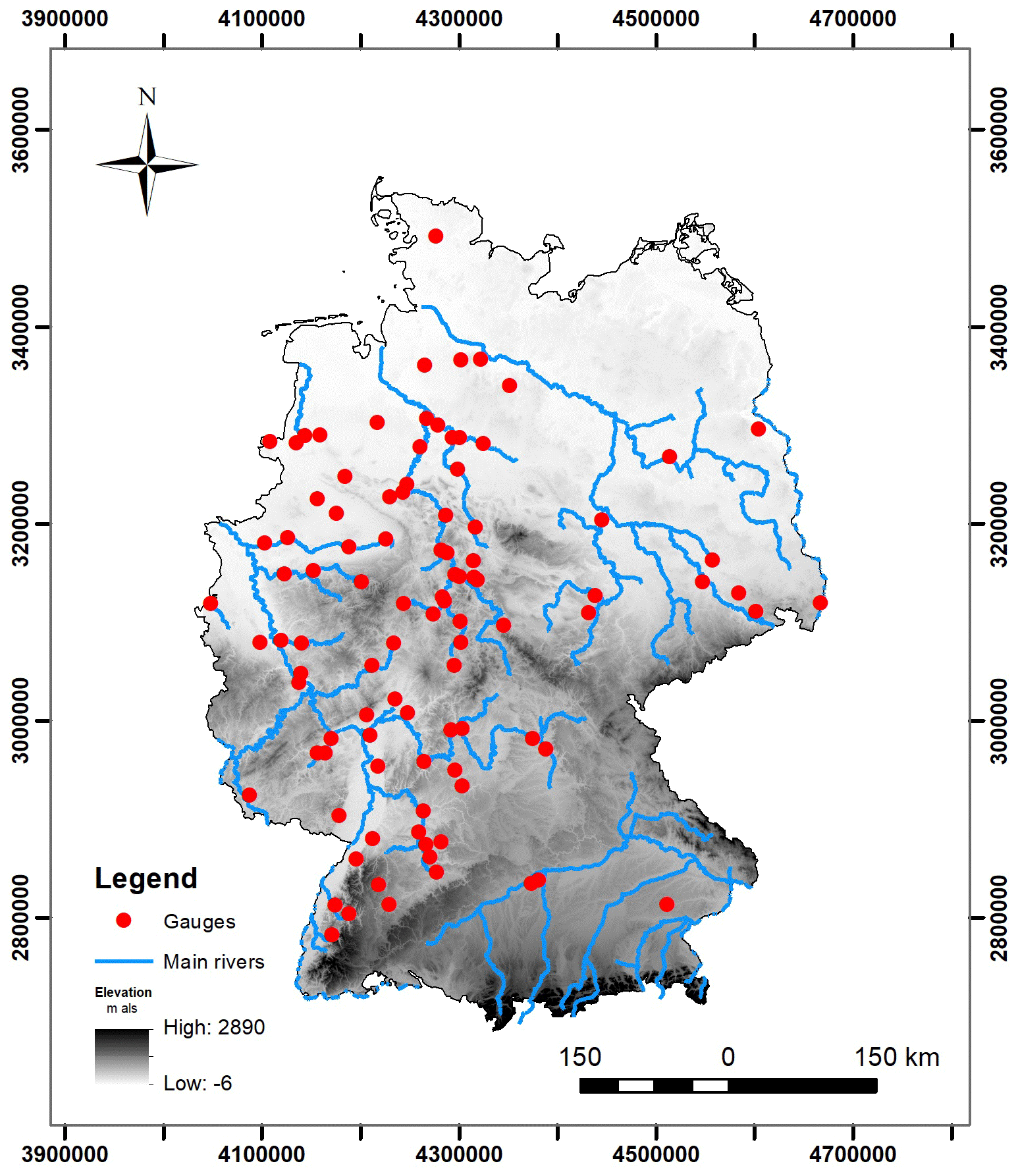
Figure B1 A reference map of gauges across Germany used in this study. These river basins encompass a variety of climate and physiographic settings without strong impact from dams and snowfall. Their areas range from 110 to 23 843 km² with a median value of 1195 km². The minimum, median, and maximum lengths of the daily streamflow records are 35, 58, and 63 years (in between 1951–2013).