Understanding the influence of “hot” models in climate impact studies: a hydrological perspective

Efficient adaptation strategies to climate change require the estimation of future impacts and the uncertainty surrounding this estimation. Over- or underestimating future uncertainty may lead to maladaptation. Hydrological impact studies typically use a top-down approach in which multiple climate models are used to assess the uncertainty related to the climate model structure and climate sensitivity. Despite ongoing debate, impact modelers have typically embraced the concept of “model democracy”, in which each climate model is considered equally fit. The newer Coupled Model Intercomparison Project Phase 6 (CMIP6) simulations, with several models showing a climate sensitivity larger than that of Phase 5 (CMIP5) and larger than the likely range based on past climate information and understanding of planetary physics, have reignited the model democracy debate. Some have suggested that “hot” models be removed from impact studies to avoid skewing impact results toward unlikely futures. Indeed, the inclusion of these models in impact studies carries a significant risk of overestimating the impact of climate change.

This large-sample study looks at the impact of removing hot models on the projections of future streamflow over 3107 North American catchments. More precisely, the variability in future projections of mean, high, and low flows is evaluated using an ensemble of 19 CMIP6 general circulation models (GCMs), 5 of which are deemed hot based on their global equilibrium climate sensitivity (ECS). The results show that the reduced ensemble of 14 climate models provides streamflow projections with reduced future variability for Canada, Alaska, the Southeast US, and along the Pacific coast. Elsewhere, the reduced ensemble has either no impact or results in increased variability in future streamflow, indicating that global outlier climate models do not necessarily provide regional outlier projections of future impacts. These results emphasize the delicate nature of climate model selection, especially based on global fitness metrics that may not be appropriate for local and regional assessments.

1 Introduction

Understanding the impact of climate change on water resources and hydrology is crucial for developing effective strategies for mitigation and adaptation (Eyring et al., 2019; Miara et al., 2017). The output of hydrological (e.g., Karlsson et al., 2016), water quality (Prajapati et al., 2023), and sediment transport (Sabokruhie et al., 2021) impact assessment studies is dependent on the choice of the future climate change projections. Hydrologists primarily use climate projection outputs from general circulation models (GCMs; e.g., Tabari, 2020) to study these impacts. The Coupled Model Intercomparison Project (CMIP) provides standardized metadata from coordinated simulations by different climate modeling groups (Meehl et al., 2007). The more recent Phase 6, CMIP6 (Eyring et al., 2016), is gradually replacing the widely used Phase 5, CMIP5, from the last decade (Hirabayashi et al., 2021; Martel et al., 2022; Zhang et al., 2023).

The concept of “model democracy” has been widely used in impact studies (e.g., Collins et al., 2013; IPCC, 2014), despite criticism (Knutti, 2010). This approach considers climate simulations to be independent and equally plausible, and it uses the ensemble mean and spread to define climate model uncertainty. Research has shown that the average of equally weighted projections outperforms single models with respect to simulating mean climatic patterns (Chen et al., 2017; Reichler and Kim, 2008). However, this approach may be less effective for the CMIP6 ensemble, as the validity of some simulations is under question (Hausfather et al., 2022).

The CMIP6 ensemble includes a subset of “hot” models that predict greater warming than previous predictions made by CMIP5 (e.g., Kreienkamp et al., 2020). These hot models have a climate sensitivity that exceeds the expected plausible range, which is based on observations and our understanding of planetary physics. They also exhibit a higher equilibrium climate sensitivity (ECS), a measure of the steady-state temperature increase in the event of doubled carbon dioxide (CO₂) concentrations in the atmosphere (Flynn and Mauritsen, 2020; Zelinka et al., 2020). The range of ECS values in CMIP6 models has increased to 1.8–5.6 ^∘C compared with 2.1–4.7 ^∘C in CMIP5, with an increase in the multi-model mean of 3.9 ^∘C in CMIP6 from 3.3 ^∘C in CMIP5 (Zelinka et al., 2020).

However, a plethora of evidence based on observations and our understanding of planetary physics indicates that we can confidently restrict the likely range of future warming trend and, more importantly, give less weight to extreme estimates (Liang et al., 2020; Tokarska et al., 2020). Recently, more research has been focused on constraining the ECS based on historical and paleoclimatic data (Knutti et al., 2017; Sherwood et al., 2020) or emergent constraints (Cox et al., 2018; Nijsse et al., 2020; Shiogama et al., 2022b). For example, Sherwood et al. (2020) used multiple lines of evidence and concluded that the likely (with a 66 % chance) ECS value is between 2.6 and 4.1 ^∘C. Consequently, the most recent reports published by the Intergovernmental Panel on Climate Change (IPCC) have narrowed the likely ECS range to 2.5–4 ^∘C (IPCC, 2023). It should be noted that the uncertainty surrounding the cooling impact (both direct and indirect) of aerosols on radiative forcing poses challenges in constraining future warming estimates (Bellouin et al., 2020; Forster et al., 2013; Smith et al., 2021). In essence, the current historical measurements do not provide a clear understanding of whether we are in a high-sensitivity, fast-warming scenario accompanied by strong contemporary aerosol cooling or if the situation is the opposite.

Climate change impact studies that include models with a high ECS may be biased and may overestimate the magnitude of impacts (Hausfather et al., 2022). Using the full ensemble of CMIP6 projections without restricting the hot models may no longer be the most appropriate option for impact studies (Ribes et al., 2021). Incorporating climate models with high sensitivity into impact studies may potentially lead to an overestimation of the overall economic consequences arising from future climate changes (Shiogama et al., 2022a). For instance, Shiogama et al. (2021) proposed a subset selection method that involved screening out hot models as the first step. On the other hand, Palmer et al. (2023) found that models with a higher sensitivity better represent some key climatic processes over Europe. While they were unable to provide robust physical explanations for their findings, it is worth noting that hot models may provide valuable information at the regional scale and that this information may be more important than the global warming trend for impact modelers, adding to the complexity of selecting models for regional impact studies.

The decision to weight climate models for impact studies remains controversial, but it is difficult to ignore the potential pitfalls of using hot models in these studies (Hausfather et al., 2022). This study aims to evaluate how including or excluding hot models in a multi-model ensemble affects the results of a large-scale hydrological climate change impact study. This influence is measured in terms of the magnitude and uncertainty in various streamflow metrics for 3107 North American catchments.

2 Materials and methods

The data for this study were obtained from the HYSETS database, which contains hydrometeorological data from various sources for over 14 000 catchments in North America (Arsenault et al., 2020b). The database includes all necessary data for the reference period of this study, including catchment boundaries (in the form of shapefiles), streamflow observations, weather observations (from stations as well as multiple gridded and reanalysis datasets), and static catchment descriptors (such as area, slope, elevation, land-use fractions, and soil properties). This study used the ERA5 reanalysis dataset, which was found to be a reliable alternative to gauge observations in a previous large-scale comparison study over the same study area (Tarek et al., 2020), for meteorological data. To ensure representativeness, a subset of HYSETS catchments were selected using filters. First, catchments with drainage areas below 500 km² were excluded, as daily hydrological models would be inappropriate for modeling hydrological processes at smaller scales. Next, catchments required at least 10 years of data to ensure sufficient data to successfully calibrate hydrological models and bias-correct climate models. Overall, 3107 catchments were retained.

Table 1 presents the list of 19 CMIP6 GCMs selected for this study. This list includes five hot models, defined by an ECS greater than 4.1. These models are as follows: CanESM5 (ECS of 5.62), NESM3 (ECS of 4.68), IPSL-CM6A-LR (ECS of 4.52), EC-Earth3-Veg (ECS of 4.3), and EC-Earth3 (ECS of 4.2). This study will be able to compare the uncertainty generated by the entire ensemble (19 models) to that of a reduced ensemble (14 models) obtained by removing the 5 hot models.

Table 1 The 19 GCMs selected in this study and their corresponding ECS values.

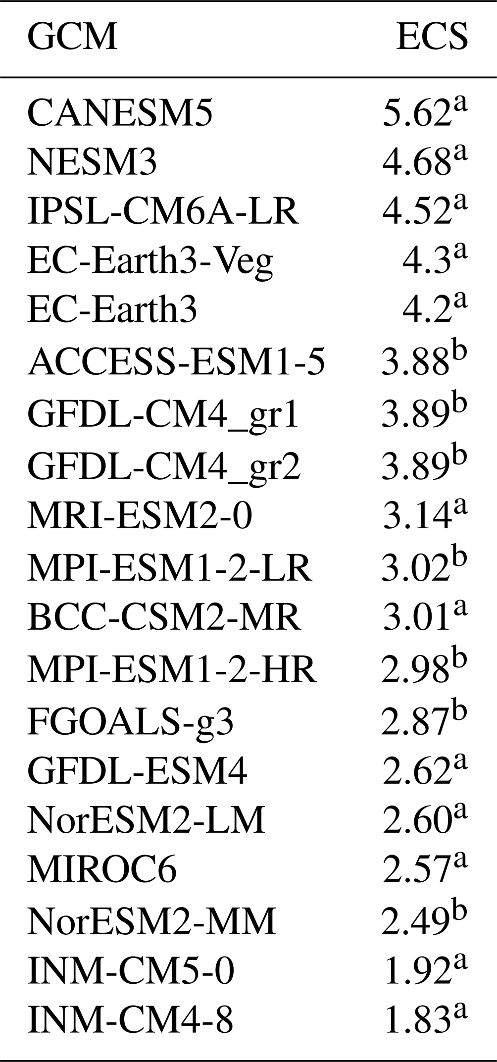
^a ECS values were taken from Tokarska et al. (2020). ^b ECS values were taken from Hausfather et al. (2022).

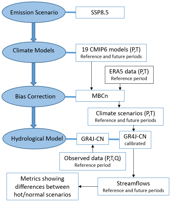
The impact study in this paper uses a traditional top-down hydroclimatic modeling chain consisting of one shared socioeconomic pathway (SSP8.5), 19 CMIP6 GCMs, one bias correction method, and one hydrological model. The study focuses solely on GCM uncertainty and does not consider other components, such as alternative SSPs, bias correction methods, or hydrological models, which would add uncertainty to future projections. These have been explored in previous studies (e.g., Wilby and Harris, 2006; Chen et al., 2011; Giuntoli et al., 2018; Troin et al., 2022) and are outside the scope of this work. The reference period is based on the 1971–2000 time frame, while the future climate is based on 2070–2099.

Figure 1 illustrates the methodological framework for each study catchment (Arsenault et al., 2020a). Precipitation and temperature data are first extracted from 19 CMIP6 climate models under the SSP8.5 scenario for both the reference and future periods. Using precipitation and temperature from the ERA5 reanalysis over the reference period, climate data are then bias-corrected using the multivariate bias correction (MBCn) method. These bias-corrected climate scenarios are subsequently employed as inputs for a calibrated hydrological model to compute streamflows. These computed streamflows are then employed to examine the impact of including (or not including) hot models in the impact study, using a set of defined metrics. Further details are provided below.

Figure 1 Methodological framework performed for each of the study catchments.

Climate models are mathematical representations of the Earth's climate system, based on current understanding of its physics and chemistry. They are formulated using simplifying assumptions and parameterizations but may not fully capture the complexity of the real climate system due to limited observations and understanding. As a result, climate models can be biased when compared with observations, due to factors such as model resolution, errors in reference datasets, and sensitivity to initial conditions. To ensure realistic impact simulations in impact studies, it is important to bias-correct climate model outputs. In this work, Cannon's (2018) N-dimensional MBCn method was used to correct biases in daily precipitation and temperature. MBCn is considered the most advanced and efficient quantile-based multivariate bias correction method, as reported by studies such as Chen et al. (2018), Su et al. (2020), and Cannon et al. (2020). MBCn transfers the distribution of observational data to the corresponding distribution from the climate model while preserving the projection trends of the climate model simulation crucial for climate change impact studies (Maraun, 2016). No downscaling was performed because this study was conducted at the catchment scale.

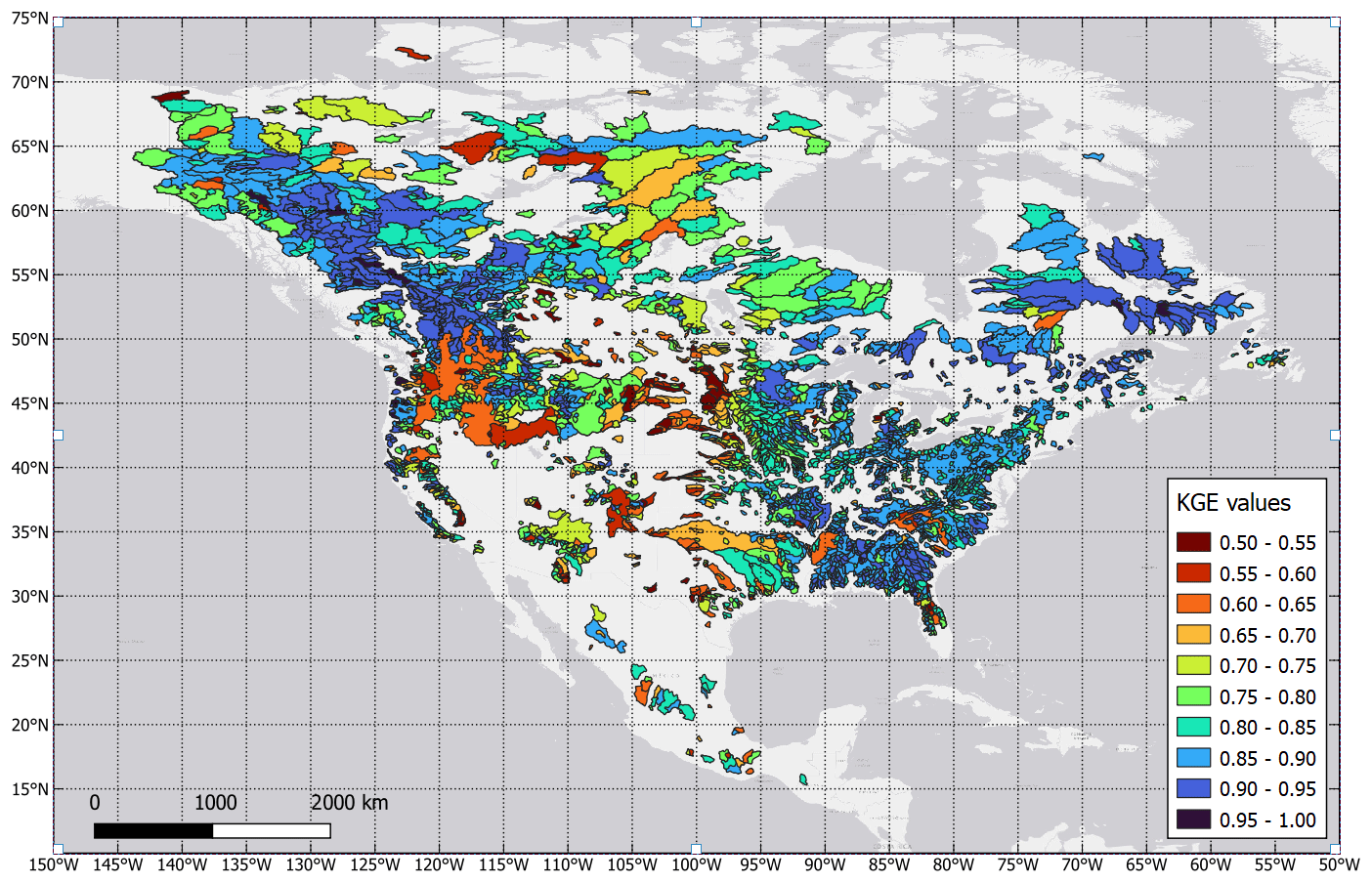
Figure 2 Study catchment location. The color scale corresponds to the hydrological model Kling–Gupta efficiency (KGE) calibration score over the reference period. Only catchments with available data, a KGE values higher than 0.5, and an area larger than 500 km² were selected.

In this study, the GR4J lumped rainfall–runoff model (Perrin et al., 2003) was chosen to simulate streamflows. The model was selected due to the large number of catchments, which made it infeasible to use more complex, distributed models. Additionally, lumped models use averaged temperature and precipitation at the catchment scale, which is more consistent with the scale of GCMs, eliminating the need for downscaling. Lumped models have been shown to perform well with respect to simulating streamflows at catchment outlets (e.g., dos Santos et al., 2018; Reed et al., 2004). The GR4J model is simple, efficient, and shows high performance compared with other lumped conceptual models. It uses precipitation, potential evapotranspiration (PET), and catchment surface area as inputs. To account for snow accumulation in some catchments, the GR4J model is linked with the CemaNeige snow module (Valéry et al., 2014), resulting in a six-parameter model (GR4J-CN). The GR4J-CN model combination has been used in many studies, including climate change impact studies, and has been shown to perform well under a wide range of conditions (e.g., Riboust et al., 2019; Tarek et al., 2020; Wang et al., 2019). The calibration was performed using the Kling–Gupta efficiency (KGE) metric. The KGE metric (Gupta et al., 2009) directly combines the bias, ratio of variance, and correlation into a single metric. It provides a more robust and refined assessment of model performance when calibrating hydrological models, addressing the drawbacks of the Nash–Sutcliffe efficiency (NSE) metric (Nash and Sutcliffe, 1970; Knoben et al., 2019). Figure 2 presents the location of the 3107 retained catchments, which all have a KGE calibration value above 0.5.

The hydroclimatic modeling chain described above generated 19 different 30-year time series of daily streamflow for the 2070–2099 future period, each corresponding to one of the 19 GCMs listed in Table 1. Three streamflow metrics were extracted from each 30-year time series, representing mass balance (Q_mean) and high (Q_max) and low (Q_min) flows:

• Q_mean was obtained by averaging daily streamflow over the 30-year period;

• Q_max was obtained by averaging the 30 annual maximum simulated streamflows;

• Q_min was obtained by averaging the 30 annual minimum simulated streamflows.

These metrics will be used to assess the impact of removing hot climate models across a range of flow conditions.

Figure 3 presents the three dispersion metrics used in this study to compare the spread (or uncertainty) of future projections of streamflow metrics. For the three streamflow metrics, 19 values from the original ensemble and 14 from the reduced ensemble for both the reference and future periods are extracted. The spread of the streamflow projections over the reference period is small, but it is not zero due to imperfect bias correction and the hydrology model's strong nonlinear response to precipitation and temperature inputs. The spread is comparatively much larger in the future period, mainly due to differences in the sensitivity and structure of the climate models.

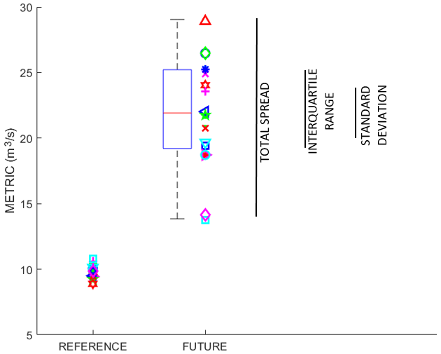
Figure 3 Representation of the dispersion metrics used in this paper. Each marker represents one of the 19 climate models. METRIC refers to Q_mean, Q_max, or Q_min, all in units of cubic meters per second (m³ s⁻¹).

Total spread (TS) is defined as the full range of future streamflow responses:

$$\begin{array}{}\text{(1)}& \mathrm{TS}={\mathrm{metric}}_{\max }-{\mathrm{metric}}_{\min }.\end{array}$$

The interquartile range (IQR) is defined as the distance between the 75th and 25th quantiles of the distribution, as shown by the blue rectangle in the box plot in Fig. 3.

$$\begin{array}{}\text{(2)}& \mathrm{IQR}=Q_{\mathrm{75}}-Q_{\mathrm{25}}\end{array}$$

Finally, the standard deviation (σ) is the standard mathematical measure of dispersion. In the case of a normal distribution, the standard deviation and interquartile range are perfectly correlated, but this may not be the case for a skewed distribution.

All three metrics have units of cubic meters per second (m³ s⁻¹) and are, therefore, dependent on catchment size and, to a lesser extent, mean annual precipitation. To account for this, the metrics will be presented in a nondimensional form:

$$\begin{array}{}\text{(3)}& {\mathrm{TS}}_{\mathrm{nd}}={\displaystyle \frac{{\mathrm{TS}}_{\mathrm{14}}}{{\mathrm{TS}}_{\mathrm{19}}}},\end{array}$$

where TS₁₉ and TS₁₄ represent the total spread for the full and reduced ensemble, respectively. TS_nd varies between 0 and 1: TS_nd=1 means that no reduction in total spread was obtained by removing the five warm models from the ensemble, whereas TS_nd=0 signifies that the total spread of the reduced ensemble has been totally eliminated.

Similarly, for the interquartile range ratio, we find the following:

$$\begin{array}{}\text{(4)}& {\mathrm{IQR}}_{\mathrm{nd}}={\displaystyle \frac{{\mathrm{IQR}}_{\mathrm{14}}}{{\mathrm{IQR}}_{\mathrm{19}}}}.\end{array}$$

However, in this case, the potential values vary in the 0–∞ range. More practically, a value below 1 indicates that the IQR has been reduced by removing the five hot models from the ensemble, whereas a value larger than 1 shows the opposite. The latter is possible if the removed models are somewhat close to the median of the ensemble.

Finally, for the standard deviation the following ratio is used:

$$\begin{array}{}\text{(5)}& {\mathit{\sigma }}_{\mathrm{nd}}={\displaystyle \frac{{\mathit{\sigma }}_{\mathrm{14}}}{{\mathit{\sigma }}_{\mathrm{19}}}},\end{array}$$

where a value below 1 indicates a smaller standard deviation for the reduced ensemble, and the opposite for a value above 1. σ_nd has the same possible range of values as IQR_nd (0–∞).

3 Results

Figure 4a presents the box plots of projected temperature increases for each of the 3107 catchments and for each climate model. The box plots provide a visual representation of key elements of the temperature increase distribution. The median of the distribution is shown as the red line near the center of the blue rectangle, which delimits the interquartile range (Q₇₅ and Q₂₅ for the upper and lower ends of the rectangle, respectively). The whiskers represent the 2.5th and 97.5th quantiles of the distribution, providing a 95 % coverage of the dataset. Quantiles below 2.5 and above 97.5 are shown as dots. Results indicate that the distribution of the projected temperature increases generally follows the same order as the ECS values presented in Table 1. However, there are some differences, which are not unexpected as global-scale ECS values are compared to regional-scale ΔT values. The five hot models are ranked as the first, second, third, fifth, and sixth hottest regional models based on median values (considering that GFDL-CM4_gr1 and GFDL-CM4_gr2 – fourth and fifth, respectively – are actually the same model with different spatial resolutions).

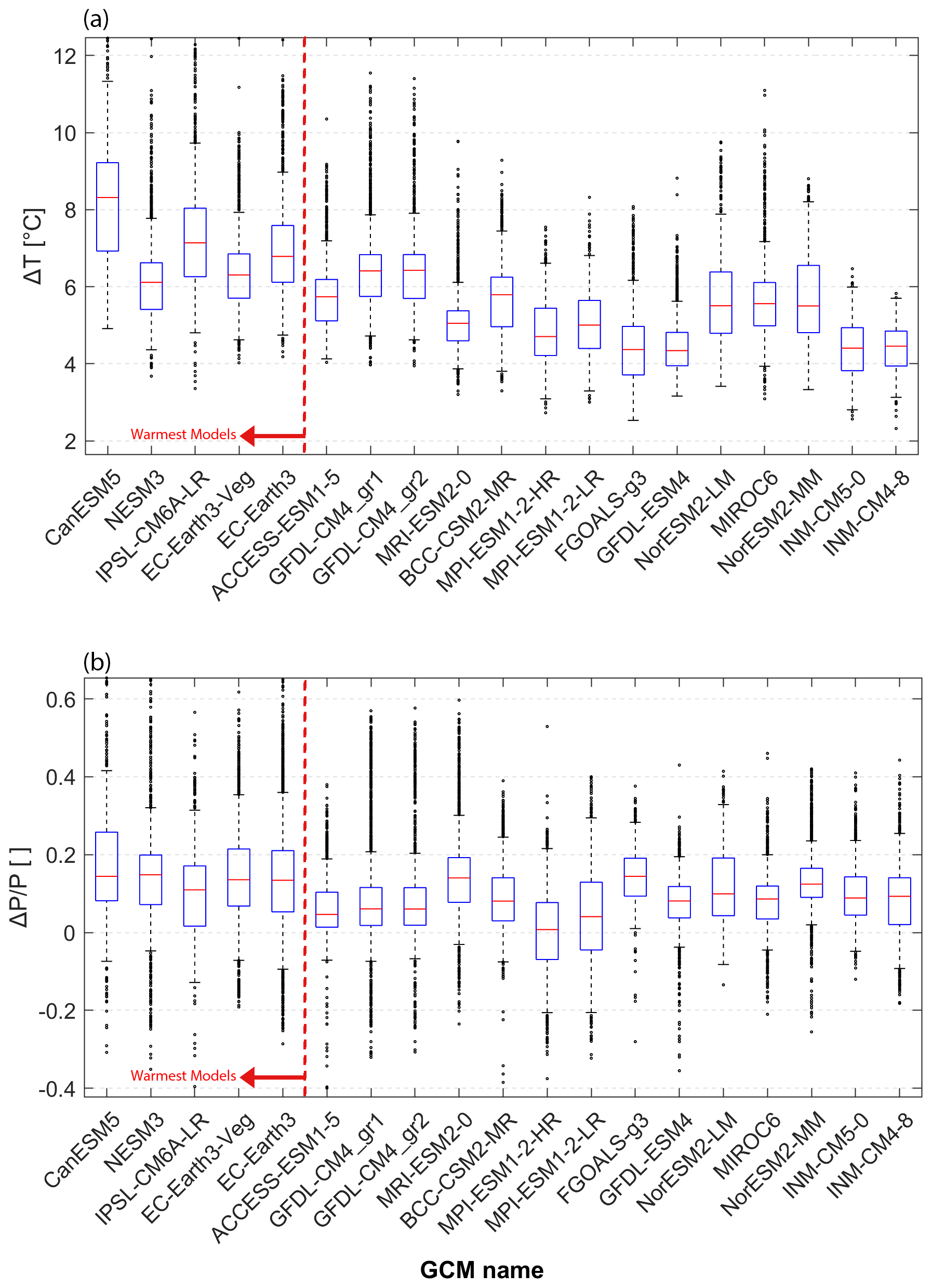
Figure 4 (a) Distribution of projected temperature increase (ΔT) and (b) projected relative annual precipitation increase ($\mathrm{\Delta }P/P$) for the 19 selected CMIP6 models for the 2070–2099 future period compared with the 1971–2000 reference period. Each box plot represents the distribution of the projected increases for the 3107 study catchments. The climate models are ordered in terms of their global-scale ECS values, starting with the largest on the left. The box plot whiskers correspond to the 2.5th and 97.5th quantiles, and a few catchment that were beyond the y axis limits are not shown.

Figure 4b presents the box plots of the projected changes in relative precipitation between the future and reference periods $\left(\frac{P_{\mathrm{fut}}-P_{\mathrm{ref}}}{P_{\mathrm{ref}}}\right)$. The box plots depict the distribution of the projected precipitation changes for each of the 3107 catchments. Results indicate that the hot models, identified by their ECS values, are also among the models with the largest projected changes in relative precipitation. Specifically, the five hot models are all within the group of the eight wettest models. The models with more modest increases in precipitation (e.g., MPI-ESM and ACCESS) are also among the cooler models. This trend is expected, as a warmer atmosphere can hold more moisture (up to 7 % ^∘C⁻¹, according to the Clausius–Clapeyron relationship), leading to more precipitation. Increased precipitation may mitigate the anticipated impacts of warmer models, such as increased evapotranspiration.

In order to show regional patterns related to Fig. 4, Fig. 5 displays the mean ΔT (Fig. 4a) and mean $\mathrm{\Delta }P/P$ (Fig. 4b) ratios between hot models and normal models. For temperature, a red color indicates that hot models are warmer than the other models on average. For precipitation, blue colors highlight increased precipitation in the hot models compared with the normal models. Overall, the hot global models exhibit a systematically larger temperature increase over the entire study domain. The hot models mostly exhibit increased precipitation compared with the normal models. However, the Pacific coast of the US as well as some catchments in the Southwestern US exhibit a decrease in precipitation according to the hot models. These observations underscore the regional variability in temperature and precipitation patterns when comparing hot and normal models.

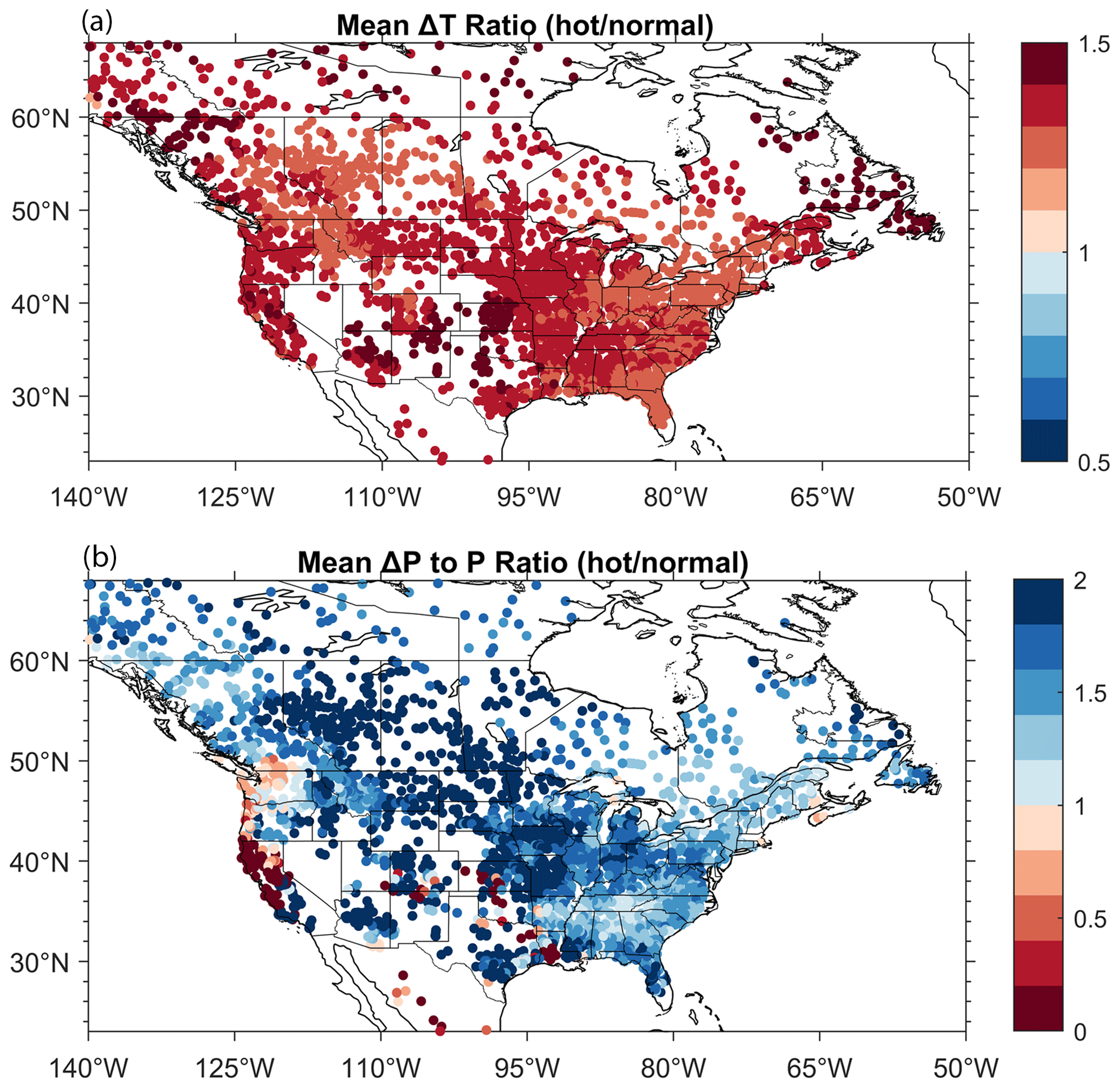
Figure 5 Mean ΔT (a) and $\mathrm{\Delta }P/P$ (b) ratios (hot models to normal models). For ΔT, a red color indicates that hot models are warmer, on average, than their normal (non-hot) counterparts. For $\mathrm{\Delta }P/P$, a blue color shows that hot models are wetter than their normal (non-hot) counterparts. The graphs represent the differences computed between the future and reference periods.

Figure 6 presents the ratio of mean projected streamflow changes (hot models / normal models) for Q_mean, Q_max, and Q_min. A blue color indicates larger projected streamflows by the hot models. Results show spatial patterns that differ depending on the streamflow metrics. Hot models project higher mean flows over most of the study domain, except in the southwestern regions, where increased evapotranspiration nullifies potential increases in precipitation. For Q_max, increases are mostly localized in the Eastern US, whereas Q_min values are widely increasing in Canada and mostly decreasing in the US.

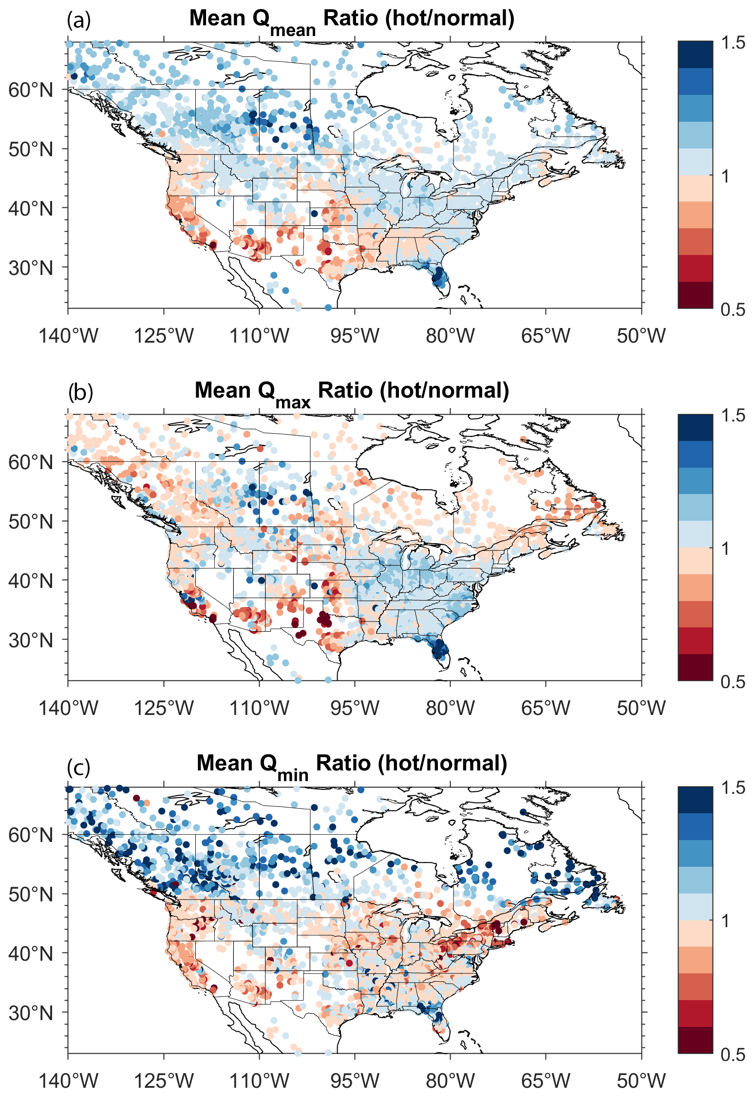
Figure 6 Ratio of mean projected changes (hot models divided by normal models) for (a) Q_mean, (b) Q_min, and (c) Q_max. A blue color shows that hot models project larger streamflows than their normal (non-hot) counterparts.

Figure 7 presents the TS_nd for mean (Q_mean), annual max (Q_max), and min (Q_min) streamflow obtained by removing the 5 hot models from the 19-member ensemble. A dark red color indicates no reduction in TS with the reduced ensemble, whereas lighter colors indicate a reduction. It can be seen that there is a clear spatial pattern that is relatively similar for all three streamflow metrics. The largest reductions in TS are seen in the northern regions as well as in the US Southeast, and along the US Pacific coast for Q_mean and Q_min. For all other regions of the US, no reduction in TS is observed. The reduced spread observed in the northern regions is smaller for Q_max. Despite these trends, a lot of variability remains present, with neighboring catchments sometimes showing contrasting behavior. More specifically, 57.0 % of the catchments see a decrease in TS for Q_mean, 53.3 % see a decrease for Q_max, and 61.7 % see a decrease for Q_min.

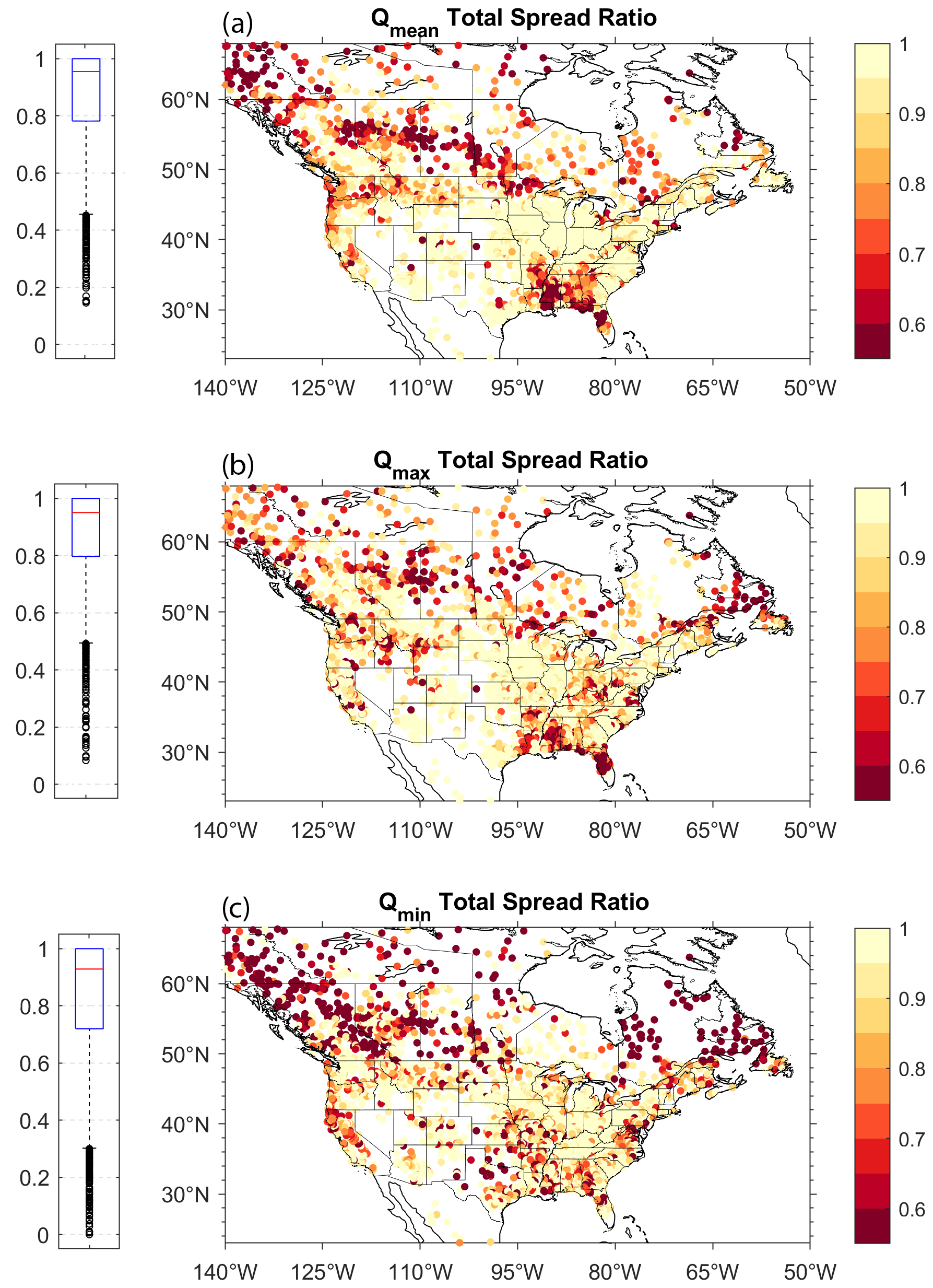
Figure 7 Total spread ratio $\left({\mathrm{TS}}_{\mathrm{nd}}=\frac{{\mathrm{TS}}_{\mathrm{14}}}{{\mathrm{TS}}_{\mathrm{19}}}\right)$ for Q_mean (a), Q_max (b), and Q_min (c) resulting from the removal of the five hot models. Box plots are shown on the left side of each panel.

The data from Fig. 7 are shown in the form of box plots on the left side of each panel to better illustrate the range of TS reduction. This shows that the median TS_nd is relatively high for all three streamflow metrics: 0.96 for Q_mean, 0.95 for Q_max, and 0.93 for Q_min. This is primarily because a significant number of catchments see no reduction in TS (43 %, 46.7 %, and 38.3 %, respectively). However, there is a significant reduction in TS observed in many catchments, and this decrease is strongly dependent on the geographical location of the catchments. Additionally, it can be seen that removing the hot models has a greater impact on Q_min than on the other two metrics.

The TS_nd is heavily impacted by outliers and may not accurately represent the overall spread of models. Figure 8 presents the σ_nd for the three streamflow metrics. A red color (σ_nd>1) indicates that the model spread has increased following the removal of the hot models, whereas a blue color (σ_nd<1) corresponds to a decrease. Results indicate that removing the hot models consistently reduces σ_nd in Canada for Q_mean and Q_min, as well as to a lesser extent for Q_max. However, for the continental US, the results are more complex, with a lot of regional variability. Removing outlier models in the North Central, Northeastern, and Southwestern US results in an increase in σ_nd for both Q_mean and Q_max. Overall, as shown in the box plots in Fig. 8, removing the hot models likely reduces the spread in roughly two-thirds of catchments, while one-third see an increase. These values are larger than those obtained for TS. The trends seen in the IQR_nd are also very similar to those of σ_nd (see Figs. S1 and S2 in the Supplement).

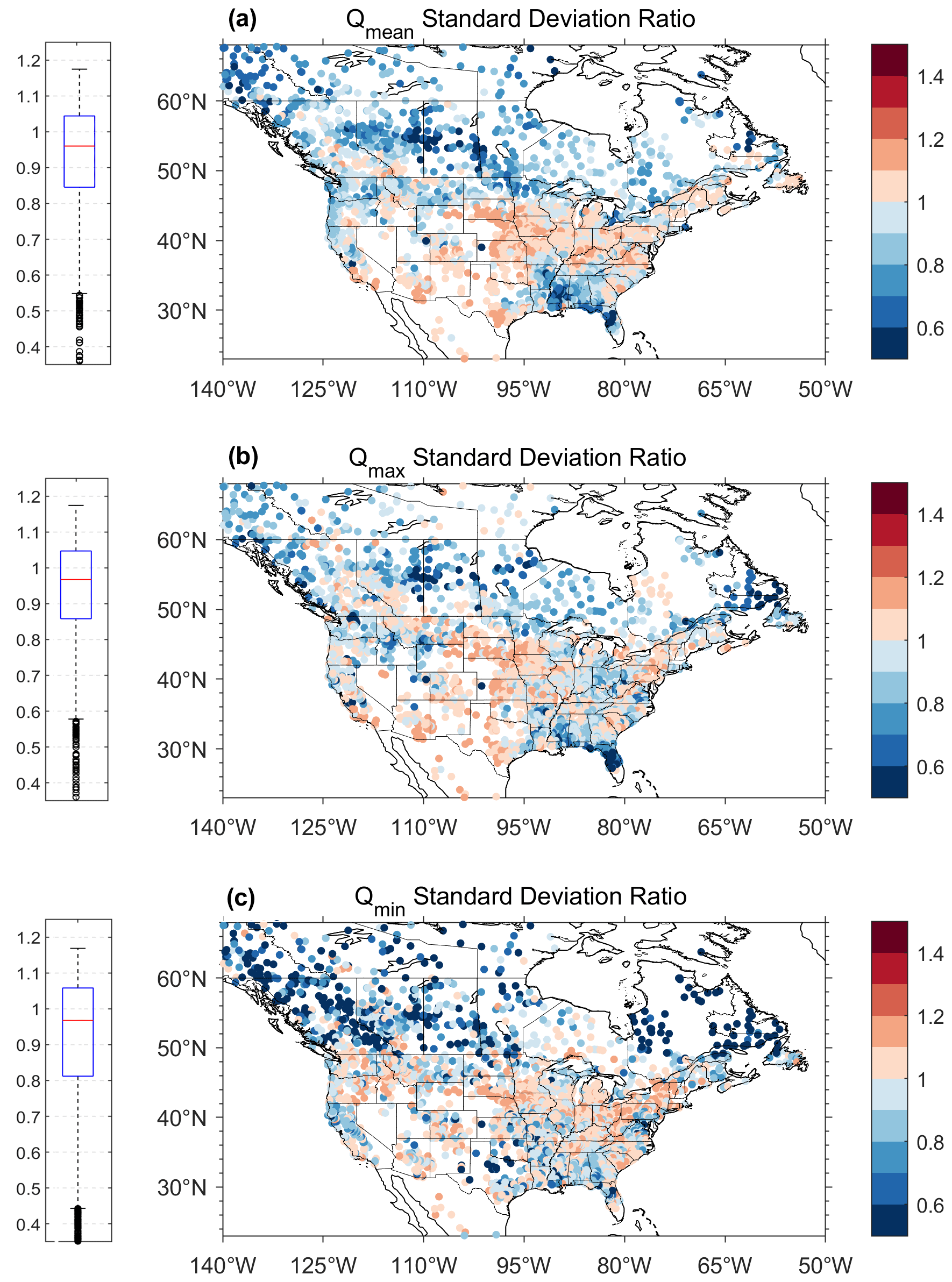
Figure 8 Standard deviation ratio $\left({\mathit{\sigma }}_{\mathrm{nd}}=\frac{{\mathit{\sigma }}_{\mathrm{14}}}{{\mathit{\sigma }}_{\mathrm{19}}}\right)$ for Q_mean (a), Q_max (b), and Q_min (c) resulting from the removal of the five hot models. Box plots are shown on the left side of each panel.

4 Discussion

Uncertainty is a key factor in assessing the impact of climate change. Different models and techniques, including various climate models, can lead to diverse climate projections and scenarios. Climate change interacts with other stressors, such as land-use change and population growth, in complex and unpredictable ways, making it important to accurately address uncertainty in climate impact studies to develop effective adaptation measures. Incorrectly representing uncertainty can lead to poor adaptation.

With the increased future temperatures, an intensification in the hydrological cycle is expected. However, this does not guarantee an automatic increase in water flow rates. This is because the rise in average temperature can also have a considerable impact on evapotranspiration. The outcome of these two factors working together is complex and varies based on the geographical location and primary climate zones. The research paper indicates that regions characterized as hot tend to be associated with increased precipitation, further complicating the relationship between temperature and water flow.

Results show that removing the hot models is likely to reduce the spread of three streamflow metrics. Between 60 % and 75 % of catchments show a decrease in the spread of future streamflow projections, indicating that the hot models are outliers or are further from the mean than the average model. In such cases, keeping the hot models would result in an overestimation of future streamflow uncertainty. However, removing the hot models also led to an increase in the spread in certain regions, indicating overconfidence in the results. This means that, although they are outliers with respect to the ECS, the hot models may not be outliers with respect to impact studies. Generally, a reduction in spread was evident in northern regions, such as Canada and Alaska, as well as the coast of California and the Southeastern region of the US. Shiogama et al. (2022b) also concluded that the inclusion of hot models leads to an overestimation of annual mean precipitation increases in Alaska, Canada, and the western US, where there is a substantial decrease in the variability in streamflow metrics.

A reduction in the spread of future streamflow is expected when removing the hot models or reducing the number of climate models. A bootstrapping methodology was used to determine if the changes in spread were due to a reduction in the number of models. This was conducted by selecting a random sample of 14 (out of 19) models 100 times and computing the average standard deviation ratio. This was repeated for all catchments, and the aggregated results are shown in Fig. 9.

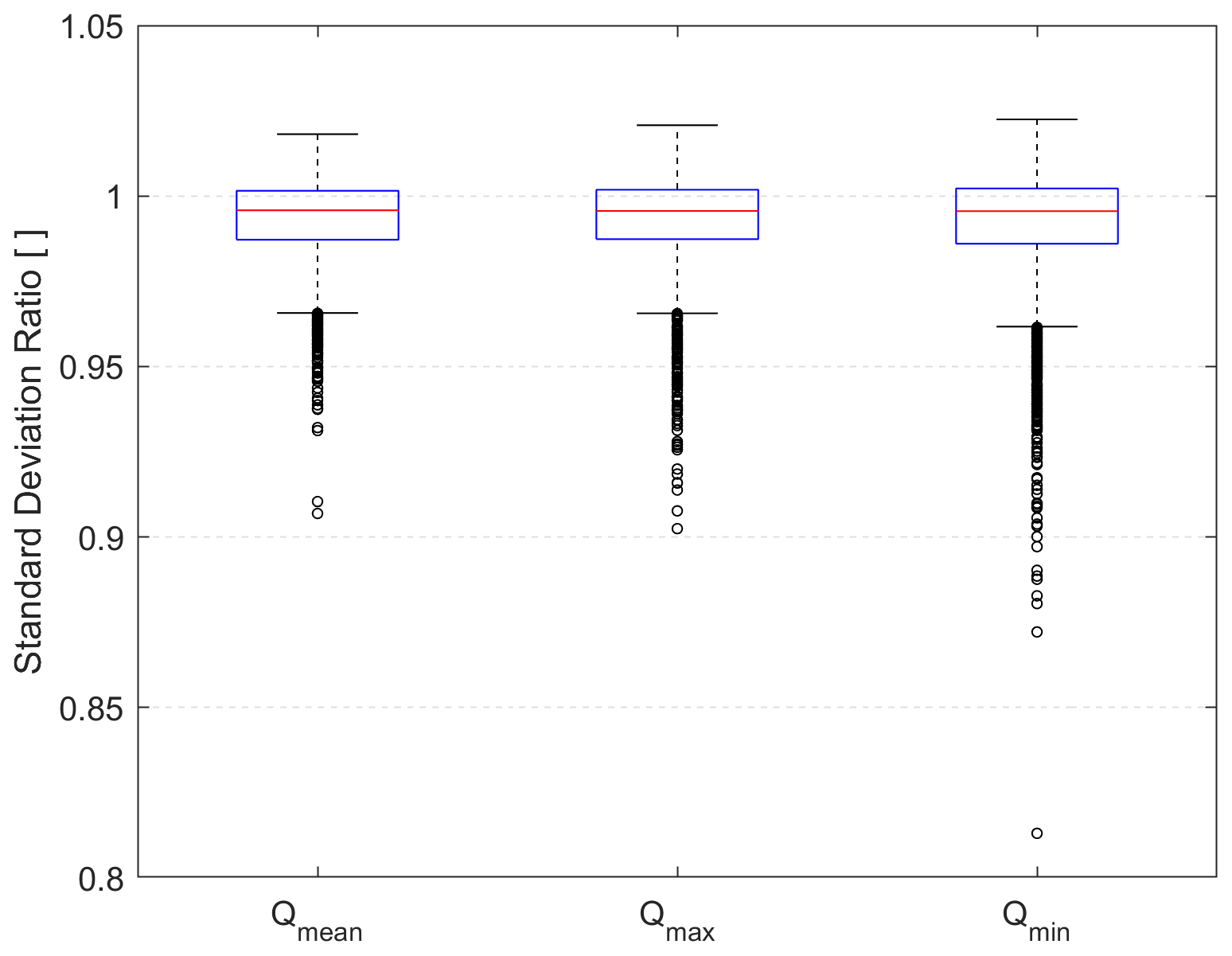
Figure 9 Box plots of the average standard deviation ratio for Q_mean, Q_max, and Q_min resulting from the removal of five random models, after sampling 100 random combinations of five models.

The results indicate that removing five random models results in a decrease in the standard deviation ratio almost 75 % of the time for all three streamflow metrics, but the median spread reduction ratio for this spread metric is extremely small (about 0.99 for all three streamflow metrics). This shows that removing the five hot models has a much larger impact than removing five random models. Therefore, the spread reduction observed in many catchments is not solely related to a reduction in the number of models.

At first glance, there is a strong physical reasoning for removing climate models with equilibrium climate sensitivity (ECS) values exceeding those expected from current data and the current understanding of planetary physics (Ribes et al., 2021; Shiogama et al., 2021). However, it should be noted that most impact studies are conducted at the regional or local scale, and these models may not be considered outliers at these scales. This study found that, although they may still be among the hottest in the study domain, globally hot models are not consistently the hottest, raising questions about whether their global behavior should automatically eliminate them from regional studies.

In this study, the climate performance of these models (such as their ability to represent climatic, hydroclimatic, or hydrological metrics) was not evaluated. The goal was to examine the impact of removing 5 hot models from a 19-member ensemble. However, it is important to note that judging climate models based solely on their ECS values may result in the removal of models that have desirable characteristics at the regional scale (e.g., Palmer et al., 2023). Additionally, keeping hot models may also be useful from an impact perspective because they may provide a clearer picture of future changes, as internal variability is less likely to obscure changes. This is similar to the rationale behind using high-emission scenarios in impact studies, such as SSP8.5, even though they may not be considered realistic scenarios anymore (e.g., Hausfather and Peters, 2020). It is important to consider worst-case scenarios when analyzing potential outcomes, as high levels of greenhouse gas emissions or high model sensitivity, such as those projected in SSP8.5 or high-ECS models, are not unrealistic, even though they may be less likely. While it is valuable to consider these high-end scenarios, it should be made clear that they are indeed worst-case scenarios.

In this study, the question of whether to remove the hot models for impact studies is complex. Results showed that removing these models increased the future uncertainty in streamflow for about one-third of all catchments. This suggests that these hot outliers may not always be hydrological outliers when put through a hydrological modeling process. Hydrological models are well known for being highly nonlinear integrators of weather variables, such as temperature and precipitation, and these results align with findings from other studies that have demonstrated the complex relationship between climate model projections and hydrological projections (e.g., Chen et al., 2016; Ross and Najjar, 2019). The fact that the CMIP6 hot climate models tend to be wet models may also be a factor in these results, as increased evapotranspiration could be offset by increased precipitation, leading to somewhat average results for the wrong reasons.

The regional impact of model importance is also compared (see Figs. S3 and S4, which demonstrate the total spread ratio resulting from removing a single climate model and creating an 18-member ensemble). Removing CanESM5 leads to a clear reduction in the total spread in Alaska and the Yukon (for Q_mean and Q_min) and in the Southeastern US for Q_max, indicating that CanESM5 is an outlier in these regions. Conversely, removing NESM3 does not result in significant decreases in spread over most of the study domain, as the high ECS value of NESM3 does not automatically translate into a correspondingly higher level of regional warming (see also Fig. 4), demonstrating that it is not an outlier in most regions. This underscores the strong regional differences among globally identified hot models.

The only uncertainty in this study is that originating from GCM/Earth system models. As stated earlier, in most impact studies, additional sources of uncertainty would also be incorporated. Additional greenhouse gas emission scenarios would be selected as well as other impact models (e.g., hydrology models). Downscaling and additional bias correction may be performed. These additional components are likely to generate additional uncertainty which may, in some cases, dwarf that of climate models. As such, many of the differences observed between the original and reduced climate model ensembles in this paper may have little impact on the final uncertainty estimation. For example, for low flows, many studies have shown that most of the uncertainty lies within the hydrology models (e.g., Giuntoli et al., 2018; Krysanova et al., 2018; Trudel et al., 2017) and that removing climate models would have no impact on uncertainty.

The results show that there is no simple answer as to whether or not including hot models in climate change impacts studies. In the absence of any computational limitations, we would recommend using as many climate models as possible and then subsequently studying the impact of including/excluding hot models. If the selection of a subset of climate models is necessary (e.g., inability to use a large ensemble due to limited computational capability or the cost of running impact models) removing hot models may be a reasonable option. Evaluating climate model fitness for impact studies is a difficult endeavor, and, in addition to the ECS, additional performance metrics should also carefully be taken into account.

5 Conclusion

This study examines the impact of removing a subset of hot climate models on the spread of future projections of streamflow for 3107 North American catchments. Three streamflow metrics were considered: mean annual streamflow and the means of the respective annual maximum and minimum streamflow, over the reference period (1971–2000) and future period (2070–2099).

Hot climate models are determined based on their global equilibrium climate sensitivity (ECS), whereas impact studies typically focus on the local to regional scale. The hot climate models remain among the hottest in our regional evaluation, but they also tend to be among the wettest, potentially leading to a complex hydrological response.

Our research revealed mixed impacts of removing the hot climate models. A decrease in the variability in the projected streamflow metrics was generally observed in Canada and Alaska, the Southeast US, and the Pacific coast of the US. However, in other regions, removing the hot models resulted in no changes or, in some cases, even increases in the variability in the projected flows. This suggests that the hot models are not necessarily hydrological outliers, raising questions about using global performance metrics rather than regional metrics for model selection.

The findings of this study emphasize the importance of carefully selecting climate models and the potential risks of including inadequate models in impact studies. In the absence of constraints, it is recommended to use as many climate models as possible when determining impact uncertainty and to assess the impact of subsets of climate models (based on high global equilibrium climate sensitivity or other performance metrics) a posteriori to evaluate the sensitivity of the impact model to climate model selection. These results highlight the need for further research on climate model fitness and the proper selection of model subsets for impact studies.