A statistical–dynamical approach for probabilistic prediction of sub-seasonal precipitation anomalies over 17 hydroclimatic regions in China

In this study, we develop a spatial–temporal projection-based calibration, bridging, and merging (STP-CBaM) method to improve probabilistic sub-seasonal precipitation forecast skill over 17 hydroclimatic regions in China. The calibration model is established by post-processing ECMWF raw forecasts using the Bayesian joint probability (BJP) approach. The bridging models are built using large-scale atmospheric intraseasonal predictors, including zonal wind at 200 hPa (U200) and 850 hPa (U850); an outgoing longwave radiation anomaly (OLRA); and geopotential height at 200 hPa (H200), 500 hPa (H500), and 850 hPa (H850) defined by the STP method. The calibration model and the bridging models are then merged through the Bayesian modelling averaging (BMA) method. Our results indicate that the forecast skill of the calibration model is higher compared to bridging models when the lead time is within 5–10 d. The U200- and OLRA-based bridging models outperform the calibration model in certain months and certain regions. The BMA-merged forecasts take advantage of both calibration models and bridging models. Meanwhile, the BMA-merged forecasts also show high reliability at longer lead times. However, some improvements to reliability are still needed at shorter lead times. These findings demonstrate the great potential to combine dynamical models and statistical models in improving sub-seasonal precipitation forecasts.

1 Introduction

Sub-seasonal forecasting (defined as the time range between 2 weeks and 2 months) bridges the gap between short- to medium-range weather forecasts and seasonal climate prediction (Vitart and Robertson, 2018; Liu et al., 2023). Skilful and reliable sub-seasonal precipitation forecasts are highly valuable for water resource management, flood disaster preparedness, and many other climate-sensitive sectors (White et al., 2022; Yan et al., 2023; Zhu et al., 2022). However, it is considered a difficult time range to generate skilful forecasts. The memory of atmospheric initial conditions is lost compared to short- to medium-range forecasts, while the variability of lower-boundary conditions, such as sea surface temperature, is too slow to take effect (Vitart and Robertson, 2018). Statistical models, which use observational relationships between sub-seasonal precipitation and atmospheric intraseasonal oscillations, have been developed in recent years. The spatial–temporal projection model (STPM), which extracts the coupled patterns of preceding atmospheric intraseasonal oscillations and precipitation, has shown skill in predicting sub-seasonal precipitation. Zhu and Li (2017) constructed STPMs over different climatic regions during the boreal summer monsoon season, and their results indicated that the STPMs could generate skilful forecasts for intraseasonal precipitation patterns with lead times of up to 20 d. Our previous study developed a spatial–temporal projection-based Bayesian hierarchical model (STP-BHM) to take the uncertainties in the relationships between atmospheric intraseasonal oscillations and sub-seasonal precipitation into account (Li et al., 2022). However, statistical models are highly reliant on stationary relationships between predictors and predictands. Seasonal changes in climatological conditions may lead to different relationships between atmospheric intraseasonal oscillations and precipitation. Liu and Lu (2022) suggested that the impacts of boreal summer intraseasonal oscillation (BSISO) on precipitation are different between early and late summers. W. Li et al. (2023) found that the long-period BSISO event-affected region and the associated precipitation anomalies are different compared to short-period BSISO events.

With a more comprehensive understanding and better representation of potential sources of predictability, there has been much improvement in dynamical models in recent years. The Subseasonal-to-Seasonal (S2S) prediction project and the Subseasonal Experiment (SubX) project have been established to provide S2S forecasts from dynamical models. However, the sub-seasonal precipitation forecasts of global climate models (GCMs) are always of low accuracy (de Andrade et al., 2019; Li et al., 2022). The physical equations are simplified, while the small-scale processes, such as convections, cannot be well represented in most GCMs. In addition, insufficient data assimilation schemes, low capacity in capturing dynamic sources, and misrepresentation of atmosphere–ocean interactions and atmosphere–ocean interactions also contribute to the limited forecast skill (Wu et al., 2023; Zhang et al., 2021). Although post-processing methods have been proposed in recent years, the forecast skill after post-processing was still limited for lead times beyond 10–14 d (Li et al., 2021).

Despite the low forecast skill of sub-seasonal precipitation, the GCMs show much higher performance in predicting large-scale circulation patterns. Cui et al. (2021) evaluated the potential of GCMs to predict intraseasonal surface air temperature over mid- to high-latitude Eurasia. Their results indicated that the upper limit of the useful forecast skill ranged from ∼10 to ∼20 d. The BSISO is the predominant variability of the Asian summer monsoon, and most GCMs exhibit predictability on timescales of above 3 weeks for BSISO events (Chen and Zhai, 2017; Hsu et al., 2016; Ren et al., 2018). Lee et al. (2015) evaluated the prediction skill of BSISO indices using six coupled models in the Intraseasonal Variability Hindcast Experiment (ISVHE) project, and their results suggested that skilful BSISO prediction was about 22 d under strong initial conditions. Shibuya et al. (2021) suggested that the overall useful prediction skill of the BSISO was approximately 24 d in a global non-hydrostatic icosahedral atmospheric model (NICAM) with explicit cloud microphysics. Similar results were also found by Wu et al. (2023), i.e. that the ECMWF model showed skilful prediction of the BSISO index at a 24 d lead time.

Given the strengths and weaknesses of both statistical models and dynamical models, there has been growing interest in developing hybrid prediction models that combine forecasts from both statistical and dynamical models (Slater et al., 2023). Schepen et al. (2014) used POAMA (Predictive Ocean Atmosphere Model for Australia) forecasts of seasonal climate indices as predictors to predict seasonal precipitation over Australia. Strazzo et al. (2019b) developed a hybrid statistical–dynamical system to predict seasonal temperature and precipitation over North America. Most previous statistical–dynamical models focus on seasonal predictions. Far fewer attempts have been made on sub-seasonal timescales. Specq and Batté (2020) proposed a statistical–dynamical post-processing scheme to improve the quality of sub-seasonal forecasts of weekly precipitation using Madden–Julian Oscillation (MJO) and El Niño–Southern Oscillation (ENSO) indices as predictors. Wu et al. (2022) established a dynamical–statistical prediction model (DSPM) to improve sub-seasonal precipitation forecasts. Deep-learning models were also proposed to predict sub-seasonal extreme rainfall events, with the GCM-predicted large-scale circulation patterns used as predictors (Xie et al., 2023). Zhu et al. (2023) developed a dynamical–statistical hybrid model using the novel indices of the zonal displacements of the South Asia high and the western Pacific sub-tropical high to predict the Meiyu intraseasonal variation. Nevertheless, the relationships between large-scale circulation patterns and sub-seasonal precipitation have high uncertainty. More sophisticated hybrid models are required to further improve the probabilistic sub-seasonal precipitation forecast skill.

The calibration, bridging, and merging (CBaM) method, which employed Bayesian-theorem-based approaches to take advantage of both dynamical models and statistical models, has proven able to generate skilful and reliable seasonal precipitation and temperature forecasts over different regions (Peng et al., 2014; Schepen et al., 2014, 2016; Strazzo et al., 2019a). In calibration, the Bayesian joint probability (BJP) approach was used to post-process raw precipitation forecasts derived from GCMs. The BJP approach was also used to generate probabilistic forecasts using large-scale circulation patterns as predictors. This was also referred to as bridging. The calibrated forecasts and bridged forecasts were then merged through the Bayesian modelling averaging (BMA) method (Wang et al., 2012). Most previous studies used the CBaM method to generate seasonal forecasts. However, much less work has been done on sub-seasonal timescales for several reasons. Compared to seasonal forecasts, there are far fewer climate indices that can be used as predictors on sub-seasonal timescales. Moreover, the atmospheric intraseasonal oscillations may have different effects on precipitation anomalies in different months. As a consequence, it is much more difficult to establish bridging models for sub-seasonal precipitation forecasts. In addition, the evolution of the intraseasonal variability of precipitation varies in different stages with different periods in different regions (Liu et al., 2020; Zhu and Li, 2017). The effectiveness of the calibration models will be greatly affected if seasonality is not considered.

In this study, we develop a spatial–temporal projection-based calibration, bridging, and merging (STP-CBaM) method to improve probabilistic sub-seasonal precipitation forecast skill by combining the strengths of both dynamical models and statistical models. The ECMWF sub-seasonal precipitation forecasts are calibrated using the BJP approach for each month. The bridging models are then built using large-scale atmospheric intraseasonal predictors defined by the STPM. The calibration model and bridging models are merged through the BMA method to generate skilful and reliable sub-seasonal precipitation forecasts. The STP-CBaM method will be applied to predict sub-seasonal precipitation anomalies over each hydroclimatic region during the boreal summer monsoon from May to October. The accuracy and reliability will be evaluated through a leave-one-year-out cross-validation strategy.

In the following two sections, the data and methodology are introduced. The prediction skill and reliability of the STP-CBaM method are provided in Sect. 4. Section 5 discusses the forecast skill, limitations, and future work. Key findings are summarized in Sect. 6.

2 Data

2.1 Precipitation dataset

In this study, China is divided into 17 hydroclimatic regions on the basis of both climate classifications and watershed division standards (Fig. 1). The precipitation data are derived from the latest Multi-Source Weighted-Ensemble Precipitation, version 2.8 (MSWEP V2.8) dataset. This dataset is developed by optimally merging precipitation data derived from gauge, satellite, and reanalysis datasets. It covers the period from 1979 to the near past with a spatial resolution of $\mathrm{0.1}{}^{\circ }\times \mathrm{0.1}{}^{\circ }$. Many studies have found that the MSWEP dataset is of a high quality over China (Y. Li et al., 2023; Liu et al., 2019; Guo et al., 2023).

Figure 1 The 17 hydroclimatic regions over China. Publisher's remark: please note that the above figure contains disputed territories.

2.2 Reanalysis dataset and outgoing long-wave radiation (OLR) dataset

The daily mean geopotential height at 200, 500, and 850 hPa (H200, H500, H850) and zonal wind at 200 hPa (U200) and 850 hPa (U850) are derived from the ERA5 (Hersbach et al., 2020) reanalysis dataset at https://cds.climate.copernicus.eu/ (last access: 10 December 2022). The daily mean OLR data are provided by the National Oceanic and Atmospheric Administration (NOAA) Physical Sciences Laboratory (PSL), Boulder, Colorado, USA, from their website at https://psl.noaa.gov (last access: 17 December 2022). The OLR data are developed from high-resolution infrared radiation sounder instruments and have been widely used over the globe. All daily mean data including U200, U850, OLR, H200, H500, and H850 are bilinearly interpolated onto a horizontal resolution of $\mathrm{2.5}{}^{\circ }\times \mathrm{2.5}{}^{\circ }$ over the period of 2001–2020.

2.3 Hindcast dataset

The ECMWF hindcast data of precipitation, U850, U200, OLR, H200, H500, and H850 are retrieved from the S2S database at http://apps.ecmwf.int/datasets/data/s2s/ (last access: 31 December 2022). Compared to other GCMs, the ECMWF model shows the highest forecast skill in various aspects (Jie et al., 2017; Wu et al., 2023; Zhang et al., 2021). In this study, we choose hindcasts when the ECMWF model version dates are in the year 2021 from May to October. Thus, the hindcasts cover the period of 2001–2020. The gridded precipitation hindcasts are area-weighted averages through 17 hydroclimatic regions as the observational data. In addition, all atmospheric hindcast fields including U200, U850, OLRA, H200, H500, and H850 are bilinearly interpolated onto a horizontal resolution of $\mathrm{2.5}{}^{\circ }\times \mathrm{2.5}{}^{\circ }$ as the reanalysis dataset.

3 Methodology

3.1 Intraseasonal signal extraction

In this study, a non-filtering method is used to extract 10–60 d signals for both atmospheric variables (U200, U850, OLRA, H200, H500, and H850) and precipitation (Hsu et al., 2015; Zhu et al., 2015). The climatological annual cycle of observational data is first removed by subtracting a 90 d low-pass filtered climatological component. Lower-frequency signals are then removed by subtracting the last 30 d running mean. The higher-frequency signals are then removed by taking a pentad mean. The variable derived in this way represents the observational 10–60 d signals of a daily atmospheric field or precipitation. The daily intraseasonal signals are then averaged to pentad data to further reduce the noise and improve the predictability. The pentad mean 10–60 d intraseasonal precipitation is also referred to as pentad mean precipitation anomalies in the following sections.

As for the hindcast fields of the ECMWF model, the model climatology of the atmospheric variables (U200, U850, OLRA, H200, H500, and H850) and precipitation is removed as a function of the initial date and lead time. Lower-frequency signals longer than 60 d are then removed in the same way as the observations by subtracting the running mean of the last 30 d. In this process, the observed anomalies before the forecast initial date are used to make enough data for the running mean. The higher-frequency signals of the predicted variables are then removed by taking a pentad mean. The variable derived in this way represents the ECMWF model-forecasted 10–60 d signals of the daily atmospheric field or precipitation.

3.2 Model formulation

3.2.1 Predictor definition for bridging models

In this study, we establish the calibration model and bridging models for each hydroclimatic region, month, and lead time. For the calibration model, the ensemble means of ECMWF-forecasted pentad mean precipitation anomalies are used as predictors. For the bridging models, we define potential predictors using the STPM. Relevant areas of atmospheric fields that could affect 10–60 d precipitation variability are found by cell-wise correlation analysis. The effective degree of freedom is estimated following Livezey and Chen (1983).

The spatial–temporal coupled covariance patterns are constructed for grid points where the correlation is statistically significant at the 5 % level. The predictor is then defined by summing the product of the covariance field derived from the observational data and the ECMWF model-forecasted atmospheric intraseasonal signals:

$$\begin{array}{}\text{(1)}& {\displaystyle }& {\displaystyle }\mathrm{cov}\left(X_{i,p},Y\right)={\displaystyle \frac{\mathrm{1}}{T}}\sum _{t=\mathrm{1}}^T\left(y_t-E\left(y\right)\right)\left(x_{i,p,t}-E\left(x_{i,p}\right)\right),\text{(2)}& {\displaystyle }& {\displaystyle }{X}_p^{*}=\sum _{i=\mathrm{1}}^N\mathrm{cov}\left(X_{i,p},Y\right)\cdot X_{i,p}^{*},\end{array}$$

where X_i,p denotes the pentad mean 10–60 d signal of the pth observational atmospheric field (U200, U850, OLRA, U200, H500, H850) where the correlation is statistically significant at the 5 % level for grid i during the training period, p=1, 2, …, 6. Y denotes the corresponding pentad mean precipitation anomalies. $X_{i,p}^{*}$ denotes the pentad mean 10–60 d signal of the pth hindcast atmospheric field derived from the ECMWF model for grid i. $X_p^{*}$ denotes the pth predictor defined by the STPM.

3.2.2 Calibration and bridging models

The calibration model and bridging models are established independently of each other, and each model has only one predictor and one predictand. Therefore, there is one calibration model and there are six bridging models for each hydroclimatic region, month, and lead time.

Each calibration model or bridging model is established using the BJP approach. The predictor X_k, k=1, …, K and the corresponding predictand Y (pentad mean precipitation anomalies) are normalized to U_k and V using the Yeo–John transformation method.

$$\begin{array}{}\text{(3)}& {\displaystyle }& {\displaystyle }{u}_k=\left\{\begin{array}{ll}\frac{\left\{{\left(x_k+\mathrm{1}\right)}^{{\mathit{\lambda }}_{x_k}}-\mathrm{1}\right\}}{{\mathit{\lambda }}_{x_k}}& \left(x_k\ge \mathrm{0},{\mathit{\lambda }}_{x_k}\ne \mathrm{0}\right)\\ \log \left(x_k+\mathrm{1}\right)& \left(x_k\ge \mathrm{0},{\mathit{\lambda }}_{x_k}=\mathrm{0}\right)\\ -\frac{\left\{{\left(-x_k+\mathrm{1}\right)}^{\mathrm{2}-{\mathit{\lambda }}_{x_k}}-\mathrm{1}\right\}}{\mathrm{2}-{\mathit{\lambda }}_{x_k}}& \left(x_k<\mathrm{0},{\mathit{\lambda }}_{x_k}\ne \mathrm{2}\right)\\ \log \left(-x_k+\mathrm{1}\right)& \left(x_k<\mathrm{0},{\mathit{\lambda }}_{x_k}=\mathrm{2}\right)\end{array}\right.\text{(4)}& {\displaystyle }& {\displaystyle }v=\left\{\begin{array}{ll}\frac{\left\{{\left(y+\mathrm{1}\right)}^{{\mathit{\lambda }}_y}-\mathrm{1}\right\}}{{\mathit{\lambda }}_y}& \left(y\ge \mathrm{0},{\mathit{\lambda }}_y\ne \mathrm{0}\right)\\ \log (y+\mathrm{1})& \left(y\ge \mathrm{0},{\mathit{\lambda }}_y=\mathrm{0}\right)\\ -\frac{\left\{(-y+\mathrm{1}{)}^{\mathrm{2}-{\mathit{\lambda }}_y}-\mathrm{1}\right\}}{\mathrm{2}-{\mathit{\lambda }}_y}& \left(y<\mathrm{0},{\mathit{\lambda }}_y\ne \mathrm{2}\right)\\ \log (-y+\mathrm{1})& \left(y<\mathrm{0},{\mathit{\lambda }}_y=\mathrm{2}\right)\end{array}\right.\end{array}$$

${\mathit{\lambda }}_{x_k}$ and λ_y are the unknown transformation parameters for predictor X_k and predictand Y.

The matrix Z^T=[U_kV] is then assumed to follow a bivariate normal distribution,

$$\begin{array}{}\text{(5)}& \mathbf{Z}\sim \mathbf{N}\left(\mathit{\mu }\mathbf{\Sigma }\right),\end{array}$$

where μ and Σ are the mean vector and covariance matrices to be estimated:

$$\begin{array}{}\text{(6)}& {\displaystyle }& {\displaystyle }{\mathit{\mu }}^T=\left[{\mathit{\mu }}_{U_k}{\mathit{\mu }}_V\right],\text{(7)}& {\displaystyle }& {\displaystyle }\mathrm{\Sigma }=\mathbf{\Sigma }\mathbf{R}{\mathit{\sigma }}^T,\end{array}$$

where σ and R are the standard deviation vector and correlation coefficient matrix, respectively:

$$\begin{array}{}\text{(8)}& {\displaystyle }& {\displaystyle }{\mathit{\sigma }}^T=\left[{\mathit{\sigma }}_{U_k}{\mathit{\sigma }}_V\right],\text{(9)}& {\displaystyle }& {\displaystyle }\mathbf{R}=\left[\begin{array}{ll}\mathrm{1}& r_{U_{k}V}\\ r_{V{U}_k}& \mathrm{1}\end{array}\right].\end{array}$$

Note that the correlation coefficient matrix R is symmetric. Thus, there are only five unknown parameters. Here, we denote the five unknown parameters of the joint distribution as $\mathit{\theta }=\mathit{\{}\mathit{\mu },\mathbf{\Sigma }\mathit{\}}$.

Given a data series of ${\mathbf{D}}_{\mathrm{0}}=\left(x_{k,t}{y}_t\right)$, t=1, …, n}, we apply the SCE-UA (shuffled complex evolution method developed at the University of Arizona) method to estimate transformation parameters that maximize the log-likelihood function (Duan et al., 1994). The data series D₀ is then normalized to $\mathbf{D}=\mathit{\left\{}\right(u_{k,t}{v}_t)$, t=1, …, n}. The posterior distribution of θ is estimated using a Bayesian framework:

$$\begin{array}{}\text{(10)}& p\left(\mathit{\theta }\mathrm{|}\mathbf{D}\left(U_{k}V\right)\right)\propto p\left(\mathit{\theta }\right)p\left(\mathbf{D}\left(U_{k}V\right)\mathrm{|}\mathit{\theta }\right),\end{array}$$

where p(θ) is the prior distribution of the parameters, and p(D(U_kV)|θ) is the likelihood. As the posterior distributions of parameters θ are not standard distributions, analytical integration is difficult. To overcome this problem, we use the new Gibbs sampling algorithm proposed by Wang et al. (2019) to draw a sample of 1000 sets of parameter values. A more detailed description of the sampling strategy can be found in Li et al. (2021).

The posterior predictive distribution of v_k(t^*) is given by

$$\begin{array}{}\text{(11)}& \begin{array}{rl}{f}_{V_k}\left(v_k\left(t^{*}\right)\right)=& \int p\left(v_k\left(t^{*}\right)\mathrm{|}{u}_k\left(t^{*}\right),\mathit{\theta }\right)p\left(\mathit{\theta }\right)\\ & p\left(\mathbf{D}\left(U_k,V\right)\mathrm{|}\mathit{\theta }\right)\mathrm{d}\mathit{\theta },\end{array}\end{array}$$

where x_k(t^*) is the new forecast value.

Again, the Gibbs sampling algorithm is used to obtain 1000 samples of $f_{V_k}\left(v_k\right(t^{*}\left)\right)$. The samples are then back-transformed to produce the calibrated or bridged predictive density f_k(y|x_k) using parameter λ_y.

3.2.3 Combining models

The merging forecasts are carried out by the BMA method proposed by Wang et al. (2012). Given all the candidate models, f_k(y|x_k), k=1, …, K, and the corresponding model weights, w_k, k=1, …, K, the predictive density of the BMA probabilistic forecasts can be represented as

$$\begin{array}{}\text{(12)}& f_{\mathrm{BMA}}\left(y\mathrm{|}{x}_{\mathrm{1}},\mathrm{\dots },x_K\right)=\sum _{i=\mathrm{1}}^K{w}_k{f}_k\left(y\mathrm{|}{x}_k\right),\end{array}$$

where x_k is the predictor and y is the corresponding predictand.

To encourage even weights among the models, the prior of the model weights is assumed to follow a symmetric Dirichlet distribution, given as

$$\begin{array}{}\text{(13)}& p\left(w_k,k=\mathrm{1},\mathrm{\dots },K\right)\propto \prod _{k=\mathrm{1}}^K{\left(w_k\right)}^{\mathit{\alpha }-\mathrm{1}},\end{array}$$

where α is the concentration parameter slightly over 1 and, more specifically, $\mathit{\alpha }=\mathrm{1}+{\mathit{\alpha }}_{\mathrm{0}}/K$ and α₀=0.5. The posterior distribution of model weights given t=1, …, T events is as follows:

$$\begin{array}{}\text{(14)}& \begin{array}{rl}p\left(w_k,k=\right.& \left.\mathrm{1},\mathrm{\dots },K\left|x_k^T,y^T,\right.f_k\left(y\mathrm{|}{x}_k\right)k=\mathrm{1},\mathrm{\dots },K\right)\\ & \propto \prod _{k=\mathrm{1}}^K{\left(w_k\right)}^{\mathit{\alpha }-\mathrm{1}}\prod _{t=\mathrm{1}}^T\sum _{k=\mathrm{1}}^K{w}_k{f}_k^{\left(t\right)}\left(y^t\mathrm{|}{x}_k^t\right),\end{array}\end{array}$$

where $f_k^{\left(t\right)}\left(y^t\mathrm{|}{x}_k^t\right)$ is the cross-validated predictive density. This indicates that the weights are assigned by the model's predictive ability rather than the fitting ability. An expectation–maximization (EM) algorithm is then used to estimate the weights by maximizing the likelihood function. Initially, all the weights are equal. The EM algorithm is then iterated until the likelihood function converges.

3.3 Evaluation

In this study, a leave-one-year-out cross-validation strategy is used to avoid any bias in skill, including predictor selection, data normalization, model building, parameter inference, and verification.

The temporal correlation coefficient (TCC) is used to evaluate the performance of the ECMWF model in predicting atmospheric intraseasonal oscillations. We should note that the ECMWF model has an initial frequency of twice a week on Tuesday and Thursday. Therefore, 160 or 180 initial dates are found for each month during the period of 2001–2020. As the atmospheric variables are auto-correlated, the effective degree of freedom is estimated following Livezey and Chen (1983).

The continuous ranked probability score (Matheson and Winkler, 1976) is used to evaluate the accuracy of probabilistic forecasts for a given lead time t:

$$\begin{array}{}\text{(15)}& \mathrm{CRPS}={\displaystyle \frac{\mathrm{1}}{N}}\sum _{i=\mathrm{1}}^N\int {\left[F_{i,t}\left(y\right)-H\left(y-o_{i,t}\right)\right]}^{\mathrm{2}}\mathrm{d}y,\end{array}$$

where F^i,t( ) is the cumulative distribution function of the probabilistic forecasts for case i at lead time t and H( ) is the Heaviside step function defined as

$$\begin{array}{}\text{(16)}& H\left(y-o_{i,t}\right)=\left\{\begin{array}{cl}\mathrm{0}& y<o_{i,t},\\ \mathrm{1}& y\ge o_{i,t},\end{array}\right.\end{array}$$

where o_i,t is the corresponding observation.

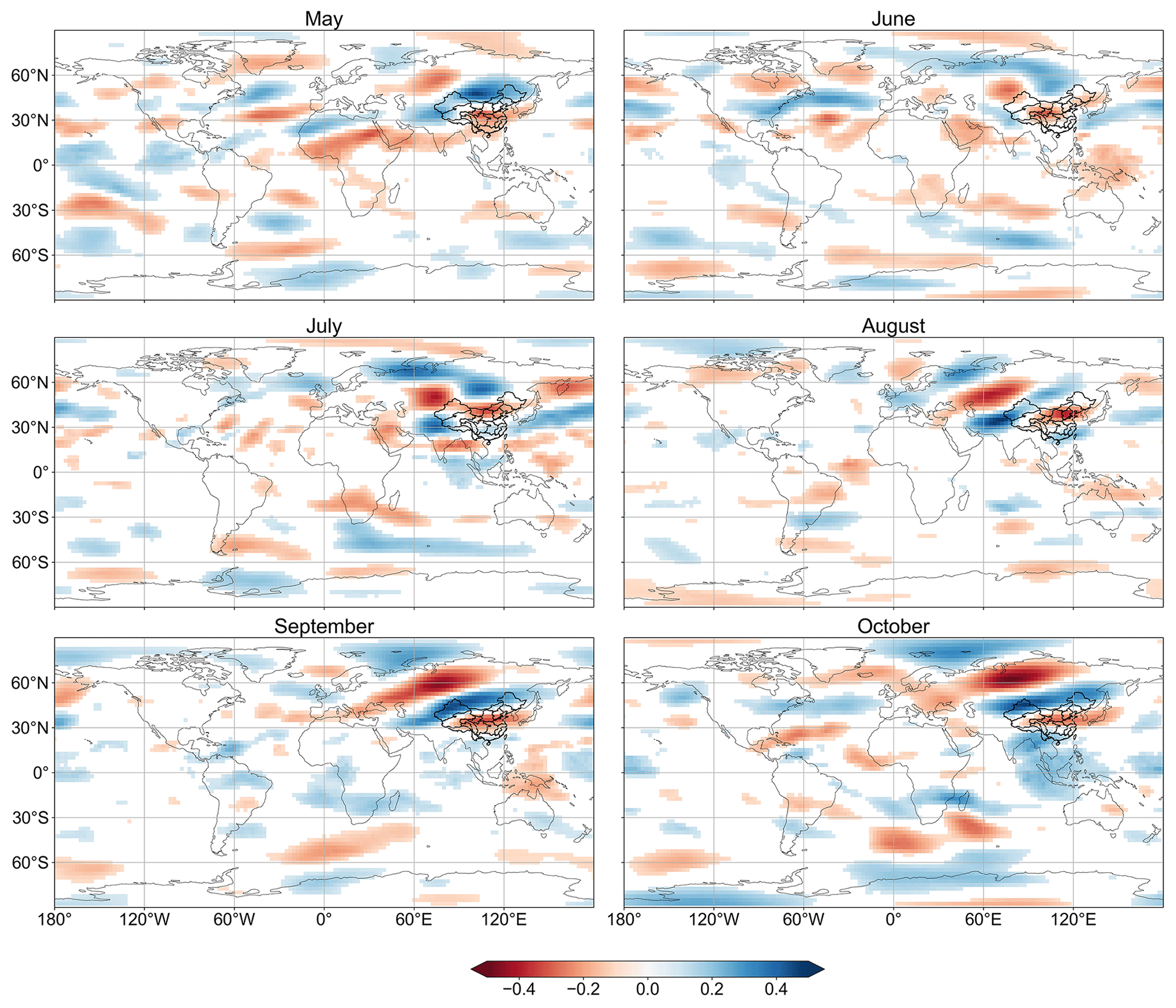
Figure 2 Correlation coefficient between pentad mean 10–60 d signals of U200 and precipitation over Region 1 (Inland rivers in Xinjiang) in different months. Correlation coefficients that are statistically significant at the 5 % level are shaded.

A CRPS skill score is then calculated by comparing the CRPS of STP-CBaM forecasts to the CRPS of reference forecasts:

$$\begin{array}{}\text{(17)}& {\mathrm{CRPS}}_{\mathrm{SS}}={\displaystyle \frac{{\mathrm{CRPS}}_{\mathrm{REF}}-\mathrm{CRPS}}{{\mathrm{CRPS}}_{\mathrm{REF}}}}\times \mathrm{100}\mathit{\%}.\end{array}$$

The reference forecasts are generated using the BJP approach to fit the observations used in the training dataset. When the CRPS skill score is 100 %, the probabilistic forecasts are the same as the observations, whereas a skill score of 0 % indicates that the probabilistic forecasts show similar accuracies compared to the cross-validated climatology. A negative skill score means that the probabilistic forecasts are inferior to the cross-validated climatology.

The forecast reliability is evaluated using the α index (Renard et al., 2010). The probability integral transform (PIT) values of probabilistic forecasts for each case i at lead time t are given as

$$\begin{array}{}\text{(18)}& {\mathit{\pi }}_{i,t}=F^{i,t}\left(o_{i,t}\right),\end{array}$$

where F^i,t( ) is the cumulative distribution function of probabilistic forecasts and o_i,t are the corresponding observations. If the ensemble forecasts are reliable, π_i,t should be uniformly distributed. The π_t values are then summarized into an α index:

$$\begin{array}{}\text{(19)}& \mathit{\alpha }=\mathrm{1.0}-{\displaystyle \frac{\mathrm{2}}{N}}\sum _{i=\mathrm{1}}^N\left|{\mathit{\pi }}_{i,t}^{*}-{\displaystyle \frac{i}{N+\mathrm{1}}}\right|,\end{array}$$

where ${\mathit{\pi }}_{i,t}^{*}$ is the sorted π_i,t in increasing order. The α index ranges from 0 to 1, and a higher α index indicates higher reliability.

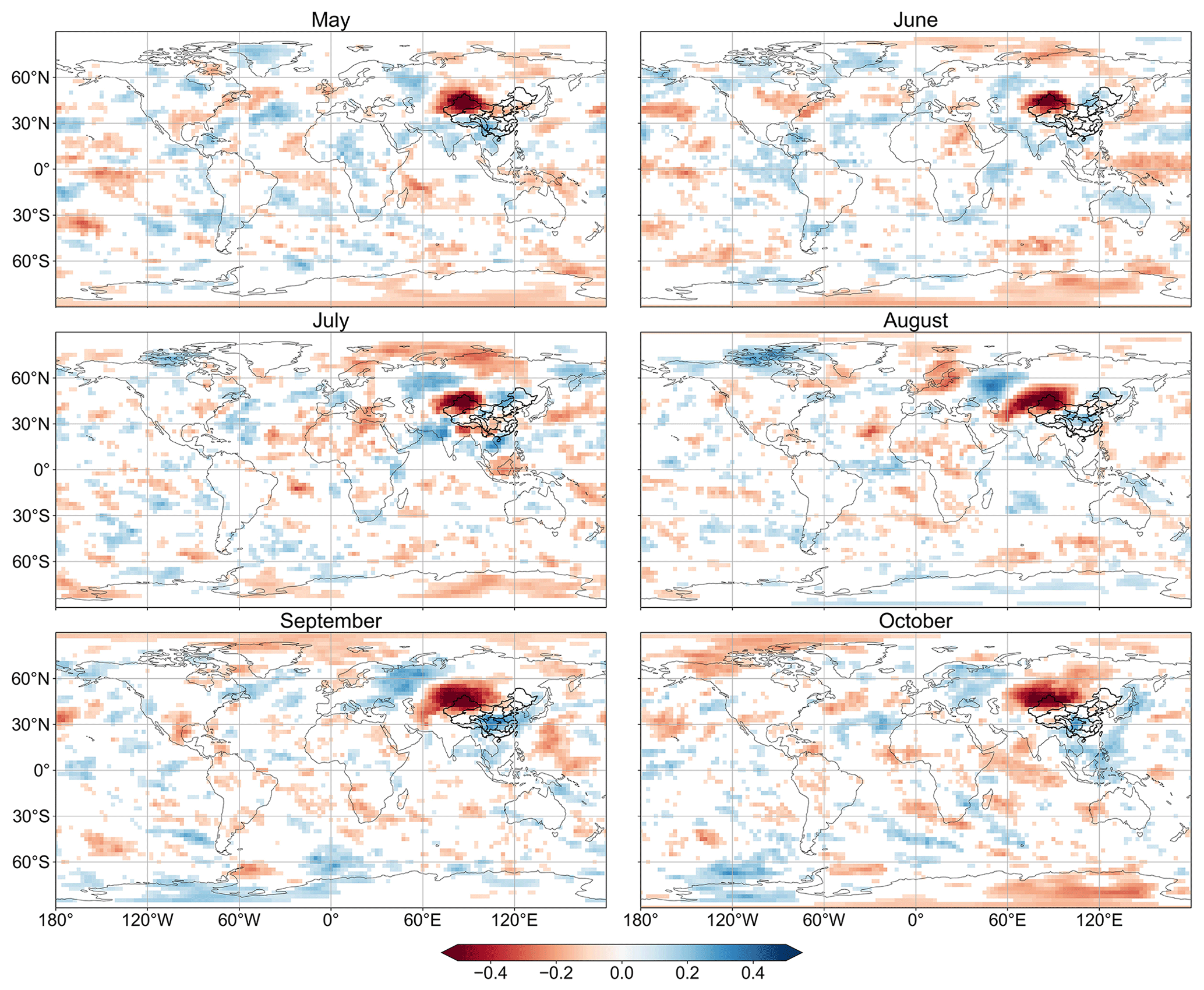
Figure 3 Same as Fig. 2 but for OLRA.

4 Results

4.1 Correlation analysis between atmospheric intraseasonal oscillation and precipitation anomalies

Figure 2 presents the correlation between pentad mean 10–60 d signals of U200 and precipitation over Region 1 (Inland rivers in Xinjiang) from May to October. The U200 signals near the Mongolian Plateau have a positive impact on precipitation anomalies over Region 1 in May, while the impact of U200 signals near the eastern Tibetan Plateau is negative. In June and July, the U200 signals in the West Siberian Plain and the Mongolian Plateau show positive correlations with precipitation anomalies. The spatial patterns of correlations between U200 signals and precipitation anomalies are similar in August, September, and October. The U200 signals near the Barents Sea and the Iranian Plateau have positive impacts on precipitation anomalies over Region 1. In comparison, U200 signals over the West Siberian Plain show strong negative correlations with precipitation anomalies in these months. The OLRA signals show similar wave patterns to other atmospheric variables (Fig. 3). The spatial patterns of correlations between U850, U200, OLRA, H200, H500, H850, and precipitation anomalies are different for each month as well (Figs. S1–S4 in the Supplement).

4.2 Skill of the ECMWF model in forecasting atmospheric intraseasonal oscillations

The forecast skill of bridging models is reliant on the forecast skill of atmospheric intraseasonal oscillations derived from dynamical models. The TCC between the ensemble mean of ECMWF-forecasted U200 intraseasonal signals and the observations in May is shown in Fig. 4. The ECMWF model shows high forecast skill in predicting U200 intraseasonal signals when the lead time is within 10 d, and the correlation coefficients are mostly over 0.7 over the globe. Although the forecast skill decreases as the lead time increases, there are still regions where the forecasted U200 signals are significantly correlated with the observations. The forecast skill of the OLRA intraseasonal oscillations is lower than that of the U200 signals (Fig. 5). High forecast skill is mostly observed near the Equator from 30 to 30^∘ E when the lead time is beyond 10 d. Similar results are also found for U850, H200, H500, and H850, where significant correlations are found mostly near the Equator at longer lead times (Figs. S5 to S8). This suggests that the forecast skill of sub-seasonal precipitation can potentially be improved by taking advantage of both skilful prediction of atmospheric intraseasonal oscillations and stable relationships between precipitation and large-scale circulations, especially for tropical regions.

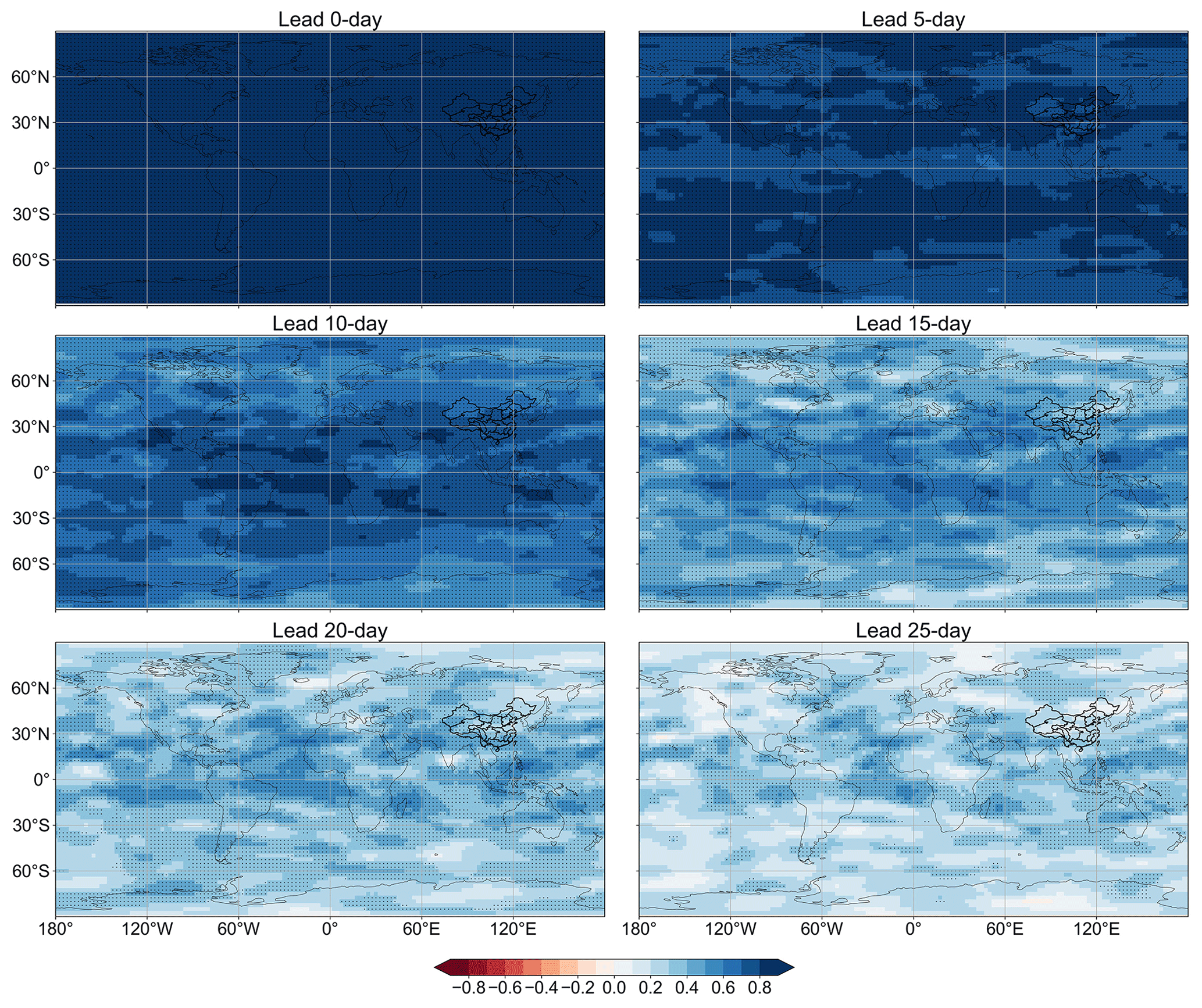
Figure 4 Temporal correlation coefficient (TCC) of the ensemble mean of U200 intraseasonal signals derived from the ECMWF model compared to the ERA5 reanalysis data in May. Correlation coefficients that are statistically significant at the 5 % level are shaded.

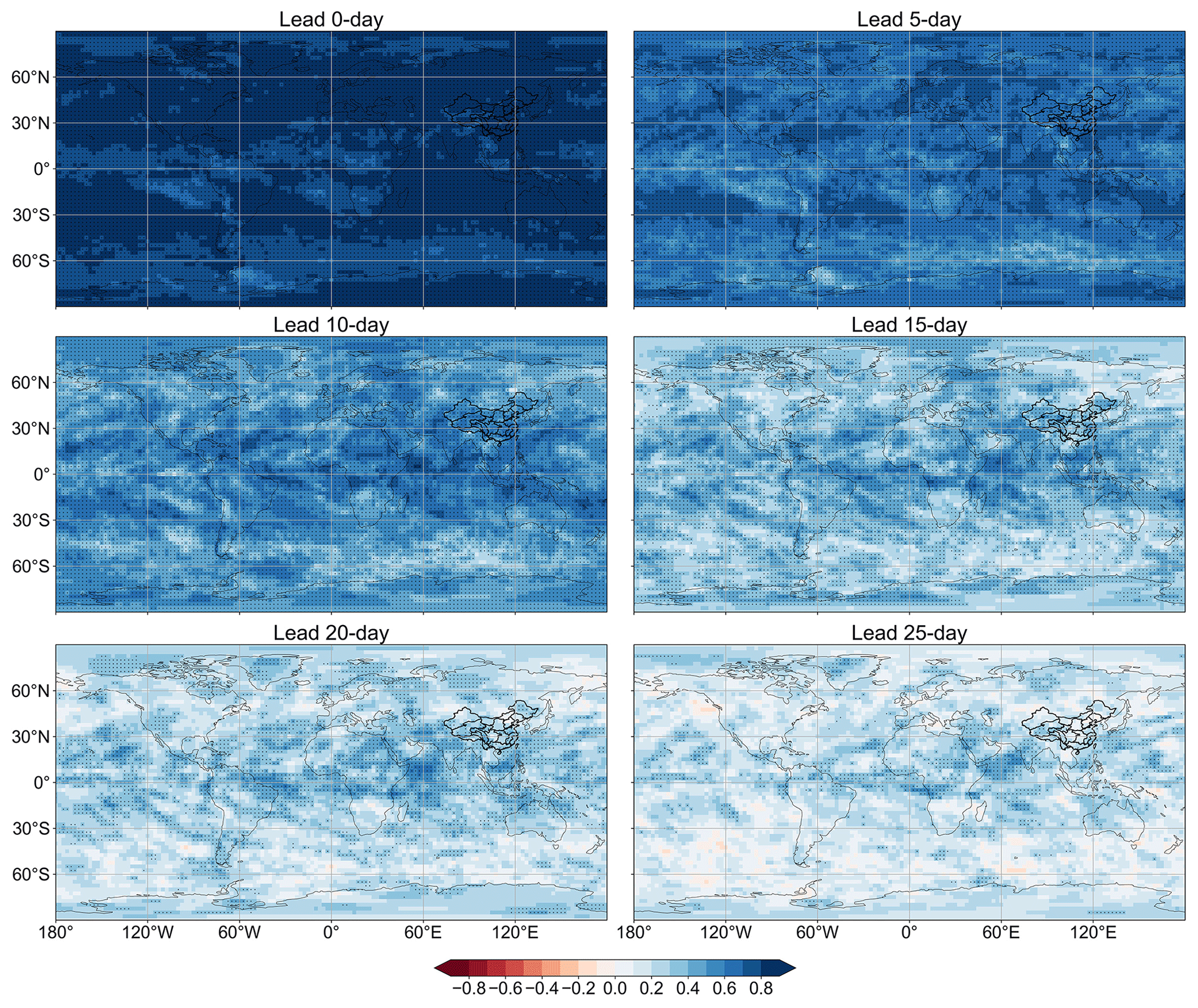
Figure 5 Same as Fig. 4 but for OLRA.

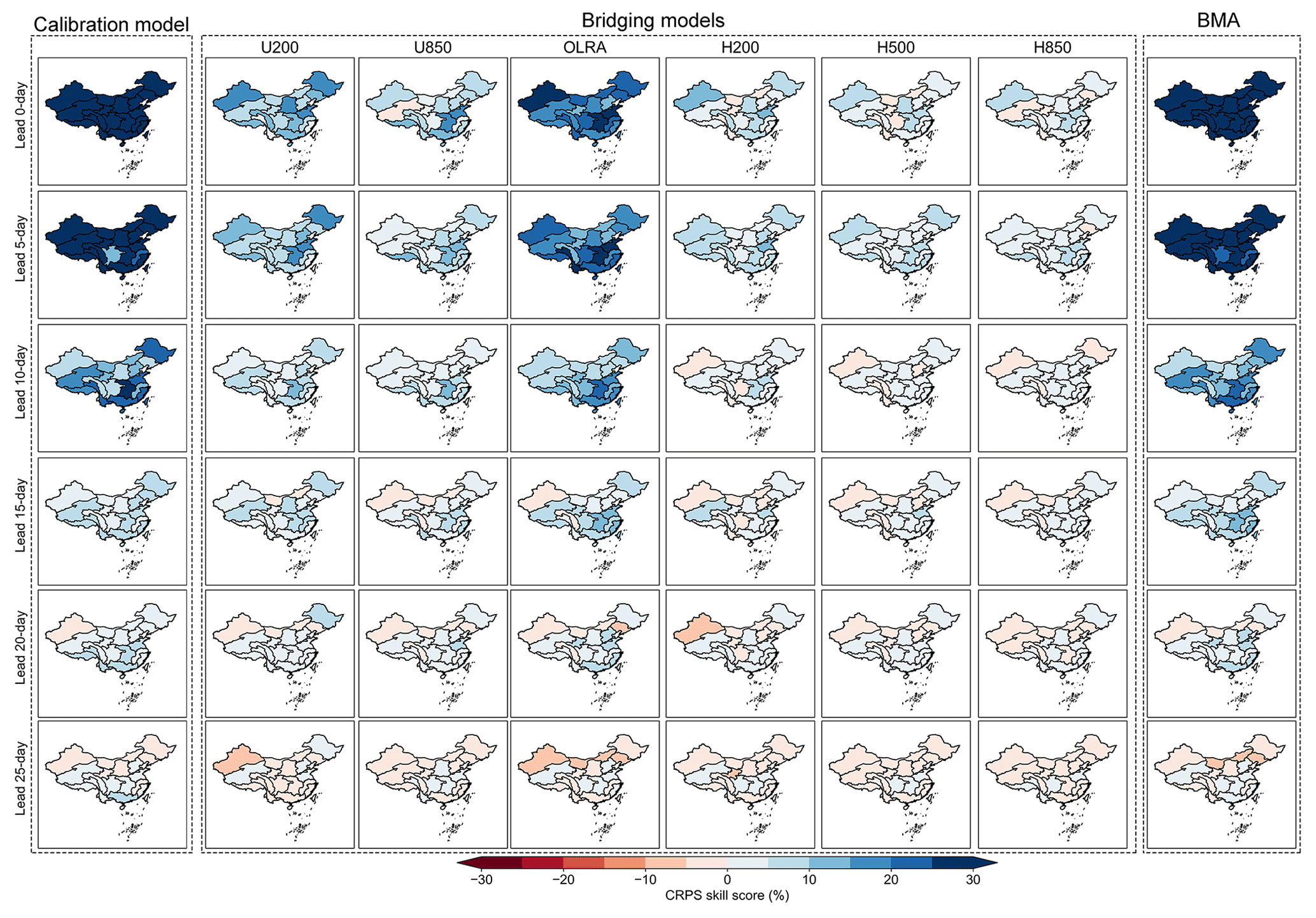
Figure 6 Spatial distribution of the CRPS skill score of the calibration model, bridging models (U200, U850, OLRA, H200, H500, H850), and merged forecasts (BMA) at different lead times in May. Publisher's remark: please note that the above figure contains disputed territories.

4.3 Skill of the calibration model, bridging models, and merged forecasts

Figure 6 presents the spatial distribution of the CRPS skill score of the calibration model, bridging models, and merged forecasts at different lead times in May. The calibration model shows the highest forecast skill compared to the bridging models at short lead times. The forecast skill of the calibrated forecasts decreases rapidly, and the CRPS skill scores are mostly below 10 % when the lead time is beyond 10 d. The forecast skill of the bridging models is higher than the calibration model in Region 10 (Huai River), Region 14 (Middle Yangtze River), and Region 17 (Southeast rivers) at a lead time of 15 d when OLRA is used as a predictor. The forecast skill of the bridging models is higher in Region 6 (Hai River) and Region 7 (Songhua River) when the OLRA and U200 signals are used separately as predictors at a lead time of 20 d. The merged forecasts take advantage of both the calibration model and the bridging models. Figure 7 shows the boxplots of the CRPS skill scores of the calibration model, bridging models (U200, U850, OLRA, H200, H500, H850), and merged forecasts (BMA) at different lead times in May. The distribution of the CRPS skill score of the merged forecasts is similar to the calibration model at a lead time of 0 d. The minimum CRPS skill score of the merged forecasts is over 20 % in Region 13 (Yangtze River) at a lead time of 5 d, higher than both the calibration model and the bridging models. The bridging models, which use the U200 and OLRA as predictors, show a higher minimum CRPS skill score compared to the calibration model and other bridging models at a lead time of 10–15 d. The distributions of the CRPS skill score of the calibration model, bridging models, and BMA-merged forecasts are similar at longer lead times.

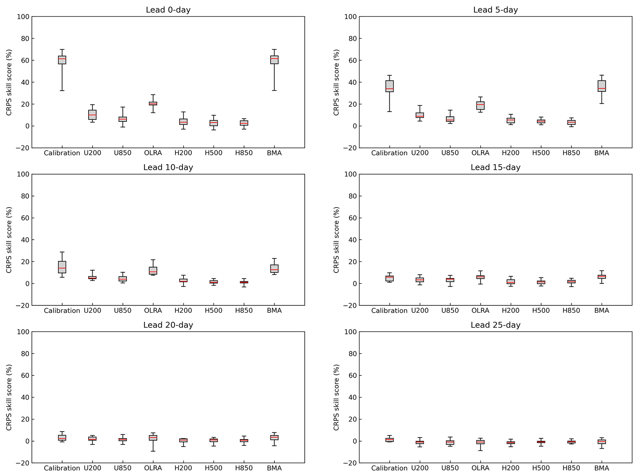
Figure 7 Boxplots of the CRPS skill score of the calibration model, bridging models (U200, U850, OLRA, H200, H500, H850), and merged forecasts (BMA) at different lead times in May. The red lines are the 50th percentiles, the top and bottom of each box are the 75th and 25th percentiles, and the whiskers are the maximum and minimum skill scores.

Figure 8 shows the distribution of model weights at different lead times for Region 1 (Inland rivers in Xinjiang) in May. The weights are rather stable at short lead times, when more than 90 % of the total weights are assigned to the calibration model. Similar results are also found in other regions and months (not shown). The weights of the calibration model decrease rapidly when the lead time is beyond 10 d. More weights are assigned to U200 and OLRA at longer lead times. This is mostly consistent with the distribution of CRPS skill scores shown in Fig. 7. The CRPS skill scores of the U200- and OLRA-based bridging models are higher than the calibration model and other bridging models, especially when the lead time is between 10 and 20 d. This indicates that the U200 and OLRA signals are more useful in predicting sub-seasonal precipitation anomalies compared to other large-scale atmospheric circulation variables.

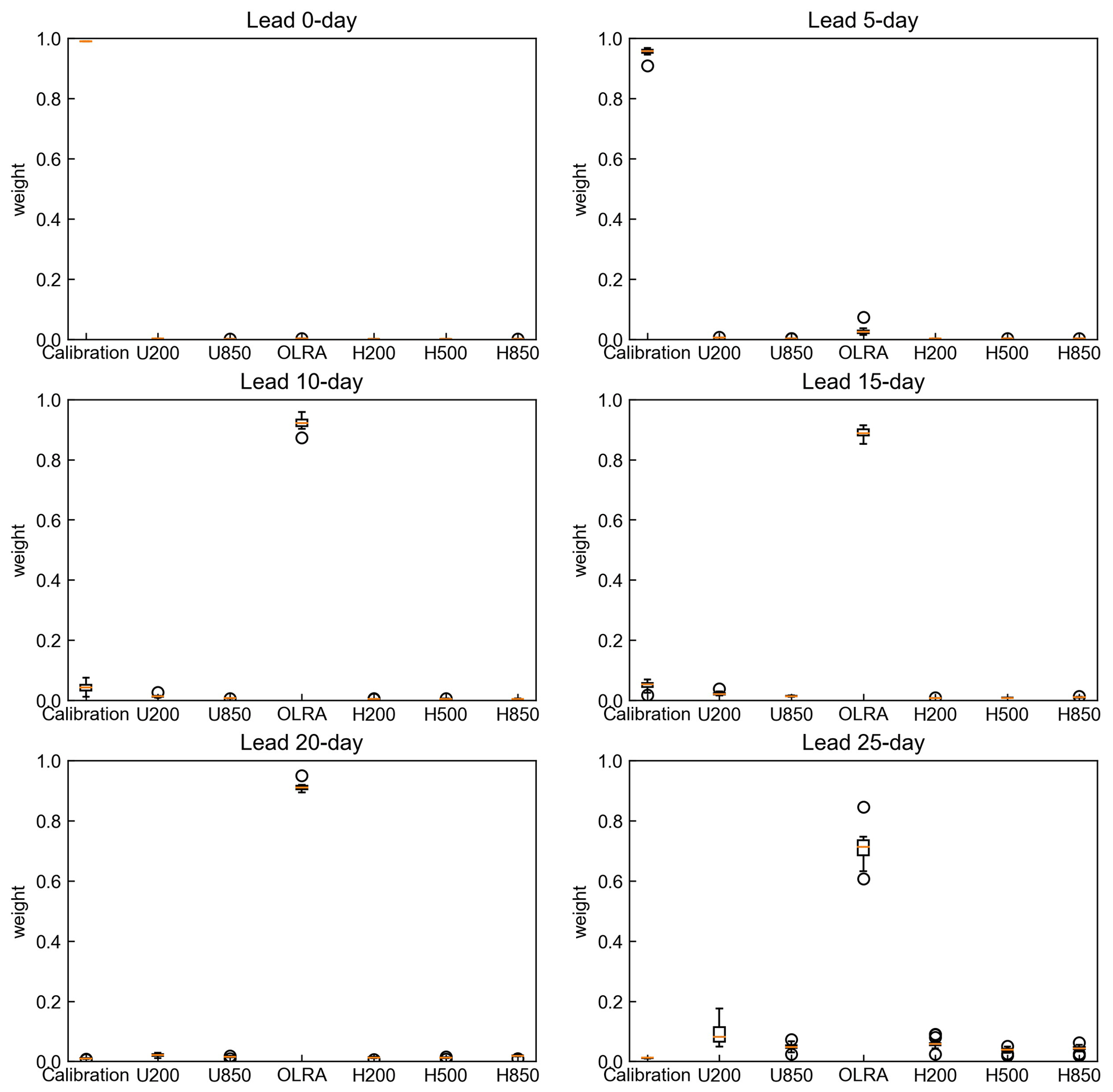
Figure 8 Boxplots showing the distribution of model weights at different lead times in cross-validation for Region 1 (Inland rivers in Xinjiang) in May.

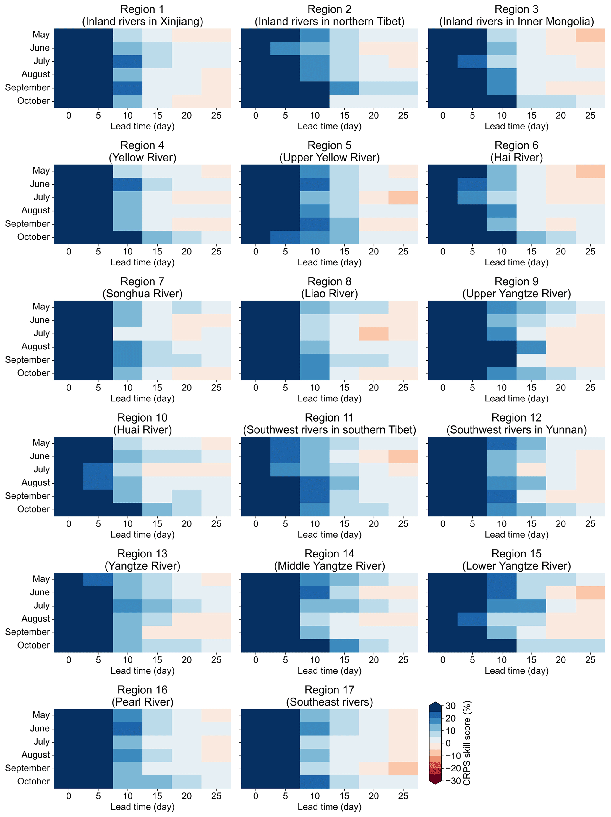
Figure 9 presents the CRPS skill score of merged forecasts at different lead times from May to October. In general, the forecast skill shows regional, monthly, and lead-time-dependent patterns. The merged forecasts show higher skill in predicting sub-seasonal precipitation anomalies over Region 16 (Pearl River) than other regions. The CRPS skill scores are positive for all months at lead times of 0–20 d. This is mainly due to the higher prediction skill of OLRA in these regions, as shown in Fig. 5. In addition, the merged forecasts show the highest skill in October, when positive skill scores are found over 14 hydroclimatic regions for all lead times except in Region 1 (Inland rivers in Xinjiang), Region 7 (Songhua River), and Region 8 (Liao River). In comparison, positive skill scores are found only over three hydroclimatic regions for all lead times (Region 1, Inland rivers in Xinjiang, Region 13, Yangtze River, and Region 14, Middle Yangtze River) in July.

Figure 9 CRPS skill score of merged forecasts at different lead times from May to October.

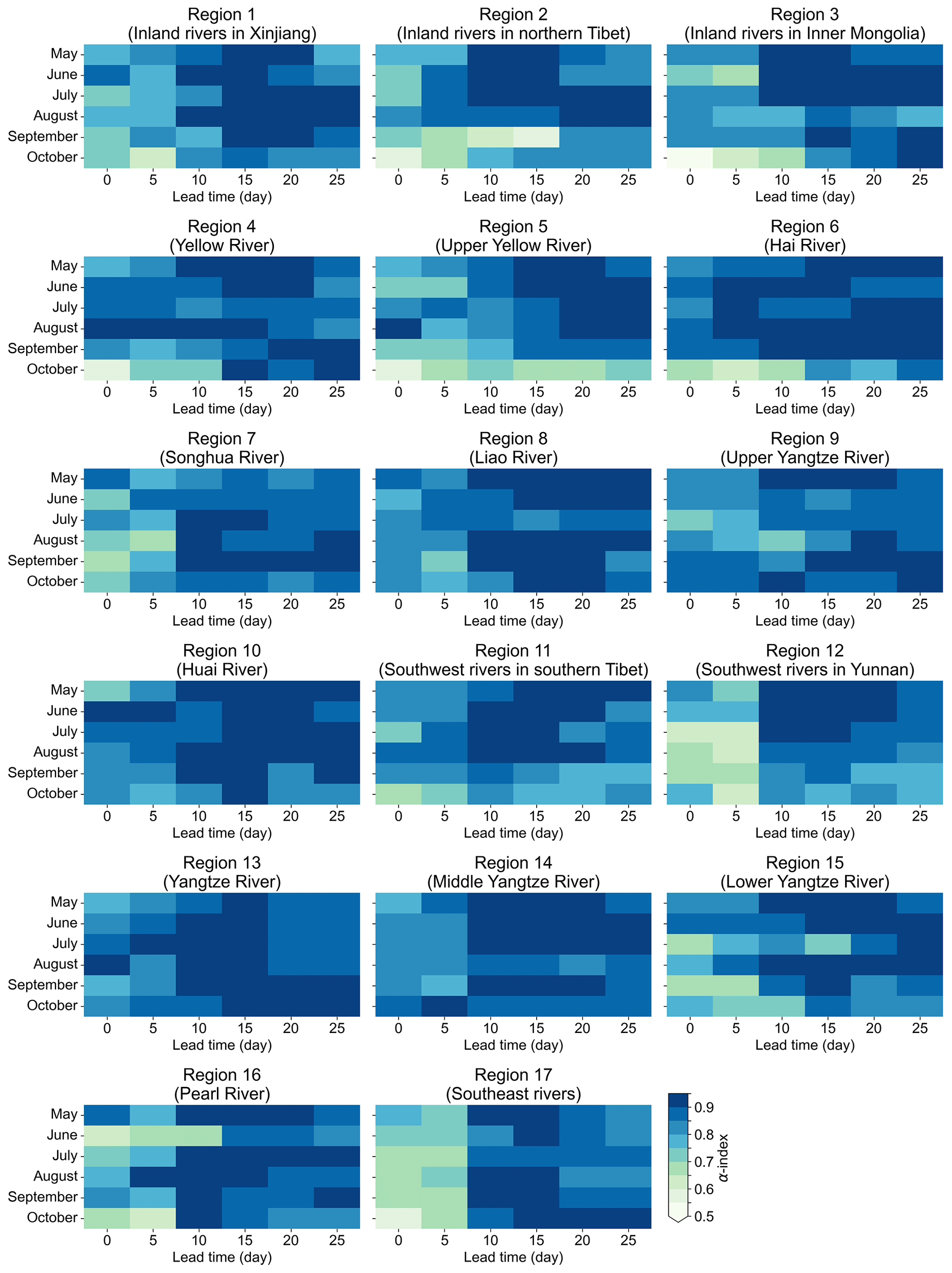
The α indices of merged forecasts at different lead times are shown in Fig. 10. The α index is around 0.7 at short lead times, suggesting that the forecasts have a relatively low reliability. The α index is over 0.85 when the lead time is beyond 10 d for all hydroclimatic regions and lead times. This indicates that the merged forecasts have a higher reliability at longer lead times. To figure out the relatively low reliability at short lead times, we analyse the merged forecasts over Region 3 (Inland rivers in Inner Mongolia) in May at a lead time of 0 d. The α index of the merged forecasts is around 0.6, suggesting that the merged forecasts have a low reliability. We also investigate the model weights of calibrated forecasts and bridging forecasts. The results suggest that the calibrated forecasts are more important than the bridging forecasts, while the cross-validated model weights are over 0.95. This suggests that the low reliability of merged forecasts is mostly caused by the low reliability of calibrated forecasts. Figure S9 presents the quantile ranges of calibrated forecasts and merged forecasts against time. The quantile ranges of both the calibrated forecasts and merged forecasts are small, suggesting that the forecasts are too narrow (too confident).

Figure 10 Same as Fig. 9 but for the α index.

5 Discussion

5.1 Discussion of forecast skill

Though the STP-CBaM model displays a good ability to generate skilful and reliable sub-seasonal precipitation forecasts over China, the forecast skill shows great diversity in different regions, months, and lead times. The calibration model shows the highest forecast skill compared to the bridging models for all regions and all months when the lead time is within 5 d (Figs. S10–S14). The U200- and OLRA-based bridging models outperform the calibration model and the other bridging models when the lead time is beyond 10 d in certain months and in certain regions. This may be explained by the strong relationship between U200, OLRA, and precipitation anomalies and the forecast skill of U200 and OLRA in the ECMWF model in these regions (Figs. S5–S8).

However, we also note that there are several regions where the forecast skill of the calibration model is higher than the bridging models at longer lead times. This may be caused by the auto-correlations of the sub-seasonal precipitation anomalies defined in this study. In our data processing section, the observed anomalies before the forecast initial date are used to make enough data for the running mean. Thus, the predictand is not purely based on the ECMWF raw forecasts. The observational data are also introduced. The preceding observed precipitation anomalies may provide useful forecast information when the auto-correlations are high.

In addition, the limited forecast skill of large-scale circulations at mid to high latitudes in dynamical models may contribute to the limited forecast skill of bridging models as well. To figure out the potential skill of the STP-CBaM method in predicting sub-seasonal precipitation anomalies, we use the pth 10–60 d signal of the atmospheric field derived from the ERA5 reanalysis dataset as a predictor for the bridging model instead of the atmospheric field derived from the ECMWF model. Thus, the potential forecast skill is based on ERA5 reanalysis data, while the practical forecast skill is based on the ECMWF model. Figure 11 compares the potential CRPS skill score (based on the ERA5 reanalysis) and the practical CRPS skill score (based on the ECMWF model) of merged forecasts over China. The potential CRPS skill scores are similar to the practical CRPS skill scores as the precipitation forecasts derived from the ECMWF model have a high accuracy at short lead times. The potential CRPS skill scores are much higher than the practical CRPS skill scores at longer lead times. This indicates that the forecast skill will be greatly improved when the atmospheric field is well predicted in the GCMs.

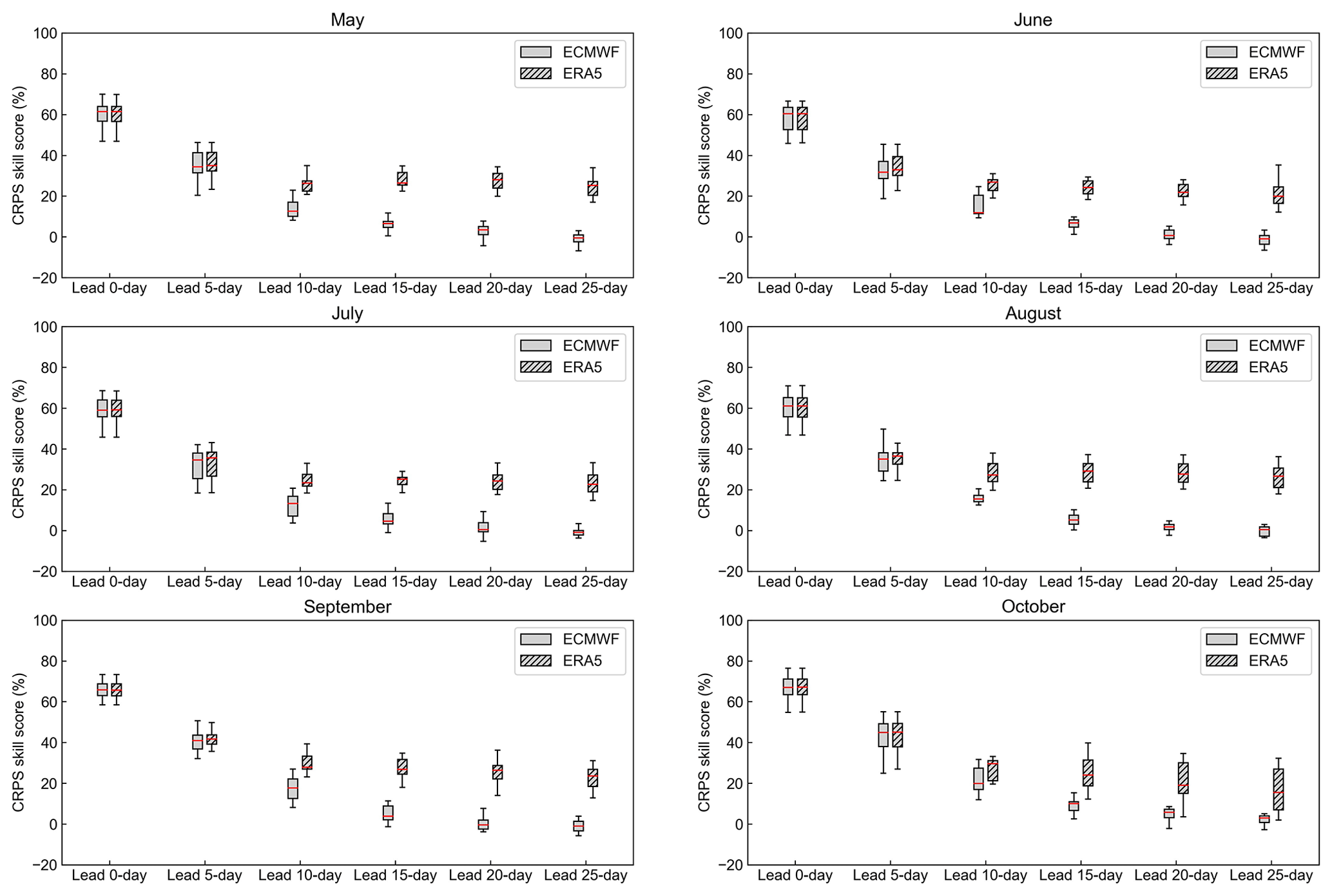
Figure 11 Practical CRPS skill score of merged forecasts based on the ECMWF model (solid) and potential CRPS skill score based on ERA5 reanalysis (hatched). The red lines are the 50th percentiles, the top and bottom of each box are the 75th and 25th percentiles, and the whiskers are the maximum and minimum skill scores.

We also note that the weights do not always match the skill patterns. In this study, the posterior distributions of model weights are assigned by a model's predictive ability rather than fitting ability. Indeed, there is much literature in support of using predictive performance measures for model choice and combination based on the idea that a model is only as good as its predictions (Stock and Watson, 2006; Eklund and Karlsson, 2007). Thus, the CRPS skill score is not used when inferring model weights. This may lead to the discrepancy between the model weights and the forecast skill score, especially when none of the models shows high predictive skill.

5.2 Limitations and future work

In this study, we aim at investigating the capability of dynamical models to improve the forecast skill of sub-seasonal precipitation anomalies using large-scale circulations as predictors. The bridging models are built based on the concurrent relationships between atmospheric intraseasonal oscillations and precipitation anomalies. Thus, the forecast skill of bridging models is highly reliant on the forecast skill of atmospheric intraseasonal oscillations derived from dynamical models. In the future, the lagged relationships between atmospheric intraseasonal oscillations and precipitation anomalies will be considered to further improve sub-seasonal precipitation forecast skill. Although the forecast skill of the calibration model is high at short lead times, the results also suggest that the calibrated forecasts are too narrow (too confident). We would like to focus on improving the forecast reliability, especially at short lead times, in the future.

Meanwhile, we define the predictors using the STPM for each month and each hydroclimatic region. Intraseasonal climate indices, such as the MJO index and the BSISO index, have not been considered yet. Recently, Zhu et al. (2023) proposed two sets of novel indices based on the compound zonal displacements of the South Asia high (SAH) and the western Pacific sub-tropical high (WPH) to monitor and predict the intraseasonal variation of Meiyu. These climate indices will be introduced in the bridging models to investigate the potential improvement of the forecast skill.

In addition, we mainly focus on the prediction of intraseasonal (10–60 d) precipitation anomalies in this study. However, previous studies suggested that the intraseasonal component may only account for 7 % of the total variability in north-eastern China, while the seasonal component accounted for nearly 70 %. Thus, the relationships between seasonal precipitation anomalies and large-scale circulation patterns should also be investigated in these regions in the future.

6 Conclusions

In this study, we develop a STP-CBaM method to improve probabilistic sub-seasonal precipitation forecast skill over 17 hydroclimatic regions in China. The STP-CBaM method takes advantage of both dynamical models and statistical models. The calibration model is built by calibrating pentad mean precipitation anomalies derived from the ECMWF model. Bridging models are built by defining potential predictors using the spatial–temporal projection method (STPM). The calibration model and bridging models are merged through the Bayesian modelling averaging (BMA) method. Our results suggest that the forecast skill of the calibration model is higher compared to the bridging models when the lead time is within 5–10 d. The U200- and OLRA-based bridging models outperform the calibration model when the lead time is beyond 10 d in certain months and certain regions. The BMA-merged forecasts take advantage of both the calibration model and the bridging models. The BMA weights are rather stable at short lead times, where over 90 % of the total weights are assigned to the calibration model. More weights are assigned to the U200- and OLRA-based bridging models when the lead time is beyond 10 d. The results of the α index suggest that BMA-merged forecasts are reliable at longer lead times. Some improvements to reliability are still needed at shorter lead times.