Bias-blind and bias-aware assimilation of leaf area index into the Noah-MP land surface model over Europe

Data assimilation (DA) of remotely sensed leaf area index (LAI) can help to improve land surface model estimates of energy, water, and carbon variables. So far, most studies have used bias-blind LAI DA approaches, i.e. without correcting for biases between model forecasts and observations. This might hamper the performance of the DA algorithms in the case of large biases in observations or simulations or both. We perform bias-blind and bias-aware DA of Copernicus Global Land Service LAI into the Noah-MP land surface model forced by the ERA5 reanalysis over Europe in the 2002–2019 period, and we evaluate how the choice of bias correction affects estimates of gross primary productivity (GPP), evapotranspiration (ET), runoff, and soil moisture.

In areas with a large LAI bias, the bias-blind LAI DA leads to a reduced bias between observed and modelled LAI, an improved agreement of GPP, ET, and runoff estimates with independent products, but a worse agreement of soil moisture estimates with the European Space Agency Climate Change Initiative (ESA CCI) soil moisture product. While comparisons to in situ soil moisture in areas with weak bias indicate an improvement of the representation of soil moisture climatology, bias-blind LAI DA can lead to unrealistic shifts in soil moisture climatology in areas with strong bias. For example, when the assimilated LAI data in irrigated areas are much higher than those simulated without any irrigation activated, LAI will be increased and soil moisture will be depleted. Furthermore, the bias-blind LAI DA produces a pronounced sawtooth pattern due to model drift between DA updates, because each update pushes the Noah-MP leaf model to an unstable state. This model drift also propagates to short-term estimates of GPP and ET and to internal DA diagnostics that indicate a suboptimal DA system performance.

The bias-aware approaches based on a priori rescaling of LAI observations to the model climatology avoid the negative effects of the bias-blind assimilation. They retain the improvements in GPP anomalies from the bias-blind DA but forego improvements in the root mean square deviations (RMSDs) of GPP, ET, and runoff. As an alternative to rescaling, we discuss the implications of our results for model calibration or joint parameter and state update DA, which has the potential to combine bias reduction with optimal DA system performance.

1 Introduction

Vegetation plays a major role in climatic interactions between the land surface and the atmosphere. Via transpiration and photosynthesis, it contributes to the exchange of energy, water, and carbon at the surface, and it links the moisture in the deeper soil layers to the atmosphere (Bonan, 2019). On short timescales, these exchanges can impact precipitation and atmospheric circulation (Betts et al., 1996; Miralles et al., 2016). On longer timescales, the net uptake of CO₂ by vegetation (Friedlingstein et al., 2022) might be decreased due to climate change, contributing to rising CO₂ levels (Green et al., 2019; Walker et al., 2021). Land surface models (LSMs) are often used to estimate these exchange fluxes as part of earth system models or as the land component in numerical weather prediction (NWP) systems (e.g. Balsamo et al., 2009; Lawrence et al., 2019; Skamarock et al., 2021). An accurate description of vegetation in LSMs can therefore improve estimates of evapotranspiration (ET) in NWP (Boussetta et al., 2013), or it can be used to estimate how vegetation will develop under a changed climate (Laanaia et al., 2016) and how this affects the land carbon sink (Tharammal et al., 2019a, b; Green et al., 2019).

However, the dynamic simulation of vegetation in global LSMs is still in its infancy and has large uncertainties, especially in dry climates (Fox et al., 2018; Mahmud et al., 2021). Satellite-based vegetation data assimilation (DA) can be used to reduce the uncertainties of the vegetation-related LSM estimates. Satellite-derived leaf area index (LAI) is commonly used for DA, because it can be derived from optical sensors fairly accurately (Fang et al., 2019) and is also available as a model state variable in several land surface models with a dynamic vegetation component. Satellite LAI has, for example, been assimilated into the Interactions between Soil Biosphere Atmosphere (ISBA) LSM (Sabater et al., 2008; Barbu et al., 2014; Fairbairn et al., 2017; Albergel et al., 2017; Mucia et al., 2020), the Noah LSM with multiparameterisation options (Noah-MP; e.g. Kumar et al., 2019b, 2021; Rahman et al., 2022b; Nie et al., 2022), the Community Land Model (CLM; e.g. Fox et al., 2018; Ling et al., 2019), and the Carbon-Tiled ECMWF Scheme for Surface Exchange over Land (CTESSEL; e.g. Jarlan et al., 2008). Alternatives are, for example, to use microwave brightness temperatures to simultaneously update the soil moisture and LAI (Sawada and Koike, 2014; Sawada et al., 2015) or to use microwave vegetation optical depth (VOD) retrievals to update LAI (Kumar et al., 2020, 2021).

The most commonly used methods for assimilating LAI into LSMs are based on the Kalman filter. A fundamental assumption of these methods is that modelled and observed LAI are unbiased. Yet, in reality, biases nearly always exist. This includes biases of both model estimates and observations with respect to the unknown true value and the bias between the model estimates and observations themselves. If the observations are closer to the true value than the model estimates, a “bias-blind” DA (Dee, 2005) is able to correct the model bias to some extent, because it pulls the model closer towards the observations and hence the true values. This comes at the risk of introducing unintended negative side effects. For example, it is possible that other processes (e.g. transpiration) are only represented well for a biased model climatology. Large updates in a subset of the model state might therefore propagate to other model components, which can negatively affect estimates of state variables and fluxes of these processes (De Lannoy et al., 2007b; Crow et al., 2020). Furthermore, if the model equilibrium state is far away from the observations, the updates towards the observations might not persist for long. Instead, the model drifts back towards its original state, leading to a sawtooth-like pattern in the resulting time series and potentially also to unrealistic water, carbon, and energy flux estimates (Dee, 2005; De Lannoy et al., 2007b). Changes in observation frequency or periodically missing data may then also introduce spurious trends into the analysis (Dee, 2005).

Most LAI assimilation studies so far have used bias-blind approaches, i.e. they did not apply any bias correction methods to account for existing biases between modelled LAI and observed LAI. This is often justified by the argument that the bias is caused by model deficiencies (e.g. Fairbairn et al., 2017; Fox et al., 2018; Albergel et al., 2020). Nonetheless, there are indications that the presence of bias affects the performance of LAI assimilation. Albergel et al. (2017, 2020) noticed systematic drifts towards the previous model estimate on days without observations. Kumar et al. (2019b) and Mocko et al. (2021) also found model drifts leading to sawtooth patterns in analysed LAI when using the Noah-MP LSM with dynamic vegetation.

Various techniques have been used to limit the negative effects listed above. Albergel et al. (2017, 2020) and Mucia et al. (2021) additionally assimilated surface soil moisture retrievals. This additional constraint can help to prevent negative side effects of the LAI DA on the model hydrology, but only in regions and periods where sufficient soil moisture observations are available. Kumar et al. (2019b), Mocko et al. (2021) and Rahman et al. (2022b) interpolated their assimilated LAI product to daily values to prevent issues due to different observation frequencies and to limit the drift towards the original equilibrium state. Fox et al. (2018) adaptively inflated the model error in the case of large bias between modelled LAI and the observations. The latter two techniques force the analysis to stay close to the observations, which begs the question of whether it might be more suitable to use a direct insertion approach or to prescribe the observed LAI instead of modelling it dynamically, as for example done by Maertens et al. (2021) and Huang et al. (2022).

Bias-aware data assimilation is another possible avenue to handle bias between models and observations. This includes a priori rescaling approaches, which map the observations into the model space based on a priori estimates of model and observation statistics (e.g. Reichle and Koster, 2004; Jarlan et al., 2008; Khaki et al., 2020), or online approaches which adaptively estimate dynamic bias corrections (e.g. Derber and Wu, 1998; Dee, 2005; De Lannoy et al., 2007a). Only a few studies have considered bias-aware approaches based on rescaling for LAI DA (Jarlan et al., 2008; Khaki et al., 2020). However, so far, no study has directly compared bias-blind and bias-aware LAI DA.

In this article, we compare bias-blind LAI DA with bias-aware LAI DA using two a priori rescaling techniques commonly used for satellite DA. More specifically, we assimilate Copernicus Global Land Service (CGLS) LAI (Smets et al., 2019) into the Noah-MP model (Niu et al., 2011) forced with the fifth-generation European Center for Medium-Range Weather Forecasts (ECMWF) Reanalysis (ERA5; Hersbach et al., 2020) reanalysis over Europe, and we quantify the effects of bias-blind and bias-aware DA on vegetation and surface water flux and state estimates.

A detailed description of the model, data, and rescaling approaches used can be found in Sect. 2. Section 3 shows the impacts of the bias-blind DA on the vegetation and hydrology model estimates, evaluates the results using independent reference datasets, and compares the model simulations to in situ data from Majadas, Spain. Additionally, we provide an analysis of the sawtooth pattern in the bias-blind DA and of internal DA diagnostics. We discuss the implications of our results for LAI DA design and model calibration in Sect. 4. A summary of our main conclusions is given in Sect. 5.

2 Data and methods

2.1 Land surface model

We used version 4.0.1 of the Noah-MP LSM (Niu et al., 2011; Yang et al., 2011) with dynamic vegetation as implemented in the NASA Land Information System (LIS; Kumar et al., 2006; Peters-Lidard et al., 2007)). The Noah-MP LSM is based on the Noah LSM, which is widely used for land surface modelling and DA on a regional to global scale (e.g. Rodell et al., 2004; Kumar et al., 2014, 2019a; Maertens et al., 2021). Noah-MP includes a multitude of optional improvements for snow, water, and vegetation modelling. It has already been used to update LAI using optical satellite imagery (Kumar et al., 2019b; Erlingis et al., 2021; Rahman et al., 2022b) and microwave vegetation optical depth (Kumar et al., 2020, 2021).

The dynamic vegetation model of Noah-MP is based on the vegetation model in the Biosphere–Atmosphere Transfer Scheme (BATS) model (Dickinson et al., 1998). In this model, gross primary productivity (GPP) is allocated to the four vegetation carbon pools (leaves, non-woody stems, wood, and fine roots) in each simulation step. LAI is calculated from leaf carbon mass by multiplying with a vegetation-type-dependent specific leaf area. It can feed back to other model state variables and fluxes via its effect on photosynthesis, evapotranspiration (ET), precipitation interception, and runoff. Changes in LAI can therefore also induce changes in the model hydrology. A more detailed overview of the dynamic leaf model in Noah-MP is given in Appendix A.

Maps of soil texture and land cover, and multiple parameters based on these, are required as input to the model and were taken from the NCCS Dataportal (https://portal.nccs.nasa.gov/lisdata_pub/data/PARAMETERS/, last access: 3 November 2023; Tian et al., 2008). We used the STATSGO-FAO (State Soil Geography – Food Agricultural Organisation) soil texture map produced by the National Center for Atmospheric Research (NCAR). For vegetation, we used the IGBP-NCEP (International Geosphere-Biosphere Programme – National Centers for Environmental Prediction) land cover map based on Friedl et al. (2002). This map classifies some pixels in France, Spain, Ireland and Germany as evergreen broadleaf forests, which the model interprets as tropical rainforests. We therefore replaced these pixels with the land cover class from the University of Maryland (UMD) land cover map (Hansen et al., 2000). The soil texture and land cover maps are available on a 0.01^∘ regular grid and were upscaled to a 0.25^∘ grid using the largest fraction within a model grid cell.

As forcing, Noah-MP requires the lowest-level atmospheric model (about 10 m a.g.l. – above ground level) air temperature, wind speed, specific humidity and pressure, the downwelling fluxes of short-wave and long-wave radiations, as well as precipitation (partitioned into solid and liquid phases). We used data from ERA5, the latest ECMWF reanalysis, for this purpose. The ERA5 forcings have an original resolution of 31 km and were mapped to a 0.25^∘ regular grid. The initial model state was obtained from a 30-year deterministic spin-up run, cycling three times with the forcing data from 2000 to 2010, followed by 2 years of ensemble spin-up from 2000 to 2002.

The model domain in this study covers Europe as well as parts of northern Africa and the Middle East on a regular grid with 0.25^∘ resolution (ranging from 29.875^∘N, −11.375^∘E to 71.625^∘N, 40.125^∘E). It includes a wide range of climates and vegetation types, from tundra and boreal forests in Scandinavia to the Sahara Desert. We performed the model simulations from 2002 through 2019, using a 15 min simulation time step and outputting daily averages centred at 00:00 UTC.

2.2 LAI observations

We assimilated the Copernicus Global Land Service (CGLS) satellite LAI product version 2 derived from the Project for On-Board Autonomy – Vegetation (PROBA-V) and the Satellite Pour l’Observation de la Terre – Vegetation (SPOT-VGT) (Verger et al., 2014). This product has been used for LAI DA before, e.g. by Barbu et al. (2014), Albergel et al. (2017), and Mucia et al. (2020). The 1 km resolution CGLS LAI product is provided as one image every 10 d composed from an adaptive window of 15 to 60 d, depending on the availability of valid measurements (Smets et al., 2019). We masked out gap-filled values and upscaled the data to 0.25^∘ resolution by averaging over all observations within one model grid cell. In contrast to Kumar et al. (2019b), we did not interpolate LAI to daily values. In this way, we (i) did not introduce observation error autocorrelations, (ii) allowed our results to be generalizable to LAI datasets (or proxy datasets as used in Kumar et al., 2020; Mucia et al., 2021) with less frequent observations or changes in observation frequency, and (iii) could investigate whether the filter efficiently interpolates and operates as intended (or assumed). We assimilated the aggregated data every 10 d at 00:00 UTC where and when they were available.

2.3 Data assimilation

We used a one-dimensional ensemble Kalman filter (EnKF; Evensen, 2003) for assimilating the CGLS LAI observations into the Noah-MP LSM. The EnKF is a two-step procedure. First, the model simulates the land surface state x^f(t) at the next assimilation time step t (forecast). Then, the model state is updated to agree better with the observations y(t), resulting in the analysis x^a(t). The magnitude of the update (increment) depends on the innovations (observation minus forecast) and the relative sizes of the forecast and observation error variances. In a properly configured DA system, the normalised innovations (innovations divided by the total error standard deviation) should be temporally uncorrelated and follow a standard normal distribution, i.e. the innovation sequence should be a white noise sequence with zero mean and unit standard deviation (Desroziers et al., 2005). Following prior work on LAI DA with Noah-MP (Kumar et al., 2019b; Mocko et al., 2021; Rahman et al., 2022b, a), we used the EnKF to update the model LAI, i.e. the state vector consisted only of LAI. For the reasons discussed in Sect. 4.4, we chose not to add soil moisture to the updated state vector.

In the EnKF, the forecast error is estimated based on an ensemble of model simulations. We used 24 ensemble members, one of which was driven by the original forcing data, while the others were driven by perturbed radiation and precipitation forcing data. Additionally, we applied normally distributed perturbations to the model LAI state variable with a mean of zero and a standard deviation of 0.01 m² m⁻² every 3 h for the 23 perturbed ensemble members. The unperturbed ensemble member was used to correct for perturbation biases due to nonlinear processes using the method described by Ryu et al. (2009). All of the perturbation specifications and the observation error standard deviation of 0.05 m² m⁻² were set following Kumar et al. (2019b).

To remove systematic differences between the modelled and observed LAI, we implemented either of two a priori rescaling methods: climatological cumulative distribution function (CDF) matching and a seasonal rescaling of the first and second moments. CDF matching is commonly used for soil moisture DA when the various seasons are not distinguished (e.g. Reichle and Koster, 2004; Drusch et al., 2005; Draper et al., 2012; Parrens et al., 2014; Barbu et al., 2014). It attempts to correct the biases in all statistical moments by nonlinearly transforming the observation data such that the empirical CDF of the rescaled LAI data matches the empirical CDF of the modelled data. To estimate the empirical CDFs for each grid cell individually in a robust way, we opted to bin the data between the 2nd and 98th percentiles. We then estimated the CDF by linearly interpolating the percentile values between the bin edges. For values outside the interval [2, 98], the lines for the first and last bin were extrapolated to 0 and 100, respectively. The resulting curve was discretised into 100 equally spaced bins over the full data range for use in the numerical rescaling procedure. When using CDF matching for rescaling, the observation error standard deviations are also rescaled for each grid cell individually by multiplying with the ratio of the modelled and observed LAI standard deviations.

The seasonal rescaling method is an adaption of the additive seasonal mean correction scheme commonly used for brightness temperature DA (De Lannoy and Reichle, 2016; Lievens et al., 2017; Girotto et al., 2019; Bechtold et al., 2020). Similar to LAI, brightness temperatures also have a strong seasonal component. The additive rescaling only corrects biases in the first moment (mean). This is valid if the difference in anomaly variance between the model and observations is related to different error levels, i.e. the signal variances are similar (Yilmaz and Crow, 2013). In our case, differences in anomaly variance are strongly driven by differences in the dynamic range of observations and model estimates. We assume that the differences in the dynamic range also result in differences in error levels and are therefore additionally corrected for the ratio of the standard deviations of the model and observations.

For the seasonal rescaling, we calculated the rescaled observation values ${\mathrm{LAI}}_{\mathrm{o}}^{\prime }$ at each time t via

$$\begin{array}{}\text{(1)}& {\mathrm{LAI}}_{\mathrm{o}}^{\prime }\left(t\right)={\mathit{\mu }}_{\mathrm{m}}\left(\mathrm{doy}\right(t\left)\right)+{\displaystyle \frac{{\mathit{\sigma }}_{\mathrm{m}}}{{\mathit{\sigma }}_{\mathrm{o}}}}\cdot \left({\mathrm{LAI}}_{\mathrm{o}}\left(t\right)-{\mathit{\mu }}_{\mathrm{o}}\left(\mathrm{doy}\right(t\left)\right)\right),\end{array}$$

with μ_*(doy(t)) the mean modelled (m) or observed (o) LAI value for the given day of year and σ_* the standard deviation of the modelled or observed LAI time series at individual grid cells. The latter is mainly indicative of the magnitude of the seasonal variations. The mean seasonal cycle of modelled and observed LAI was estimated through a three-step procedure as implemented in the Python package pytesmo (Paulik et al., 2022), i.e. (i) apply smoothing with a 5 d moving window, (ii) average the values over the days of year across multiple years (doy), and (iii) smooth the obtained seasonal cycle using a window of 31 d. When using the seasonal rescaling, we also rescale the observation error standard deviation for each grid cell individually by multiplying with ${\mathit{\sigma }}_{\mathrm{m}}/{\mathit{\sigma }}_{\mathrm{o}}$.

We performed four model runs in total. The first was an open loop (OL) run without any data assimilation (but applying the same perturbations). The others were one bias-blind and two bias-aware LAI DA runs, i.e. runs with

• no bias correction (bias-blind)

• CDF matching for bias correction (CDF-matched)

• seasonal bias correction (seasonally scaled).

2.4 Evaluation metrics

To evaluate the performance of the OL and DA simulations, we calculated the root mean square deviation (RMSD), linear correlation (R), and linear anomaly correlation (R_anom) with independent reference datasets.

RMSD is a common measure for the overall disagreement between two datasets. It consists of a bias component due to bias in the first and second moments (mean and variance bias) and a correlation component due to the disagreement between the temporal patterns (Gruber et al., 2020). When applied to time series with strong seasonal cycles, as is the case for most variables we evaluate, it is dominated by the mean bias and the bias in the representation of the seasonal cycle. It is therefore mainly indicative of the systematic disagreement between modelled and reference data.

The linear correlation R is not affected by mean or variance bias, but in the case of a strong seasonal cycle, it is also dominated by bias in the representation of the seasonal cycle. It therefore quantifies how well the shapes of the seasonal cycles (e.g. peak location, phase shift) of two datasets match.

For assessing the agreement in the intra- and inter-annual temporal variations, we used the linear anomaly correlation (R_anom). The anomalies are calculated by subtracting the long-term mean seasonal cycle for the 2003–2019 period from the original data for each grid cell. The mean seasonal cycle is calculated the same way as the seasonal cycle used for the seasonal observation rescaling (see Sect. 2.3).

To make the metric improvements comparable between different variables and metrics, we calculated the normalised information contributions (NICs; Kumar et al., 2009, 2014) for the three metrics:

$$\begin{array}{}\text{(2)}& {\displaystyle }& {\displaystyle }\mathrm{NIC}\mathrm{RMSD}={\displaystyle \frac{{\mathrm{RMSD}}_{\mathrm{OL}}-{\mathrm{RMSD}}_{\mathrm{DA}}}{{\mathrm{RMSD}}_{\mathrm{OL}}}}\text{(3)}& {\displaystyle }& {\displaystyle }\mathrm{NIC}R={\displaystyle \frac{R_{\mathrm{DA}}-R_{\mathrm{OL}}}{\mathrm{1}-R_{\mathrm{OL}}}}\text{(4)}& {\displaystyle }& {\displaystyle }\mathrm{NIC}{R}_{\mathrm{anom}}={\displaystyle \frac{R_{\mathrm{anom},\mathrm{DA}}-R_{\mathrm{anom},\mathrm{OL}}}{\mathrm{1}-R_{\mathrm{anom},\mathrm{OL}}}}.\end{array}$$

Positive NIC values indicate an improvement compared to the OL run (up to a maximum of 1); negative NIC values indicate a deterioration compared to the OL run.

2.5 Reference data

We used a range of reference data for assessing the impacts of the different DA methods on different simulated variables. The vegetation and carbon cycle representations were evaluated via GPP, whereas the hydrological component was evaluated via evapotranspiration (ET), soil moisture (SM), and runoff, either using in situ data or as spatially gridded satellite-based products.

We mapped all reference data to the model grid (0.25^∘) by averaging (for gridded datasets) or nearest-neighbour matching (for in situ data). Where available, evaluations were performed using the daily model output. Otherwise, we averaged the model output according to the temporal resolution of the reference product. In the bias-blind DA, some variables contained strong trends in the first DA year (2002) caused by the induced climatology changes. We therefore limited the evaluation to 2003–2019.

2.5.1 FluxSat GPP

FluxSat (Joiner and Yoshida, 2021) provides global daily estimates of GPP retrieved from the Moderate Resolution Imaging Spectroradiometer (MODIS). The retrieval is based on an empirical light use efficiency model that estimates GPP via an artificial neural network (ANN) approach. The ANN was trained using in situ estimates of GPP from eddy covariance towers (FLUXNET). FluxSat agrees well with independent eddy covariance tower measurements (Joiner and Yoshida, 2020) and has been shown to outperform other GPP retrieval approaches (Joiner et al., 2018). Since the GPP estimates of FluxSat are based on data from optical sensors (although different sensors from the ones used in our study), they might not be fully independent of the assimilated LAI observations, and, in particular, correlation metrics might overestimate the DA skill improvements.

2.5.2 SIF

Sun-induced fluorescence (SIF) is a direct measure of photosynthetic activity and is mostly linearly correlated to GPP (Frankenberg et al., 2011) and ET (Maes et al., 2020). It is commonly used to evaluate improvements in the representation of GPP due to LAI data assimilation (Leroux et al., 2018; Kumar et al., 2019b; Albergel et al., 2020). We used a fused dataset from the SCanning Imaging Absorption SpectroMeter for Atmospheric CHartographY (SCIAMACHY) and the Global Ozone Monitoring Experiment-2 (GOME-2) (Wen et al., 2021) which provides monthly global SIF estimates at 0.05^∘ resolution. Hence, the comparison with OL and DA runs was performed on monthly averages of modelled GPP. In contrast to FluxSat GPP, SIF is independent of the assimilated LAI observations since it uses a different retrieval approach. Under extreme conditions, the linear relationship of SIF and GPP can break down (Martini et al., 2022). Therefore, similarly to FluxSat GPP, evaluations against SIF should be analysed carefully. Since we do not explicitly model SIF, only use it as a GPP proxy, we evaluated it only in terms of R and R_anom.

2.5.3 GLEAM ET

The Global Land Evaporation Amsterdam Model v3 (GLEAM; Martens et al., 2017; Miralles et al., 2011) ET dataset is a gridded ET product based on a land surface model and satellite observations. It has been evaluated against other products in various benchmarking activities (Greve et al., 2014; Martens et al., 2016, 2017, 2018), and it has been used for assessing DA systems (e.g. Albergel et al., 2019; Bonan et al., 2020; Kumar et al., 2019b; Rahman et al., 2022b, a). We used version 3.6b, as it provides data in our evaluation period (2003–2019) and does not rely on using either a reanalysis as forcing data or optical data for dynamic inputs. It is thus largely independent of the assimilated CGLS LAI and of the Noah-MP-modelled ET, but inevitably suffers from model assumptions and input errors.

GLEAM calculates ET as a combination of potential evaporation (based on the Priestley–Taylor equation), stress, and interception (based on the Gash model). Water stress is based on a soil moisture model included in GLEAM and an additional scaling based on observations of vegetation optical depth, a proxy for vegetation water content.

Since the soil moisture model does not include irrigation explicitly, it will provide biased estimates over strongly irrigated areas (Chen et al., 2021; Shah et al., 2019). Evaluations of absolute values (e.g. via RMSD) over irrigated areas should therefore be analysed carefully, as they might show decreased performance stemming from an actually improved representation of irrigation (as for example in Thiery et al., 2017), even if satellite-based soil moisture anomalies were assimilated and might partly compensate for missed irrigation.

2.5.4 ESA CCI soil moisture

The European Space Agency (ESA) Climate Change Initiative (CCI) soil moisture (SM) v07.1 (Dorigo et al., 2017) dataset is a merged product combining soil moisture retrievals from a multitude of satellites. We use the COMBINED product, which includes soil moisture from passive satellites retrieved with the Land Parameter Retrieval Model (LPRM; Owe et al., 2008) and soil saturation from active satellites retrieved with the TU Wien change detection method (Wagner et al., 1999; Naeimi et al., 2009).

The merging is based on a variance-weighted average, with error variances obtained from a triple collocation error characterisation (Gruber et al., 2019). Recent releases also include a homogenisation of breaks that may be introduced during the merging (Preimesberger et al., 2020). The merging process also uses soil moisture estimates from the Global Land Data Assimilation System (GLDAS; Rodell et al., 2004) as a scaling reference, and the climatology of the final product is therefore the climatology of GLDAS. As such, we performed comparisons to ESA CCI SM only in terms of anomaly correlations with the uppermost soil moisture layer simulated by Noah-MP (0–10 cm).

2.5.5 ISMN soil moisture

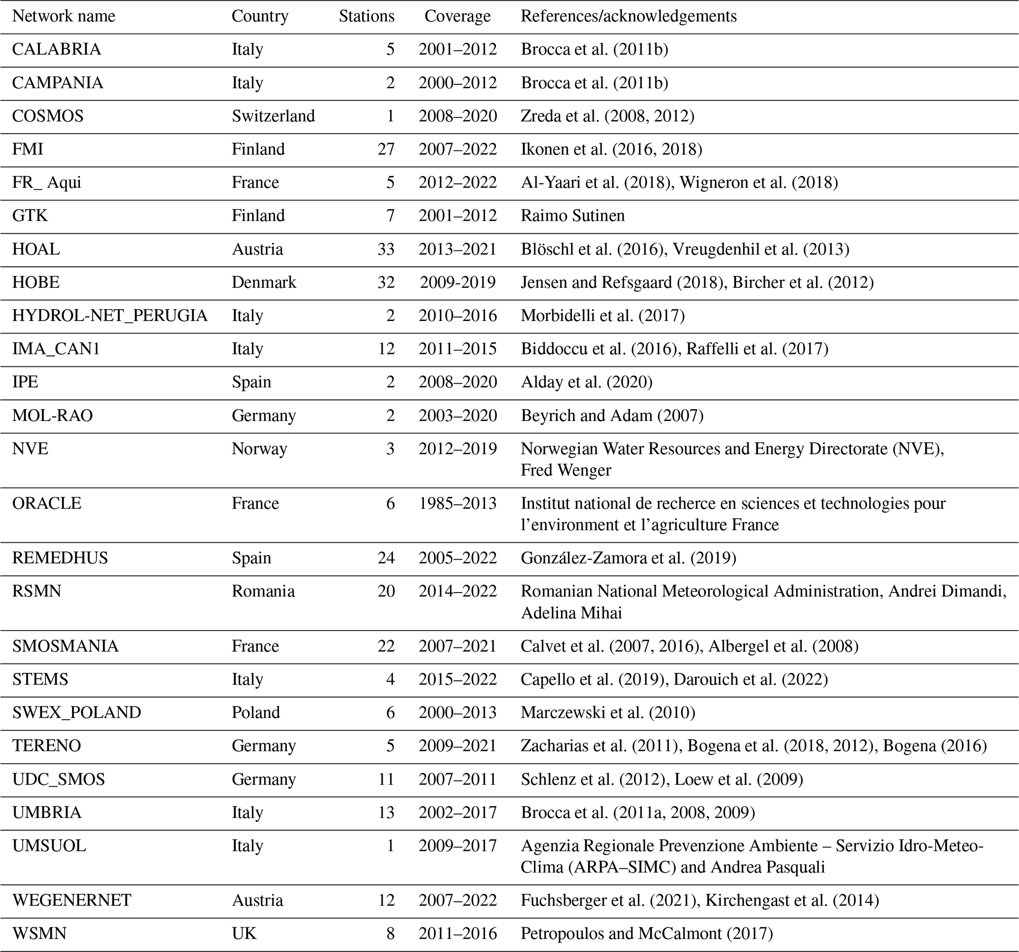
The International Soil Moisture Network (ISMN; Dorigo et al., 2021, 2011, 2013) provides in situ soil moisture data from over 70 soil moisture sensor networks around the globe. We calculated daily averages of in situ soil moisture data for depths of 0 cm to 10 cm (SM1) and 10 to 40 cm (SM2) from all networks providing station data within our modelling domain (see Table C1). Only data with quality flag of “good” were used, and we discarded stations with less than 1000 d of valid data within our evaluation period. Metrics were computed based on a nearest-neighbour matching between ISMN stations and model grid coordinates. In the case of multiple stations per model grid cell, we averaged the metrics of these stations to obtain a single value per model grid cell. Since soil moisture climatology and absolute values strongly depend on sub-grid scale factors like slope and soil texture, we only compared the in situ values in terms of the anomaly correlation R_anom. Additionally, we restricted the comparison to ISMN stations that have been shown to be representative at the 0.25^∘ resolution with a triple collocation analysis involving ISMN, ERA5-Land layer 1 SM, and ESA CCI SM (Dorigo et al., 2021, Fig. 7).

2.5.6 GRDC runoff

To evaluate the effects of the assimilation on modelled runoff, we used monthly river discharge station data from the Global Runoff Data Centre (GRDC; Koblenz, Germany). The station basins were derived from the provided watershed boundaries (GRDC, 2011).

The comparison of modelled total (surface + subsurface) runoff to station river discharge followed the approach of Koster et al. (2014, 2018), who compared river discharge with one basin-averaged runoff every 10 d. We restricted the analysis to 271 stations in Europe with a record of more than 10 years and a basin area between 625 and 100 000 km². The lower bound follows Kumar et al. (2014), while the upper bound was increased compared to Kumar et al. (2014) and Koster et al. (2018) in order to include more available stations in southern Europe (mainly Spain). We account for the larger area by using monthly averages instead of the average every 10 d that were used by Koster et al. (2018). Basins with a Pearson correlation of less than 0.4 with respect to the OL run were excluded so that the evaluation was not hampered by basins that are likely to be strongly affected by unmodelled processes (e.g. damming or irrigation).

2.5.7 Site data from Majadas

The ecosystem research site Majadas de Tiétar (Casals et al., 2009) is located in the center of the Iberian Peninsula at 39^∘56′25^′′ N 5^∘46^′29^′′ W and categorised as a semi-arid savanna type ecosystem (El-Madany et al., 2018) with a canopy height of 8.7±1.25 m and a fractional canopy cover of 23.0±5.3 % (Bogdanovich et al., 2021). In the land cover map used in the model, the grid cell containing the research site is classified as “savanna”. The accumulated annual precipitation at the site is about 650 mm, with large inter-annual variability. The mean LAI at the site changes strongly throughout the year, between 0.55–2.15 m² m⁻², with the lowest values occurring during summer and the highest values during late spring. The soil is an Abruptic Luvisol with a sandy upper layer (Nair et al., 2019). In the model, the grid cell containing the research site uses parameters for a loamy sand texture.

The research site consists of three eddy covariance towers with non-overlapping footprint climatologies and similar instrumental setups (El-Madany et al., 2021). For this analysis, the data from the tower with the FLUXNET ID ES-LM1 are used. A detailed description of the instrumental setup and data processing can be found in El-Madany et al. (2018, 2021). In short, the soil moisture data are collected with four profile probes (enviroSCAN, Sentek) measuring at 10, 20, 30, 50, and 100 cm plus an ML3 (Delta-T) sensor at 5 cm below the ground surface, but in close (unspecified) vicinity to the aforementioned profile probes. The soil moisture data were further aggregated to depth levels representing the Noah-MP soil moisture layers for each of the four profiles.

Eddy covariance data were collected at 20 Hz with a R3-50 (Gill) and a LI-7200 CO₂ and H₂O gas analyser (Licor Bioscience) at 15 m above the ground. Raw data were processed with EddyPro (Fratini and Mauder, 2014) to calculate fluxes of ET and CO₂ at half-hourly intervals. Subsequently, u^*-threshold estimation, gap filling, and flux partitioning were applied using REddyProc (Wutzler et al., 2018). The resulting continuous time series of ET and GPP were aggregated together with other meteorological parameters to hourly timestamps, from which daily averages were computed.

2.6 Analysis of Noah-MP equilibrium LAI

As will be seen later, each update step in the bias-blind DA is followed by a strong drift of the model LAI towards the earlier forecast values, i.e. the bias-blind DA system quickly “forgets” systematic corrections made in earlier steps. This indicates that there is a stable equilibrium LAI (i.e. a model-based “attractor”) whose value is not modified by the bias-blind LAI DA. To make full use of the information contained in the observations, a bias-blind DA system should also modify this equilibrium LAI value to have more persistent DA updates.

An analysis of the Noah-MP leaf growth model (Appendix A) shows that the main factors influencing the equilibrium LAI value are (i) root zone soil moisture, represented via the soil moisture factor β, and (ii) leaf parameters, e.g. specific leaf area (SLA, leaf mass per area). Including β or SLA in the DA state vector could thus help to obtain more persistent updates.

We therefore analysed how sensitive the equilibrium LAI is to these variables using a climatological approximation of the Noah-MP leaf model (shown in Appendix B). The result of this analysis is presented in Sect. 2.6 for two example sites with constrasting bias between Noah-MP and CGLS: (i) the Majadas site in Spain, where observed LAI is much lower than modelled LAI, and (ii) the Nile delta, where observed LAI is much higher than modelled LAI.

2.7 Evaluation of short-term DA effects

To evaluate how biased updates affect the short-term model performance, we analyse day-to-day differences of model states and fluxes. In the OL, the day-to-day differences are driven by day-to-day variations in the forcing. If averaged over larger areas or multiple years, this corresponds mainly to the fluctuations caused by the (long-term mean) seasonal cycle. For LAI, GPP, and ET, which are high in summer and low in winter, we therefore expect positive day-to-day differences in spring, corresponding to leaf growth and increases in GPP and ET, and negative day-to-day differences in autumn, corresponding to leaf shedding and decreases in GPP and ET.

Large update steps in the bias-blind DA can induce model instabilities. In this case, the subsequent day-to-day differences are strongly impacted by the unstable artificial response to the update step instead of reacting to the physical forcing input.

To detect if such model instabilities occur, and to what extent they propagate to flux estimates of the model, we evaluated differences in the estimates between day 2 and day 1 after assimilation as well between day 1 and day 2 before assimilation (the latter can also be interpreted as approximately day 9 minus day 8 after after assimilation). A comparison of these also gives an indication of how long the DA-induced effects persist. For each pixel and month, we calculated the median of these day-to-day differences over all years from 2003 to 2019 and normalised it with the monthly standard deviation of the variable values over the same multi-year time range (as a measure of the local within-month variation).

3 Results

3.1 Mean impact of bias-blind DA

Figure 1 compares mean values of OL and bias-blind DA results (relative to mean OL values) for different variables for the months of April through October across 17 years (2002–2019). The bias-blind DA decreases growing-season LAI over large parts of the domain or has a neutral impact. It only increases in the Alps and the Scandinavian Mountains. The regions with a large change in mean LAI are mostly semi-arid and include the Iberian Peninsula, northern Africa, the Middle East, Turkey, and Ukraine, where modelled LAI is much higher than observed LAI, and modelled LAI is therefore strongly decreased by the bias-blind DA. In contrast, LAI increases in the Nile delta, because the lack of irrigation forcing limits the model's ability to grow vegetation.

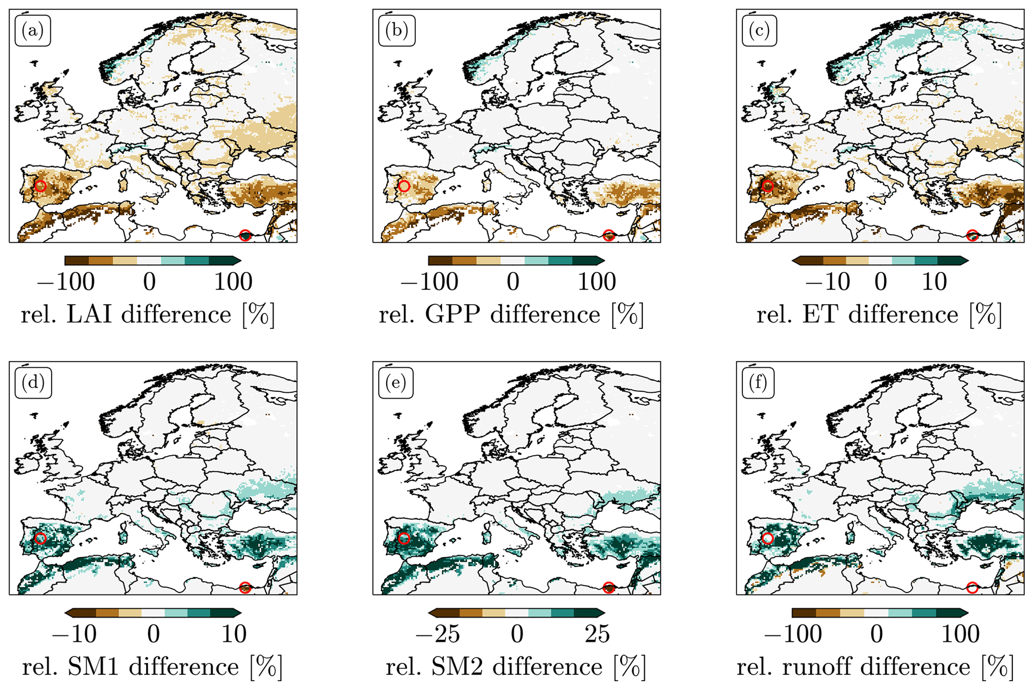
Figure 1 Relative differences between temporal mean values of the OL run and the bias-blind DA run for (a) LAI, (b) GPP, (c) ET, (d) SM1 (0–10 cm), (e) SM2 (10–40 cm), and (f) runoff for the months of April through October 2002–2019. Note the different colour bar ranges. The red circles mark the example locations studied in this work, i.e. Majadas in Spain and the Nile delta region in Egypt.

Differences in mean GPP show similar patterns, but with a weaker impact overall, especially in central and eastern Europe. One exception is the Nile delta, where growing-season GPP decreases while LAI increases. Relative differences in mean ET are much lower (note the different colour bar range), but with similar large-scale patterns to those for GPP. On the Iberian Peninsula, the patterns differ slightly: the largest relative differences are in the western part, mainly over the Duero and Tajo basins. Over Scandinavia, ET increases, except for the northernmost parts.

ET links the vegetation model to the hydrology model; consequently, the LAI assimilation also affects soil moisture and runoff. A reduction in LAI and hence transpiration leads to a reduction in soil moisture depletion. The effect is larger on deeper soil moisture layers than on surface soil moisture since the deeper layers are more strongly coupled with transpiration. In regions where LAI is strongly reduced by the DA, the relative increase in mean SM2 is about 20 %. For runoff, the relative increase even reaches 100 %. In contrast, in the Nile delta, the increase in LAI leads to a reduction in soil moisture via transpiration. In the Alps and Scandinavia, soil moisture is not affected systematically, since the water balance is dominated by runoff, and transpiration changes therefore have a lower impact.

3.2 Evaluation of the impacts of DA on GPP

The impacts of bias-blind LAI DA and bias-aware LAI DA on GPP are shown in Figs. 2 and 3, respectively. Bias-blind LAI DA strongly improves GPP estimates in terms of RMSD and R with FluxSat GPP and SIF (only R) over most of the domain, except in regions where the LAI bias is very large. In these regions, R with SIF degrades almost everywhere, and GPP RMSD and R with FluxSat degrades for some grid cells. The GPP R_anom with FluxSat improves in most areas, especially in those with large LAI biases. Similarly, the highest improvements in R_anom with SIF are found in areas with large LAI biases, excluding the Iberian Peninsula.

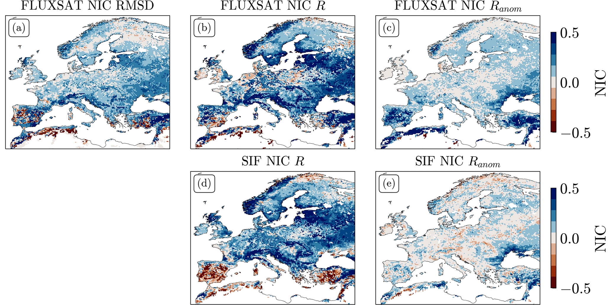
Figure 2 Maps of GPP NICs for the bias-blind DA for (a) RMSD with FluxSat, (b) R with FluxSat, (c) R_anom with FluxSat, (d) R with SIF, and (e) R_anom with SIF.

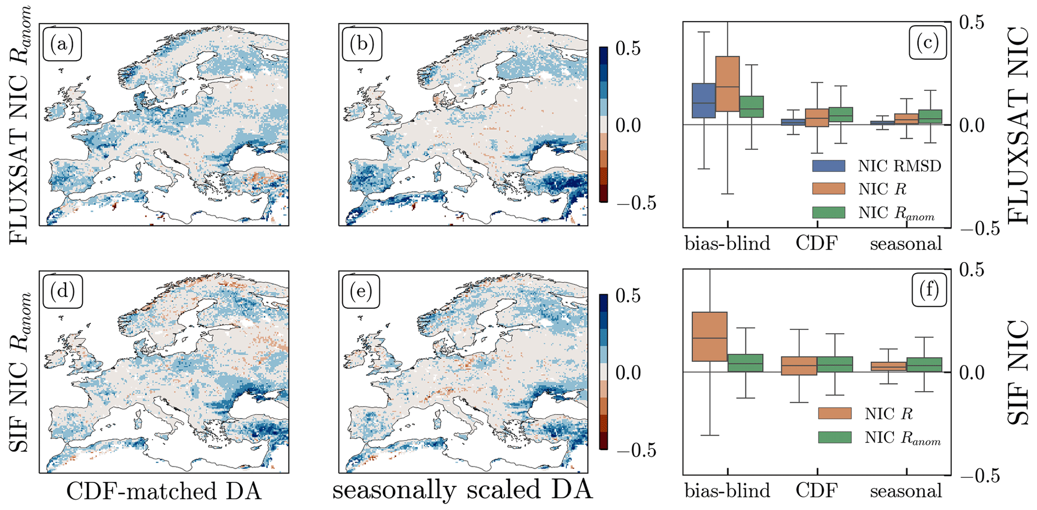
Figure 3 (a–c) Maps of NIC R_anom with FluxSat GPP for (a) the CDF-matched DA and (b) the seasonally scaled DA, and (c) box plots of NICs for RMSD, R, and R_anom with FluxSat GPP for all three DA runs. (d–f) Maps of NIC R_anom with SIF for (d) the CDF-matched DA and (e) the seasonally scaled DA, and (f) box plots of NICs for R and R_anom with SIF for all three DA runs. The upper limits of the box plots showing NIC R for the bias-blind DA (around 0.8 for FluxSat, 0.7 for SIF) have been cut to facilitate a better comparison with the bias-aware runs.

In the scaled LAI DA runs, the improvements in R_anom are similar, but the improvements in RMSD and R are lower, as summarised in Fig. 3c and f. The CDF-matched DA improves GPP R_anom with FluxSat over most regions, but not as strongly as the bias-blind DA (Fig. 3a) does. The seasonally scaled DA has largest improvements in regions with large LAI bias, where it outperforms the CDF-matched DA, and has a low impact over the rest of the domain (Fig. 3b). For SIF, the patterns of NIC R_anom are similar for all three runs (Fig. 3d and e).

3.3 Evaluation of the impacts of DA on hydrological variables

The impacts of bias-blind LAI DA and bias-aware LAI DA on hydrological ET and runoff fluxes are presented in Figs. 4 and 5, respectively.

.

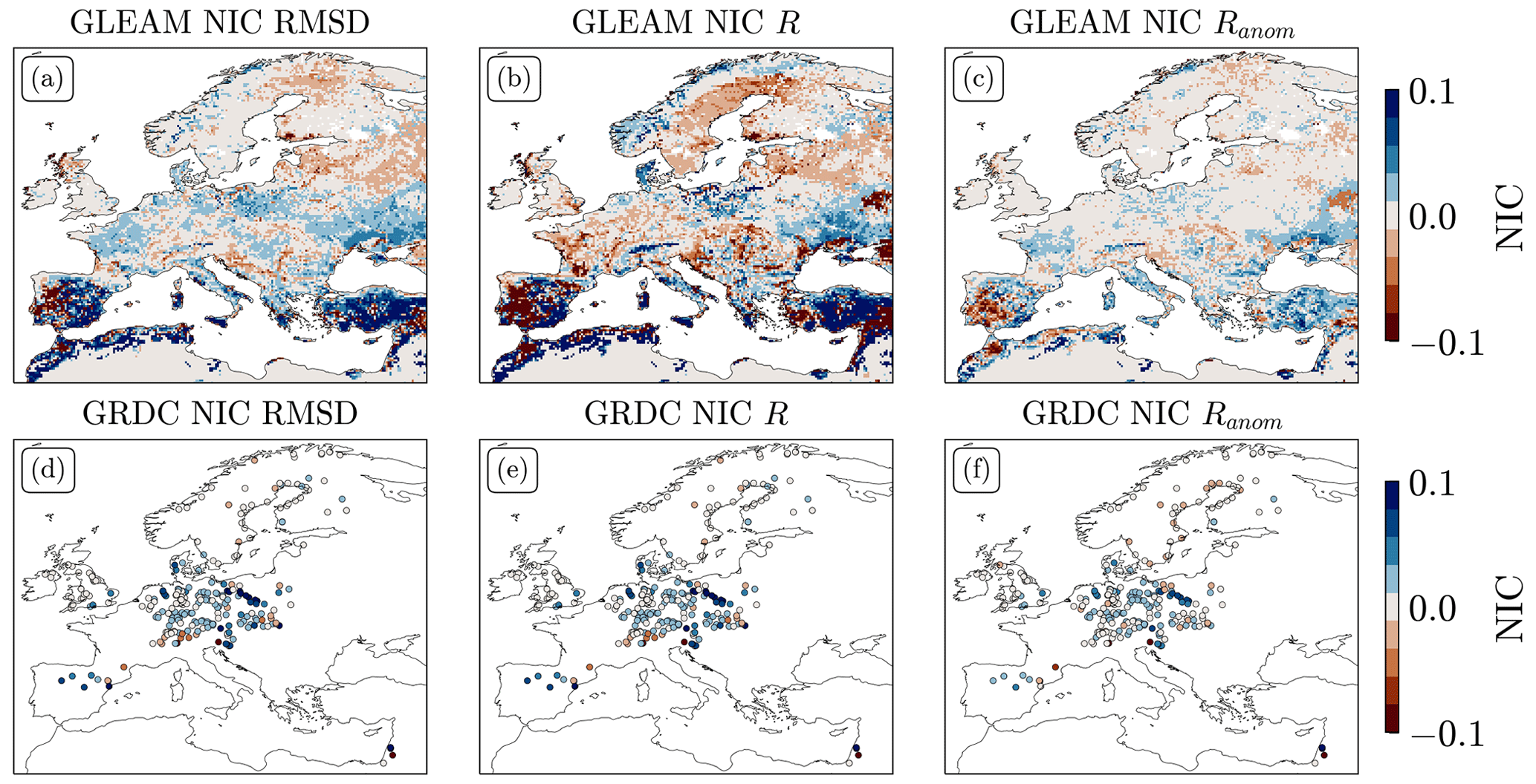
Figure 4 (a–c) Maps of ET NICs for the bias-blind DA for (a) RMSD with GLEAM, (b) R with GLEAM, and (c) R_anom with GLEAM. (d–f) Maps of runoff NICs for the bias-blind DA for (d) RMSD with GRDC, (e) R with GRDC, and (f) R_anom with GRDC. Note the different colour bar ranges compared to Fig. 2

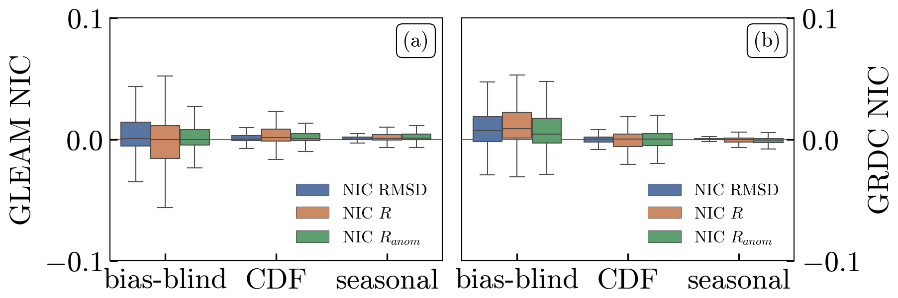
Figure 5 Box plots of RMSD, R, and R_anom NICs for all three DA runs with (a) GLEAM ET and (b) GRDC runoff.

The ET shows mixed results in terms of RMSD, R, and R_anom with GLEAM ET (Fig. 4a–c). The bias-blind DA improves the RMSD, R, and R_anom over most of Turkey and the eastern Iberian Peninsula, but degrades it over the western Iberian Peninsula and eastern Turkey. In central and eastern Europe, the RMSD improves over most agricultural regions, but R mostly degrades over these regions. In northern Europe, both the RMSD and R degrade compared to the OL run. The runoff estimates mainly improve in terms of RMSD, R, and R_anom with GRDC station data, especially in Spain and central Europe, but there is a negative impact in the Alps and Scandinavia (Fig. 4c–e). The rescaling techniques decrease both positive and negative DA impacts on ET and runoff, resulting in very low NICs (Fig. 5a and b).

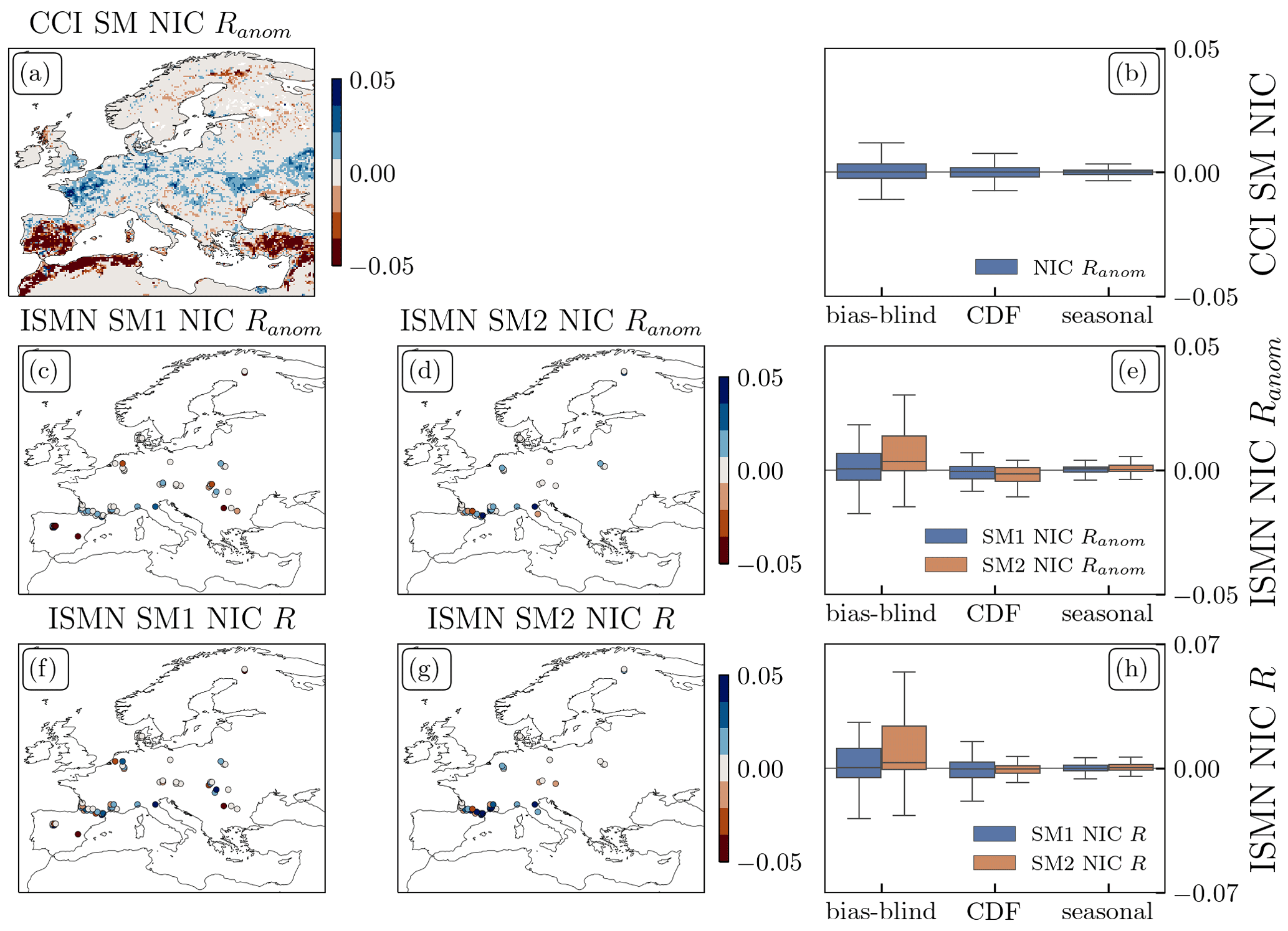
Figure 6 (a) Map of NIC R_anom with ESA CCI SM for the bias-blind DA and (b) box plots of NIC R_anom with ESA CCI SM for all three DA runs. (c–e) Maps of NIC R_anom with ISMN for the bias-blind DA for (c) SM1 (0–10 cm) R_anom and (d) SM2 (10–40 cm) R_anom, and (e) box plots of NIC R_anom with ISMN for SM1 and SM2 and all three DA runs. (f–h) Maps of NIC R with ISMN for the the bias-blind DA for (f) SM1 (0–10 cm) R and (g) SM2 (10–40 cm) R, and (h) box plots of NIC R with ISMN for SM1 and SM2 and all three DA runs. Note the different colour bar range compared to Figs. 2 and 4.

Finally, the DA results are evaluated in terms of surface (0–10 cm) and deeper (10–40 cm) soil moisture against in situ data and the ESA CCI SM in Fig. 6. The bias-blind DA leads to small improvements in deeper layer soil moisture in both R and R_anom, but none of the included ISMN stations are in the areas with large biases. The bias-aware DA does not affect metrics with ISMN significantly.

The comparison with the satellite-based ESA CCI SM presents a spatially more complete picture, with R_anom decreasing in regions with large LAI bias (Fig. 6d). R_anom also decreases over several mountain ranges and in Scandinavia but increases over agricultural areas in central Europe. The median NIC (Fig. 6e) is small for all experiments, with a smaller NIC spread for the rescaled DA runs.

3.4 Example I: Majadas site

To interpret the strong relative differences found in the previous section, we confront time series of multiple model variables with in situ data for the Majadas site in Fig. 7. We chose the years 2015 through 2017 as an example because of (1) the availability of in situ data, and (2) the considerable inter-annual variability in OL and observed LAI.

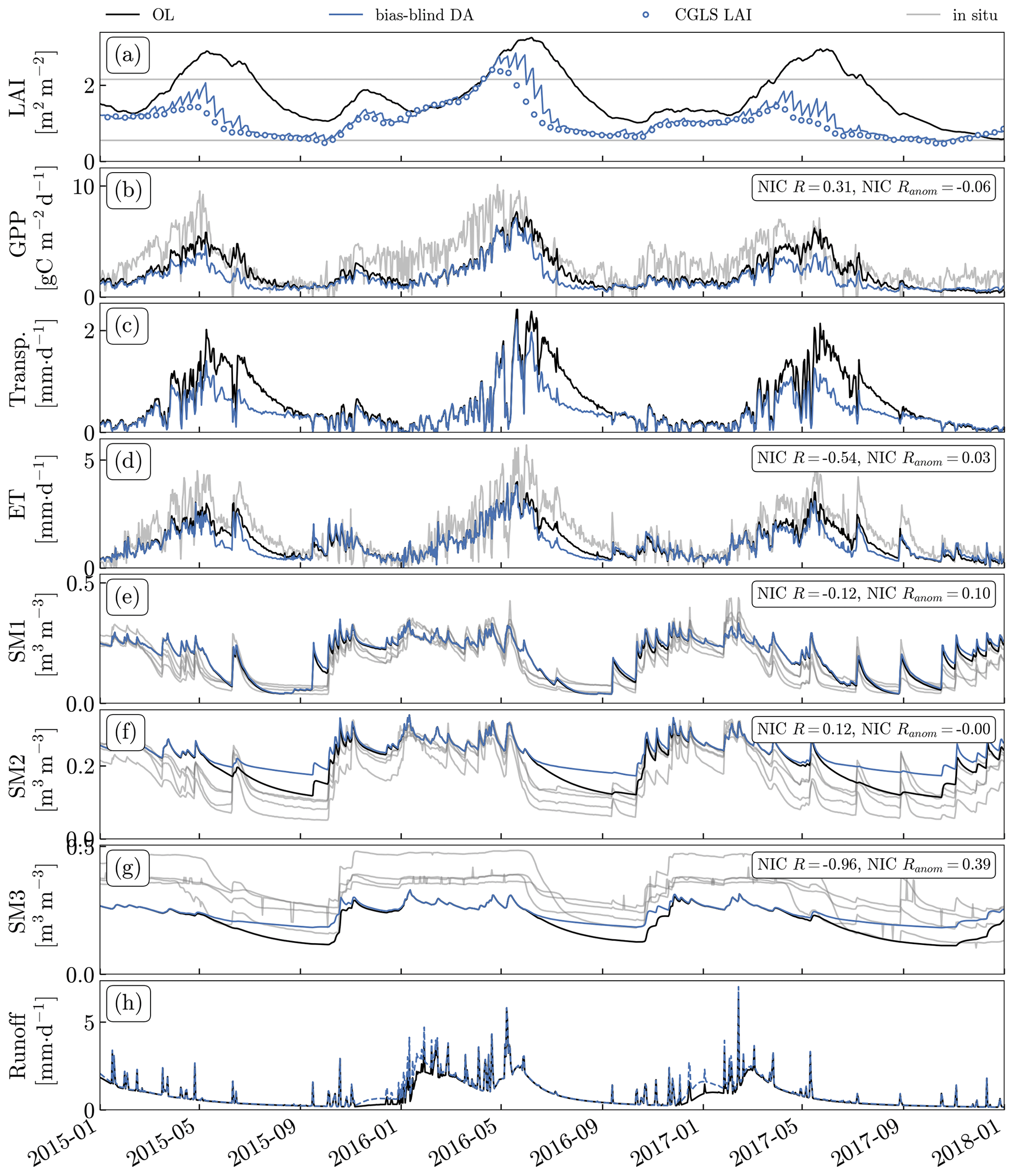
Figure 7 Time series of OL (black) and bias-blind DA (blue) results for (a) LAI, (b) GPP, (c) transpiration, (d) ET, (e) SM1 (0–10 cm), (f) SM2 (10–40 cm), (g) SM3 (40–100 cm), and (h) total runoff (surface + subsurface) for the model grid cell containing the Majadas site (39.875, −5.875^∘). Panel (a) also shows the assimilated LAI observations (blue dots) and the minimum and maximum observed LAI at the site (grey lines). For the other panels, in situ data from the Majadas site are also shown (grey lines), if available, and the NICs for R and R_anom (calculated based on the full period of data availability) are indicated in the panels.

The OL and CGLS LAI show some similar features in their temporal patterns, but the timing and magnitude disagree. Both show peaks in late spring or summer and reach their minimum in early autumn, followed by a small increase (Fig. 7a). They also agree that the peak in spring/summer 2016 is the highest among these 3 years. However, the CGLS LAI reaches its maximum by the start of May and then rapidly decreases, while the OL reaches its maximum later and decreases more slowly. Additionally, the OL has a higher overall LAI and a lower inter-annual variation in the maximum peak than the CGLS LAI. The magnitudes of the spring maxima and the summer minima also match the observed maximum and minimum values better (2.15 and 0.55 m² m⁻²: lower and upper thick grey lines in Fig. 7a, respectively). The large differences in summer lead to pronounced sawtooth patterns in the bias-blind DA results, showing that the model undergoes a strong drift back towards the equilibrium state after each DA update.

The decrease in summer LAI in the DA also induces a decrease in summer GPP (Fig. 7b). This increases R with the in situ flux tower measurements, but slightly decreases R_anom. A better agreement can be seen in spring 2015, where observed and analysed GPP decline faster than the OL, and in spring 2017, where the OL GPP increases until mid May, while DA and observations stay at the same level as in April. The differences in overall magnitude between the in situ data and the model might be caused by representativeness errors; for example, differences in the assumed canopy cover for the savanna land cover class in the model and the canopy cover at the Majadas site.

Transpiration strongly decreases in summer as a consequence of the lower LAI (Fig. 7c), which leads to a lower ET (Fig. 7d). For the latter, correlation with the in situ data decreases, in agreement with the decreased correlation with GLEAM ET in the western Iberian Peninsula seen in Fig. 4a, while the anomaly correlation slightly increases.

Soil moisture also increases, with a larger effect in the deeper layers (Fig. 7e–g). The first layer (0–10 cm) is only slightly affected, but the deeper layers (layer 2 = 10–40 cm, layer 3 = 40–100 cm, layer 4 = 100–200 cm (not shown)) are much wetter in summer and autumn, caused by a slower drying rate. These large changes are hard to compare across scales since the soil moisture climatology depends strongly on local factors like soil texture or topography (Dong and Ochsner, 2018).

The changes in the model LAI also affect surface and subsurface runoff (Fig. 7h). The main difference in the example grid cell is an increased subsurface runoff for the analysis in winter 2016 and 2017.

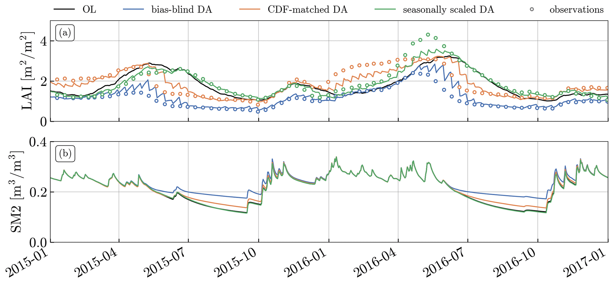
Figure 8 Time series of (a) LAI and (b) SM2 (10–40 cm) for all DA runs for the Majadas grid cell. Panel (a) includes the (potentially rescaled) observations that were assimilated in each run (coloured dots; dot colours correspond to line colours).

Figure 8 shows that the two rescaling techniques studied in this paper reduce the difference between OL and analysis LAI. In the CDF-matched DA, winter LAI is higher than in the OL, while autumn LAI drops faster than in the OL. This leads to differences in layer 2 soil moisture in autumn, although they are not as strong as in the bias-blind DA. The seasonally scaled DA follows the OL more closely. The rescaled runs still contain the sawtooth pattern that was present in Fig. 7a, but often with a less steep drift between updates and with seasonally varying directions. Seasonal rescaling is especially good at reducing the sawtooth pattern.

3.5 Example II: Nile delta

As another example, we examined the Nile delta, where observed LAI strongly exceeds OL LAI, but summer GPP in the DA results strongly decreases compared to the OL (see Fig. 1). The low vegetation in the OL is caused by a lack of irrigation in the model, which results in water limitations on vegetation growth. Figure 9a shows that the bias-blind DA strongly increases LAI, causing it to follow the observations more closely. However, it also strongly decreases SM2 (Fig. 9b), such that the wettest conditions in the bias-blind DA are still drier than the driest conditions in the OL. As a consequence, SM2 falls below the model wilting point in summer, and the model disables photosynthesis due to water stress (Fig. 9c). This decouples analysed LAI and GPP in summer and explains the decrease in April to October GPP seen in Fig. 1. Instead of correcting the root cause of the LAI underestimation, the bias-blind DA worsens the problem here.

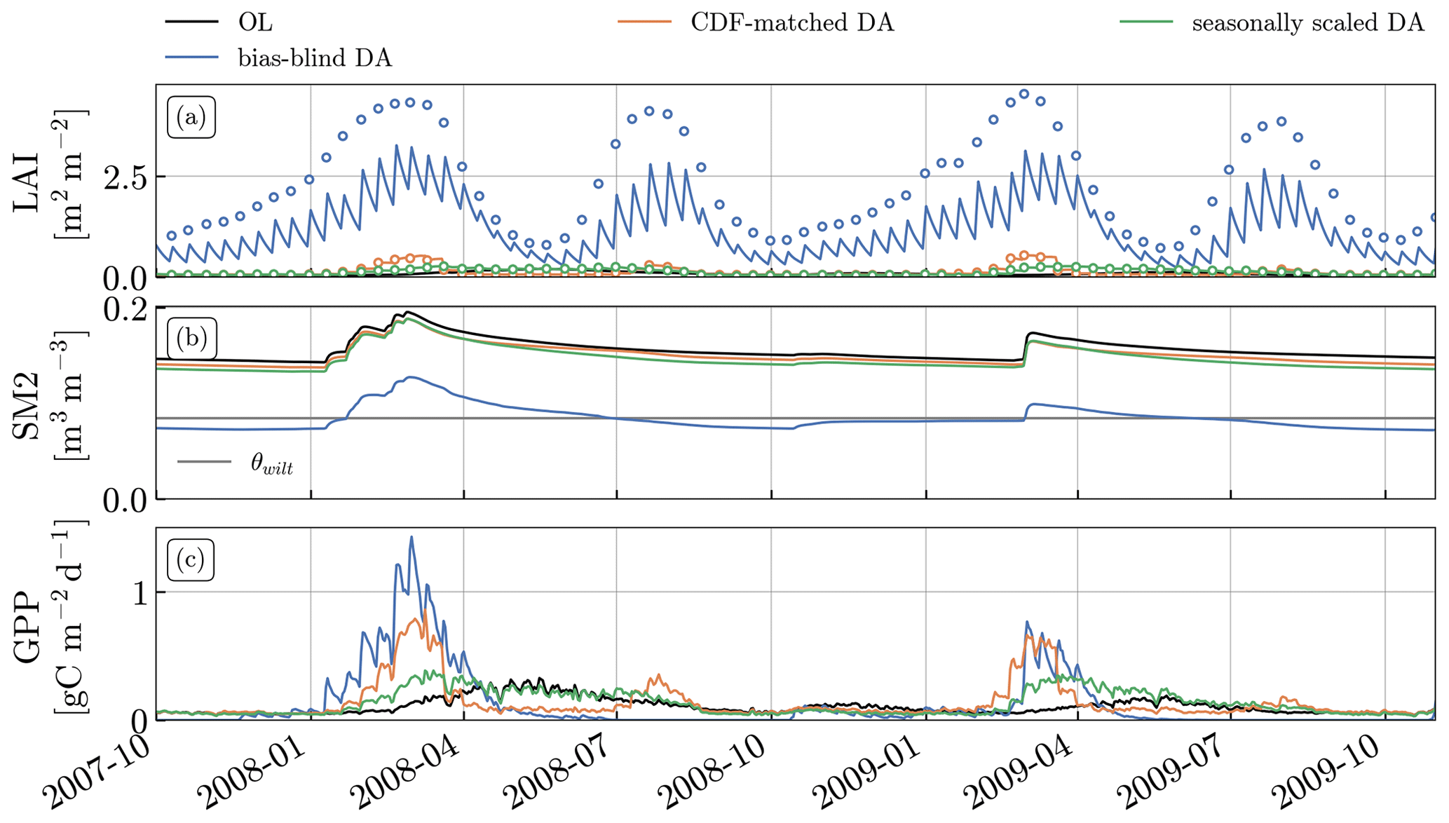
Figure 9 Time series of (a) LAI, (b) SM2 (10–40 cm), and (c) GPP for all DA runs for the Nile delta example grid cell (31.125, 30.875^∘). Panel (a) includes the (potentially rescaled) observations that were assimilated in each run (coloured dots; dot colours correspond to line colours).

3.6 Analysis of equilibrium LAI

We assessed the dependency of the equilibrium LAI value on the model root-zone soil moisture (via the relative amount of plant-available water β) and on model parameters (using the specific leaf area, SLA, as an example parameter) for the two example sites discussed above.

Figure 10 shows how the equilibrium LAI changes when we change β or SLA while keeping everything else constant. For both of the sites shown (Majadas, the Nile delta), we chose the month where the mean difference between OL and observations is largest (June for Majadas, July for the Nile delta). We approximated the GPP–LAI relationship for these sites and months based on Eq. (B1).

Figure 10 Estimates of the rate of change in LAI ($\mathrm{dLAI}/\mathrm{d}t$) for the Noah-MP LAI and equilibrium LAI for the Majadas pixel in June (a, b) and the Nile delta pixel in July (c, d) as a function of the relative amount of plant-available water β (a, c) and specific leaf area (SLA, b, d). Additionally, the mean conditions for the OL and the DA runs are shown as symbols (dots, crosses), and the mean assimilated CGLS LAI is shown as a red line.

For both of the cases considered, the mean OL conditions are close to the estimated equilibrium LAI, validating the approximations we used in the derivation of the method (Sect. 2.6). For Majadas, the mean June conditions of the seasonally scaled DA are very close to the OL, while the bias-blind DA shows a strongly reduced LAI and an increased β, consistent with Fig. 8. The CDF-matched DA is between the OL and bias-blind DA. Both the bias-blind and CDF-matched DA are further from the estimated equilibrium LAI than the seasonally scaled DA, i.e. they are not in a stable state. To obtain a stable state but at the same time reduce LAI towards the CGLS LAI observations, β would have to be reduced to about 0.3 or, alternatively, SLA would have to be reduced to 30.

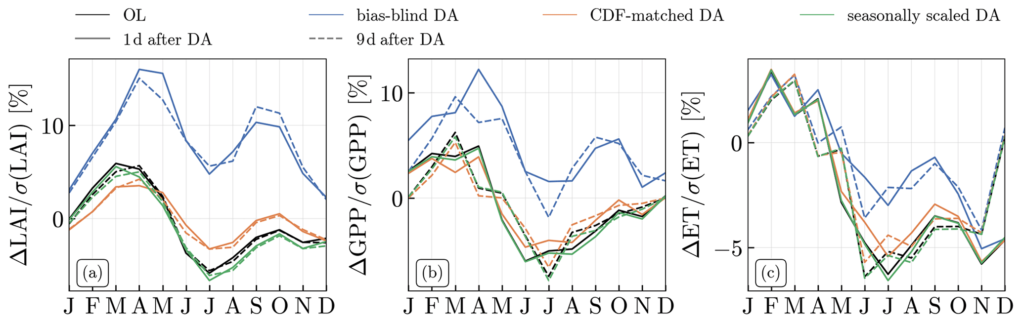
Figure 11 Normalised monthly median day-to-day forecast differences for (a) LAI, (b) GPP, and (c) ET. The differences are computed as the forecast value at 2 d after observations minus that at 1 d after observations (“1 d after DA”, solid lines) and the forecast value at 1 d before observations minus that at 2 d before observations, corresponding to approximately 9 d after observations minus 8 d after observations (“9 d after DA”, dashed lines) for the OL (black), the bias-blind DA (blue), the CDF-matched DA (orange), and the seasonally scaled DA (green). The median was calculated from all grid cells for which the relative LAI difference between OL and bias-blind DA (see Fig. 1a) is below −25 %. For each grid cell and month, the median was normalised with the monthly standard deviation of the variable for this grid cell. The graph shows the median results across 17 years (2003–2019).

For the Nile delta pixel, both bias-aware DA runs are very close to the OL, while the bias-blind DA shows a strongly reduced β, consistent with summer conditions in Fig. 9. In this pixel, the equilibrium LAI shows a much higher sensitivity to β; a small increase in β leads to a large increase in LAI. Conversely, the sensitivity to SLA is low. To obtain a stable state close to the observed LAI, β would have to be increased to 0.5, while SLA would have to be increased to values larger than 150.

3.7 Evaluation of short-term DA effects

Figure 11 shows the monthly median day-to-day forecast differences for all simulation runs performed for LAI, GPP, and ET. The OL shows a seasonal cycle with high values in spring and low values in summer, as expected (corresponding to the derivative of the seasonal cycle of variable values). The bias-aware DA runs closely follow the OL seasonal cycle.

The bias-blind DA also shows the same seasonal cycle, but it has an offset compared to the OL. For LAI, this offset is of the same size as the magnitude of the mean seasonal cycle, so that the mean day-to-day differences in the bias-blind DA in summer have the same magnitude as the day-to-day differences in the OL in spring, even though a decrease in LAI is expected physically. In fact, the day-to-day differences in LAI in the bias-blind DA are always positive, meaning that LAI is expected to increase in all seasons. This is caused by the large DA update steps in the bias-blind DA, which pull the model to an unstable state. As a consequence, model instability instead of physical forcing input governs the short-term temporal evolution of LAI in the model in between update steps. Even 9 d after the DA update, right before the next update step, day-to-day differences do not significantly change, indicating that the model instability can persist for long time periods.

The instability effect also strongly affects GPP estimates throughout all seasons and, to a lesser extent, ET estimates in summer.

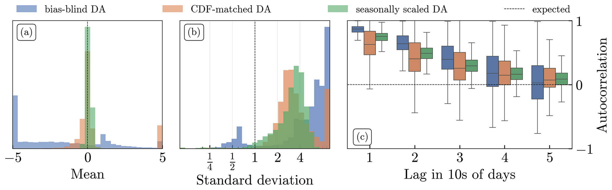
Figure 12 Spatial distributions of the temporal (a) mean, (b) standard deviation, and (c) autocorrelation of the innovations across all model grid cells. In panels (a, b), values for means and standard deviations outside the plot ranges of the histograms have been added to the first and last bin, respectively. In panel (c), the autocorrelation is computed for multiple lags of 10 d.

3.8 DA diagnostics

Figure 12 shows distributions of innovation statistics across the modelling domain and shows that the innovation sequence is not standard normal for the bias-blind DA. As a consequence of the higher LAI in the model, the normalised innovation mean is strongly negative (Fig. 12a), and the absolute values of the innovations are large (Fig. 12b). The autocorrelation is also high (Fig. 12c) because subsequent updates point in the same direction.

The rescaling improves the internal diagnostics of the DA system. Although there is still a sawtooth pattern (Fig. 8), the assumption of zero mean innovations is met, and rescaling helps to reduce the innovation variance (Fig. 12b) and the autocorrelation (Fig. 12c) compared to the bias-blind DA run.

4 Discussion

4.1 General impacts of bias-blind and bias-aware DA

Our analysis shows that large biases between Noah-MP modelled LAI and CGLS LAI exist. These include a bias in the length of the growing season, which might be caused by processes not included in the model (e.g. agriculture) or biased forcing data, but also by a strong bias in the CGLS LAI magnitude. It is most pronounced over dry areas in the southern part of the modelling domain, in line with results from Li et al. (2022), who also found an overestimation of LAI by Noah-MP's dynamic vegetation model with respect to MODIS LAI in this area. Noah-MP is not unique in this respect; studies with other LSMs have also found model deficiencies in dry regions (Dahlin et al., 2015; MacBean et al., 2015; Fox et al., 2018; Mahmud et al., 2021).

The bias-blind LAI DA therefore has a strong impact on the vegetation model state and fluxes. Where the LAI bias is large, the bias-blind DA induces strong changes in GPP magnitude, which mostly reduce the RMSD with FluxSat, in agreement with results found by Kumar et al. (2019b) and Albergel et al. (2020) for similar GPP reference datasets. The anomaly correlation improvement differs for FluxSat and SIF, but both show a generally positive impact. The difference might be due to the dependence of both the assimilated LAI observations and the FluxSat GPP retrievals on reflectances from optical satellite sensors, which might inflate anomaly correlations.

The strong impacts of the bias-blind DA also propagate to the model hydrology. Results for ET estimates are mixed: RMSD and R_anom with GLEAM generally improve, especially over Turkey, the western Iberian Peninsula, and agricultural regions, but R deteriorates over most of the domain. In contrast, runoff estimates improve compared to the GRDC discharge data. The comparison to ISMN indicates improvements in deeper layer soil moisture, but none of the in situ sites considered are in the areas with a large bias. The anomaly correlation with ESA CCI SM also improves over agricultural regions but decreases over high-bias regions and northeastern Europe. However, in northeastern Europe, the Noah-MP model-only SM estimates outperform ESA CCI SM when comparing to in situ sites (Heyvaert et al., 2023), probably due to the lower signal-to-noise ratio of soil moisture retrievals over dense vegetation (Gruber et al., 2019).

The large changes to the root-zone soil moisture climatology are hard to assess directly because of the scale difference between the in situ data and model grid cells and the lack of in situ sites in these areas. However, in strongly irrigated areas, the change in soil moisture climatology leads to a decrease in soil moisture, even though the bad model performance originates from an underestimation of soil moisture due to the lack of an irrigation process in the model. Joint updates of LAI and root-zone soil moisture, as done in LDAS-Monde (Albergel et al., 2017), could alleviate this problem caused by “missing” water to some extent, but they require a good estimation of the coupling strength of LAI and soil moisture. The strong effect on the model hydrology might also be model specific, because the Noah-MP model hydrology is more sensitive to vegetation than other LSMs (Maertens et al., 2021).

Even though our results for RMSD improvements in GPP and ET are similar to those from other studies (Kumar et al., 2019b; Albergel et al., 2020), it is important to note that none of the reference products we used are free of bias. This could be due to assumptions and errors in the underlying satellite data and retrieval algorithms in the case of satellite-based data, or due to different spatial support in the case of in situ data. Hence, whether the bias-blind DA leads to estimates closer to the “truth” remains uncertain, and evaluations with different reference products might come to different conclusions. We therefore additionally investigated effects of the DA on the model and on internal DA diagnostics.

4.2 Negative effects on the optimality of the DA system when ignoring bias

An effect of “misusing” a Kalman filter for correcting biases instead of random errors is that DA updates are strongly biased, leading to non-optimal DA diagnostics and a pronounced sawtooth pattern. Such sawtooth patterns are common in filter DA (e.g. Mitchell et al., 2002; Dee, 2005; Fox et al., 2018), but the strong preference for one direction and the model drift between two update steps harms estimates of other variables. GPP and ET are strongly reduced at the time of the DA update, and the short-term model forecasts directly after the DA update step show unphysical upward drifts.

The sawtooth pattern also poses the danger of introducing spurious trends in case the observation frequency changes over time (Dee, 2005). For example, if the availability of LAI observations at the Majadas site increased over time, the model would be pulled more closely to the observations, i.e. there would be lower LAI values in the later periods than in the early period, leading to an apparent decrease in LAI. Due to the strong impact of LAI changes on soil moisture, this would also lead to a spurious wetting trend in the deeper soil layers. Such artificial trends can seriously confound trends in the resulting dataset.

The sawtooth pattern has also been reported by other LAI DA studies using Noah-MP (Kumar et al., 2019b; Mocko et al., 2021). We showed that the Noah-MP leaf model structure has an equilibrium LAI (independent of the current model state) to which the model tries to return after each update step. Bias-blind LAI DA into LSMs with a similar model structure might therefore suffer from the similar issues.

The sawtooth pattern can be reduced by interpolating the observations or by applying time series smoothing methods to obtain pseudo-observations at a daily frequency. This will keep the analysis closer to the observations and prevent model drift over multiple days. However, in this case, direct insertion approaches or using observed LAI directly as a model parameter could achieve even better results than an EnKF at a much lower computational cost.

4.3 Effects of bias-aware DA

Using rescaling techniques for a priori bias correction comes at the cost of foregoing improvements in ET, runoff, and GPP. However, the rescaling techniques retain improvements in GPP anomaly correlation and limit the side effects of the LAI DA on model hydrology. The CDF matching performs better for GPP anomalies over central Europe and for ET over the high-bias regions since it preserves more information on the shape of the observed seasonal cycle of LAI. But, due to its larger impact on ET compared to seasonal rescaling, it also changes the soil moisture climatology in deeper layers and leads to a decrease in anomaly correlation with in situ soil moisture, especially for deeper layers. The seasonal rescaling presents better performance for GPP anomalies over the high-bias regions when using FluxSat GPP as reference, but not with SIF, which may indicate an overestimation of skill, as discussed above. Overall, the seasonal rescaling minimises the effects of DA on the model hydrology.

Since the bias-aware DA only allows the DA to address the random error components, filter diagnostics are more in line with standard assumptions (Desroziers et al., 2005). This facilitates a further reduction in the variance and autocorrelation of the normalised innovations to obtain an optimal filter configuration by tuning the model and observation perturbations.

The limited DA impacts and more well-behaved filter performance could be especially helpful when assimilating multiple datasets, because contrasting biases could deteriorate the ability of the DA system to find a good compromise between multiple observations and model predictions (MacBean et al., 2016). This might, for example, arise if variables that require more complex observation operators are assimilated and the observation operator is calibrated to the original model climatology.

4.4 Alternatives to the rescaling of observations

The bias-aware DA uses observation rescaling methods to reduce the effects of biased updates like drifts and sawtooth patterns, but it leads to lower improvements than the bias-blind DA because it leads to LAI estimates in the model climatology. To obtain LAI estimates within the range of the observational LAI climatology while keeping the model in a stable state, additional model state variables or parameters have to be updated or calibrated, or an observation or forecast bias could be estimated separately (and removed from the innovations) (De Lannoy et al., 2007a, b).

The calibration of model parameters is the best option if the bias is due to uncertainty in the model parameters. It has been successful at improving vegetation models in previous studies (MacBean et al., 2015, 2016; Scholze et al., 2019; Forkel et al., 2019; Kolassa et al., 2020; Mahmud et al., 2021). Updates of the specific leaf area together with LAI have already been used successfully by Xu et al. (2021) and He et al. (2022). Based on Eq. (A1), changes in the leaf turnover coefficient or the respiration coefficient might lead to similar results.

The calibration can either be done prior to the DA simulations or it can be incorporated into a joint parameter and state update DA scheme. An EnKF (such as that used in this study) can in principle be used for the joint updates by augmenting the control vector to contain both state variables and parameters (Evensen, 2009). If the model predictions' dependency on the parameters is highly nonlinear, particle methods might be more suitable (Frei and Künsch, 2013; van Leeuwen et al., 2019). Hybrid methods that combine the EnKF with particle methods could be used to obtain a DA system that performs well both for state updates and parameter updates (Frei and Künsch, 2013; van Leeuwen et al., 2019; De Lannoy et al., 2022).

Instead, if the (short-term) bias is caused by erroneous forcing data, e.g. a seasonal wet or dry bias in water-limited areas, joint updates of LAI and RZSM (root-zone soil moisture) are better suited to improving the analysis. This is the approach chosen for (bias-blind) LAI DA in LDAS-Monde (Albergel et al., 2017). With an EnKF, joint updates are achieved via error cross-correlations between LAI and RZSM (obtained from the ensemble). This means that RZSM will only be updated in phases in which model LAI and RZSM show a strong coupling.

A known source of bias in the Nile delta is the missing irrigation input in the model. Additionally, we found a very strong water limitation on vegetation growth and a strong sensitivity of the equilibrium LAI to changes in RZSM, implying a strong model coupling of LAI and RZSM. Therefore, joint updates of LAI and RZSM are likely to improve the LAI DA results here because RZSM is temporarily adjusted, but changes to soil parameters might also be necessary to sustain the increased moisture values.

At the Majadas site, the sensitivity of the equilibrium LAI to changes in RZSM is lower. Furthermore, Fig. 8 indicates that in winter and spring, RZSM is largely dominated by soil parameters and precipitation input. In these periods, changes in LAI do not lead to changes in RZSM, and differences in RZSM between the OL and the bias-blind DA vanish quickly. Therefore, RZSM updates are unlikely to sustainably decrease RZSM during spring, which would be required to decrease LAI to a more stable state. This could make joint updates of LAI and RZSM less efficient than in the Nile delta. Parameter updates are likely most useful for improving the LAI estimates at the Majadas site.

4.5 Potential model structural changes

The vegetation model in Noah-MP consists of two parts: a photosynthesis model, which calculates how much carbon is assimilated from the atmosphere in each time step, and the dynamic vegetation model, which distributes the carbon to different plant carbon pools and calculates losses due to respiration and turnover. Previous studies found that the dynamic leaf model decreases performance compared to a prescribed LAI (Ma et al., 2017; Erlingis et al., 2021; Huang et al., 2022). Structural changes to the equations governing the leaf carbon assimilation might therefore improve the agreement between modelled and observed LAI.

A promising candidate for structural changes is the leaf carbon allocation function, which governs the fraction of the photosynthesis carbon that is allocated to the leaves. In Noah-MP v4.0.1, this function decreases from 1 at LAI = 0 to 0 at approximately LAI = 6 with a sigmoid-like shape. Alternative formulations have been tested by Gim et al. (2017) and Niu et al. (2020). They used sigmoidal functions with a sharp decline around a threshold LAI. This would increase the model drift towards the equilibrium (the threshold LAI) and therefore likely worsen the instability in a bias-blind DA setup. But, when treating this threshold as a model parameter, these formulations open up new possibilities for calibration and parameter data assimilation, since the threshold LAI gives a more direct route to adapting the maximum LAI reached in summer. Multi-pass schemes that update the threshold based on observations, similar to Xu et al. (2021), might be able to improve the persistence of observations and alleviate the sawtooth pattern issue.

Another shortcoming of Noah-MP is its oversimplified phenology scheme, which is solely based on a land-cover-specific canopy temperature threshold, ignoring other drivers of phenology like day length or water availability (e.g. Dahlin et al., 2015, 2017) or cumulative temperature effects that are often expressed via growing degree days (e.g. in CLM, Lawrence et al., 2011). Especially in the southern part of our modelling domain, where water partly limits vegetation growth (Hashimoto et al., 2019), more complex phenology schemes might improve the realism of the vegetation simulations. In the current scheme, the temperature threshold is almost always exceeded, leading to unrealistically long growing seasons. However, additional degrees of freedom introduced by a more complex phenology scheme can also deteriorate model predictions (Lawrence et al., 2011).

5 Conclusions

So far, satellite LAI DA studies have mostly ignored biases between observed and modelled LAI. In this study, we evaluated how the presence of bias in an LAI DA system can impact the model hydrology and carbon uptake. Specifically, we assimilated CGLS LAI into Noah-MP with an EnKF, and we evaluated a bias-blind DA and two rescaling techniques, i.e. climatological CDF matching and seasonal rescaling of the first two moments, to account for the biases in the DA system.

The bias-blind DA is most effective at reducing the disagreement between modelled and observed LAI, and leads to the largest improvements in GPP and runoff. It is therefore a suitable option for many applications, especially if large bias reductions are intended, even though bias-blind Kalman filtering is suboptimal. A temporal interpolation of the observation data, or even a direct insertion approach, could be even more efficient for such a purpose. However, this approach does not necessarily improve other variables, e.g. if the model simulates biased LAI in conjunction with unbiased soil moisture. As an alternative, we recommend using observation rescaling techniques for LAI DA with Noah-MP if there are strong biases and if

• the focus is on not only vegetation or the carbon cycle but also hydrological processes, because large LAI changes can cause unphysical impacts on the model hydrology;

• multiple datasets with contrasting biases are assimilated, since the bias-blind DA can strongly change the model climatology;

• the DA aims at preparing the best analysis state for subsequent short-term predictions, because the abrupt update steps induce spurious short-term trends;

• datasets with changes in observation frequency are used, because this can induce spurious long-term trends;

• an optimal DA system in terms of Desroziers' metrics (Desroziers et al., 2005) is desired, because bias-blind DA violates basic assumptions of the Kalman filter.

The CDF-matching technique preserves more information from the signal and leads to larger improvements in GPP and ET but worse estimates of deeper layer soil moisture. The seasonal rescaling is more effective at removing bias and limits DA updates to improve vegetation anomalies; it performs best in terms of internal DA diagnostics. The bias-aware LAI DA is suitable for providing physically consistent short-term flux estimates for numerical weather prediction models or soil moisture monitoring or for providing a baseline to merge historical earth observation records from multiple sensors into a long-term dataset without introducing artificial trends.

A drawback of the observation rescaling approaches is that they result in estimates in the model climatology. If the observation–forecast bias is due to erroneous precipitation forcing or missing irrigation input, joint updates of LAI and RZSM in a bias-blind system can be considered instead. This might lead to large bias corrections while still retaining a stable model state even after large updates. However, if the bias is not only caused by bias in the precipitation/irrigation, this poses the risk of seriously degrading the soil moisture estimates.

Alternatively, updates to model parameters, either via joint parameter and state update DA or via a priori model calibration, can also lead to more stable and persistent updates and LAI estimates in the observational climatology. This is especially desirable for research on the carbon cycle, where absolute values of carbon fluxes are required. Parameters to consider for calibration are parameters related to model leaf growth, but potentially also photosynthesis or soil parameters.

To gain the most benefit from LAI data assimilation into Noah-MP, further research and improvement in the modelling of the coupling mechanisms between the water and carbon cycle is necessary.

Appendix A: Noah-MP dynamic leaf model

This section gives a short overview of the Noah-MP vegetation model, focusing on the interaction of LAI and soil moisture. For a more detailed description, we refer the reader to Niu et al. (2011).

Noah-MP calculates LAI from a prognostic leaf biomass C_l and a vegetation-type specific leaf area per leaf mass (specific leaf area; SLA):

$$\mathrm{LAI}=\mathrm{SLA}\cdot C_{\mathrm{l}}.$$

Leaf biomass is updated in each step via a mass balance equation:

$$\begin{array}{}\text{(A1)}& \begin{array}{rl}{\displaystyle \frac{\mathrm{d}{C}_{\mathrm{l}}}{\mathrm{d}t}}& ={\displaystyle \frac{\mathrm{1}}{\mathrm{SLA}}}{\displaystyle \frac{\mathrm{d}\mathrm{LAI}}{\mathrm{d}t}}=(\mathrm{1}-\mathrm{FRAGR})\\ & \cdot \left[f_{\mathrm{l}}\left(\mathrm{LAI}\right)\cdot \mathrm{GPP}\left(\mathrm{LAI},\mathit{\beta },T_{\mathrm{c}},F\right)-R_{\mathrm{m}}\left(\mathrm{LAI},\mathit{\beta },T_{\mathrm{c}}\right)\right]\\ & -D_{\mathrm{c}}\left(\mathrm{LAI},T_{\mathrm{c}}\right)-D_{\mathrm{d}}(\mathrm{LAI},\mathit{\beta })-T_{\mathrm{l}}\left(\mathrm{LAI}\right),\end{array}\end{array}$$

with FRAGR the fraction of GPP minus maintenance respiration invested in growth respiration, R_m the maintenance respiration, D_c the death rate due to cold stress, D_d the death rate due to drought stress, T_l the turnover rate, F the atmospheric forcings, and T_c the canopy temperature. f_l is the leaf carbon allocation fraction, which governs how much of the total assimilated carbon (GPP) is allocated to the leaf pool (the rest will be allocated to other carbon pools) and is given by

$$f_{\mathrm{l}}\left(\mathrm{LAI}\right)=\left(\mathrm{1}-{\displaystyle \frac{\mathrm{LAI}}{\mathrm{10}}}\right)\cdot \exp \left(\mathrm{0.01}\cdot \mathrm{LAI}\left(\mathrm{1}-e^{\mathrm{0.75}\cdot \mathrm{LAI}}\right)\right).$$

The dependence of vegetation growth on available soil moisture is controlled via the soil moisture factor β, which represents the relative amount of plant-available water in the root zone:

$$\mathit{\beta }=\sum _i{\displaystyle \frac{\mathrm{\Delta }{z}_i}{z_{\mathrm{root}}}}\min \left(\mathrm{1},{\displaystyle \frac{{\mathit{\theta }}_i-{\mathit{\theta }}_{\mathrm{wilt}}}{{\mathit{\theta }}_{\mathrm{fc}}-{\mathit{\theta }}_{\mathrm{wilt}}}}\right),$$

where θ_i is the volumetric soil moisture in layer i, θ_fc is the field capacity, and θ_wilt is the wilting point.

The sink terms of Eq. (A1) are calculated in the following way:

$$\begin{array}{}\text{(A2)}& {\displaystyle }{R}_{\mathrm{m}}\left(\mathrm{LAI},\mathit{\beta },T_{\mathrm{c}}\right)=\mathrm{12}\times {\mathrm{10}}^{-\mathrm{6}}\cdot R_{\mathrm{25}}\cdot \mathrm{FNF}\cdot {\mathrm{2}}^{\frac{T_{\mathrm{c}}-\mathrm{298.16}}{\mathrm{10}}}\cdot \mathit{\beta }\cdot \mathrm{LAI}\text{(A3)}& {\displaystyle }\begin{array}{rl}{D}_{\mathrm{c}}\left(\mathrm{LAI},T_{\mathrm{c}}\right)& ={\mathrm{10}}^{-\mathrm{6}}\cdot {\displaystyle \frac{{\mathrm{LAI}}^{\mathrm{2}}}{\mathrm{120}\cdot {\mathrm{SLA}}^{\mathrm{2}}}}\\ & \cdot c_{\mathrm{c}}\exp \left(-\mathrm{0.3}\max \left(\mathrm{0},T_{\mathrm{c}}-T_{\mathrm{c},\min }\right)\right)\end{array}\text{(A4)}& {\displaystyle }{D}_{\mathrm{d}}(\mathrm{LAI},\mathit{\beta })={\mathrm{10}}^{-\mathrm{6}}\cdot {\displaystyle \frac{\mathrm{LAI}}{\mathrm{SLA}}}\cdot c_{\mathrm{d}}\cdot \exp (-\mathrm{100}\mathit{\beta })\text{(A5)}& {\displaystyle }{T}_{\mathrm{l}}\left(\mathrm{LAI}\right)=\mathrm{5}\times {\mathrm{10}}^{-\mathrm{7}}\cdot c_{\mathrm{t}}\cdot {\displaystyle \frac{\mathrm{LAI}}{\mathrm{SLA}}},\end{array}$$

with the land-cover-specific parameters R₂₅ (maintenance respiration at 25 ^∘C), FNF (foliage nitrogen factor), c_c (cold stress coefficient), T_c,min (leaf freezing temperature), c_d (drought stress coefficient), and c_t (turnover coefficent).

Appendix B: Climatological approximation of the Noah-MP LAI equilibrium value as a function of soil moisture and leaf parameters

The equilibrium LAI value (model-based “attractor”) is the LAI value at which Eq. (A1) is zero. It is therefore an implicit function of all the terms and variables on the right-hand side of Eq. (A1). However, some of the terms on the right-hand side of this equation strongly depend on the meteorological forcings (e.g. GPP). Evaluating the equilibrium LAI as function of soil moisture and leaf parameters would therefore require running the complete Noah-MP model with a wide range of forcing conditions, which quickly becomes computationally intractable. Therefore, we use a climatological approximation of the term in Eq. (A1) to eliminate the explicit dependence on the meteorological forcings.

We obtain a climatological approximation of GPP as a function of LAI and β by assuming that GPP is proportional to LAI, β, and a factor that depends solely on the forcings F or constant parameters that do not include the leaf parameters:

$$\begin{array}{}\text{(B1)}& \mathrm{GPP}(\mathrm{LAI},\mathit{\beta })\approx \mathrm{LAI}\cdot \mathit{\beta }\cdot \mathit{\alpha }\left(F\right).\end{array}$$

The linear dependence on β is part of the Noah-MP model physics, while the assumption of a linear dependence on LAI is justified in the case that vegetation growth is not light limited. This is reasonable for the areas with a large bias in the southern part of the domain, where vegetation growth is mainly water limited. To find an approximation for α, we perform a least-squares fit of Eq. (B1) using the daily mean model output for GPP, LAI, and β for each calendar month. This results in 12 separate approximations of GPP(LAI,β), one for each calendar month. The fit for the month with the highest discrepancy between Noah-MP OL and CGLS is shown in Fig. B1.

For the other terms in Eq. (A1), we simply insert the mean forcing value if required. The resulting defining equation for the equilibrium LAI for month m is then

$$\begin{array}{}\text{(B2)}& \begin{array}{rl}\mathrm{0}& ={\mathit{\beta }}_{\mathrm{m}}\cdot (\mathrm{1}-\mathrm{FRAGR})\cdot \left[f_{\mathrm{l}}\left({\mathrm{LAI}}_{\mathrm{eq},\mathrm{m}}\right)\cdot {\mathit{\alpha }}_{\mathrm{m}}\cdot {\mathrm{LAI}}_{\mathrm{eq},\mathrm{m}}\right.\\ & \left.-R_{\mathrm{m},\mathrm{w}}\left({\mathrm{LAI}}_{\mathrm{eq},\mathrm{m}},T_{\mathrm{c},\mathrm{m}}\right)\right]-D_{\mathrm{c}}\left({\mathrm{LAI}}_{\mathrm{eq},\mathrm{m}},T_{\mathrm{c},\mathrm{m}}\right)\\ & -D_{\mathrm{d}}\left({\mathrm{LAI}}_{\mathrm{eq},\mathrm{m}},\mathit{\beta }\right)-T_{\mathrm{l}}\left({\mathrm{LAI}}_{\mathrm{eq},\mathrm{m}}\right),\end{array}\end{array}$$

where T_c,m is the mean canopy temperature, β_m the mean plant-available water, and α_m the GPP proportionality factor from Eq. (B1) for month m. The solution can be obtained numerically with common root-finding algorithms.

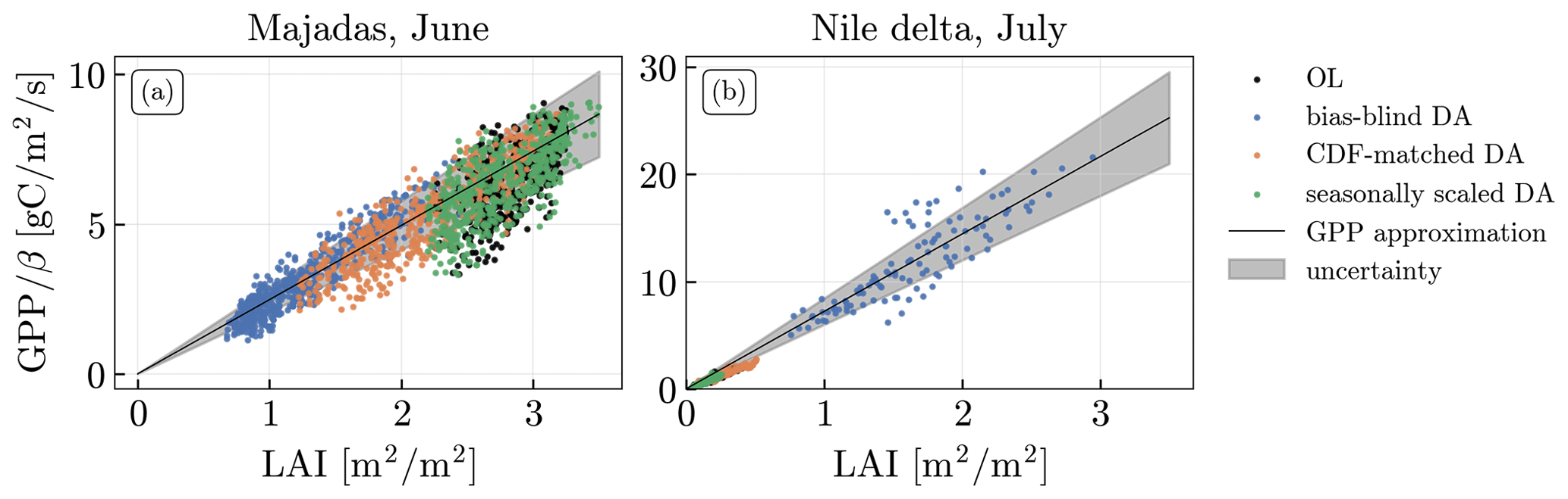
Figure B1 Dependence of soil-moisture-normalised GPP (GPP/β) on LAI for the OL and DA runs, and the linear approximation obtained via a least-squares fit for (a) Majadas in June and (b) the Nile delta in July.

Appendix C: Used ISMN networks

Brocca et al. (2011b)Brocca et al. (2011b)Zreda et al. (2008, 2012)Ikonen et al. (2016, 2018)Al-Yaari et al. (2018)Wigneron et al. (2018)Blöschl et al. (2016)Vreugdenhil et al. (2013)Jensen and Refsgaard (2018)Bircher et al. (2012)Morbidelli et al. (2017)Biddoccu et al. (2016)Raffelli et al. (2017)Alday et al. (2020)Beyrich and Adam (2007)González-Zamora et al. (2019)Calvet et al. (2007, 2016)Albergel et al. (2008)Capello et al. (2019)Darouich et al. (2022)Marczewski et al. (2010)Zacharias et al. (2011)Bogena et al. (2018, 2012)Bogena (2016)Schlenz et al. (2012)Loew et al. (2009)Brocca et al. (2011a, 2008, 2009)Fuchsberger et al. (2021)Kirchengast et al. (2014)Petropoulos and McCalmont (2017)

Table C1 ISMN networks used for evaluation.