A semi-parametric hourly space–time weather generator

Long continuous time series of meteorological variables (i.e. rainfall, temperature and radiation) are required for applications such as derived flood frequency analyses. However, observed time series are generally too short, too sparse in space or incomplete, especially at the sub-daily timestep.

Stochastic weather generators overcome this problem by generating time series of arbitrary length. This study presents a major revision to an existing space–time hourly rainfall model based on a point alternating renewal process, now coupled to a k-NN resampling model for conditioned simulation of non-rainfall climate variables.

The point-based rainfall model is extended into space by the resampling of simulated rainfall events via a simulated annealing optimisation approach. This approach enforces observed spatial dependency as described by three bivariate spatial rainfall criteria. A new non-sequential branched shuffling approach is introduced which allows the modelling of large station networks (N>50) with no significant loss in the spatial dependence structure.

Modelling of non-rainfall climate variables, i.e. temperature, humidity and radiation, is achieved using a non-parametric k-nearest neighbour (k-NN) resampling approach, coupled to the space–time rainfall model via the daily catchment rainfall state. As input, a gridded daily observational dataset (HYRAS) was used. A final deterministic disaggregation step was then performed on all non-rainfall climate variables to achieve an hourly output temporal resolution.

The proposed weather generator was tested on 400 catchments of varying size (50–20 000 km²) across Germany, comprising 699 sub-daily rainfall recording stations. Results indicate no major loss of model performance with increasing catchment size and a generally good reproduction of observed climate and rainfall statistics.

1 Introduction

Stochastic simulation of rainfall has long been an extensive topic of research, with applications including hydrological design, agricultural and water balance models, and for hydrological modelling for derived flood frequency analysis. Through regionalisation techniques, stochastic rainfall models may also be used to generate synthetic time series for ungauged sites.

At the daily timestep, a common approach is to model first the rainfall occurrence (wet or dry) and then the rainfall depth separately. Examples using Markov chains to model rainfall occurrence with probability distributions modelling rainfall depth include Richardson (1981) and Stern and Coe (1984) amongst others, and extended to the multi-site case by Wilks (1998) and Bárdossy and Pegram (2009) via copulas. Alternatively, rainfall occurrence may also be described by an alternating renewal process, that is, sequences of serially independent wet and dry periods (Buishand, 1978), with a random variable describing the event rainfall depth. Non-parametric versions of some of the above-mentioned models which sample from empirical distributions of the modelled variables also exist (Lall et al., 1996). All of the above daily rainfall models are conceptually simple plus given the availability of observed daily rainfall data, easy to apply. However, these models do not necessarily translate well to sub-daily timesteps.

Sub-daily rainfall models are often preferred, especially for flood simulation of smaller catchments. In the urban context, sub-hourly rainfall models may be required to accurately model flash floods, which are ever increasing due to land use changes and the effects of climate change. A common type of sub-daily rainfall model are point process models, which describe the arrival of storm cells in time via a Poisson distribution. Neyman–Scott type models (Rodríguez-Iturbe et al., 1987; Cowpertwait, 1991) and Bartlett–Lewis type models (Onof and Wheater, 1994; Kaczmarska et al., 2014; Onof and Wang, 2020) both model storm cells as a collection of rainfall cells, with varying depths and durations that may overlap. The two types differ in how they describe the timing of storm cells. In Neyman–Scott models, cells are described relative to the beginning of a storm using a Poisson distribution, whereas in the Bartlett–Lewis type, the duration between cell origins is modelled via a random variable. The Newman–Scott type has been extended into space (Cowpertwait et al., 2002; Leonard et al., 2008) by modelling storm spatial extent and cell centre in space. Pegram and Clothier (2001b, a) presented a gridded high-resolution stochastic model in space which mimics and is calibrated from sequences of radar images. Paschalis et al. (2013) expanded on this concept to better describe advective storm cells stochastically in space and time.

Multiplicative cascade models disaggregate rainfall from coarser to finer timesteps. Depending on their principles of mass conservation, they are either described as microcanonical, which strictly conserve mass (Olsson, 1998; Licznar et al., 2011), or canonical, which only on average conserve mass (Molnar and Burlando, 2005). Müller and Haberlandt (2015) further expanded a microcanonical cascade model into space by the resampling of relative diurnal profiles using a simulated annealing optimisation approach.

Alternating renewal type models, already introduced above at the daily timestep, have also been successfully applied at sub-daily timesteps (Tsakiris, 1988; Haberlandt, 1998; Bernardara et al., 2007), including the 5 min timestep for urban applications (Callau Poduje and Haberlandt, 2017). Few attempts have been made to extend these point rainfall models in space, with the exception of Haberlandt et al. (2008). In the study, spatial consistency was applied in a two-step approach. First, time series at single sites were synthesised with no consideration of neighbouring sites. Then, rainfall events were resampled on a site-wise basis via a simulated annealing optimisation procedure conditioned on observed bivariate spatial dependence criteria. A major shortcoming, however, was that the method was only feasible for smaller stations' networks (N≤6).

Extending to non-rainfall climate variables, numerous parametric and non-parametric approaches exist. Richardson (1981) extended a single-site Markov based precipitation model to temperature and solar radiation using a multivariate stochastic process conditioned on the rainfall state (wet or dry). Wilks (1999) improved and extended this type of model into space by using spatially correlated random numbers for synthesis. More recently, Peleg et al. (2017) introduced a gridded high-resolution (2 km grid, 5 min timestep) stochastic weather generator for the modelling of eight meteorological variables, including advective based rainfall. Papalexiou (2018) introduced a general purpose framework to stochastically model arbitrary combinations of hydroclimatic processes at a variety of time scales. Papalexiou (2022) expands on this framework to encompass properties specific to rainfall such as intermittency, marginal distribution and auto-correlation structure for sub-daily time series, however only for single sites.

k-NN resampling is a flexible non-parametric approach which can easily be extended to the multi-site and multi-variate case. Cross correlations between variables are inherently maintained due to simultaneous resampling, and being non-parametric, the approach is suitable for a diverse range of climate variables. Lall and Sharma (1996) used k-NN resampling for generating runoff time series. Daily multi-site rainfall and temperature k-NN models, such as by Buishand and Brandsma (2001), can further be conditioned on regional climate scenarios (Yates et al., 2003) or atmospheric circulation patterns (Beersma and Buishand, 2003). One drawback of k-NN resampling, though, is the inability to simulate values beyond the range of observations. Sharif and Burn (2007) overcame this limitation by introducing a random component to the output. Less common are sub-daily resampling approaches, with most of them in the form of method of fragments disaggregation models which resample diurnal rainfall profiles conditioned on daily rainfall (Mehrotra et al., 2012). The intermittency of rainfall especially at the sub-daily timestep creates challenges for resampling and Markov approaches. Hybrid approaches exist which couple stochastic rainfall models to non-parametric weather generators (Apipattanavis et al., 2007).

The present paper adopts this hybrid approach by coupling a multi-site hourly rainfall model based on an alternating renewal approach (Haberlandt et al., 2008) to a k-NN resampling of non-rainfall variables, coupled via the daily rainfall state (wet, dry, very wet). Innovations to the multi-site rainfall model are introduced and tested at multiple scales, by applying the model to 400 meso-scale catchments of varying size across Germany. The resampling of non-rainfall variables is performed using a daily gridded dataset as observations. As a last step, the daily non-rainfall climate variables are disaggregated to hourly timesteps to match that of the rainfall model. Model validation is achieved by assessing the model's ability to reproduce extreme rainfall at both the site and catchment scale, its ability to reproduce observed spatial rainfall characteristics, the reproduction of observed correlations between rainfall and the non-rainfall variables, and more generally the reproduction of observed point and catchment scale statistics of both rainfall and non-rainfall variables.

2 Methodology

The model chain is divided into four distinct components using two primary observation sources (Fig. 1 for a model chain schematic). The foundation of the weather generator is a stochastic single-site hourly rainfall model based on an alternating renewal process (Sect. 2.1), parametrised using observed hourly station rainfall data. This single-site model is then extended into space by site-wise resampling of rainfall events via a simulated annealing optimisation approach to enforce observed spatial rainfall characteristics of multi-variate non-lagged rainfall time series (Sect. 2.2). Non-rainfall climate variables are modelled using a non-parametric k-NN resampling approach (Sect. 2.3), using a gridded daily climate dataset as observations. The k-NN model is coupled to the space–time rainfall model via the catchment averaged daily rainfall state (dry, wet, very wet). Finally, to achieve the target output temporal resolution, the non-rainfall climate variables are disaggregated from daily to hourly (Sect. 2.4) using the open-source deterministic disaggregation tool MELODIST (Förster et al., 2016).

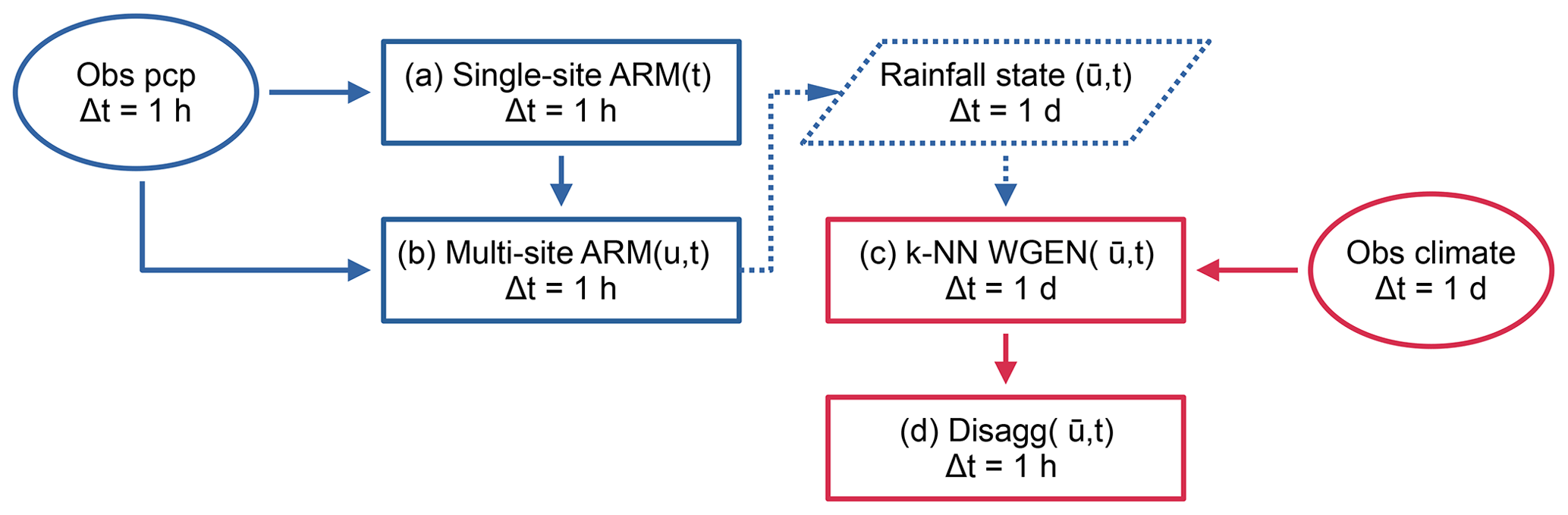
Figure 1 Workflow of the complete model chain. Two primary data sources are utilised, hourly station rainfall observations (left, blue) and a daily gridded climate product (right, red). The foundation and first step of the model chain is the single-site stochastic rainfall model based on an alternating renewal process (a). This model is extended into space u via resampling to enforce observed spatial consistence (b). Non-rainfall climate variables are resampled from catchment averaged observations using a k-NN approach (c), conditioned on the daily catchment averaged rainfall state resulting from (b). Finally, the simulated non-rainfall climate variables are disaggregated from daily to hourly (d) to meet the desired output temporal resolution.

2.1 Single-site stochastic rainfall model

The first step is the generation of synthetic hourly rainfall time series at the site level. For this, an alternating renewal model is used. Rainfall is described as an alternating sequence of independent wet and dry spells. The model shown here is a revision of the model introduced by Haberlandt (1998) and most recently further developed by Callau Poduje and Haberlandt (2017). The model consists of an internal and external structure (Fig. 2). The external structure describes the occurrence of rainfall events. The internal structure describes the temporal distribution of rainfall within a rainfall event (i.e. the event hyetograph).

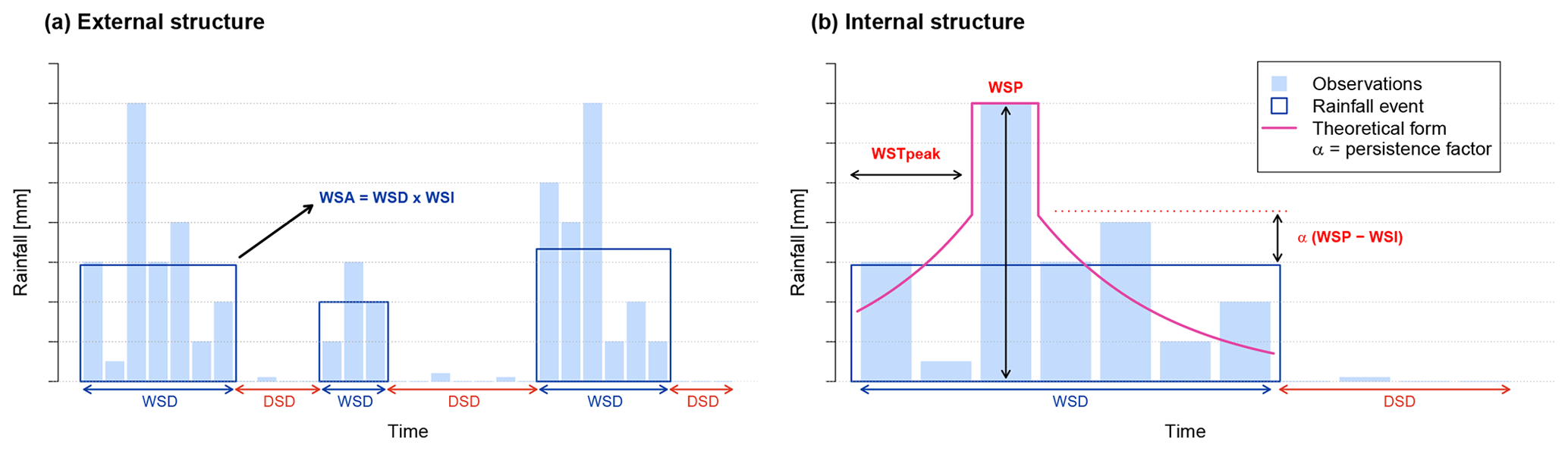
Figure 2 Schematic of the external (a) and internal (b) forms of the alternating renewal single-site rainfall model. Observations are shown as vertical blue bars. Rainfall events are shown by dark blue rectangles. Observations falling outside of rainfall events are below the WSA_min threshold. Events are additionally separated according to the DSD_min threshold. For synthesis, each event is assigned an event hyetograph based on an exponential function (pink curve).

The external structure is the basis of the alternating renewal model and describes the occurrence of rainfall events via the variables wet spell duration (WSD), wet spell amount (WSA) and dry spell duration (DSD). Probability distributions are then fitted to these three event variables using the method of L-moments (Hosking, 1990). Probability distributions for the event variables were chosen over other potential distributions through a combination of visual tests (including L-moment diagrams), goodness-of-fit tests and by evaluating end model performance when using various distributions. Rainfall events are defined here as having a volume above a given threshold, the WSA_min and a minimum separation distance to the next event of DSD_min. In this study, values of WSA_min= 1 mm and DSD_min= 4 h were chosen largely arbitrarily. Auto-correlation of the event variables is not considered, as observed auto-correlations of these variables are generally less than 0.05 even at lag 1.

However, there exists a strong dependence between the event variables WSA and WSD. Copulas are one method routinely used to model such dependencies. A copula describes a multi-dimensional space where the marginal distributions of each variable is transformed to the uniform (i.e. each dimension has the interval [0,1]). Their use in hydrology has been increasing over the years (see Chen and Guo, 2019 for an overview of applications). Copulas can be of any dimension ≥2, but as is most frequently found in the literature and and as used in this study, only copulas of the bivariate case will be discussed from this point onwards.

Considering U and V as the uniformly transformed marginals of the two continuous random variables X and Y, with U=F_X(X) and V=F_Y(Y), a copula C is the bivariate distribution function of U and V:

$$\begin{array}{}\text{(1)}& \begin{array}{rl}{C}_{U,V}(u,v)& =\mathrm{P}(U\le u,V\le v)\\ & =C\left(F_U\right(u),F_V(v\left)\right)\\ & \mathrm{with}C:[\mathrm{0},\mathrm{1}{]}^{\mathrm{2}}\to [\mathrm{0},\mathrm{1}],\mathrm{for}u,v\in [\mathrm{0},\mathrm{1}].\end{array}\end{array}$$

The primary benefit of this transformation is that the marginal distributions of X and Y play no role in describing the dependence between the variables.

Of special importance in this study is the modelling of extreme events with high rainfall intensity. These events by definition tend to have short duration but large rainfall depth. A copula capable of modelling these extreme events should thus be asymmetric (as these events appear in one corner of the copula but not the opposite corner). In the previous version of the model (Callau Poduje and Haberlandt, 2017), the concept of a regional empirical copula was introduced for this purpose. Within the study area, rainfall events were first normalised on a station-wise basis and then appended together to form a study area wide empirical copula. One drawback is that only observed events can be sampled from the copula. Events more extreme than previously observed could never be synthesised. This is particularly problematic as observation lengths are often limited due to relatively few recording stations being available at the sub-daily timestep, especially regarding longer recording periods.

For this study, a Khoudraji–Gumbel copula was chosen to model the WSA–WSD dependence. Selection was again through a combination of visual tests, goodness-of-fit criteria and end model performance. A Khoudraji copula is a device in which two copulas C₁ and C₂ are combined via the equation:

$$\begin{array}{}\text{(2)}& C=C_{\mathrm{1}}(u^{\mathrm{1}-a_{\mathrm{1}}},v^{\mathrm{1}-a_{\mathrm{2}}})C_{\mathrm{2}}(u^{a_{\mathrm{1}}},v^{a_{\mathrm{2}}}),\end{array}$$

with a₁ and a₂ being shape parameters in the range [0,1]. A common use of the Khoudraji copula is to better model asymmetries (i.e. $C(U,V)\ne C(V,U)$). In its use here, an independence copula is selected as C₁ and a single parameter Gumbel (a.k.a. Gumbel–Hougard) copula, which shows greater dependence in the positive tail, as C₂. The second shape parameter a₂ is fixed to 1, meaning that the combined copula is described by two parameters. An independence copula is one where the uniform marginals U and V show no dependence (correlation = 0) and is defined by

$$\begin{array}{}\text{(3)}& C^I(u,v)=uv=C_{\mathrm{1}}.\end{array}$$

The bivariate Gumbel copula is defined by

$$\begin{array}{}\text{(4)}& C_{\mathit{\theta }}^G(u,v)=\exp \left(-{\left[(-\ln u{)}^{\mathit{\theta }}+(-\ln v{)}^{\mathit{\theta }}\right]}^{\mathrm{1}/\mathit{\theta }}\right)=C_{\mathrm{2}},\end{array}$$

and parameterised by $\mathit{\theta }\in [\mathrm{1},\mathrm{\infty })$.

An additional modification from Callau Poduje and Haberlandt (2017) is the use of the Weibull distribution for both the DSD and WSA marginals in place of the Kappa distribution. As Weibull is a three-parameter distribution versus Kappa's four, better model parsimony has been achieved without any significant loss of performance. This is also of benefit in any regionalisation setting. The cumulative distribution function for the Weibull distribution is defined by

$$\begin{array}{}\text{(5)}& F\left(x\right)=\mathrm{1}-\exp \left[-{\left({\displaystyle \frac{x+\mathit{\zeta }}{\mathit{\beta }}}\right)}^{\mathit{\delta }}\right],\end{array}$$

with x>0, ζ≥min(x) a location parameter, β>0 a scale parameter and δ>0 a shape parameter.

The WSD is modelled using the three-parameter log normal distribution defined by

$$\begin{array}{}\text{(6)}& F\left(x\right)=\mathrm{\Phi }\left[{\displaystyle \frac{\log \left(x-\mathit{\zeta }\right)-{\mathit{\mu }}_{\log }}{{\mathit{\sigma }}_{\log }}}\right],\end{array}$$

with Φ being the cumulative distribution function of the standard normal distribution, ζ the lower bound (real space) of x and μ_log and σ_log being the mean (location parameter) and standard deviation (scale parameter), respectively, of x in the natural logarithmic space.

The internal model structure describes the temporal distribution of rainfall within a rainfall event, in other words the event hyetograph (Fig. 2b). The following exponential function is used to disaggregate the event rainfall intensity WSI over each timestep within an event:

$$\begin{array}{}\text{(7)}& \begin{array}{rl}& P\left(t\right)=\left\{\begin{array}{ll}\mathrm{WSP}\cdot {\mathrm{e}}^{\left[c\mathit{\lambda }(t-\mathrm{WSPT})\right]\mathit{\alpha }}& \mathrm{if}t\ne \mathrm{WSPT}\\ \mathrm{WSP}& \mathrm{if}t=\mathrm{WSPT}\end{array}\right.\\ & \mathrm{with}c=\left\{\begin{array}{ll}+\mathrm{1}& \mathrm{if}t<\mathrm{WSPT}\\ -\mathrm{1}& \mathrm{if}t>\mathrm{WSPT}\end{array}\right.,\end{array}\end{array}$$

with P being the rainfall intensity for timestep t, WSP the wet spell peak intensity and WSPT the timestep of the wet spell peak. λ is solved numerically for each event separately, and the WSPT is sampled from a uniform distribution. α is used to adjust the shape of the exponential curve relative to the WSP (Fig. 2) and as per Callau Poduje and Haberlandt (2017) is set to $\mathrm{1}/\mathrm{3}$.

Differently to what is presented in Callau Poduje and Haberlandt (2017), the WSP is now modelled by fitting a Weibull distribution (Eq. 5) to the ratio WSP : WSA. Events with a length equal to the timestep (1 hour) are first excluded. This restricts the range of possible values to between (0,1). A Khoudraji–Gaussian copula then models the dependence of the ratio WSP : WSA to WSD. Here, too, use of an asymmetric copula via Khoudraji's device (again with a fixed second shape parameter = 1 and an independence copula as C₁ as per Eq. 2) showed the best results. The bivariate normal copula is defined by Eq. (8). The previous model relied on a symmetrical Gaussian copula to describe the dependence between WSP and the event wet spell intensity ($\mathrm{WSI}=\mathrm{WSA}/\mathrm{WSD}$). This approach was problematic during synthesis, as wet spell peaks could be sampled producing a wet spell peak greater than the event WSA. The new method avoids this issue. The normal copula is defined as

$$\begin{array}{}\text{(8)}& C_{{\mathit{\varphi }}^R}^G(u,v)={\mathit{\varphi }}_R\left({\mathit{\varphi }}^{-\mathrm{1}}\left(u\right),{\mathit{\varphi }}^{-\mathrm{1}}\left(v\right)\right)=C_{\mathrm{2}},\end{array}$$

with ϕ_R being the joint bivariate Gaussian distribution function with correlation matrix R for u and v, and ϕ⁻¹ being the inverse normal cumulative distribution function.

The rainfall event definition (requiring WSA ≥WSA_min, DSD ≥DSD_min) leads to a systematic underestimation of total rainfall. As a final step, small events (rainfall events below the WSA_min threshold) are added to the time series. The method simply resamples (with replacement) small events from observations until the observed proportion of small to large rainfall events is met. Small event depth, duration and distance to the next adjacent large event are sampled simultaneously and placed randomly in dry spells of adequate length.

2.2 Space–time rainfall synthesis via resampling

Following generation of single-site rainfall time series, rainfall events are then resampled to reproduce observed spatial rainfall dependence across a catchment. Specifically, the method aims to preserve the rainfall occurrence, correlation, and continuity of concurrent timesteps between station pairs within the network. As only concurrent (i.e. non-lagged) timesteps are considered, lagged spatial rainfall effects such as advection are neither considered nor reproduced. The resampling procedure is an extension of the simulated annealing optimisation approach described by Haberlandt et al. (2008). By reshuffling rainfall events (as opposed to hourly timesteps), the independence of rainfall events at single sites, as is a pre-condition of the alternating renewal model, is maintained.

Simulated annealing is a discrete optimisation procedure which is well suited to finding global minima or maxima (Bertsimas and Tsitsiklis, 1993). The method as presented here minimises an objective function describing spatial rainfall dependence by swapping rainfall events at sites at random. All reductions in the objective function are accepted, however swaps which result in an increase can also be accepted with a probability relative to the current annealing temperature. The annealing temperature decreases as the algorithm proceeds, making it less and less likely that bad swaps will be accepted. By sometimes accepting a worse objective function result, the algorithm avoids becoming stuck in local minima and aids in finding the global minimum.

As we are attempting to recreate observed spatial rainfall dependence, the objective function incorporates three bivariate rainfall dependence criteria. The first describes the probability of simultaneous rainfall occurrence at station pair k and l:

$$\begin{array}{}\text{(9)}& P_{k,l}(z_k>\mathrm{0}|z_l>\mathrm{0})={\displaystyle \frac{n_{\mathrm{11}}}{n}},\end{array}$$

where n₁₁ is the number of timesteps with simultaneous rainfall occurrence at stations k and l, and n is the total number of (non-missing) timesteps.

The second criterion describes the Pearson correlation of simultaneous rainfall at both k and l:

$$\begin{array}{}\text{(10)}& {\mathit{\rho }}_{k,l}(z_k>\mathrm{0}|z_l>\mathrm{0})={\displaystyle \frac{\mathrm{cov}(z_k,z_l)}{\sqrt{\mathrm{var}\left(z_k\right)\times \mathrm{var}\left(z_l\right)}}},\end{array}$$

where z_k and z_l are timesteps with rainfall at k and l.

Lastly, the third criterion is a continuity measure proposed by Wilks (1998) and is the ratio of the expected rainfall at station k for timesteps with and without simultaneous rainfall at station l:

$$\begin{array}{}\text{(11)}& C_{k,l}={\displaystyle \frac{E\left(z_k\right|z_k>\mathrm{0},z_l=\mathrm{0})}{E\left(z_k\right|z_k>\mathrm{0},z_l>\mathrm{0})}}.\end{array}$$

A continuity close to one describes independent stations, whereas values approaching zero describe increased dependence.

In the paper by Haberlandt et al. (2008), these three spatial rainfall criteria were combined into one objective function as follows:

$$\begin{array}{}\text{(12)}& \begin{array}{rl}{O}_{k,l}=& w_P\times (P_{kl}-P_{kl}^{*}{)}^{\mathrm{2}}+w_{\mathit{\rho }}\times ({\mathit{\rho }}_{kl}-{\mathit{\rho }}_{kl}^{*}{)}^{\mathrm{2}}\\ & +w_C\times (C_{kl}-C_{kl}^{*}{)}^{\mathrm{2}},\end{array}\end{array}$$

for stations k and l with w_P, w_ρ, and w_C being weights above zero to account for the effect of differing scales between the three criteria, and ^* denoting target values. Target values can be assigned either by fitting regression curves to observed values as a function of station separation distance, or by using observed values directly. In this study the first approach is taken in order to demonstrate the method's applicability in regionalisation settings. However, as direction between station pairs is not considered, any anisotropic properties of the three criteria will not be reproduced.

Experimentation showed that splitting the three-part objective function into two separate objective functions could lead to a faster and more optimal convergence. Of the three criteria, the occurrence criterion is by far the hardest to converge. In addition, the Pearson correlation criterion shows high sensitivity and tends to dominate over the other two criteria. Selecting appropriate weights to counteract discordance between the three criteria also proved to be problematic. Therefore, the optimisation procedure was split into a two-step process, where first the occurrence criterion (Eq. 9) is converged (step I), followed together by the correlation (Eq. 10) and continuity (Eq. 11) criteria (step II). However, for this to be possible in the second step, only events of equal length are swapped, in order to maintain the rainfall occurrence which was already optimised in step I. At low station counts the benefit of such an approach is negligible, however with increasing station count (N>20), such a method can halve the computational time required and shows increased overall performance.

In the study by Haberlandt et al. (2008), stations were shuffled in sequence. That is, the first station was left unchanged, then the second station was shuffled against the first, then the third against both the first and second and so forth. It was shown that such an approach is only effective up to station counts of around 5, as with each additional station, the resampling becomes less and less flexible due to fewer and fewer degrees of freedom.

To overcome this, a new shuffling procedure is introduced in this study, best described as a non-sequential approach. Non-sequential here describes the fact that stations are no longer shuffled sequentially across the entire station network, but rather simultaneously. So for a given annealing temperature, swaps are performed among all stations at random allowing for a more flexible and rapid convergence.

The simulated annealing shuffling algorithm is thus as follows. Let U be the set of all stations to be shuffled, k be the station currently having two events swapped and R be the set of reference stations for which the objective function is calculated for k, with $R=U,k\notin R$.

1. The algorithm begins at step I, considering only the rainfall occurrence (Eq. 9).

2. An initial annealing temperature T_a is chosen. Experience shows that an annealing temperature resulting in an initial swap count of ≈ 80 % is optimal (Bárdossy et al., 2002).

3. A station k is chosen at random from all eligible stations within the set U.

4. The initial objective function O_k,prev is calculated for station k using Eq. (13) if step I or Eq. (14) if step II, with $l=\mathrm{1},\mathrm{\dots },M$ being the set of reference stations R.

   $$\begin{array}{}\text{(13)}& {\displaystyle }{O}_k=\sqrt{{\displaystyle \frac{{\sum }_{l=\mathrm{1}}^M(P_{kl}-P_{kl}^{*}{)}^{\mathrm{2}}}{M}}},\text{(14)}& {\displaystyle }\begin{array}{rl}{O}_k& =w_{\mathit{\rho }}\sqrt{{\displaystyle \frac{{\sum }_{l=\mathrm{1}}^M({\mathit{\rho }}_{kl}-{\mathit{\rho }}_{kl}^{*}{)}^{\mathrm{2}}}{M}}}\\ & +w_C\sqrt{{\displaystyle \frac{{\sum }_{l=\mathrm{1}}^M(C_{kl}-C_{kl}^{*}{)}^{\mathrm{2}}}{M}}}.\end{array}\end{array}$$

5. Two rainfall events from station k are chosen at random to be swapped with the following pre-condition.

   • For step I, the events must be within an allowed temporal distance (here, six events). This allows a quicker and smoother convergence as the sensitivity of the objective function from swaps is greatly reduced.

   • For step II, only events of equal length my be swapped, in order to avoid invalidating the occurrence objective criterion previously converged in step I.

6. An updated objective function O_k,new is calculated to reflect the swap.

7. If $O_{k,\mathrm{new}}<O_{k,\mathrm{prev}}$, then the swap is accepted.

8. If O_k,new ≥ O_k,prev, the swap is accepted with the probability π:

   $$\begin{array}{}\text{(15)}& \mathit{\pi }=\exp \left({\displaystyle \frac{O_{k,\mathrm{prev}}-O_{k,\mathrm{new}}}{T_{\mathrm{a}}}}\right).\end{array}$$

   where T_a is the current annealing temperature.

9. Repeat sub-steps 3–8 N times.

10. The annealing temperature T_a is reduced:

    $$\begin{array}{}\text{(16)}& T_{\mathrm{a}}=T_{\mathrm{a}-\mathrm{1}}\times \mathrm{d}T,\end{array}$$

    with dT being the temperature reduction factor in the range $\mathrm{0}<\mathrm{d}T<\mathrm{1}$. Generally, a slow reduction in temperature is best (i.e. dT≈0.98). After reducing the annealing temperature, proceed once more from sub-step 3.

11. The current step is stopped when the mean improvement of the objective function across all stations between temperature reductions is below a certain threshold, or if the mean objective function across all stations is below a certain target value.

12. If step I, the algorithm proceeds again from sub-step 2, with step II now considering together the correlation (Eq. 10) and continuity (Eq. 11), otherwise the optimisation is complete.

Lastly, it was shown that the shuffling process can be further optimised if large station networks are branched into groups, similarly to the approach by Müller and Haberlandt (2015). This is not absolutely necessary for successful convergence, but was shown to both increase performance and decrease computational effort, especially for very large networks (N≥20). A group size of 4 was used in this study, and groups are formed in a way that maximises the minimum distance between group midpoints. At each annealing temperature, shuffling (sub-steps 3–8) occurs on a group-wise basis in random order. For any group, U is restricted to group members, but R is expanded to include stations external to the group in order to transfer spatial dependence information between groups so that a consistent result is obtained across the entire study area. These additional stations, selected by closest distance, are included in R for the calculation of the objective function but are not included in the set U from which station k is selected for swapping. In this study, up to 16 additional stations were added to R in step I and up to 24 for step II.

For very large networks (N≥20), a further modification is to select from each group a single station to act as a parent station, with all other stations classed as child stations. The shuffling procedure is then first performed for parent stations alone (i.e. both R and U are restricted to parent stations), after which they are fixed (removed from U but remaining in R) for the further shuffling of the child stations. This allows the wider scale transfer of spatial dependence information across the network. Again, this modification is not absolutely necessary but may lead to both a better and faster overall convergence. This is the version ultimately used for this study for all catchments comprising eight or more stations.

2.3 k-NN non-parametric weather generator

Non-rainfall climate variables are modelled using a non-parametric k-NN approach. Non-parametric approaches have the benefit of not needing to assume any underlying distributions of the modelled variables. Traditional k-NN weather generators resample target variables simultaneously for day t with replacement from observations, conditioned on the previous day t−1. As the name implies, k-NN selects a possible k candidate observations for resampling, selected by a distance metric between the feature vectors for day t−1 of the simulation and the candidate observations. The day following the selected observation is then inserted directly as day t of the simulation. As target variables are resampled simultaneously, cross correlations between target variables are inherently maintained. The conditioning on the previous day of the simulation aids in preserving the auto-correlation of the target variables.

In this study, the k-NN resampling is further conditioned on the catchment averaged rainfall state S, which is the mechanism used to couple the space–time rainfall model to the k-NN model. Conditioning on the rainfall state aims to preserve correlations between the target variables and the already simulated catchment rainfall and is based on the method by Apipattanavis et al. (2007).

As the observed climate dataset used in this study is a gridded daily dataset, resampling occurs at the daily timestep. The catchment averaged rainfall state S describes the daily areal rainfall of a catchment as either dry, wet, or very wet. The corresponding rainfall depths which describe these states are taken as the 50th and 95th percentiles of daily rainfall (P_dry<0.5; $\mathrm{0.5}\le P_{\mathrm{wet}}<\mathrm{0.95}$; $P_{\mathrm{v}.\mathrm{wet}}\ge \mathrm{0.95}$). Rainfall acts here purely as a conditioning variable for the k-NN resampling of non-rainfall climate variables, and is not itself resampled.

For each day of the simulation, candidate days from observations are chosen using a moving window ±w around the current simulation day t. For example, if t is 15 June and w=7 d, only observed days between 8 and 22 June (from any year) may be chosen. This enables the reproduction of seasonal climate characteristics.

Potential neighbours are then further reduced by conditioning by rainfall state S for both days t and t−1 of the simulation. For example, if simulated day t is wet and simulated day t−1 very wet, only observed days which are very wet followed by a wet day (and within the observation window ±w) may be chosen. If no days from observations match this criteria, this conditioning is relaxed to apply to day t only.

Feature vectors D are created for each day of observations, with D consisting of the normalised catchment averaged variables x^′. Each climate variable x is first normalised by subtracting the mean and dividing by the standard deviation:

$$\begin{array}{}\text{(17)}& x^{\prime }={\displaystyle \frac{x-\stackrel{\mathrm{‾}}{x}}{\sqrt{\mathrm{var}\left(x\right)}}}.\end{array}$$

The k-NN procedure proceeds as follows:

• a.

  For the first day of the simulation t=1, an observed day within the selection window ±w is selected at random conditioned only on the rainfall state S_t.

• b.

  The simulation day t is advanced by 1.

• c.

  Observed days within the selection window ±w are selected to form candidate days U.

• d.

  U is reduced by conditioning on the rainfall state S_t and S_t−1.

• e.

  A distance metric, the weighted Euclidean distance $\mathit{\delta }({\mathit{D}}_{t-\mathrm{1}},{\mathit{D}}_u)$, is calculated for each day u in U and simulation day t−1:

  $$\begin{array}{}\text{(18)}& \mathit{\delta }({\mathit{D}}_{t-\mathrm{1}},{\mathit{D}}_u)={\left[{\displaystyle }\sum _{j=\mathrm{1}}^N{w}_j(x_{t-\mathrm{1},j}^{\prime }-x_{u,j}^{\prime }{)}^{\mathrm{2}}\right]}^{\mathrm{1}/\mathrm{2}},\end{array}$$

  with w_j being the weight for climate variable $x_j^{\prime }$, N the total number of climate variables, $x_{t-\mathrm{1},j}^{\prime }$ and $x_{u,j}^{\prime }$ being the normalised climate variable for day t−1 and candidate day u. For this study, variable weights were assigned manually by trial and error. A higher weight for one variable over another will generally improve the performance of that variable regarding its correlation to rainfall.

• f.

  Candidate days are then ordered from nearest to farthest and given ranks j.

• g.

  U is then further reduced to k neighbours based on lowest rank (closest distance). The selection of k is user definable but is often taken as $k=\sqrt{N}$ where N is the sample size, as proposed by Lall and Sharma (1996). As the window size ±w restricts possible neighbours, $k=\sqrt{Y\times (\mathrm{2}w+\mathrm{1})}$, with Y equal to the length of observations in years.

• h.

  A single day is then selected from U using a discrete probability distribution. Lall and Sharma (1996) recommended a kernel which gives increased weight to nearer neighbours:

  $$\begin{array}{}\text{(19)}& p_j={\displaystyle \frac{\mathrm{1}/j}{\sum _{i=\mathrm{1}}^k\mathrm{1}/i}},\mathrm{for}j=\mathrm{1},\mathrm{\dots },k.\end{array}$$
• i.

  Day t of the simulation is then taken as day u+1.

• j.

  The algorithm begins again from step b until all days have been simulated.

Figure 3 Box plot of catchment area (N=400).

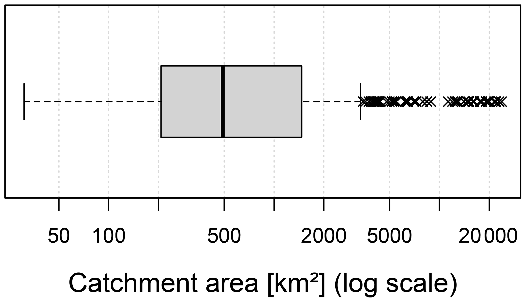
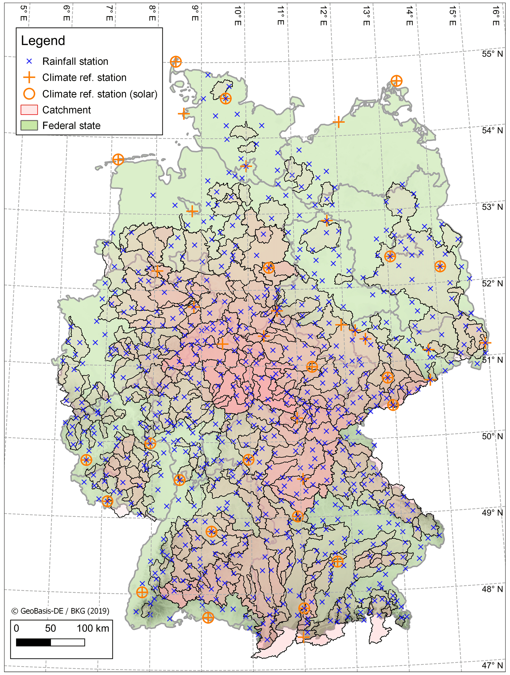
Figure 4 Study area showing location of DWD rainfall stations (N=699), DWD climate stations (N=39) and catchments (N=400). Catchments may be overlapping.

The choice of which combination of climate variables to resample depends largely on the intended end-use of the simulation and the availability of observations. As the feature vector D contains normalised climate values, variables of any magnitude and distribution may be used. Heavily skewed variables may undergo an optional log transformation. For this study, relative humidity, temperature (daily mean, minimum and maximum) and global radiation were chosen, as the intended end-use is derived flood frequency analysis using the hydrological model HBV (Lindström et al., 1997). HBV requires rainfall, temperature and potential evaporation as input, which can all be directly used or derived from these chosen variables. Furthermore, due to ease of use and availability, a gridded observational climate dataset was used for this study. However, the k-NN resampling approach presented is not limited to gridded datasets and may be applied to networks of point observations, with the feature vector D representing mean values across the station network.

2.4 Disaggregation from daily to hourly

A final step is required to disaggregate the resampled daily catchment-averaged non-rainfall climate variables from daily to hourly. This is achieved using the open-source disaggregation tool MELODIST (Förster et al., 2016) which applies deterministic disaggregation functions to a variety of meteorological variables. This tool offers the user several forms of disaggregation, depending on the level of complexity sought and the availability of observations for parameter calibration. For this study, the forms chosen do not rely on hourly observations and instead rely on geographic position (catchment midpoint) only.

Temperature is first disaggregated to hourly values T_d,h for day d and hour h using the cosine function (Debele et al., 2007):

$$\begin{array}{}\text{(20)}& \begin{array}{rl}{T}_{\mathrm{d},\mathrm{h}}& =T_{\min ,\mathrm{d}}+(T_{\min ,\mathrm{d}}+T_{\max ,\mathrm{d}})/\mathrm{2}\\ & \times \left(\mathrm{1}+\cos \left(\mathit{\pi }\right(h+a)/\mathrm{12})\right),\end{array}\end{array}$$

with T_min,d and T_max,d being the minimum and maximum temperatures for day d. The parameter a describes the time difference between solar noon and the time of maximum daily temperature. For this study, a is simplified to two hours across the entire year.

Humidity relies on already disaggregated hourly temperature data. Relative humidity for hour h for day d is calculated by

$$\begin{array}{}\text{(21)}& H_{\mathrm{d},\mathrm{h}}=\mathrm{100}\cdot {\displaystyle \frac{e_{\mathrm{s}}\left(T_{\mathrm{dew},\mathrm{d}}\right)}{e_{\mathrm{s}}\left(T_{\mathrm{d},\mathrm{h}}\right)}}\left[\mathit{\%}\right],\end{array}$$

with e_s being the saturation vapour pressure of a given temperature T [^∘C], given by the Magnus formula (Alduchov and Eskridge, 1997)

$$\begin{array}{}\text{(22)}& e_{\mathrm{s}}\left(T\right)=\left\{\begin{array}{ll}\mathrm{6.1078}\exp \left(\frac{\mathrm{17.08085}T}{\mathrm{234.175}+T}\right)& T\ge \mathrm{0}{}^{\circ }\mathrm{C}\\ \mathrm{6.1071}\exp \left(\frac{\mathrm{22.4429}T}{\mathrm{272.44}+T}\right)& T<\mathrm{0}{}^{\circ }\mathrm{C}\end{array}\right..\end{array}$$

The dew point temperature is simplified and taken as the daily minimum temperature ($T_{\mathrm{dew},\mathrm{d}}=T_{\min ,\mathrm{d}}$) and is constant throughout the day (no diurnal profile). Finally, global shortwave radiation is disaggregated from daily values using a simplified formula which assumes a flat surface (Liston and Elder, 2006):

$$\begin{array}{}\text{(23)}& R_{\mathrm{0}}=\mathrm{1370}{\mathrm{Wm}}^{-\mathrm{2}}\cdot \cos Z_{\mathrm{d},\mathrm{h},\mathit{\varphi }}\cdot ({\mathit{\psi }}_{\mathrm{dir}}+{\mathit{\psi }}_{\mathrm{dif}})\left[{\mathrm{Wm}}^{-\mathrm{2}}\right],\end{array}$$

with ψ_dir and ψ_dif being the direct and diffuse radiation scaling values, $Z_{\mathrm{d},\mathrm{h},\mathit{\varphi }}$ being the local solar zenith angle for day d, hour h and latitude ϕ, which for this study is taken as the mid-point of each catchment. Further details of the radiation scaling values can be found in Liston and Elder (2006).

3 Study area and data

For this study, 400 meso-scale catchments in Germany were selected. These catchments range in size from 30 km² to over 20 000 km². Figure 3 shows a box plot of catchment by area.

As observed rainfall, 699 point sub-daily recording stations at the hourly timestep were sourced from the German Weather Service (DWD) (DWD Climate Data Center, 2021a). A common time period of January 2006–December 2020 was chosen to maximise station availability over the period across all stations. Figure 4 displays the location of both catchments and rain gauges.

Stations are assigned to catchments, and the space–time weather generator is applied on a catchment basis. The largest catchment contains 87 stations, with 109 catchments containing at least 10 stations, and 27 catchments containing at least 30 stations.

The HYRAS (Razafimaharo et al., 2020; DWD Climate Data Center, 2021b) gridded (5 km × 5 km) daily observational climate dataset was chosen for use for the non-rainfall climate variables. Climate variables include the mean, maximum and minimum daily temperature, relative humidity, and global radiation. Coverage of this dataset is German wide, extending into neighbouring countries except Czech Republic. This results in a few catchments with boundaries extending into Czech Republic not having 100 % pixel coverage. For use in the k-NN weather generator, catchment averages were calculated for each catchment and climate variable. The time period 1976–2015 (40 years) was chosen to increase the total number of days available for resampling.

To validate the weather generator results, 40 sub-daily reference climate stations (DWD Climate Data Center, 2021a) were chosen across Germany (Fig. 4). Of these, 20 also include data for global radiation.

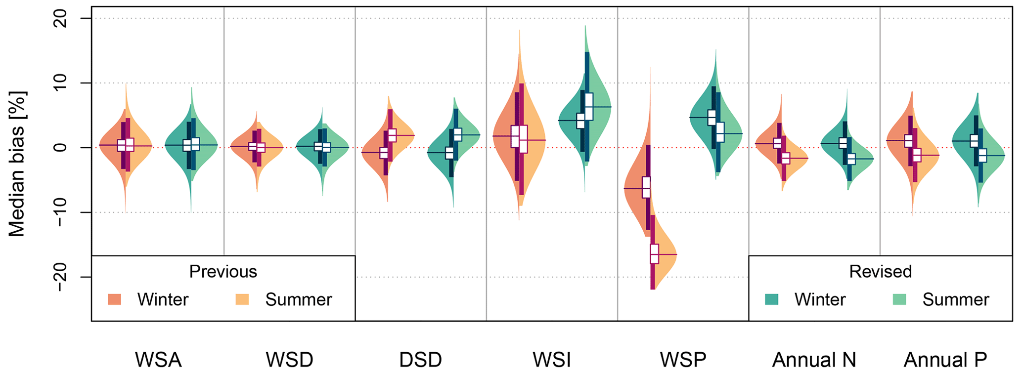
Figure 5 Violin plots of the median bias from 100 × 15 year simulations for 699 rainfall stations. The left side of the violin plot shows results for winter, the right side for summer. Annual N refers to the mean number of annual rainfall events and Annual P the mean annual rainfall sum (before the addition of small events).

The climate of the study area is generally temperate, tending towards continental in the east and southeast and oceanic in the north. Convective precipitation is typical in the summer months, this being a reason why the parametric models presented here were applied to summer and winter separately. Annual rainfall sums range from around 500 mm to over 2000 mm in southern elevated regions. Rainfall is common year round, being the highest in summer and the lowest in spring. Elevations are typically below 1000 m above sea level except in the southern Alpine region. Large temperature gradients are not present, with the warmest area being the Rhine valley along the border with France.

4 Model set-up and validation

To adequately test the performance of the complete model chain, 100 realisations of 15 years simulation length were generated; 15 years was chosen to match the observation length of the sub-daily rainfall stations. The model is conditioned on summer (April–September) and winter (October–March) seasons separately. A conditioning on calendar month would of course have been possible, but due to the limited observation length, a coarser conditioning by season ensures a sufficient number of observations leading to a more robust parametrisation.

Target values as used in the objective function of the simulated annealing resampling procedure were calculated as follows. For each catchment, the closest 100 (at least) to 150 (at most) stations from the centroid of the catchment were selected (this may also include stations located outside of the catchment boundary). For each station pair, the three bivariate spatial rainfall criteria were calculated from observations. Regression curves (not shown here) were then fitted to the observed data with station separation distance as the independent variable. The target values for simulations were then taken from these curves with added noise equal to the residual variance.

For the evaluation criteria, relative bias is calculated as follows:

$$\begin{array}{}\text{(24)}& \mathrm{Bias}=\mathrm{100}\times {\displaystyle \frac{X_i^{*}-X_i}{X_i}}\left[\mathit{\%}\right].\end{array}$$

where X_i is the observed value of the variable in question for station i and $X_i^{*}$ the simulated value. A positive bias indicates overestimation, a negative bias underestimation.

The performance of the weather generator is evaluated as described in the sub-sections below.

4.1 Point rainfall model

The point rainfall model (Sect. 2.1) was applied in two modes for all 699 rainfall stations. The first mode is the model as described by Callau Poduje and Haberlandt (2017) and will be referred to as the “previous” model. The second mode incorporates the changes as introduced in this paper, and is referred to as the “revised” model. The two modes allow us to directly assess whether changes to the rainfall model have, indeed, increased its performance. Note that as the previous model has a target output timestep of 5 min, it may perform less well at an hourly timestep.

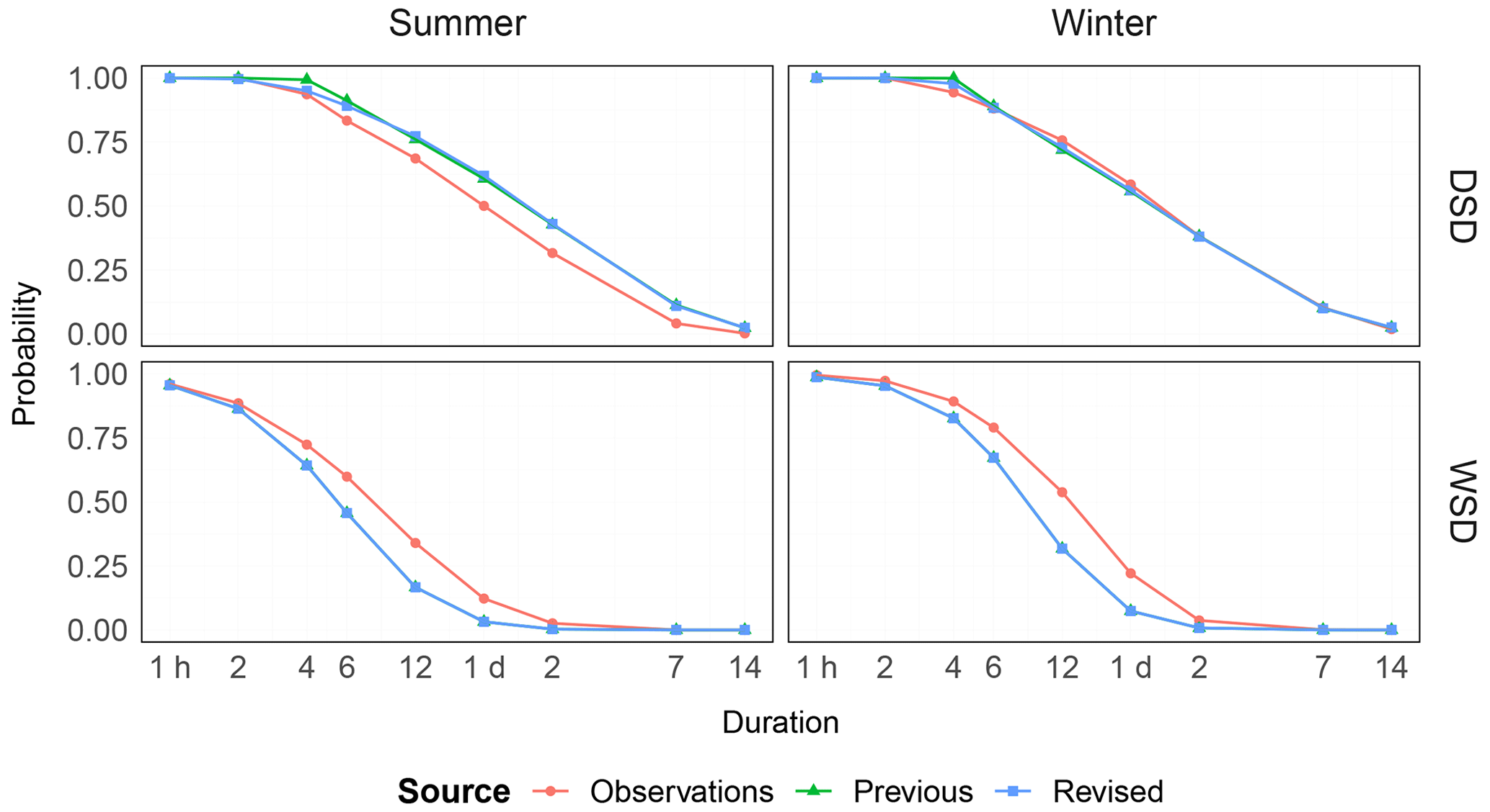
Figure 6 Exceedance probabilities of the event variables WSD and DSD for varying durations, split by season, for both the previous and revised models and compared to the empirical value from observations. The mean over all stations is shown.

The performance is assessed via the following:

• Relative bias of annual precipitation sum and number of events. The median bias for each station over 100 realisations is taken.

• Relative bias of the event variables WSA, WSD, DSD, WSI and WSP. Note that WSI is indirectly modelled but acts as a good indicator of the performance of the bivariate copula C(WSA,WSD). The median bias for each station over 100 realisations is taken.

• Exceedance probabilities for given durations for both WSD and DSD. The mean result over all stations is taken and shown for winter and summer.

• Extremes are assessed via the relative bias in fitted intensity duration frequency (IDF) curves. IDF curves were fitted to observed and simulated (100 × 15 years) annual maxima series using the robust method according to Koutsoyiannis et al. (1998) for the storm durations 1, 3, 6, 12, 24 and 48 h. For each storm duration, the rainfall depth for a return period of 20 years was calculated. The median bias across realisations is then calculated for each station and presented in box plots for each storm duration.

• The wet/dry intermittence of daily rainfall, first by considering wet day frequencies and wet–wet/dry–wet transition probabilities (and by implication their complements, wet–dry/dry–dry transition probabilities). These are presented in observed versus simulated plots. A threshold of ≥ 0.1 mm was used to classify wet days.

4.2 Space–time rainfall model

After the generation of point rainfall, the model was extended into space on a catchment-wise basis by applying the simulated annealing resampling approach described in Sect. 2.2. Due to computational constraints, the previous model is not considered here. The performance in space is assessed via the following:

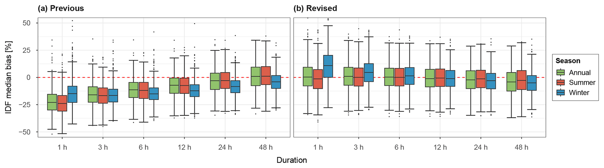
Figure 7 Box plots of median IDF bias over 100 realisations for all stations across the study area (N=699) for various storm durations, split by season, for both the previous (a) and revised models (b). A return period of 20 years has been used.

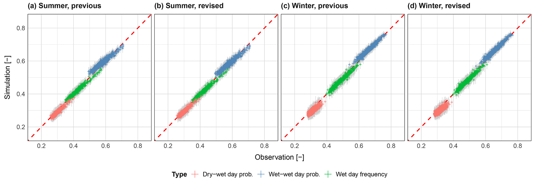
Figure 8 Daily wet day statistics for all stations across the study area (N=699), for both the previous and revised models, split across seasons. Grey lines show the range of results across 100 realisations. The dry–dry and wet–dry transition probabilities, and the dry day frequency, can be inferred from the plots using the complement.

• Spatial dependence of hourly rainfall via the three bivariate criteria (occurrence, correlation and continuity) presented as a 2D density plot. To produce the empirical densities, for each station pair the median result across all realisations was taken.

• Like for the point rainfall model (see above), the bias in fitted areal IDF curves, again incorporating the storm durations 1, 3, 6, 12, 24 and 48 h with a return period of 20 years, was calculated for each catchment and presented as box plots. Catchment rainfall was calculated via the Thiessen polygon method.

4.3 Non-rainfall climate variables

The non-rainfall climate variables are first assessed at the daily timestep to isolate errors stemming from the k-NN resampling. The performance for catchment averaged values is assessed via the following:

• Summary statistics of modelled climate variables comparing mean monthly observed vs. simulated values.

• For each of the modelled climate variables, the daily auto-correlations up to lag 7 is shown plotted on observed vs. simulated plots.

• Daily correlation between rainfall vs. non-rainfall climate variables plotted on observed vs. simulated plots, shown by month.

Also of interest is how well the k-NN resampling approach performs considering point observations. For this, 39 reference weather stations were taken from the German Weather Service observation network and compared to first, (a) the grid cell values taken directly from the HYRAS observational dataset in order to first assess bias resulting from the gridded dataset, and secondly, (b) the k-NN resampled values by taking the median result over 37 × 40 year simulations. Monthly mean values are shown on observed vs. simulated plots.

Finally, the bias due to disaggregation from daily to hourly is assessed by comparing hourly means of each climate variable averaged across each reference station. As the intended use of the weather generator is for applications such as derived flood frequency analyses, the performance of the hourly non-rainfall variables is of lower priority.

5 Results and discussion

5.1 Point rainfall model

Figure 5 shows violin plots of the median bias of event variables, the number of annual events, and the total annual precipitation sum. For the event variables WSD, DSD and WSI, the previous and revised models perform almost identically. This demonstrates that the change from the four-parameter kappa distribution to the three-parameter Weibull distribution for the variables WSA and DSD has no negative consequence on model performance. Of the directly modelled event variables, DSD shows the worst performance, and more so for summer, indicating that an alternative distribution function may be more appropriate.

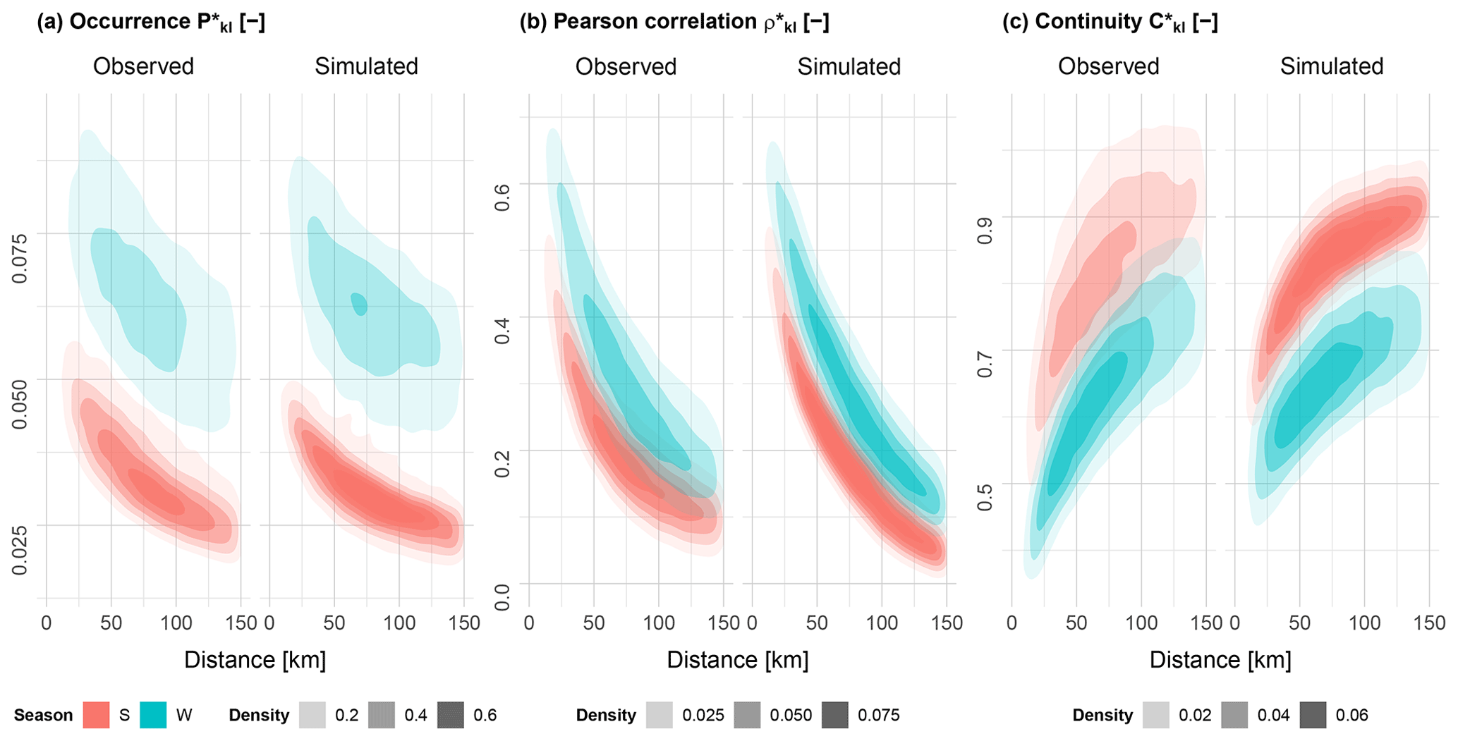
Figure 9 2D density plots of the occurrence (a), Pearson's correlation (b) and continuity (c) bivariate spatial dependence criteria, grouped by season, for all station pairs across all catchments (N=19 773), by station distance. For simulated results, the median value from 100 realisations was taken.

The revised model shows decreased performance regarding wet spell intensities. Wet spell intensities are indirectly modelled via the WSA : WSD copula. The previous model implements a so-called regional empirical copula, which resamples from observations. As the median bias shown in the violin plot directly compares simulated versus observed values, it may be that this statistic favours the previous model due to this resampling. On the other hand, the revised model shows a substantially better modelling of the wet spell peak, which validates the new wet spell peak modelling approach. Except for WSP and WSI, the bias for all other variables lies within ±10 % range.

Finally, in terms of annual number of events and rainfall sum, both models perform similarly well, with summer showing a greater underestimation and winter a more moderate overestimation. This is likely due to a mean overestimation of DSD in summer as was discussed above. Here, bias also lies within a ±10 % range.

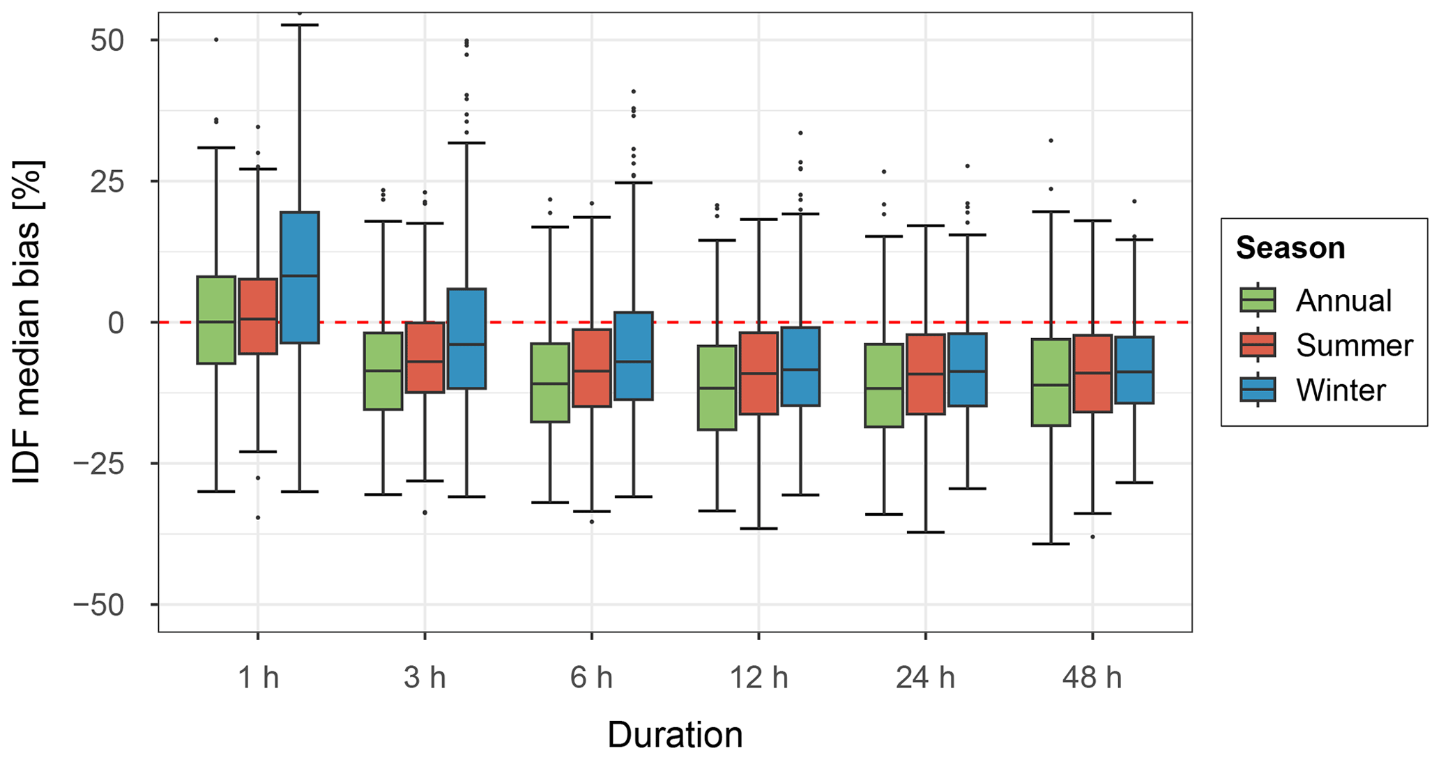
Figure 10 Box plots of median areal IDF bias over 100 realisations for all catchments across the study area (N=400) for various storm durations, split by season. A return period of 20 years has been used.

The ability of the models to accurately model event durations is shown in Fig. 6. As the previous and revised models both use the log normal distribution for the WSD, no difference is seen between the models. The revised model shows a very slight improvement regarding DSD over the previous model. Here, it can be seen that both models have difficulties modelling smaller durations of DSD, most likely due to poor fitting of the lower bound parameter. Overall the DSD in winter is modelled best, with deviations from the observations strongest between 4–24 h.

Figure 7 shows the bias for extreme rainfall, split by season. In general, it can be seen that the revised model shows a far better performance. Most storm durations show a median result close to zero, however winter at the 1 h storm duration shows an overestimation and large range (±30 %). With increasing storm duration, an increasing underestimation is seen. The previous model significantly underestimates extreme rainfall, which is likely caused by the significant underestimation of wet spell peaks.

Figure 8 shows wet/dry day statistics for all stations for both summer and winter seasons and for both the previous and revised models. Large differences between the previous and revised model are not seen, so the points discussed here apply to both model versions. The relative frequency of wet days is generally well maintained with no obvious bias for both summer and winter. Dry–wet day transition probabilities show in winter a greater underestimation (and conversely an overestimation of dry–dry day), however with a mean underestimation of only ∼ 5 %. Wet–wet day transition probabilities are generally overestimated. Overall, both models show a good reproduction of all wet/dry day statistics.

5.2 Space–time rainfall model

Figure 9 shows the performance of the three bivariate spatial criteria in the form of 2D density plots over all catchments and station pairs. Station separation distances of up to 150 km are shown. Results for the occurrence criterion show an overall good reproduction of observations with no significant loss, albeit with a narrower range of values, especially for summer. As the occurrence criterion is optimised first before the other two criteria, we should expect good results. For Pearson's correlation, the general form of the density plot is maintained but again with a narrower range of values. Above 75 km there is a greater loss in performance unlike for the occurrence criterion. This is most likely due to the fact that such distant stations are generally not included in the set of reference stations R used in the objective function of the re-sampling optimisation approach, due to the grouping approach used for larger catchments. Lastly, the continuity criterion can be described as the worst performing of the three criteria, especially regarding summer. A general loss in performance can be seen across all station distances, however the general form of the density plot is maintained.

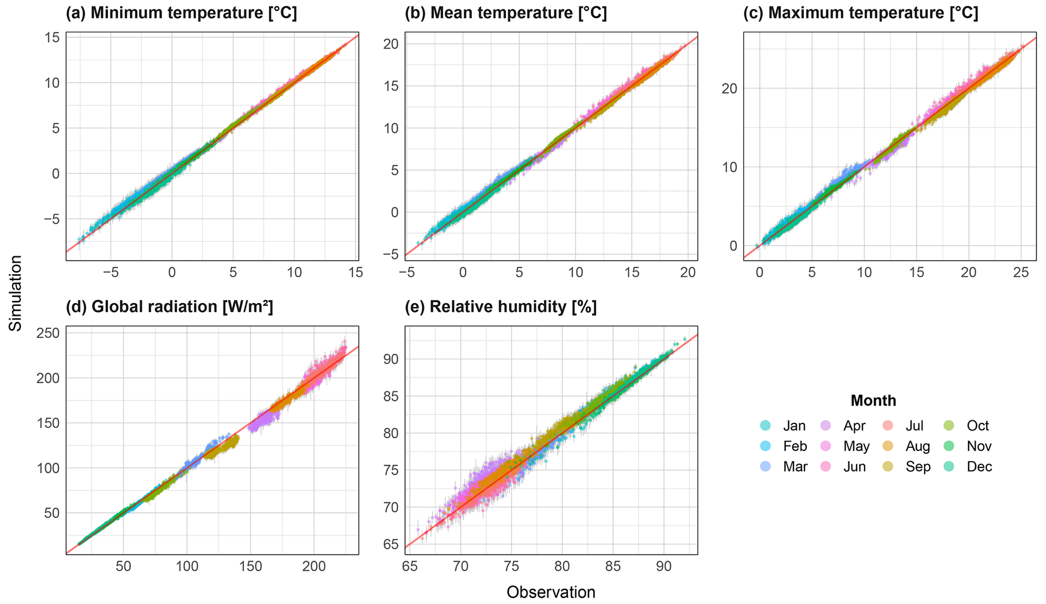
Figure 11 Scatter plots of mean monthly values for all catchments (N=400) for the variables minimum temperature (a), mean temperature (b), maximum temperature (c), global radiation (d) and relative humidity (e). The range from all realisations is shown via grey bars, and the median is shown coloured by month.

The reproduction of extreme catchment rainfall has been assessed via the bias in areal rainfall depth for a return period of 20 years for varying storm durations as shown in Fig. 10. For the 1 hour storm duration, winter performs significantly worse than for summer, especially regarding the median and range. This matches the result seen at the station level. The median annual result is close to zero, but with a wide overall range (±30 %). From a duration of 3 h and above, winter performs similarly to summer. A general underestimation (∼ 10 %) of extreme rainfall can be observed.

5.3 Non-rainfall climate variables

The non-rainfall climate variables were first assessed at the daily timestep (before disaggregation to hourly), to isolate errors arising from the k-NN resampling procedure.

Mean monthly values of all resampled climate variables are shown in the form of observed vs. simulated scatter plots (Fig. 11). All three temperature variables show a good reproduction over the year, with no systematic under or overestimation. Global radiation performs worse in both spring and summer, with the highest values showing greatest spread. The relative absolute bias is rarely greater than 5 % however. Relative humidity shows the greatest spread of values, particularly for the months April–July. For all variables, large variations across realisations were not shown.

The ability of the k-NN resampling procedure to maintain observed variable auto-correlation is shown in Fig. 12. The magnitude of auto-correlation is well preserved for all variables and all lags. As expected, a certain loss in auto-correlation is seen, particularly for lag 1. In general, it can be said that the temperature variables are the better performing ones. The auto-correlation results are sensitive to the weights used in the distance metric (Eq. 18). As these are user assigned, the performance relating to auto-correlation can be manipulated to a degree. The results here also show only small variations across realisations for all variables.

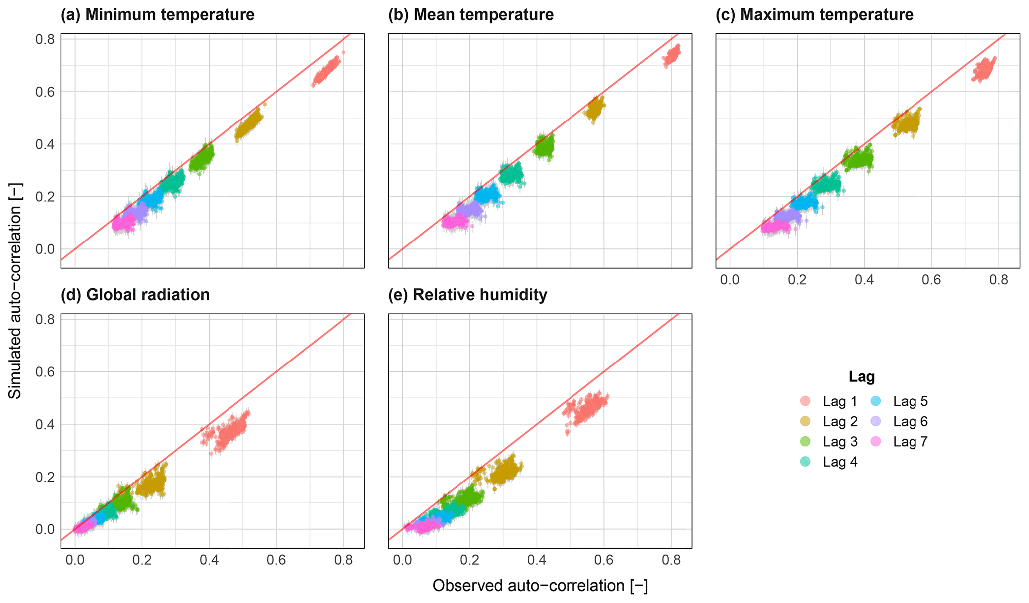
Figure 12 Scatter plots of variable auto-correlation for lags 1 to 7 for all catchments (N=400) for the variables minimum temperature (a), mean temperature (b), maximum temperature (c), global radiation (d) and relative humidity (e). The range from all realisations is shown via grey bars, and the median is shown coloured by month.

The Pearson correlation between resampled climate variables and daily rainfall is shown in Fig. 13. Also, here cross-correlation is reproduced well, however a loss in correlation is observed for all variables across most months. The temperature variables are worst performing during the winter months, where correlation is highest. Summer months, where a smaller negative correlation is observed, on average perform better, though with a greater spread of results. Relative humidity also performs worse for summer months. Correlation to global radiation is seen to be less dependent on month, and a general loss of correlation is observed.

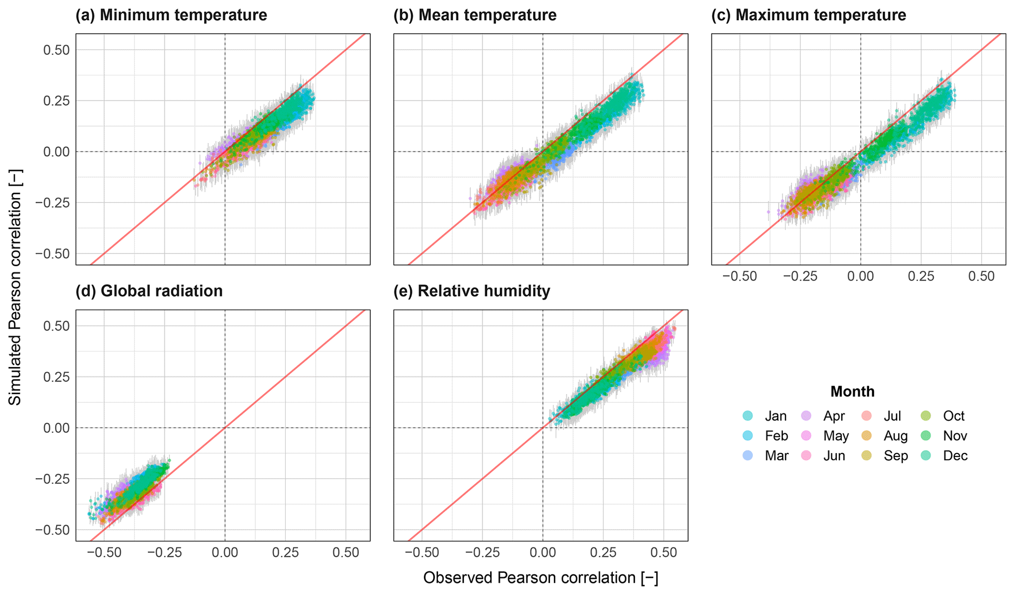
Figure 13 Scatter plots of correlation to daily rainfall for all catchments (N=400) for the variables minimum temperature (a), mean temperature (b), maximum temperature (c), global radiation (d) and relative humidity (e). The range from all realisations is shown via grey bars, and the median is shown coloured by month.

To assess errors stemming from the use of the gridded climate dataset, observed daily time series from 39 reference stations from the German Weather service where compared against corresponding HYRAS gridded values both before and after resampling (Fig. 14). Looking at the results before resampling (top row of Fig. 14), performance is generally good with absolute bias generally not exceeding 2 ^∘C for temperature. Radiation shows a very good reproduction of observations, whereas relative humidity in part shows a very poor reproduction. The results after resampling (bottom row of Fig. 14) mimic those of before, however with a small increase in bias, with temperature still performing very well, followed by global radiation and humidity. This shows that the use of the gridded dataset does not bring about a significant loss of performance, with the exception of relative humidity.

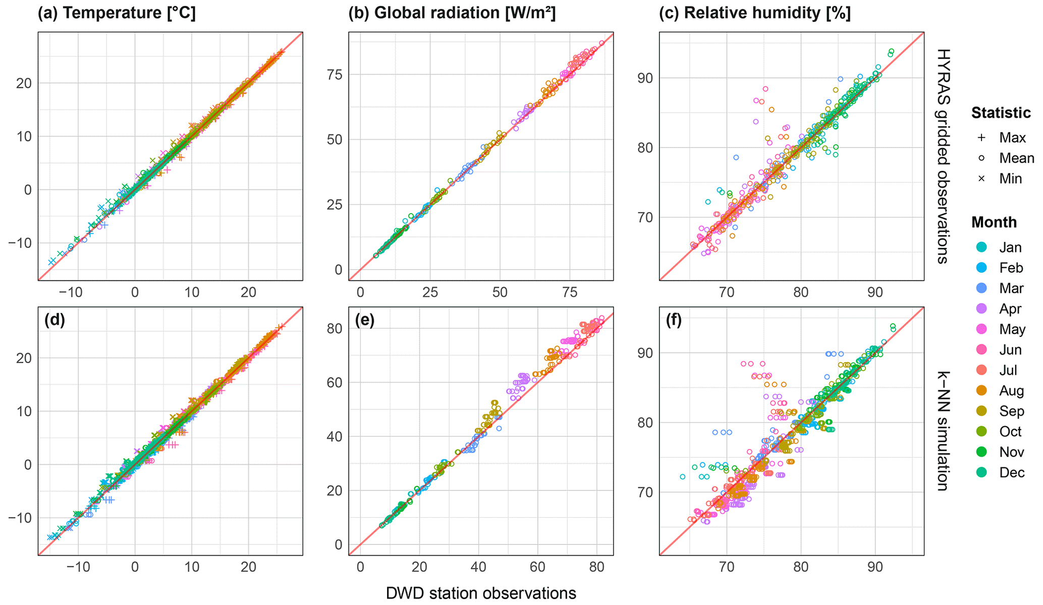
Figure 14 Scatter plots showing bias of mean monthly values of temperature (a), global radiation (b) and relative humidity (c) between point weather station observations and, (a, b, c) HYRAS gridded observations for the same time period (1976–2015), and (d, e, f) median bias from 37 × 40 year simulations after k-NN resampling. For temperature, values are further split by daily minimum, mean and maximum. As weather stations can overlap multiple catchments, more data points are included in the bottom plots. Temperatures were corrected for elevation difference between the grid cell elevation and weather station elevation using a lapse rate of 6.5 ^∘C km⁻¹.

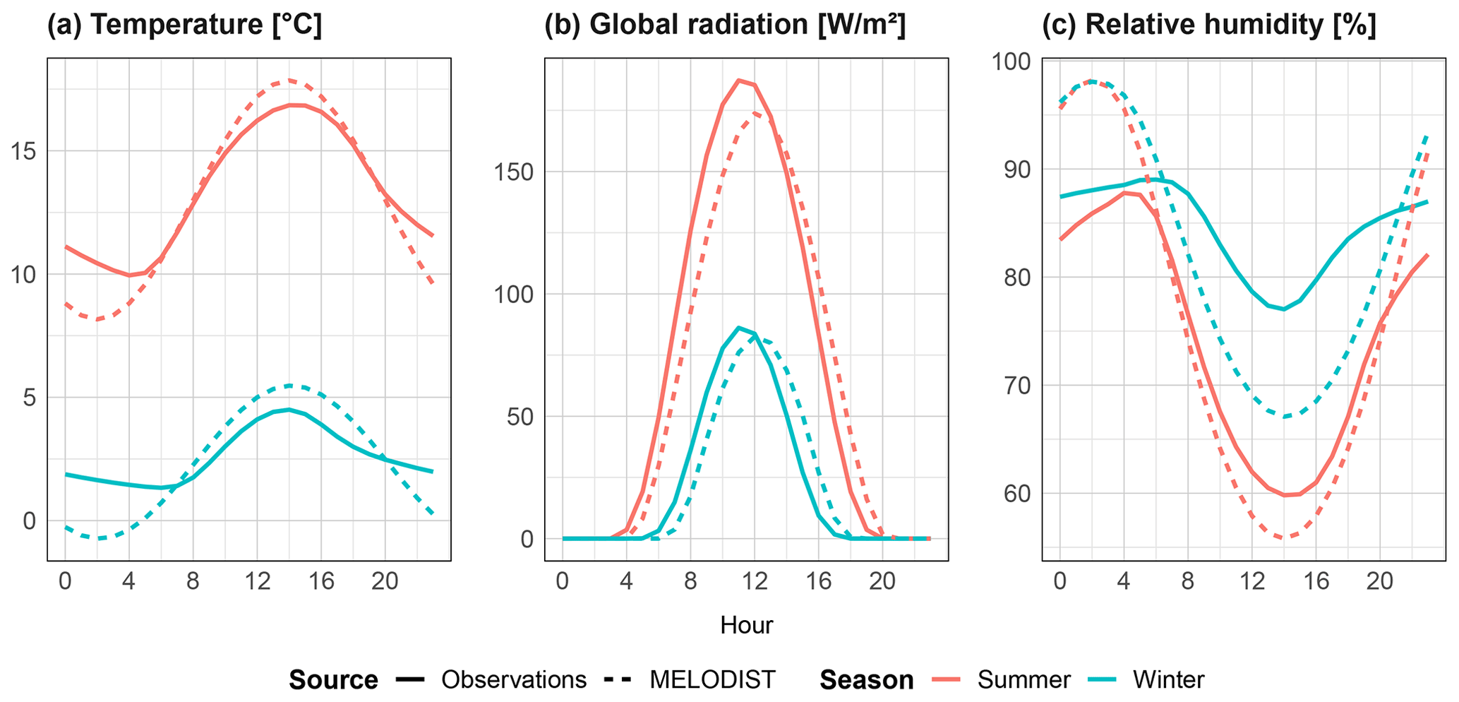
Figure 15 Mean hourly values of the non-rainfall climate variables temperature (a), global radiation (b) and relative humidity (c), separated by season for 39 DWD reference stations. Simulations show output from the MELODIST disaggregation model, using daily observations as input.

Finally the disaggregation to hourly performance is assessed by comparing hourly observed vs. simulated means of each climate variable, as shown in Fig. 15. Significant deviations between observed and simulated values can be seen, particularly for daily minimum values, and for relative humidity in winter. However, as the model's intended end-use is derived flood frequency analyses, the recreation of diurnal profiles is of lower priority. In contrast to the results from the k-NN resampling, global radiation is the best performing of the three resampled variables.

6 Conclusions

This study presents a major revision of the previous space–time rainfall model by Haberlandt et al. (2008). Large station networks of over 80 stations can now be modelled with limited loss in the observed spatial dependence structure. This was achieved by introducing a novel non-sequential branched event resampling approach based on a simulated annealing discrete optimisation procedure, extending the single-site rainfall model into space. While the current version does not consider advection or anisotropic properties, the optimisation procedure is flexible enough that such features could be incorporated in future model revisions by expansion of the objective function. Further modifications to the single-site rainfall model also resulted in improved model parsimony and performance regarding rainfall extremes.

Furthermore, the coupling of the space–time rainfall model to a non-parametric k-NN weather generator and subsequent disaggregation to hourly now provides the user a single tool for the generation of hourly climate time series for applications such as derived flood frequency analyses. Coupling the two sub-models via rainfall state allowed an adequate reproduction of both auto-correlations and correlation to rainfall. The flexibility of the approach allows the modelling of a diverse range of climate variables and observation sources (point or gridded).

By testing the complete model on 400 catchments and 699 rainfall stations across Germany, the model was shown to perform across a wide range of catchment sizes and location. Future studies may assess the performance in different climates and over more diverse terrain.

Currently, the space–time rainfall model is run separately for summer and winter seasons. This coarse partitioning is one potential area for future improvement. Conditioning the model on circulation patterns, which better categorise different rainfall and weather pattern types, may lead to increased performance, particularly regarding extremes. It may, however, be that a conditioning of the model on circulation patterns is too restrictive, especially as observation lengths of sub-daily rainfall are generally too short.