Direct integration of reservoirs' operations in a hydrological model for streamflow estimation: coupling a CLSTM model with MOHID-Land

Knowledge about streamflow regimes and values is essential for different activities and situations in which justified decisions must be made. However, streamflow behavior is commonly assumed to be non-linear, being controlled by various mechanisms that act on different temporal and spatial scales, making its estimation challenging. An example is the construction and operation of infrastructures such as dams and reservoirs in rivers. The challenges faced by modelers to correctly describe the impact of dams on hydrological systems are considerable. In this study, an already implemented solution of the MOHID-Land (where MOHID stands for HYDrodinamic MOdel, or MOdelo HIDrodinâmico in Portuguese) model for a natural flow regime in the Ulla River basin was considered as a baseline. The watershed referred to includes three reservoirs. Outflow values were estimated considering a basic operation rule for two of them (run-of-the-river dams) and considering a data-driven model of a convolutional long short-term memory (CLSTM) type for the other (high-capacity dam). The outflow values obtained with the CLSTM model were imposed in the hydrological model, while the hydrological model fed the CLSTM model with the level and the inflow of the reservoir. This coupled system was evaluated daily using two hydrometric stations located downstream of the reservoirs, resulting in an improved performance compared with the baseline application. The analysis of the modeled values with and without reservoirs further demonstrated that considering dams' operations in the hydrological model resulted in an increase in the streamflow during the dry season and a decrease during the wet season but with no differences in the average streamflow. The coupled system is thus a promising solution for improving streamflow estimates in modified catchments.

1 Introduction

Knowledge about streamflow, including water quantity and quality, is fundamental for monitoring and controlling the environmental impacts of several activities and situations, including infrastructure design, support in decision-making processes, irrigation scheduling, design and implementation of water management systems, environmental management, studies of river and watershed behavior, flood-warning control, optimal water resource allocation, prediction of droughts, and management of reservoir operations (Mehdizadeh et al., 2019; Mohammadi et al., 2021; Hu et al., 2021). However, the task of delivering information about streamflow can be challenging since it commonly assumes a non-linear behavior, being controlled by various mechanisms that act on different temporal and spatial scales (Wang et al., 2006). These non-linear forcings include meteorological conditions, land use, infiltration, morphological features of the river, and catchment characteristics (Mohammadi et al., 2021). The complex and laborious process of streamflow estimation is usually exacerbated when the natural regime flow is modified by anthropogenic activities and human decisions. In this sense, reservoirs are a major concern in hydrological modeling since most models are not prepared to directly consider the existence of such infrastructures and the resulting alterations caused to the natural regime flow by their operations (Dang et al., 2020). If hydrological models are prepared to study and comprehend the behavior of natural systems, the lack of information about reservoirs' operations, such as operating rules and flood contingency plans, poses a challenge for a correct representation of those infrastructures.

As pointed out by Dang et al. (2020), a post-process methodology is often used to impose reservoirs' operations on hydrologic–hydraulic models. This way, the need for modifying models' structures is avoided. However, Bellin et al. (2016) considered the direct representation of reservoir water storage and operation to be the best approach to correctly simulate such systems. Nevertheless, the challenges faced are many and have limited the number of studies carried out (Dang et al., 2020).

Recently, Xiong et al. (2019) developed a statistical framework where an indicator combining the effects of reservoir storage capacity and the volume of the multi-day antecedent rainfall input was used to assess the impact of a reservoir system on flood frequency and magnitude in downstream areas of the Han River, China. Yun et al. (2020) modified the structure of the variable infiltration capacity (VIC) model to include a reservoir module for estimating the variation of streamflow and flood characteristics when impacted by climate change and reservoir operation in the Lancang–Mekong River basin in southeast Asia. Also using a modified VIC model, Dang et al. (2020) simulated storage dynamics of water reservoirs again in the Lancang–Mekong River basin. In both studies, a comparison between the model results with and without reservoirs was provided. It is important to note that both Yun et al. (2020) and Dang et al. (2020) imposed operation rules on the model, with the former authors giving more importance to flood control and environmental protection and the latter focusing on energy production. Also, Hughes et al. (2021) used a modified version of the SHETRAN (Systeme Hydrologique Europeen TRANsport) model to simulate the streamflow considering the influence of reservoirs in Upper Cocker catchment, United Kingdom. The authors considered a weir model, and two tests were performed: (i) the weir was simulated as static (with closed sluice) to identify the sluice operating rules by means of a comparison of the results with the known outflow time series, and (ii) the weir model was run as non-static to implement the sluice operating rules deducted from the first approach. All studies mentioned above reproduced reservoirs' behaviors considering their operation rules, which, in most cases, are difficult to obtain or are very laborious to reproduce.

The application of operation rules may often be adapted to specific conditions, objectives, or constraints based on the knowledge and experience of operators (Yang et al., 2019). This makes the reservoirs' operations deviate from the reference operation curves, invalidating the sole use of physical-based models and the use of pre-established rule curves to reproduce the reservoir behavior in real time. To overcome this issue, Yang et al. (2019) indicated that machine learning methods, with their capacity to understand, extract, and reproduce complex high-dimensional relationships, can be an efficient and easy-to-use solution to reproduce reservoirs' operations, contemplating both the reference operation rules and the operators' historical experience. In this sense, the referred authors used recurrent neural network (RNN) models to extract reservoirs' operation rules from the historical operation data of three multipurpose reservoirs located in the upper Chao Phraya River basin, Thailand. Also considering the use of the geomorphology-based hydrological model (GBHM) to forecast the reservoir's inflow, Yang et al. (2019) achieved a real-time reservoir outflow forecast. Dong et al. (2023) proposed a similar approach to improve the reconstruction of daily streamflow time series in the upper Yangtze River basin, China. These authors proposed a practical framework to quantitatively assess the cumulative impacts of reservoirs' operations on the hydrologic regimes, coupling two data-driven models, namely an extreme gradient boosting (XGBoost) model and an artificial neural network (ANN) model with a high-resolution hydrologic model, and following a calibration-free conceptual reservoir operation scheme. The data-driven models were used to predict the outflow of reservoirs with historical operation data, while the calibration-free conceptual reservoir approach was used to simulate the outflow in data-limited reservoirs. The study presented by Dong et al. (2023) is a rare example of a promising solution for improving streamflow prediction in highly modified catchments, which this study aims to follow.

In the present study, the physical-based, distributed MOHID-Land model (Trancoso et al., 2009; Canuto et al., 2019; Oliveira et al., 2020) was coupled with a convolutional long short-term memory (CLSTM) model to estimate the daily outflow in Portodemouros reservoir, Galicia, Spain. The results obtained with the CLSTM model were estimated considering the reservoir's level and inflow simulated by MOHID-Land and were then imposed in that same model for streamflow simulation downstream of the reservoirs. However, the CLSTM model was first trained and tested using historical data. Thus, the main aim of this study is to verify the capacity of the coupled system to improve streamflow estimation downstream of Portodemouros reservoir. This study demonstrates the ability of the proposed approach to directly simulate reservoirs' operations in a hydrological simulation and validates a solution that is accessible and easy to implement.

2 Materials and methods

2.1 Description of the study area

The Ulla River watershed is located in the Galicia region, northwest of Spain, and drains an area of 2803 km², discharging into the Ría de Arousa estuary (Fig. 1). Ría de Arousa is one of the most important coastal water bodies in Galicia, having the Ulla and Umia rivers as major tributaries, and it is mainly used for recreative and fishery activities (da Silva et al., 2005; Outeiro et al., 2018; Blanco-Chao et al., 2020; Cloux et al., 2022). The maximum and minimum elevations of the Ulla watershed are 1160 and −1 m, respectively, and the main watercourse has a bed length of 142 km with its source at an altitude of 600 m. The watershed is inserted into an area characterized by a warm-summer Mediterranean climate (Csb) according to the Köppen–Geiger classification (Köppen, 1884). The annual precipitation is about 1100 mm, with rainy months from October to May. The annual average temperature is 12 ^∘C, reaching a maximum of 18 ^∘C in August and a minimum of 7 ^∘C in February. According to Nachtergaele et al. (2009), the main soil units in the Ulla river watershed are Umbric Leptosols and Umbric Regosols, representing 69 % and 31 %, respectively. The main land uses are forest, occupying 57 % of the area, and semi-natural and agricultural areas, covering 40 % (Copernicus Land Monitoring Service, 2016).

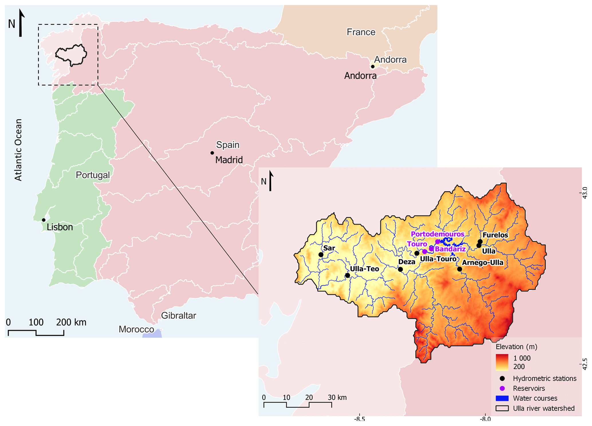
Figure 1 Ulla River watershed location, digital terrain model, and identification of hydrometric stations and reservoirs.

There are three reservoirs in the watershed: Portodemouros, Bandariz, and Touro (Fig. 1). Those reservoirs were constructed in cascade and work collectively, with Portodemouros placed at the beginning of the cascade, Touro at the end, and Bandariz in between. Portodemouros has a total capacity of 297 hm³, while Bandariz and Touro present much lower capacities, totalizing 2.7 and 3.8 hm³, respectively. Due to its significative storing capacity, Portodemouros reservoir can be used for flood control; however, the set of three reservoirs is mainly responsible for energy production. The patterns of daily inflow and outflow of the two last reservoirs are very similar since they are run-of-the-river dams (Fig. 2b and c). Nevertheless, Portodemouros works in a different way, presenting significative differences between the inflow and outflow patterns (Fig. 2a and d).

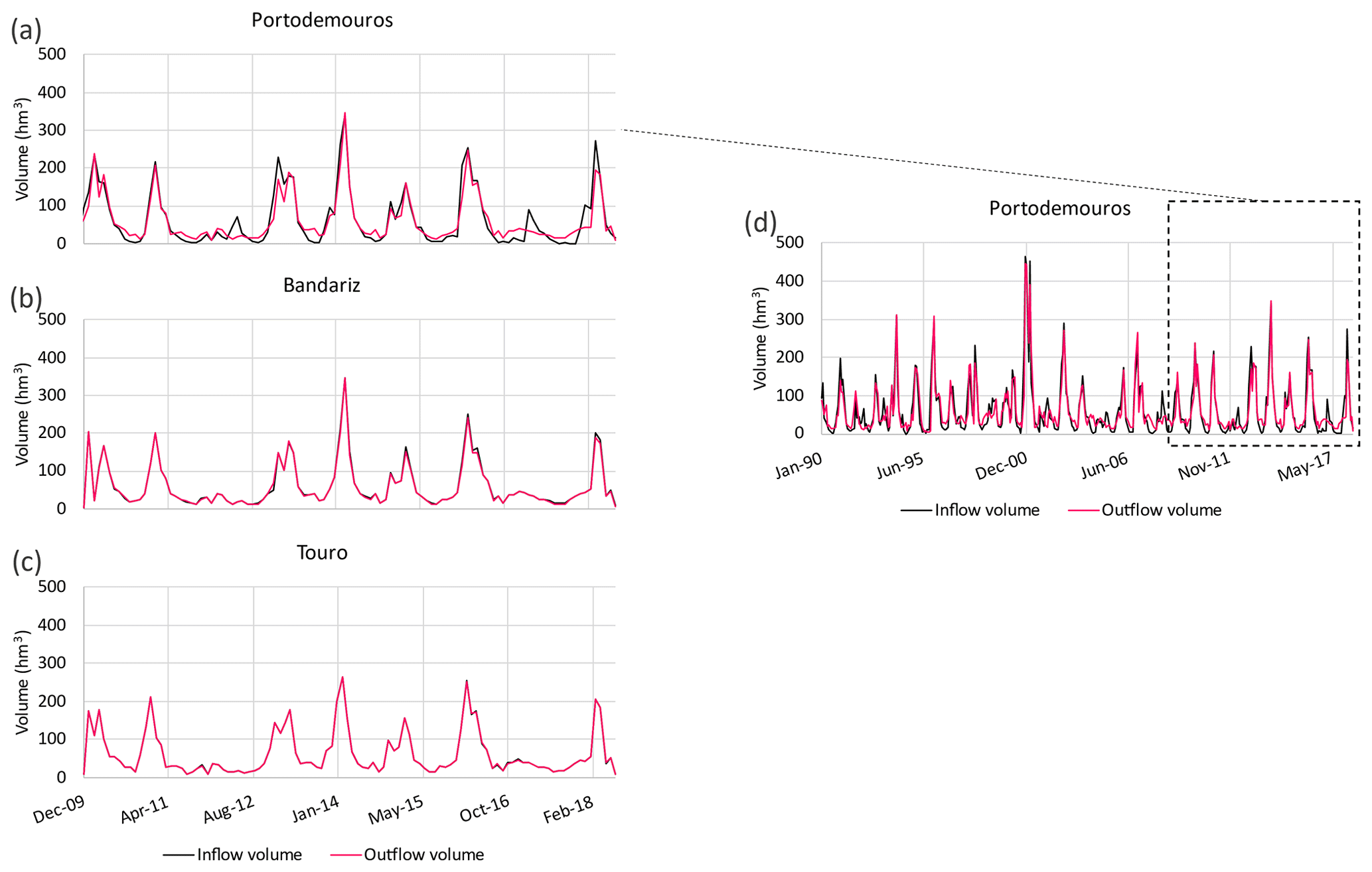
Figure 2 Comparison of inflow and outflow volumes in (a) Portodemouros, (b) Touro, and (c) Bandariz reservoirs for the period 2010–2018 and in (d) Portodemouros reservoir for the period 1990–2018.

2.2 MOHID-Land description

MOHID-Land is an open-source model (https://github.com/Mohid-Water-Modelling-System/Mohid, last access: 10 February 2019) and is part of the MOHID (hydrodynamic model) water modeling system. It is a fully distributed and physically based model adopting mass and momentum conservation equations considering a finite-volume approach (Trancoso et al. 2009; Canuto et al., 2019; Oliveira et al., 2020). The model estimates water fluxes between four main compartments, namely, the atmosphere; the soil surface; the river network; and the porous media, which is also intimately related to the vegetation compartment. Excepting the atmosphere compartment, which is only responsible for providing the meteorological data needed to impose surface boundary conditions, the processes in all the other compartments are explicitly simulated.

In MOHID-Land, the atmosphere compartment can deal with space- and/or time-variable data, and the input properties include precipitation, air temperature, relative humidity, wind velocity, and solar radiation and/or cloud cover.

The simulated domain is discretized considering two grids, one in the surface plane and the other in the vertical direction. While the first is defined according to the coordinate system chosen by the user, the last follows a Cartesian coordinate system. The surface water movement is computed considering a 2D surface grid and solving the Saint-Venant equation in its conservative form, accounting for advection, pressure, and friction forces. The Saint-Venant equation is also solved one-dimensionally (1D) for the river network. This network is derived from the digital terrain model represented in the 2D surface grid by connecting surface cell centers (nodes) and is characterized by a cross-section geometry defined by the user. The water fluxes between these two (2D and 1D) compartments are estimated according to a kinematic approach, neglecting bottom friction and using an implicit algorithm to avoid instabilities.

The porous media is discretized by combining the 2D surface grid with the vertical Cartesian grid, defining a 3D domain with variable thickness layers. This compartment can receive or lose water from the river network, with fluxes being computed considering a pressure gradient in the interface of these two mediums. Besides the water coming from the drainage network, the porous media also receives water from the infiltration process, which is calculated according to Darcy's law. In this 3D domain, the water movement is simulated using the Richards equation and considering the same grid for saturated and unsaturated flow. The soil hydraulic parameters are described using the van Genuchten–Mualem functional relationships (Mualem, 1976; van Genuchten, 1980). The saturation is reached when a cell exceeds the soil moisture threshold value defined by the user, and, in that case, the model considers the saturated conductivity to compute flow, with pressure becoming hydrostatic and corrected by friction. To compute the lateral flow, the horizontal saturated hydraulic conductivity is given by the product of the vertical saturated hydraulic conductivity (K_sat,ver) and a factor (f_h) set by the user.

The soil water loss is mainly due to the evapotranspiration process, which is computed taking into account weather, crop, and soil conditions. The reference evapotranspiration (ET_o) is first computed according to the FAO Penman–Monteith method (Allen et al., 1998). Then, the potential crop evapotranspiration (ET_c) is obtained by multiplying the ET_o by a single crop coefficient (K_c) representing standard crop conditions. ET_c values are then partitioned into potential soil evaporation and crop transpiration rates based on the leaf area index (LAI) following Ritchie (1972). LAI is simulated using a modified version of the EPIC model (Neitsch et al., 2011; Williams et al., 1989) and considering a heat units approach for crop development, the crop development stages, and crop stress (Ramos et al., 2017). The actual transpiration is calculated based on the macroscopic approach proposed by Feddes et al. (1978), where root water uptake reductions are estimated considering the presence of depth-varying stressors (Šimůnek and Hopmans, 2009; Skaggs et al., 2006). The actual soil evaporation is estimated from the potential soil evaporation by imposing a pressure head threshold value (ASCE, 1996).

To avoid instability problems and to save computational time, the model allows the use of a variable time step, which reaches higher values during dry seasons and lower values in rainy periods when water fluxes increase.

2.2.1 Reservoirs module

Besides the main modules described above, MOHID-Land can also consider the existence of reservoirs in the river network domain. The operation of a reservoir needs several characteristics to be defined, namely, the minimum and maximum volumes, the minimum outflow (the definition of the maximum outflow is optional), the curve defining the relation between the level and the stored volume, the type of operation, the location in terms of coordinates, and the identification of the node in the river network where the reservoir is placed. A reservoir's operation may be defined by the relationship between the level and the outflow as an absolute value or as a percentage of the inflow, the percentage of the stored volume and the outflow as an absolute value or as a percentage of the inflow, and the percentage of the stored volume and the outflow as a percentage of the maximum outflow. The user can also define the existence of discharges (in and/or out) and the state of the storage capacity (full, filled with a percentage of the total capacity, or empty) at the beginning of the simulation. In that sense, the reservoir module works with each reservoir as a box where a mass balance is performed. This mass balance takes into account the stored volume and the amount of water that enters and leaves the reservoir. The former considers the inflow from the river network and any input discharge defined by the user. The latter considers the outflow estimated by the type of operation and any output discharge defined by the user. The new stored volume is transformed into a level according to the level–volume curve specified by the user.

2.2.2 Model setup

The MOHID-Land model was already implemented, calibrated, and validated in the study area as detailed in Oliveira et al. (2020). This study was carried out from 1 January 2008 to 31 December 2017. Only the natural regime flow in the watershed was considered, with model calibration and validation using data from hydrometric stations not influenced by reservoirs' operations. A detailed description of the calibrated parameters resulting from the work done by Oliveira et al. (2020) is presented in Appendix A.

Reservoirs setup

The three reservoirs in the studied watershed were implemented according to the characteristics presented in Table 1. Their curves relating the level and the stored volume are given in Fig. 3. These data were made available by Augas de Galicia (Augas de Galicia, 2022), which is a public entity managing the Galicia Costa basin district.

Table 1 Implemented characteristics for Portodemouros, Bandariz, and Touro reservoirs.

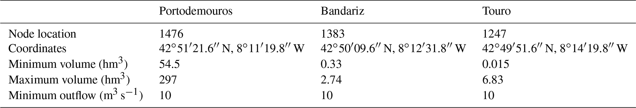
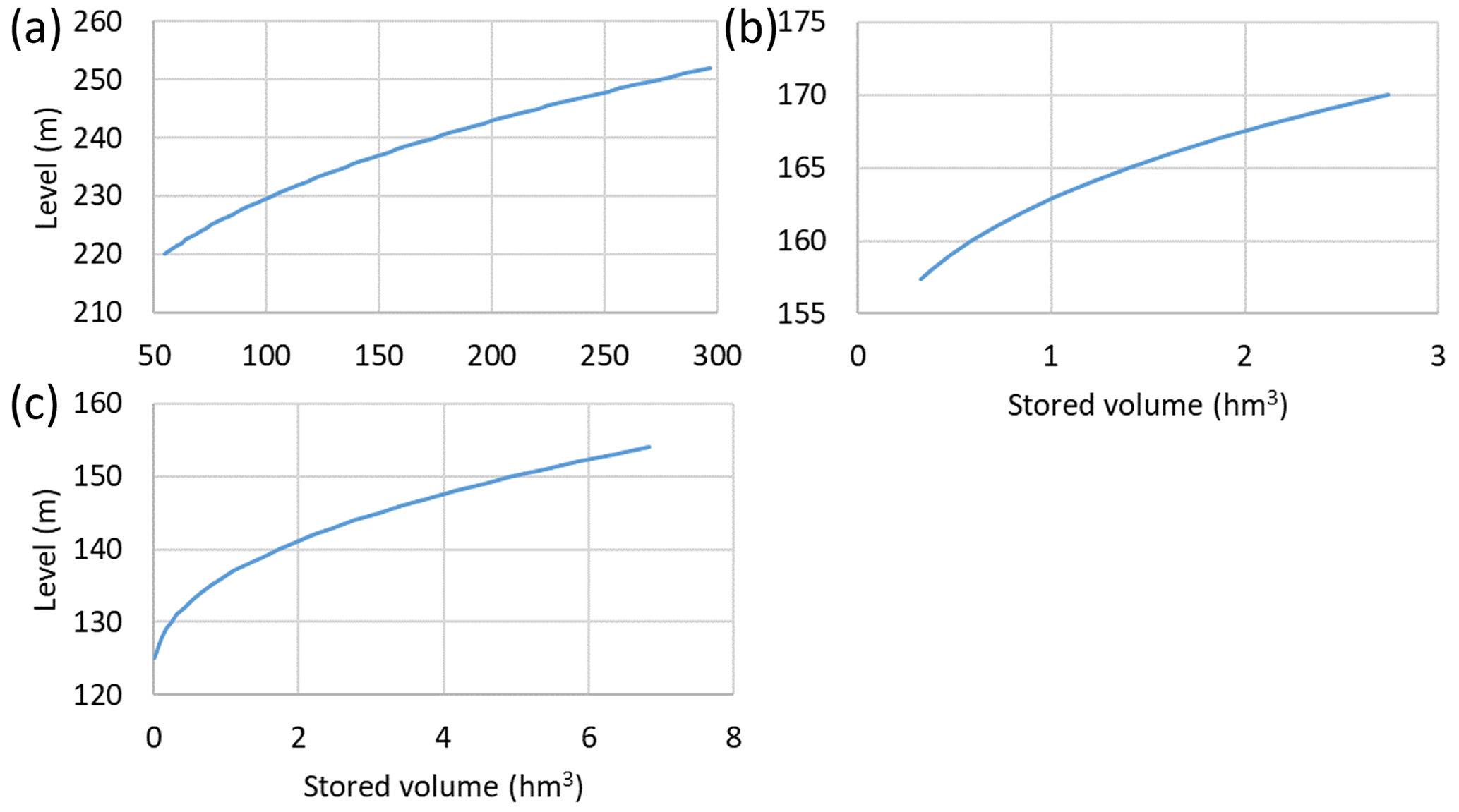
Figure 3 Level versus stored volume curves for (a) Portodemouros, (b) Bandariz, and (c) Touro reservoirs.

The operation for Bandariz and Touro reservoirs was defined based on the relation between the percentage of the stored volume and the outflow as a percentage of the inflow. If the stored volume was between 0 % and 95 %, the reservoir had no outflow. If the stored volume was above 96 %, the outflow equaled the inflow; i.e., the entire amount of water that entered the reservoir each instant left the reservoir in the same instant. For Portodemouros, no operation rule was set since there was no clear relation between the inflow and outflow values to be used in MOHID-Land. Thus, the daily outflow of Portodemouros reservoir was estimated using a neural network model and was imposed upon the hydrologic model as a time series. Additionally, if the stored volume of any reservoir was equal to or above the total capacity, the amount of water that reached the reservoir was transformed into outflow.

2.3 Neural network model for reservoir outflow estimation

To estimate Portodemouros reservoir's daily outflow, a neural network model was developed and tuned. It was composed of a combination of convolutional and long short-term memory layers, hereafter defined as the convolutional long short-term memory (CLSTM) model. This type of model was already applied for streamflow estimation by Ni et al. (2020) and Ghimire et al. (2021), who reported that, when compared with other neural network models, the CLSTM represented the best solution. The demonstrated good behavior of the CLSTM model is mainly related to its structure, which begins with the use of convolutional layers, responsible for the extraction of patterns in the input variables, and follows with long short-term layers, which are responsible for the prediction itself.

As referred to by Wang et al. (2019), convolutional neural networks (CNNs) have their origin in artificial neural networks (ANNs), but instead of fully connected layers, CNNs use local connections, giving more importance to high correlations with nearby data. Developed by LeCun and Bengio (1998) to identify handwritten digits, CNN uses convolutional filtering to achieve high correlation with neighboring data. This means that this type of network works based on the weight-sharing concept, with the filters' coefficients being shared for all input positions and their number and values being essential to capture data patterns (Wang et al., 2019; Barino et al., 2020; Chong et al., 2020). CNNs are thus recognized as more suitable solutions to identify local patterns, with a certain identified pattern being able to be recognized in another independent occurrence (Tao et al., 2019). As Ghimire et al. (2021) describe, CNN models can be used to identify patterns in one (1D), two (2D), or three (3D) dimensions. Being more adequate for time series data analysis, the 1D CNN solution was selected to be used in this study as an input layer. This selection avoided the manual feature extraction process since 1D convolutional algorithms are known for their powerful capability of doing this automatically. According to Huang et al. (2020), the time needed for training CNN models is one of its main weaknesses.

As a type of recurrent neural network (RNN) model, long short-term memory (LSTM) models are known for their capacity to maintain historical information about all the past events of a sequence using a recurrent hidden unit (Elman, 1990; LeCun et al., 2015; Lipton et al., 2015). This characteristic makes RNNs very suitable for time series data modeling (Bengio et al., 1994; Hochreiter and Schmidhuber, 1997; Saon and Picheny, 2017). However, RNN models demonstrate an inability in learning long-distance information because of their already known vanishing- and exploding-gradient problems during the training process (Ghimire et al., 2021). Trying to solve this RNN problem, Hochreiter and Schmidhuber (1997) developed the LSTM structure, which has the capacity to learn long-term dependencies (Xu et al., 2020).

2.3.1 Input data

The forcing variables were selected from a set that included the daily values of inflow, level, precipitation, temperature, and volume. The usage of the outflow values as a forcing variable was avoided because, when there are no observed values, the outflow data generated by the model must be used to feed the model itself, which can lead to an accumulation and propagation of errors in the estimated values. Several tests were performed considering different forcing variables and their combinations to verify which better estimate the daily outflow from the Portodemouros reservoir. Also, different time lags of those forcing variables were tested. The analysis of the test results shows that the best performance of the CLSTM model was obtained with inflow and level used as forcing variables, both considering the values from 1, 2, and 3 d before the forecasted day.

The daily values of inflow, level, and volume were provided by Augas de Galicia, and original hourly values of precipitation and temperature were obtained from the ERA5 Reanalysis dataset and were then accumulated or averaged considering a daily time step. The dataset made available by Augas de Galicia covered a period of about 29 years, with data from 1 January 1990 to 16 July 2018.

2.3.2 Structure

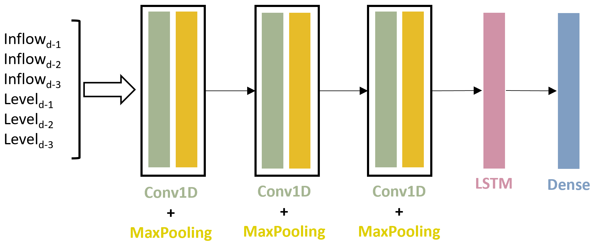
In this study, the model structure was developed using Python language and the Keras package (Chollet et al., 2015) on top of TensorFlow (Abadi et al., 2016). The types of layers made available by the Keras package and used here were the Conv1D, MaxPooling, LSTM, and dense. After several tests, the adopted model's structure included a Conv1D input layer followed by a MaxPooling layer. Then, two other sets of Conv1D plus MaxPooling layers were adopted. After those, an LSTM layer was introduced, and the output layer was selected to be a dense layer (Fig. 4).

Figure 4 CLSTM structure used in this study.

For the convolutional layers, no activation function was defined, while the LSTM layer was activated with the hyperbolic tangent function. For the output dense layer, the exponential linear unit function was used as activation function.

The optimizer, i.e., the training algorithm, was selected to be the Nadam algorithm, with a learning rate of 1 × 10⁻³ and an epsilon value of 1 × 10⁻⁷. The loss was estimated using the mean absolute error (MAE). Finally, the number of epochs and the batch size were, respectively, 300 and 20, found after a trial-and-error procedure.

2.3.3 Model optimization

The model optimization considered two phases, namely, the manual tuning of hyperparameters and the optimization of weights reached with the training process. In both cases, the structure presented above was exposed to a subset of the original dataset, i.e., the training dataset, where the forcing and target variables were included. The training dataset was handled and prepared with Pandas (McKinney, 2010) and scikit-learn (Pedregosa et al., 2011) packages, with the data being delayed with the first and scaled with the latter. The scaling function transformed the features of the given data into values within a desired range, which was defined from 0 to 0.9 considering that the maximum values of the variables cannot be represented in the dataset.

The tuning process was carried out to optimize the hyperparameters of the model. Several values for the number of filters, the kernel size for convolutional layers, and the number of units for the LSTM layer were tested. The best performance was reached with 16 filters and a kernel size of 10 for all three convolutional layers and 10 units for the LSTM layer. The pool size was set as 2 for the first and second MaxPooling layers and as 1 for the third layer of this type.

The training process consisted of changing the weights and bias values of a model to improve its capacity to estimate the target variable. The initialization of those values followed the default definitions of the Keras package for all the layers, which means that the weights were initialized according to the Glorot uniform method (Glorot and Bengio, 2010), and the biases were initialized with value 0. However, this type of initialization and the consequent training process have a random nature associated with them, repeatedly resulting in different estimations of the same target variable even when considering the same forcing variables and the same trained structure. To overcome this problem, the CLSTM model was exposed and trained and the final weights were saved 100 times, always considering the same training dataset, with the results being evaluated individually for each experiment. Based on these results, the model with the best performance was selected to estimate the outflow values for the Portodemouros reservoir.

2.4 Coupling MOHID-Land and CLSTM models

The operationality of the coupled system, which includes the CLSTM and MOHID-Land simulations, was divided into two phases, one that comprehended the warm-up period and the other including the calibration and validation periods defined in Oliveira et al. (2020). Since MOHID-Land is a physical model, it was necessary to consider an initial warm-up period for the stabilization of the hydrological processes and to avoid the influence of the errors related to the imposed initial conditions in the results.

In both phases, models were simulated on a daily basis, taking advantage of the possibility of doing continuous simulations in MOHID-Land. This means that, in every simulation, the state of the system in the last simulated instant is saved and can be used as the initial state in the next simulation if the date and time match.

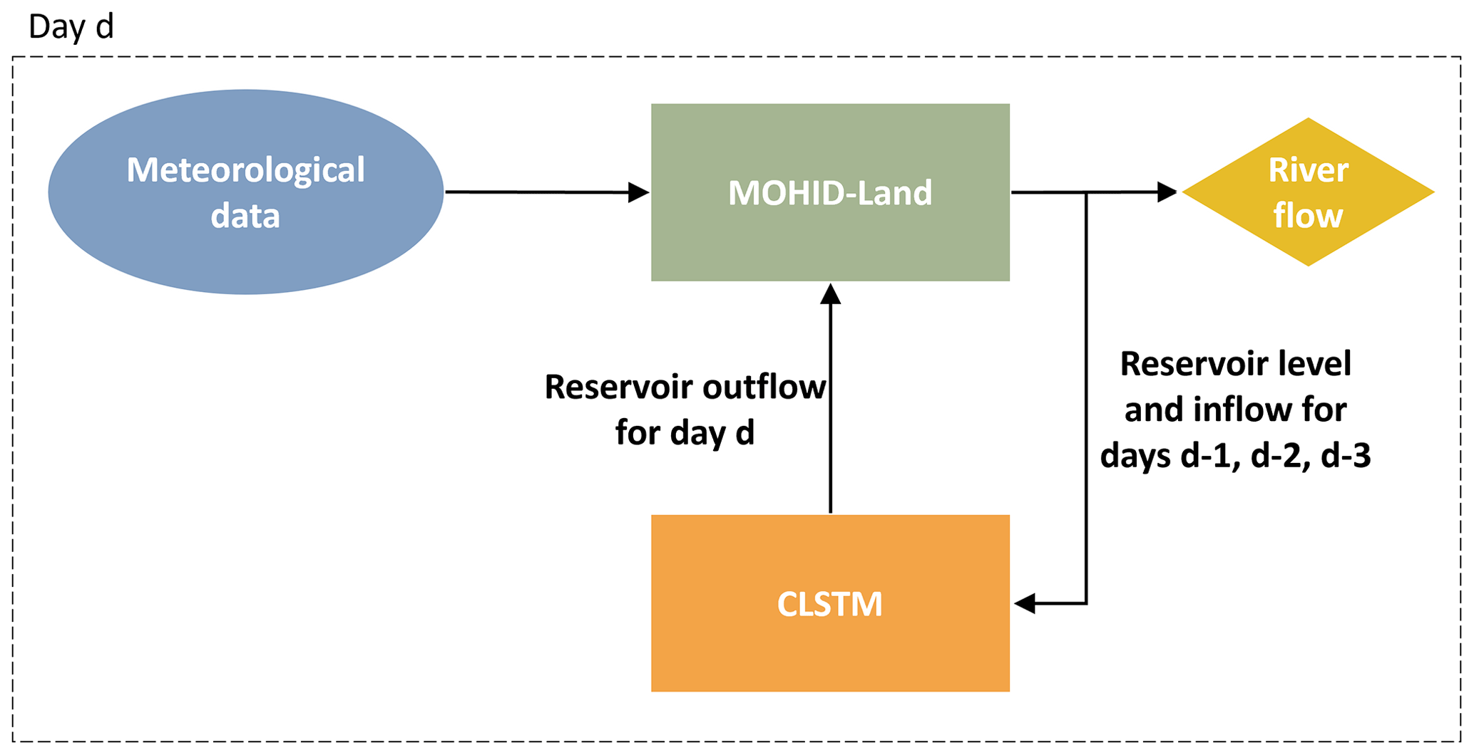
In the warm-up simulation, the reservoirs' module was deactivated. In the end of the warm-up period, the reservoirs' module was activated, and the initial conditions (level and stored volume) for the three reservoirs were manually imposed considering the measured values. Then, for each simulated day, the CLSTM model was the first to be run. The optimized model was loaded and received the information about the levels and the inflows of Portodemouros reservoir estimated by MOHID-Land for the 3 d before the simulated day. The CLSTM used this information to estimate the outflow for the simulated day. The outflow value estimated by the CLSTM model was then imposed in MOHID-Land. A scheme representing the described process to couple both models is presented in Fig. 5.

Figure 5 Operationality scheme for the modeling process.

2.5 Model's evaluation

The CLSTM model used to predict the outflow from Portodemouros reservoir was evaluated considering a subset of the original dataset from Augas de Galicia, which was not previously exposed to the trained model. That subset is known as a test dataset and contained pairs of forcing (inflow and level) and target (outflow) variables. Thus, the outflow was estimated based on the forcing variables and was then compared to the corresponding measured outflow. The test dataset corresponded to 10 % of the size of the original dataset and covered the period between 19 September 2015 and 16 July 2018, totalizing 1023 daily values.

In turn, the evaluation of streamflow values focused on the hydrometric stations placed downstream of the set of reservoirs and intended to verify the behavior of the coupled modeling system (MOHID-Land + CLSTM). This evaluation was performed by comparing the streamflow values estimated by the coupled modeling system with those measured in the Ulla–Touro and Ulla–Teo hydrometric stations. The validation of the coupled system was conducted from 1 January 2009 to 31 December 2017.

In both cases, the comparison between modeled and observed values was based on a visual inspection, and the estimation of four different statistical indicators, namely, the coefficient of determination (R²), the percentage bias (PBIAS), the ratio of the root mean square error to the standard deviation of observation (RSR), and the Nash–Sutcliffe modeling efficiency (NSE), which were computed using Eqs. (1)–(4), respectively:

$$\begin{array}{}\text{(1)}& {\displaystyle }{R}^{\mathrm{2}}={\left[{\displaystyle \frac{{\sum }_{i=\mathrm{1}}^p\left(X_i^{\mathrm{obs}}-X_{\mathrm{mean}}^{\mathrm{obs}}\right)\left(X_i^{\mathrm{sim}}-X_{\mathrm{mean}}^{\mathrm{sim}}\right)}{\sqrt{{\sum }_{i=\mathrm{1}}^p{\left(X_i^{\mathrm{obs}}-X_{\mathrm{mean}}^{\mathrm{obs}}\right)}^{\mathrm{2}}}\sqrt{{\sum }_{i=\mathrm{1}}^p{\left(X_i^{\mathrm{sim}}-X_{\mathrm{mean}}^{\mathrm{sim}}\right)}^{\mathrm{2}}}}}\right]}^{\mathrm{2}},\text{(2)}& {\displaystyle }\mathrm{PBIAS}={\displaystyle \frac{{\sum }_{i=\mathrm{1}}^p\left(X_i^{\mathrm{obs}}-X_i^{\mathrm{sim}}\right)}{{\sum }_{i=\mathrm{1}}^p{X}_i^{\mathrm{obs}}}}\times \mathrm{100},\text{(3)}& {\displaystyle }\mathrm{RSR}={\displaystyle \frac{\mathrm{RMSE}}{{\mathrm{SD}}_{\mathrm{obs}}}}={\displaystyle \frac{\sqrt{{\sum }_{i=\mathrm{1}}^p{\left(X_i^{\mathrm{obs}}-X_i^{\mathrm{sim}}\right)}^{\mathrm{2}}}}{\sqrt{{\sum }_{i=\mathrm{1}}^p{\left(X_i^{\mathrm{obs}}-X_{\mathrm{mean}}^{\mathrm{obs}}\right)}^{\mathrm{2}}}}},\text{(4)}& {\displaystyle }\mathrm{NSE}=\mathrm{1}-{\displaystyle \frac{{\sum }_{i=\mathrm{1}}^p{\left(X_i^{\mathrm{obs}}-X_i^{\mathrm{sim}}\right)}^{\mathrm{2}}}{{\sum }_{i=\mathrm{1}}^p{\left(X_i^{\mathrm{obs}}-X_{\mathrm{mean}}^{\mathrm{obs}}\right)}^{\mathrm{2}}}},\end{array}$$

where $x_i^{\mathrm{obs}}$ and $x_i^{\mathrm{sim}}$ are the outflow values observed and estimated, respectively, by the model on day i; $X_{\mathrm{mean}}^{\mathrm{obs}}$ and $X_{\mathrm{mean}}^{\mathrm{sim}}$ are the average outflow considering the observed and modeled values in the analyzed period; and p is the total number of days and/or values in this period.

According to Moriasi et al. (2015), the NSE must be higher than 0.50 for the model to be classified as satisfactory, higher than 0.70 to be good, and higher than 0.8 for a very good performance. The R² values should be higher than 0.60 for a satisfactory performance, higher than 0.75 for a good performance, and higher than 0.85 for a very good performance. Finally, PBIAS of ±5 % is a characteristic of a very good model, while a model with a PBIAS of ±10 % is classified as good. To be classified as satisfactory, a model's PBIAS should be ±15 %.

3 Results

3.1 MOHID-Land model

In a natural regime flow, MOHID-Land's performance reached satisfactory to good results at the Sar, Ulla, Arnego–Ulla, and Deza hydrometric stations (Table 2), as shown in Oliveira et al. (2020). The R² values ranged from 0.56 to 0.75 and 0.76 to 0.85 in the calibration (1 January 2009–31 December 2012) and validation (1 January 2013–31 December 2017) periods, respectively. The RSR showed values lower than 0.67 for all stations in both periods, while the NSE presented values from 0.55 to 0.72 in the calibration period and from 0.72 to 0.84 in the validation period. Finally, the PBIAS presented a slight overestimation of river flow at the Sar hydrometric station (calibration: 0.18 %; validation: 16.09 %), while at the other three stations, the model underestimated the river flow, with PBIAS values ranging from −12.29 % to −8.96 % and from −18.54 % to −4.35 % in the calibration and validation periods, respectively.

Table 2 Statistical indicators resulting from the comparison of the natural regime flow estimated by MOHID-Land with the observed streamflow values at six hydrometric stations (Cal. – calibration, Val. – validation; adapted from Oliveira et al., 2020).

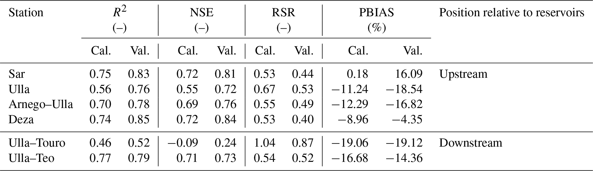
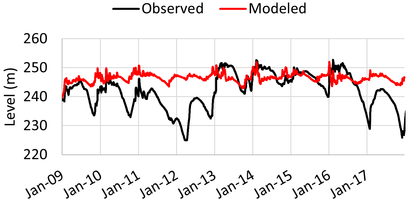
Figure 6 compares the observed streamflow (black line) with the respective MOHID-Land simulations without considering the influence of reservoirs (blue line) at Ulla–Touro and Ulla–Teo. Since these hydrometric stations have their natural regime flow altered by the operation of the set of reservoirs in the watershed, the performance of the hydrological model without reservoirs showed a significative decrease, as expected (Table 2).

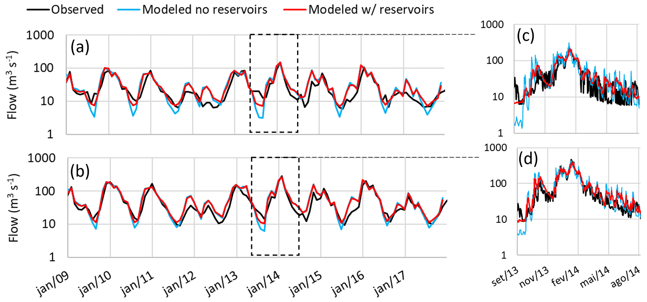
Figure 6 Comparison of modeled and observed average monthly streamflow in hydrometric stations (a) Ulla-Touro and (b) Ulla-Teo with and without considering the existence of reservoirs. Focus on the daily values for the period between September 2013 and September 2014 in (c) Ulla-Touro and (d) Ulla-Teo hydrometric stations.

3.2 CLSTM model

To better evaluate the performance of the CLSTM neural network model, the four statistical indicators were calculated for the set of 100 models trained with the same training dataset. Table 3 presents a summary of the results obtained.

Table 3 Average, minimum, maximum, and standard deviation values of the four statistical parameters estimated for the set of 100 models run and the elected model.

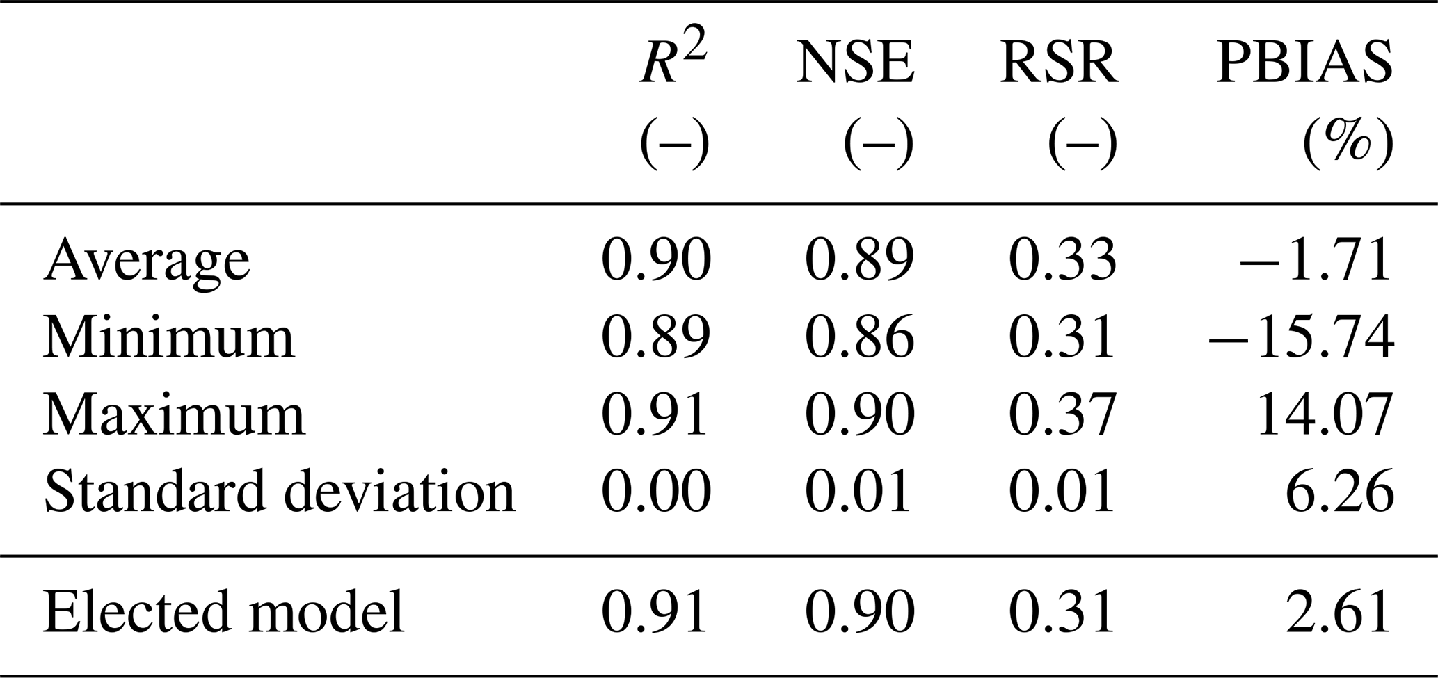
The behavior of the developed CLSTM model was extremely regular, with an R² above 0.89 and an NSE higher than 0.86. The worst PBIAS was −15.74 %, and the maximum value of RSR was 0.37. More specifically, the trained model elected to represent the outflow estimation of the Portodemouros reservoir obtained an NSE of 0.90, an R² of 0.91, a PBIAS of −2.61 %, and an RSR of 0.31. Figure 7 shows the comparison between the modeled and the observed values for Portodemouros outflow using observed levels and inflows to feed the model.

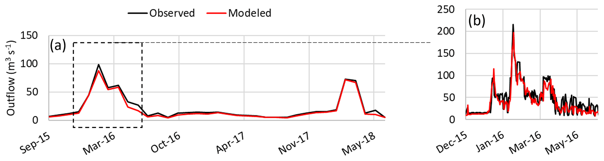
Figure 7 Comparison between modeled and observed Portodemouros outflow considering the CLSTM model: (a) monthly average and (b) daily values between December 2015 and June 2016.

The CLSTM predicted the outflow of the Portodemouros reservoir very accurately. However, when the observed values showed accentuated differences in a short period of time, such as 2 consecutive days, the model demonstrated some difficulty in reproducing that behavior, being able to reproduce the increase–decrease behavior at the right instant but being unable to reach the correct values. This is the case for the outflow predictions for May and June of 2016 (Fig. 7).

3.3 Coupled system

In the coupled system (MOHID-Land + CLSTM), the Portodemouros outflow was estimated with the CLSTM model considering the level and inflow estimated by the MOHID-Land model. Then, the outflow predicted by the CLSTM model was imposed upon MOHID-Land. Therefore, the inflow and outflow of the reservoir, as well as the two hydrometric stations influenced by the presence of the reservoirs, were the target of the validation of the coupled system.

Figure 8a compares the observed and modeled inflow in Portodemouros reservoir, while Fig. 8b shows the same comparison for the outflow. The observed (black line) and modeled (red line) streamflow comparisons for Ulla–Touro and Ulla–Teo stations are presented in Fig. 6a and b, respectively. The four statistical indicators used to evaluate the model's performance were also calculated for the inflow, outflow, and streamflow in Ulla–Touro and Ulla–Teo stations and are presented in Table 4.

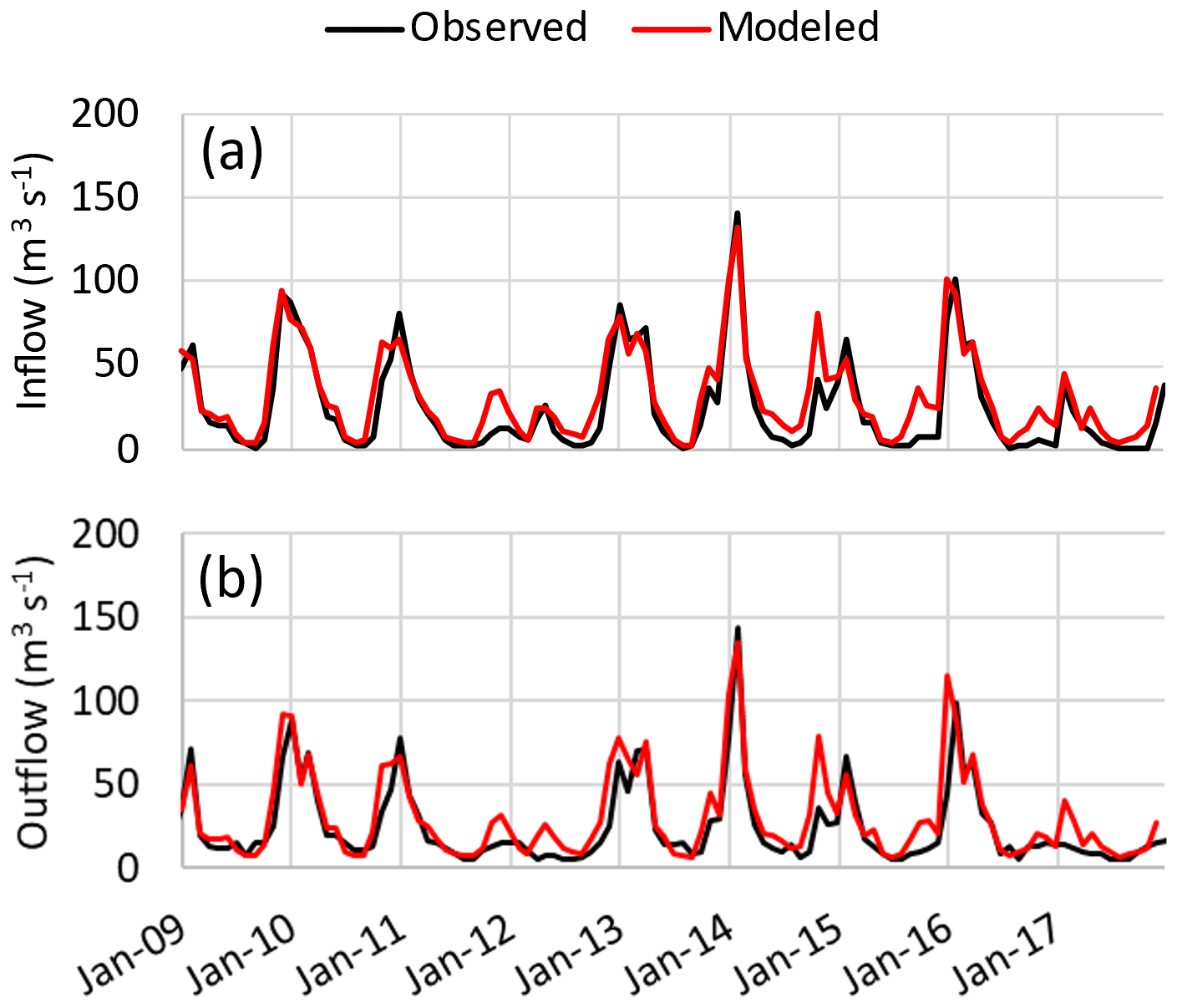
Figure 8 Comparison between the modeled and observed (a) inflow and (b) outflow in Portodemouros reservoir using the coupled system.

Table 4 Statistical parameters for inflow, outflow, and streamflow at Ulla–Touro and Ulla–Teo stations (Cal. – calibration, Val. – validation). The values between brackets represent the percentage change of the statistical parameter in relation to the corresponding value in the simulation without reservoirs.

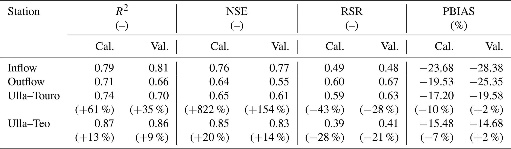
Inflows estimates in Portodemouros reservoir were in accordance with Oliveira et al. (2020). For the outflow values estimated with the CLSTM model considering the original dataset, the performance of the coupled system decreased slightly when compared with the previous indicators, with R² of 0.66, NSE of 0.55, RSR of 0.67, and PBIAS of −25 % for the validation period. The coupled system further showed a good performance when simulating streamflow at the two hydrometric stations (Ulla–Touro and Ulla–Teo), where the regime flow is altered by the presence of the reservoirs. Considering both hydrometric stations, the R² improved by about 30 % compared with the results without reservoir, reaching a minimum of 0.70. The RSR indicator also demonstrated a better performance with values fitting the range from 0.39 to 0.63 and revealing an average improvement of about 30 %. The higher impact was observed for the NSE indicator, which increased by about 253 %, with the values laying in the range from 0.61 to 0.85. Finally, the PBIAS showed an average decrease of about 4 %.

Despite the good results obtained for the streamflow of the downstream reservoirs, it is important to note that the reservoir's level estimated by MOHID-Land model did not reach the minimum requirements to be classified as satisfactory (calibration: NSE of 2.44, R² of 0.01, PBIAS of −3.16 %, RSR of 1.85; validation: NSE of 0.00, R² of 0.09, PBIAS of −0.67 %, RSR of 1.00). The coupled system overestimated the Portodemouros level most of the time, with an exception for the period between January 2013 and the middle of 2016, when the observed and modeled values were more similar (Fig. 9).

Figure 9 Comparison between modeled and observed level in Portodemouros reservoir.

It could be expected that this issue would affect streamflow estimation downstream of the reservoir since the outflow estimated by the CLSTM model considered the level values estimated by MOHID-Land. However, as demonstrated before, this issue did not significantly impact downstream results.

3.4 Impact of reservoir operation on streamflow

As referred to before, the reservoirs have an impact on the natural regime flow downstream of their infrastructures. The impact in the Ulla River watershed was here assessed by comparing the simulations under natural flow regime with the simulation of the coupled system. For this, the streamflow was evaluated in three locations along the river network, namely, at the Ulla–Touro and Ulla–Teo stations and at the outlet of the watershed. Table 5 shows the minimum; maximum; average; and second-, third-, and fourth-quartile values of the streamflow time series obtained for those locations considering the scenarios with (Res.) and without (No res.) reservoirs.

Table 5 Alterations to streamflow downstream of the reservoirs considering the simulations without and with those infrastructures (without reservoirs – No res.; with reservoirs – Res ).

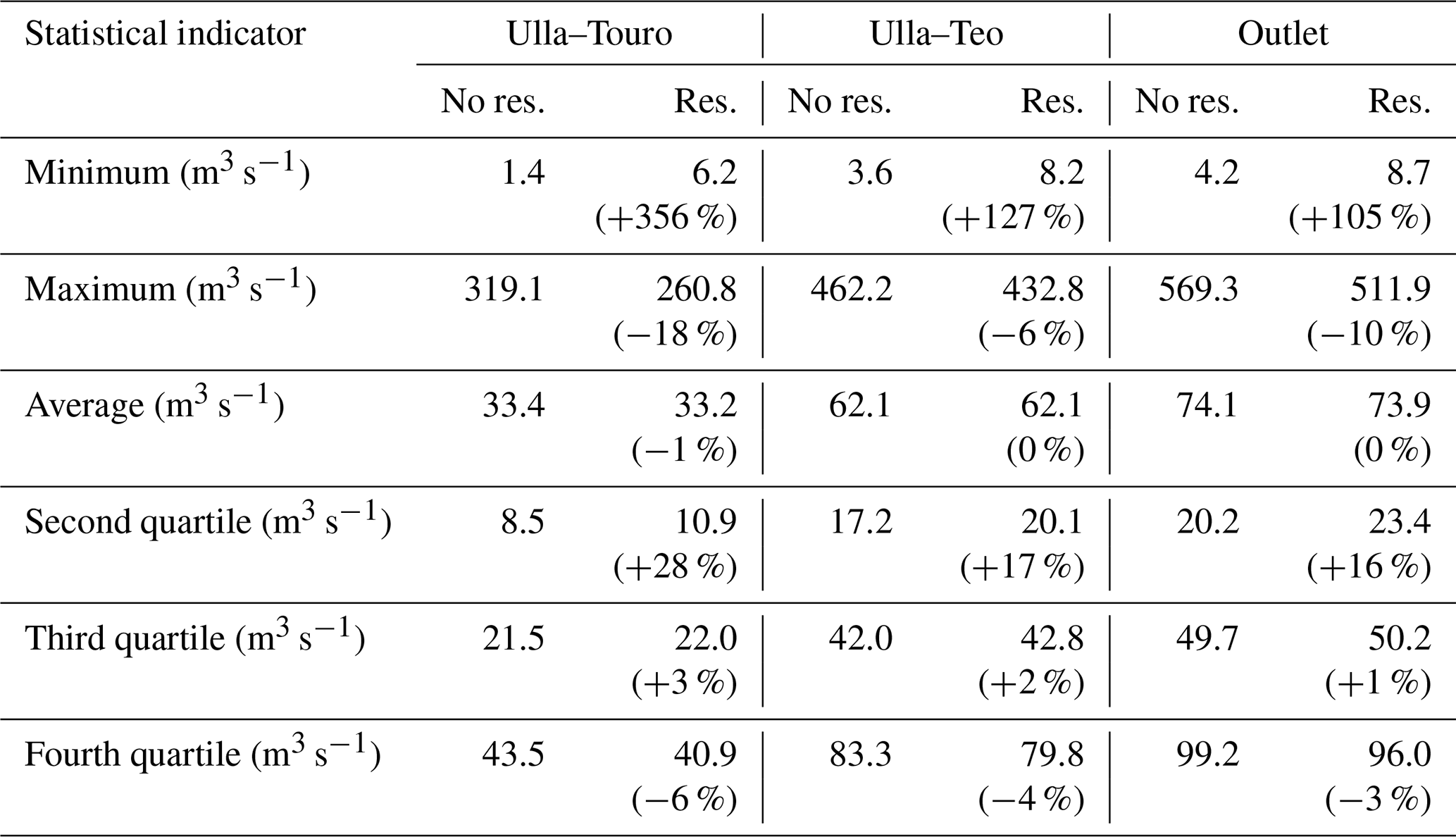
The most significative differences in streamflow occurred at the Ulla–Touro station, located immediately downstream of the reservoirs and more influenced by the reservoirs' operations. The main differences between the two scenarios were observed in the smallest values, namely, the minimum and the second-quartile values. In both cases, the streamflow showed an increase when the reservoirs were considered in the simulation, with the minimum streamflow increasing by 105 % in the outlet, by 127 % in Ulla–Teo, and by 356 % in Ulla–Touro and with the second quartile increasing by 16 %, 17 %, and 28 % in the outlet, Ulla–Teo, and Ulla–Touro, respectively. On the other hand, the main decreases were observed in the maximum and fourth-quartile values for all the evaluated points. However, the decreases of the highest values were not so significant compared to the differences observed for the smallest values, with the maximum values decreasing by 10 % in the outlet, by 6 % in Ulla–Teo, and by 18 % in Ulla–Touro and with the fourth quartile presenting differences of −3 %, −4 %, and −6 % in the outlet, Ulla–Teo, and Ulla–Touro, respectively.

The distribution of streamflow along the year (Fig. 10) showed a decrease in the average streamflow between October and December (wet season) when considering the reservoirs. Between January and March, also in the wet season, the streamflow only showed slight differences when considering or not considering the reservoirs. Finally, the dry season was totally characterized by an increase in the streamflow for the simulations with reservoirs, with the main differences being found between July and September. For the same reasons presented before, Ulla–Touro station was the point where the main differences were observed.

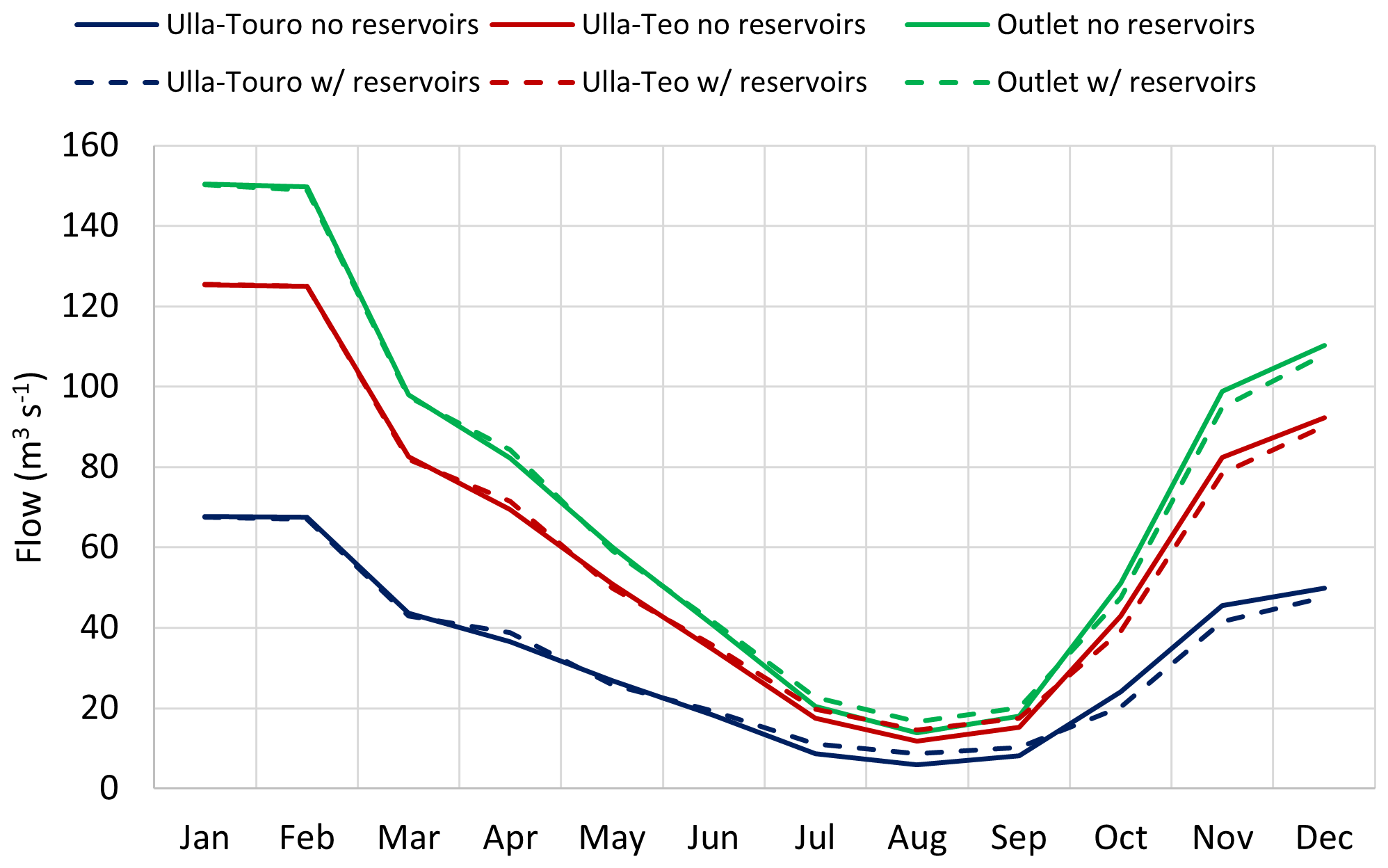
Figure 10 Average monthly streamflow in Ulla–Touro and Ulla–Teo stations and in the outlet for the two simulated scenarios, i.e., without and with reservoirs.

The behavior presented in Fig. 10 is the expected result when considering reservoirs' operations since this type of infrastructure is commonly used to store water during the wet season, causing a decrease of downstream streamflow. On the other hand, it is expected that average streamflow increases during dry seasons due to the constant necessity of energy production throughout the year and the imposition of ecological flows downstream of the reservoirs to maintain the health of the ecosystems.

4 Discussion

The results of the presented study show that the direct incorporation of reservoirs' operations in hydrologic modeling has a significative impact on the results of the modeled system, as already referred to by Bellin et al. (2016). The development of the CLSTM model for the prediction of Portodemouros outflow, which was afterwards imposed upon the hydrological model, needed to guarantee that the model estimation was good enough to avoid an error propagation. The elected CLSTM model reached a level of performance where the NSE was 0.90; the R² was 0.91; and the PBIAS and RSR were −2.61 % and 0.31, respectively, considering a test dataset. Similar results were obtained by Yang et al. (2019), who estimated the daily outflow of three multipurpose reservoirs located in Thailand considering three different types of RNN models, namely, a non-linear autoregressive model with exogenous input (NAXR), a long short-term memory (LSTM), and a genetic algorithm based on NAXR (GA-NAXR). The authors considered as forcing variables the inflow estimated by a hydrological model for the previous 2 d and the following 2 d together with the reservoir storage volume of the previous day. They obtained an average Pearson correlation coefficient of 0.91, an average NSE of 0.81, and an average PBIAS of −0.71 % with the NARX model and considering the three modeled reservoirs. The LSTM and GA-NARX models reached an average Pearson correlation coefficient of 0.88 and 0.94, respectively; an average NSE of 0.72 and 0.88; and an average PBIAS of 0.22 % and −0.24 %, with the GA-NARX demonstrating the best performance. Hughes et al. (2021) demonstrated the ability of a modified version of the SHETRAN model to predict the outflow of Crummock Water Lake, located in the Upper Cocker catchment in the United Kingdom. By including a dynamic weir module in the original SHETRAN model, the authors deduced the behavior of sluices by comparing the outflow values of static- and dynamic-weir models. The developed approach reached an NSE of 0.82, a value similar to the ones obtained in the present study, but its application to other case studies presents several limitations. First, it can be very laborious since it was based on a generic framework that included 12 steps. Second, the implementation of that framework implied a deep knowledge about the geometry of control structures and the details of operating procedures, with the authors referring to the fact that the broad conceptual understanding of sluice operations needed for the implementation was obtained through site visits and operator interviews.

On the other hand, the estimation of reservoirs' outflows using neural network models, such as the CLSTM model used here, can also present several limitations. As pointed out by several authors (ASCE, 1996; Maier et al., 2010; Dolling and Varas, 2002; Wu et al., 2014; Juan et al., 2017), the choice of the forcing variables is a crucial task for a successful model. Thus, the consideration of other possible forcing variables for the CLSTM model should be evaluated. Also, the structure of this type of model, which includes the number of hidden layers, the number of nodes, the kernel size, the activation functions, and other characteristics, is usually optimized by a trial-and-error procedure. However, the number of options that can be adopted for each of those structural characteristics and their combination makes the search space too wide to evaluate all the possible solutions. Thus, the manual approach adopted here to define the model's structure can be restrictive to the search for the best solution since a small number of possible solutions were tested when considering the entire search space. It is then clear that the optimization of the structure of the CLSTM model can improve the results. As suggested by Oliveira et al. (2023), this task can be done using tools that implement different algorithms to efficiently search for the best solution contained in a search space.

Considering the coupled system, the results showed a very clear and interesting improvement when compared with the implementation without reservoirs, with all the statistical indicators demonstrating a better performance in the coupled system for the two hydrometric stations influenced by reservoirs' operations. Although the coupled system has demonstrated a very good performance, it is important to refer to the fact that, besides the limitations already pointed out for the CLSTM model, the coupled system has its own limitations. Firstly, when CLSTM is incorporated into the system, it will use an estimated inflow, which is in opposition with the observed values used to train the model. Thus, when the inflow value is not correctly estimated by the hydrologic model, this will negatively influence the estimation of the outflow by the CLSTM model, leading to an exacerbation of the error downstream of this point. Also, the level used by the CLSTM model to force the outflow estimation is simulated by a mass balance performed by the hydrologic model. However, MOHID-Land does not yet incorporate the reservoir's loss by evaporation and infiltration, which can lead to an overestimation of the reservoir's level, as observed in Fig. 9. As in the case of the inflow, if the level value that feeds the CLSTM model is far from the correct value, the estimated outflow will also be inaccurate and may lead to an increased error in downstream areas. This is intimately related to the discussion presented by Kirchner (2006) about obtaining the right results for the right reasons, specifically where the author explores the limitations of the operational practice of hydrology. In that sense, the coupled system presented here, namely the CLSTM model, seems to be obtaining the right answer but for the wrong reasons. With the behavior of the CLSTM model being classified as a “black box”, without any physical constraints implemented, its results can be good enough while the model is exposed to conditions similar to those used for its optimization. However, when the forcing conditions go far beyond those used in the optimization, the results of these types of models become unreliable because of their lack of physical realism.

Nevertheless, the results of this study agree with those of other studies. For instance, Yun et al. (2020) modified the original VIC model to contemplate the reservoirs operations in the Lancang–Mekong River basin in Asia and compared the performance of the model with observed data from five hydrometric stations. Considering the calibration and validation periods, the authors obtained NSE values ranging from 0.61 to 0.75 and a model bias that varied between −3 % and 4 % for daily streamflow. Following a similar approach, Dang et al. (2020) modified the VIC model to integrate reservoirs' operations into hydrological simulations. A total of 118 solutions of the model with reservoirs and 109 solutions without reservoirs were run and automatically calibrated considering the upper Mekong River basin as a case study. That set of models obtained NSE values from 0.68 to 0.79 and a transformed root mean square error from 8.10 to 16.69, with the statistics of both solutions being evenly distributed in those ranges. It is important to note that the authors referred to the fact that, in the case of the implementations without reservoirs, the model probably reached such a good level of performance because the model parameterization helped to compensate for the structural error of the non-consideration of reservoirs. However, in both modified versions of the VIC model, reservoirs' operations were imposed by the authors through the definition of several operation rules that implied the knowledge of reservoirs' characteristics that sometimes are not easily available, such as the normal storage, the flood-limited storage, the environmental streamflow, the maximum safe streamflow for the downstream area, the capacity of the turbines, the target storage, and others. This fact can limit the application of both methodologies in areas with limited information.

Dong et al. (2023) adopted a similar approach to the one presented in this study, using two data-driven models to reproduce reservoir behavior in terms of outflow, when data was available, and coupling them with a high-resolution model. For the reservoirs with no data, a calibration-free conceptual reservoir operation scheme was designed. Considering the upper Yangtze River basin, China, as a case study, 10 reservoirs were considered, with 4 being simulated with the data-driven models and 6 being simulated with the conceptual scheme. The authors simulated the outflow and the storage of the reservoirs using a XGBoost model and an ANN model, with the first demonstrating the best performance for both properties. Considering the test period, XGBoost obtained NSE values higher than 0.85 for the outflow simulation and higher than 0.88 for the storage simulation, while the same indicator was higher than 0.80 and 0.83 for the outflow and storage simulations, respectively, when the ANN was considered. Taking into account the set of hydrometric stations analyzed, the NSE values were higher than 0.65.

Finally, the reservoir's downstream effects on the streamflow values found in this study were also in accordance with Yun et al. (2020) and Dong et al. (2023). Both studies concluded that the presence of the reservoirs decreased the average streamflow during the wet season and increased the average streamflow during the dry season, with a higher increase during the dry season than the decrease in the wet season. In the Ulla River basin, the annual average streamflow did not show any changes; however, the differences between wet and dry seasons were also observed (Fig. 10). During the wet season (October–March), the streamflow suffered a decrease of about 5 %, 3 %, and 2 % in Ulla–Touro, Ulla–Teo and the outlet of the watershed, respectively. For the dry season (April–September), increases of approximately 18 %, 9 %, and 8 % were estimated for those same points. At the same time, the maximum streamflow and the fourth-quartile values verified a decrease when the presence of the reservoirs was considered. The maximum streamflow decreased by a maximum of 18 % (from 319 to 261 m³ s⁻¹) at the Ulla–Touro station and by a minimum of 6 % (from 462 to 433 m³ s⁻¹), while the fourth quartile presented decreases between 6 % (from 44 to 41 m³ s⁻¹) and 3 % (from 99 to 96 m³ s⁻¹) at Ulla–Touro and at the outlet, respectively. The capacity of decreasing and controlling flow peaks is of extreme importance in the Ulla River basin since the downstream area is exposed to high flood risks, exacerbated by the combination of intense rainfall events and the influence of high tides (Augas de Galicia, 2019).

5 Conclusion

The approach presented and discussed in this work made possible the direct integration of reservoir operations into a hydrologic model. A CLSTM data-driven model was developed to estimate the reservoir outflows, the values of which were then imposed upon the MOHID-Land model. The case study focused on the Ulla River basin, which was the target of a previous work where MOHID-Land was implemented, calibrated, and validated for natural regime flow. In this watershed, a set of three reservoirs is present, with the reservoir more upstream having the higher storing capacity while the following two work as run-of-the-river dams. The operation of run-of-the-river dams was simulated with an operation curve that relates the level, the inflow, and the outflow of the reservoirs, and the outflow of the high-capacity reservoir was estimated using the CLSTM model. The target of this work was to analyze how streamflow simulations improved in the areas where the natural regime flow was modified by reservoirs' operations using the proposed coupled system. The main conclusions were as follows:

1. The CLSTM model selected to represent Portodemouros' outflow showed a very good performance, with NSE, R², and RSR values of 0.90, 0.91, and 0.31, respectively. The PBIAS was −2.61 %, indicating a very slight underestimation of the reservoir outflow.

2. The implementation of the coupled system demonstrated a significative improvement of streamflow estimations in areas downstream of the reservoirs, with the NSE increasing from a minimum of −0.09 without reservoirs to a minimum of 0.61 with reservoirs. Also, the R² demonstrated the same improvement, increasing from a minimum of 0.46 to 0.70 without and with reservoirs, respectively.

3. The MOHID-Land model failed to reproduce the level of the high-capacity reservoir, probably because the model does not include evaporation losses. However, the lack of accuracy did not have a significative impact on the performance of the coupled system in the calculation of daily streamflow.

4. According to the validation performed downstream of the reservoirs, the basic operation curves selected to simulate the function of the two run-of-the-river dams in the study domain seemed adequate.

5. For the modeled 10-year period, the impacts downstream of the reservoirs were in line with other studies, with the maximum streamflow (wet season) values experiencing a decrease and the minimum values (dry season) suffering an increase. However, the average streamflow did not show any increasing or decreasing tendency.

Besides the excellent results obtained in this study, future applications of the methodology should be tested and evaluated to understand its applicability to different scenarios. One of the doubts that remains is whether the CLSTM model has the capacity to reproduce the behavior of a reservoir where water is used for irrigation, which is characterized by punctual discharges in time, instead of an almost continuous discharge as in Portodemouros. Also, the capability of the trained CLSTM model in reproducing outflow values of other reservoirs with similar purposes should be addressed.

Appendix A

Following the sensitivity analysis performed, the best solution for the Ulla River model implementation was obtained considering a constant quadrangular horizontally spaced grid with 215 columns (west–east direction) and 115 rows (north–south direction) and a resolution of 0.005^∘ (∼ 500 m). The calibrated parameters were the K_sat,ver, the f_h factor, and the dimensions of the cross-sections in the river network.

The elevation of the calibrated solution was interpolated based on the digital terrain model from the European Environment Agency (European digital elevation model (EU-DEM), 2016), which has a resolution of 0.00028^∘ (∼30 m). The Manning coefficient for the river network was set to 0.035 s m${}^{-\mathrm{1}/\mathrm{3}}$, and the river cross-sections were assumed to be rectangular, with the dimensions varying according to the drained area of each node (Table A1 in the Appendix).

The surface Manning coefficients were specified based on the CLC 2012 (Copernicus Land Monitoring Service, 2016) data. For each land use, a Manning coefficient was first defined according to Pestana et al. (2013). Considering the interpolation process, those values varied from 0.023 to 0.298 s m${}^{-\mathrm{1}/\mathrm{3}}$. CLC 2012 data were further used to identify the vegetation in the watershed; these were made to correspond to data (vegetation growth parameters) in the MOHID's vegetation database. For each type of vegetation, a single crop coefficient (K_c) was adopted based on the tabulated values of Allen et al. (1998). After the interpolation process, the K_c values varied from 0.15 to 1.0.

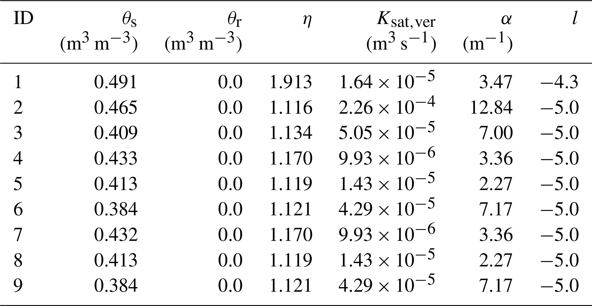
The soil domain was vertically discretized considering three horizons that comprehended six grid layers. The layers had variable thicknesses, increasing from the surface to the bottom: 0.3 (surface), 0.3, 0.7, 0.7, 1.5, and 1.5 m (bottom). The first horizon included the first two layers, while the second horizon included the two middle layers, and, finally, the bottom horizon considered the last two layers. The van Genuchten–Mualem soil hydraulic parameters were obtained from the multi-layered European Soil Hydraulic Database (ESHD, Tóth et al., 2017). For the surface horizon, ESHD data at 0.3 m depth were used to represent soil hydraulic data; ESHD data at 1.0 m depth were used to characterize the middle horizon; ESHD data at 2.0 m depth described the bottom horizon. In each of these horizons, three different sets of soil hydraulic data were identified (Fig. A1 in the Appendix). After the model's calibration, the van Genuchten–Mualem soil hydraulic parameters assumed the values presented in Table A2 for each set. The horizontal saturated hydraulic conductivity was obtained assuming an f_h equal to 10.

The meteorological boundary conditions were extracted from the ERA5 Reanalysis dataset (Hersbach et al., 2017), which is a gridded product with a resolution of 0.28125^∘ (∼31 km) and which makes available meteorological variables with an hourly time step. The variables used and interpolated to the case study grid were the u and v components of wind velocity at 10 m height, dew point and air temperatures at 2 m height, surface solar radiation downwards, surface pressure, total cloud cover, and total precipitation.

Table A1 Cross-section dimensions.

Figure A1 Soil IDs for each horizon: (a) surface, (b) middle, and (c) bottom horizons.

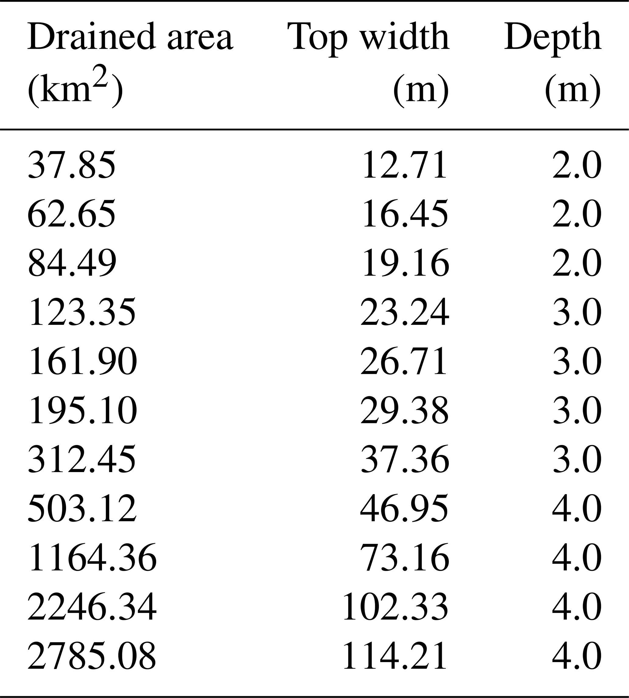
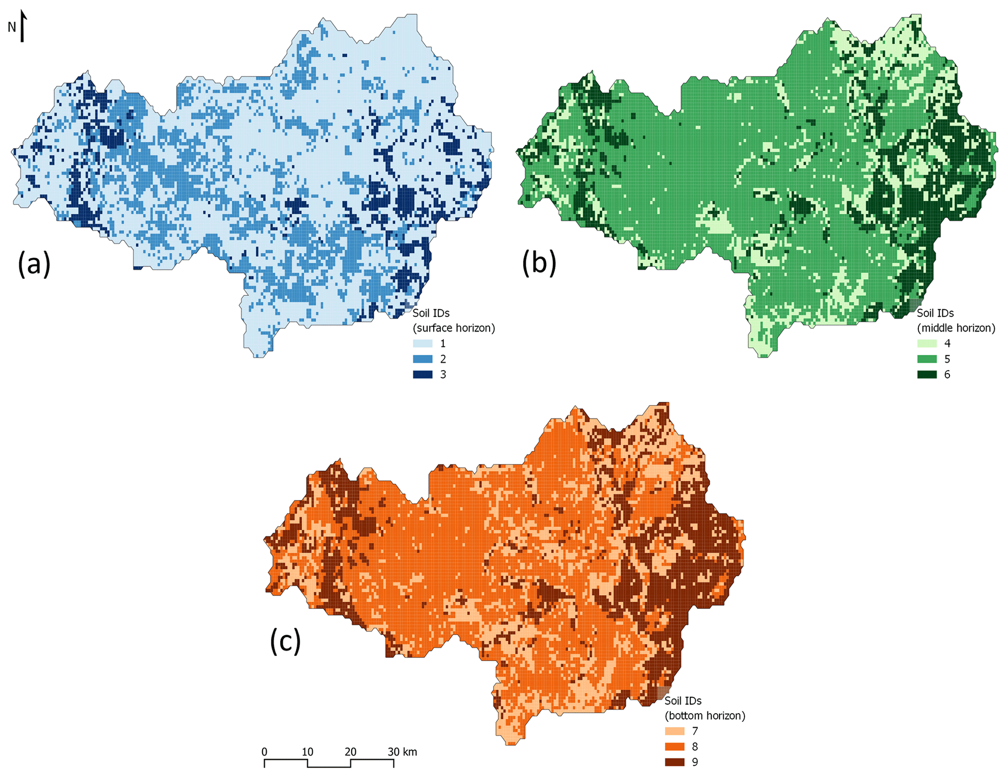
Table A2 Soil hydraulic properties by soil ID: θ_s – saturated water content, θ_r – residual water content, η and α – empirical shape parameters, K_sat,ver – vertical saturated hydraulic conductivity, and l – pore connectivity and/or tortuosity parameter.